Future Changes in Oceanography and Biogeochemistry Along the Canadian Pacific Continental Margin

Model projections of ocean circulation and biogeochemistry are used to investigate large scale climate changes under moderate mitigation (RCP 4.5) and high emissions (RCP 8.5) scenarios along the continental shelf of the Canadian Pacific Coast. To reduce computational cost, an approach for dynamical downscaling of climate projections was developed that uses atmospheric climatologies with augmented winds to simulate historical (1986–2005) and future (2046–2065) periods separately. The two simulations differ in initial and lateral open boundary conditions. For each simulation, the daily climatology of surface winds in the driving model was augmented with high-frequency variability from an atmospheric reanalysis product. The “time-slice” approach was able to reproduce the observed climate state for the historical period. Sensitivity tests confirmed that the high frequency wind variability plays an essential role in freshwater distribution in this region. Projections suggest that sea surface temperature will increase by 1.8–2.4°C and surface salinity will decrease between −0.08 and −0.23 depending on whether a moderate or high emissions scenario is used. Stratification increases throughout the region and there is some evidence of nutrient limitation near the surface. Primary production and phytoplankton productivity (chlorophyll) also increase. Density surfaces are relocated deeper in the water column and this change is mainly driven by surface heating and freshening. Changes in saturation state are mainly due to anthropogenic CO₂ with minor contributions from solubility, remineralization and advection. There is little difference between RCP 4.5 and RCP 8.5 with regard to projections of deoxygenation and acidification. The depths of the aragonite saturation state and the oxygen minimum zone are projected to become shallower by ≃ 100 and ≃ 75 m respectively. Extreme states of temperature, oxygen and acidification are projected to become more frequent and more extreme, with the frequency of occurrence of $\left[{\mathrm{\text{O}}}_2\right]<60\mathrm{\text{ mmol}}{\mathrm{\text{m}}}^{-3}$ expected to approximately double under either scenario.

1. Introduction

Increasing atmospheric greenhouse gas (GHG) concentrations affect marine ecosystems worldwide through a variety of mechanisms, notably ocean acidification due to dissolution of atmospheric CO₂ and declining oxygen concentrations (deoxygenation). Canadian Pacific coastal waters are often considered to be particularly vulnerable because waters rich in dissolved inorganic carbon (DIC) and low in oxygen are naturally present at relatively shallow depths on the continental slope (e.g., Feely et al., 2008). Warming of the surface ocean results in both declining surface oxygen concentrations, and increased stratification that leads to reduced ventilation of the subsurface ocean. Rising temperature, acidification, and declining oxygen are three important stressors that affect marine biodiversity and ecosystem health both individually and synergistically (Gruber, 2011; Pörtner et al., 2014). Climate change may also result in changes to the upwelling- and downwelling-favorable winds that play a major role in the oceanography of the Canadian Pacific continental margin (Merryfield et al., 2009; Foreman et al., 2014).

Episodes of extremely hypoxic or corrosive water have already led to extensive die offs of marine life in the region (Barton et al., 2015; Chan et al., 2019). To manage marine ecosystems under a changing climate and plan potential strategies for adaptation, projections of how physical, chemical, and biological characteristics of the ocean ecosystem will change are needed. Regional ocean downscaling of climate projections from global Earth System models are the only available source of information beyond the very limited time scales on which forecasting is possible (e.g., Li et al., 2019).

Estimates of projected changes in ocean state can be used, in combination with species observations, to estimate impacts on marine ecosystems. By identifying habitat changes, potential hot-spots and refugia, climate projections can be used to inform marine conservation and spatial planning. Additionally, projected ocean changes are a precursor to investigations of climate impacts on the goods and services that these ecosystems provide including, for example, the catch potential for various marine species (Cheung et al., 2010).

We present here a high-resolution regional projection of future climate for the Canadian Pacific continental margin. The point of departure for this work is Foreman et al. (2014) which examined changes in the physical oceanography of the British Columbia (BC) Continental Shelf. Our model includes biogeochemistry, has a higher resolution and uses an approach to dynamically downscaling climate projections that reduces computational costs. This work will evaluate the model's ability to reproduce the observed state of the ocean in the historical-climate simulation, present projections of the future ocean biogeochemical state, and evaluate the mechanisms underlying the projected changes.

2. Materials and Methods

This study uses a multi-stage downscaling approach to dynamically downscale global climate projections at a 1/36° (1.5 − 2.25 km) resolution. We chose to use the second-generation Canadian Earth System model (CanESM2) because high-resolution downscaled projections of the atmosphere over the region of interest are available from the Canadian Regional Climate Model version 4 (CanRCM4). We used anomalies from CanESM2 with a resolution of about 1° at the open boundaries, and the regional atmospheric model, CanRCM4 (Scinocca et al., 2016) for the surface boundary conditions. CanRCM4 is an atmosphere only model with a 0.22° resolution and was used to downscale climate projections from CanESM2 over North America and its adjacent oceans.

The model used is computationally expensive. This is due to the relatively high number of points in the domain (715 × 1,021 × 50) and the relatively complex biogeochemical model (19 tracers). Therefore, rather than carrying out interannual simulations for the historical and future periods, we implemented a new method that uses atmospheric climatologies with augmented winds to force the ocean. We show that augmenting the winds with hourly anomalies allows for a more realistic representation of the surface freshwater distribution than using the climatologies alone.

Section 2.1 describes the ocean model that is used to estimate the historical climate and project the ocean state under future climate scenarios. The time periods are somewhat arbitrary; 1986–2005 was chosen because the Coupled Model Intercomparison Project Phase 5 (CMIP5) historical simulations end in 2005 as no community-accepted estimates of emissions were available beyond that date (Taylor et al., 2009); 2046–2065 was chosen to be far enough in the future that changes in 20 year mean fields are unambiguously due to changing GHG forcing (as opposed to model internal variability) (e.g., Christian, 2014), but near enough to be considered relevant for management purposes.

While it is true that 30 years rather than 20 is the canonical value for averaging over natural variability, in practice the difference between a 20 and a 30 year mean is small (e.g., if we average successive periods of an unforced control run, the variance among 20 year means will be only slightly larger than for 30 year means). Also, there is concern that longer averaging periods are inappropriate in a non-stationary climate (Livezey et al., 2007; Arguez and Vose, 2011). We chose 20 year periods because they are adequate to give a mean annual cycle with little influence from natural variability, while minimizing aliasing of the secular trend into the means. As the midpoints of the two time periods are separated by 60 years, the contribution of natural variability to the differences between the historical and future simulations is negligible e.g., (Hawkins and Sutton, 2009; Frölicher et al., 2016).

Section 2.2 describes how climatologies derived from observations were used for the initialization and open boundary conditions for the historical simulations and pseudo-climatologies were used for the future scenarios. The limited availability of observations means that the years used for these climatologies differs somewhat from the historical and future periods. Section 2.3 details the atmospheric forcing fields and the method that we developed to generate winds with realistic high-frequency variability while preserving the daily climatological means from the CanRCM4 data. Section 2.4 shows the equilibration of key modeled variables to the forcing conditions.

2.1. Northeast Pacific Model Description and Forcing Fields

The regional model is based on the Nucleus for European Modeling of the Ocean (NEMO) numerical framework version 3.6 (Madec, 2008). The North–Eastern Pacific (NEP) model domain spans the Canadian Pacific Ocean east of ≃ 140°W and north of 45°N (Figure 1A). The horizontal resolution is nominally 1/36° latitude and longitude which gives a variable grid spacing between 1.5 and 2.25 km (Figure 1A).

FIGURE 1

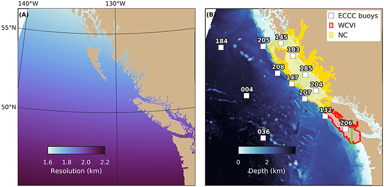
Figure 1. Maps of the (A) NEP36 model domain and resolution and (B) the model bathymetry. (B) Shows the focus regions of West Coast Vancouver Island (WCVI) and the Northern Coast (NC) as well as the positions of weather buoys maintained by Environment and Climate Change Canada. The green line shows the location where a vertical cross-section was extracted.

The model, referred to as NEP36, is an update of the model developed by Lu et al. (2017) based on NEMO version 3.1 and uses the same bathymetry (Figure 1B). The sea-ice module was not used because of negligible presence of sea-ice in the model domain. Water temperatures below the freezing point were set to the freezing temperature.

The vertical discretization includes 50 levels with thickness varying from approximately 1 m at the surface to 450 m at 5,000 m with partial cells at the bottom. The minimum thickness of the partial cell at a particular location is set to be the minimum of 6 m or 20% of the full thickness of the cell near the bottom. The thickness of the vertical levels varies slightly with changes in sea surface elevation (Levier et al., 2007).

The NEP36 physical ocean model used in this study has the same 50-level setup as the version validated by Lu et al. (2017). A 75-level version of the NEP36, based on NEMO 3.6, is used in an operational prediction system. For each version of NEP36, the parameterizations of vertical and lateral mixing are tuned based on model validation. Specifically, in the current version the vertical eddy diffusivity and viscosity are computed using the General Length Scale scheme (Umlauf and Burchard, 2003). The bottom friction is parameterized using a quadratic law, with a fixed drag coefficient of 5 × 10⁻³. The horizontal diffusivity and viscosity are parameterized by a Laplacian scheme along isopycnal and horizontal levels, respectively. The horizontal viscosity is related to the strength of the horizontal shear of the velocity according to Smagorinsky (1963), with the constant parameter set to 0.7. The eddy horizontal Prandtl number (the ratio of eddy diffusivity to viscosity) is set to 0.1. The background horizontal eddy diffusivity and viscosity are set to be 20 m² s⁻¹. In order to compare the performance of the current version with the 2017 version, a short hindcast test was run using the same Climate Forecast Reanalysis (CFSR) (Saha et al., 2010) forcing. The results were substantially close (not shown).

The ocean biogeochemistry module is called the Canadian Ocean Ecosystem model (CanOE). It was developed for the Canadian Earth System Model v.5 (CanESM5, Swart et al., 2019), which is based on NEMO 3.4.1, and was adapted to run within NEMO 3.6. CanOE is fully integrated within the physical circulation model through NEMO's Tracers in the Ocean Paradigm (TOP) module. The model consists of 19 tracers including dissolved inorganic carbon (DIC), total alkalinity (TA), oxygen (O₂), nitrate (NO₃), ammonium (NH₄), dissolved iron (dFe), large (P_L), and small (P_S) phytoplankton, large (Z_L) and small (Z_S) zooplankton, and large (D_L) and small (D_S) detritus. Each phytoplankton group has four state variables: nitrogen, carbon, iron, and chlorophyll. Iron limitation was turned off, as BC shelf waters are rich in iron (Johnson et al., 2005). A schematic diagram of the ecosystem model and a more detailed description can be found in Hayashida et al. (2019).

The time-step of the physical model (baroclinic mode) was 60 s and each physical step covers 4 ecosystem model time-steps. The computational cost was reduced by removing the land-only tiles using the land-processor elimination tool within NEMO. Unless otherwise stated, model outputs were derived from five day averages and the analysis presented will use fields that are averaged over the last 3 years for historical (1986–2005) and future (2046–2065) simulations. While only three averaging years are used, each year represents the climate over the entire 20 year period because the model is forced with climatologies except that the winds are augmented with high frequency variability.

To project future climate, models make use of scenarios of how technology, population, economics, policy, and land-use will change over time (e.g., Moss et al., 2010). This study examines a “moderate mitigation” scenario, Representative Concentration Pathway (RCP) 4.5, and a “no mitigation” (high emissions) scenario, RCP 8.5.

2.2. Ocean Initialization and Forcing

For the historical simulation, the physical ocean model was initialized using potential temperature (T), salinity (S), sea surface height (SSH) and zonal (u) and meridional (v) velocities from climatological conditions in January, and the lateral open boundary conditions (OBC) use the climatologies for each month. For ocean T and S, monthly climatologies (1985–2004) were constructed from a combination of the North East Pacific (NEP) and the Northern North Pacific (NNP) regional climatologies on a 1/10° × 1/10° grid with 57 depth levels from 0 to 1,500 m (Seidov et al., 2017). The World Ocean Atlas (WOA 2013) 1/4° data was used to fill in any gaps in our domain for salinity (Zweng et al., 2013) and temperature (Locarnini et al., 2013). Monthly climatologies for SSH and velocities were created from Ocean ReAnalysis System 4 (ORAS4) (1986–2005) (Balmaseda et al., 2013). Where necessary, SOSIE¹ was used to re-grid the data. The OBC also included tidal SSH and depth-averaged currents for 8 constituents (K1, O1, P1, Q1, M2, S2, N2, and K2) that were obtained from WebTide², with the solution for the Northeast Pacific Ocean based on Foreman et al. (2000).

Pseudo-climatologies for DIC and TA were constructed from the Global Ocean Data Analysis Project (GLODAP) version 2 (Key et al., 2015) and Lauvset et al. (2016) (only annual data are available so monthly data files were created with the same data in each month). Monthly climatologies (1981 − 2010) for oxygen and nitrate were taken from WOA 2013 (Garcia et al., 2014a,b). River runoff was defined according to Morrison et al. (2012) and the concentrations of dissolved inorganic carbon and total alkalinity in river water were set to 10⁻³ mol/L.

Similar to Foreman et al. (2014), future initial conditions and OBC were constructed using the Pseudo-Global-Warming method (Hara et al., 2008; Morrison et al., 2012) by adding a monthly anomaly generated from CanESM2 (Arora et al., 2011) to the historical fields. CanESM2 has a 1 − 2° horizontal resolution with 40 vertical levels and uses the Canadian Model of Ocean Carbon (CMOC) which is a precursor to CanOE with 6 passive tracers. The monthly anomalies were calculated as the difference between climatologies for historical (1986–2005) and future periods (2046–2065) for T, S, u, v, TA, DIC, and NO₃. Because CanESM2 did not have O₂, the O₂ anomaly was estimated as a solubility term calculated from T and S and a remineralization contribution calculated from NO₃ assuming Redfield stoichiometry. The sea surface height remains unchanged from the historical simulation. Atmospheric CO₂ concentration was assumed to be a constant 360 ppmv for the historical simulation and 496 ppmv (576 ppmv) for RCP 4.5 (RCP 8.5) (Meinshausen et al., 2011).

2.3. Atmospheric Forcing

Rather than running the model forward in time from e.g., 2000 to 2070, this study uses prescribed atmospheric climatologies. This “time-slice” approach generates outputs of the modeled variables that represent the climate of the “historical” (1986–2005) period and “future” (2046–2065) scenarios. While similar approaches have been used to investigate climate change between past and future periods the simulations were run inter-annually and then averaged to produce the analyzed climatology (Cannaby et al., 2015; Peña et al., 2018). Most studies using atmospheric climatologies to force the ocean do not augment the winds with high-frequency variability (i.e., Penduff et al., 2011). However, studies show that high frequency wind variability is essential to maintaining a realistic ocean state (Holdsworth and Myers, 2015; Wu et al., 2016; Jamet et al., 2019). We introduce a new method for dynamically downscaling climate projections using an ocean only model that uses prescribed atmospheric climatologies and augments the winds with high frequency variability from the historical climate.

The CanRCM4 climatologies project increases in atmospheric temperatures throughout all of the seasons with an annual increase of 2.3°C (2.9°C) under RCP 4.5 (RCP 8.5). Projected changes in precipitation imply wetter winters and dryer summers. The strongest increases occurring during winter and fall are up to 2.4 mmd⁻¹ (2.5 mmd⁻¹) under RCP 4.5 (RCP 8.5). Average summer decreases are as high as −1.0 mmd⁻¹ (−1.5 mmd⁻¹) under RCP 4.5 (RCP 8.5).

Each simulation was run for ≃ 10 years or until it approached an internal equilibrium, at least for the upper ocean. Because the model is run for a relatively short time, this method substantially reduces the computational costs and model drift.

Daily climatologies for surface air temperature (SAT), total precipitation, specific humidity, sea level pressure, and incident long-wave radiation were constructed from downscaling simulations with the ≃ 22 km CanRCM4. CanRCM4 was used to downscale global climate model (CanESM2) simulations for the atmosphere over North America; the physical process parameterizations in the CanRCM and the CanESM atmosphere are generally the same. For surface solar irradiance (shortwave radiation) an observation-based climatology was used. Data from 1983 to 1991 (Bishop et al., 1997) were averaged for each day of the year. These data were interpolated to the NEP36 grid online using the weight files generated with the NEMO TOOLS.

Climatologies of the zonal and meridional wind velocities were constructed by computing the wind direction and speed separately using the daily CanRCM4 output. For the wind speed, $\bar{s}=\frac{1}{n_k}\sum _{k=1}^{n_k}\sqrt{(u_k^2+v_k^2)}$ where n_k is the number of years in the climatological period. Wind directions were computed using $\bar{\theta }={tan}^{-1}(\bar{v}/ū)$ for each day from the averaged wind vectors (e.g., $ū=\frac{1}{n_k}\sum _{k=1}^{n_k}{u}_k$). Then, $u=\bar{s}cos\bar{\theta }$ and $v=\bar{s}sin\bar{\theta }$ define the vector components of the climatological winds. The scalar averaged winds, u and v, preserve the wind speed magnitude and are generally greater than vector averaged quantities ū and $\bar{v}$ especially for locations with large variance in the wind direction.

The climatological winds exclude high frequency (≲ 2days) variability that, due to the nonlinear dependence of turbulent surface fluxes on the wind speed, plays an important role in ocean mixing and circulation (Wu et al., 2016). Daily forcing frequencies cannot provide any information about variations that occur over time-scales of <24 h. Therefore, we developed a new method to generate hourly winds with realistic high-frequency variability that preserves the daily climatological means from the CanRCM4 data.

To construct the historical winds, hourly wind speed anomalies were added to the daily means from CanRCM4 ($\bar{s}$). The anomalies were calculated based on the hourly winds of the United States National Centers for Environmental Prediction Climate Forecast System Reanalysis (CFSR) (Saha et al., 2010). To compute the anomaly, a daily climatology of the CFSR wind speeds (1986–2005) was subtracted from the hourly CFSR wind speeds for a selected year of the CFSR data. By adding this hourly wind speed anomaly to $\bar{s}$, and keeping the daily wind direction ($\bar{\theta }$) unchanged, the hourly wind velocities (u, v) were obtained. Years were randomly selected from the CFSR to avoid biasing the model toward any particular year; linear interpolation is applied over the last day of each year. The randomly selected years were run in the following order 2005, 1994, 1997, 2002, 1986, 1999, 1993, 1998, 1989, 1990, 1988, and 2004 (the last year was only used for interpolation in December).

Augmenting the winds with hourly anomalies was necessary for an accurate representation of the wind speed distribution. The distribution of wind speeds for the historical winds is similar to the ECCC weather buoy data, while the distribution of the climatological winds (without including the hourly anomalies) is dominated by weaker winds with speeds <5 ms⁻¹ (Figure 2A). Here, the model data was extracted from the nearest grid cell to the buoy locations. For comparison, we created daily winds augmented with daily anomalies from the CanRCM4 data (CanRCM4 historical). The year 1995 was selected (arbitrarily) to facilitate direct comparison. We found that the dominant wind speeds are within the range of 5 ms⁻¹ − 10 ms⁻¹, and strong (weak) winds with speed larger (smaller) than 10 ms⁻¹ (5 ms⁻¹) are still mostly missing (Figure 2A). Only the historical winds (CanRCM4 climatological augmented with hourly CFSR) were able to accurately represent the wind speed distribution exhibited by the buoy time-series.

FIGURE 2

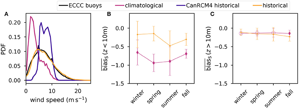
Figure 2. (A) The frequency distribution of wind speeds for the historical period for the daily CanRCM4 climatology (climatological), the CanRCM4 climatology augmented with the daily CanRCM4 anomalies (CanRCM4 historical), and the CanRCM4 climatology augmented with CFSR hourly anomalies (historical). (B,C) Seasonal bias in salinity averaged over all stations at depths (B) < 10 m and (C) > 10 m for a simulations forced with the historical winds and the CanRCM4 climatology. The error-bars represent the standard deviation over the seasonal averages. The diamond markers indicate significant (p < 0.05) differences from the historical simulation (Welch's t-test).

A sensitivity test was conducted using the climatological winds. While this test provides some insight into the influence of high frequency winds, we caution that this was completed during model development and there are small differences in the initial conditions between this run and the historical run. Moreover, we are comparing 1 year of the climatological simulation with a 3 year average from the historical simulation. More details of model validation with shipboard data will be given in section 3.1. For the analysis of the sensitivity test, we binned the vertical profiles at each station into the means above and below 10 m so that the error bars represent the variability across the stations. The solution of the climatological simulation exhibited larger biases in the ocean state compared with the solution of the historical simulation (using the augmented hourly winds) (Figure 2B). In particular, the salinity bias for depths <10 m was significantly reduced (diamond markers) for all of the seasons when high frequency winds were included (Figure 2B). For greater depths, the only significant difference was in fall, however, this cannot be directly attributed to changes in the surface winds because of differences in the initial conditions (Figure 2C). These results suggest that including high frequency wind anomalies is important for an accurate representation of upper ocean mixing.

Some interannual variability is introduced to the wind fields from the CFSR wind speed anomalies. Examining the standard deviation among these 3 years indicates which variables are strongly influenced by upper ocean mixing due to the wind variability. But more carefully conducted model studies are needed to better understand the role that high frequency wind variability plays in setting oceanic conditions for this region. More details of the year-over-year variability for key variables in the 10 year historical simulation are given in section 2.4.

For the future simulations, the same technique of randomly shuffling years for the wind speed anomalies was implemented, but the full range of years from the CFSR data set 1979 − 2010 was used. The randomly selected years used for the wind patterns in RCP 4.5 are 1991, 2003, 2005, 2007, 1979, 1985, 1988, 1999, 1994, 1980, 1987, 2000, and 2008 and for RCP 8.5 they are 1985, 2001, 1998, 2005, 1982, 1989, 2009, 1986, 1993, 1990, 1997, 2002, and 1991.

While the hourly wind frequency is adequate to capture localized wind events, future changes in the frequency, duration, and pathways for these storms are not considered. It is widely accepted that storms tracks will shift poleward in the future as a result of increasing mean ocean temperatures (Yin, 2005). But there is no generally accepted theory about how they will change at regional scales (Shaw et al., 2016; Mbengue and Schneider, 2017), so assessing the impact of changes in weather extremes is beyond the scope of this study.

The magnitude of the wind speeds for the historical simulation (with the CFSR anomaly from 2005) are consistent with climatologies calculated from weather buoy data. The locations of the buoys are shown in Figure 1 and a more complete description of these data is given in the Supplementary Material. The corresponding wind directions are more consistent with the buoys over the open ocean and shelf than near shore (Figure 3). Near the shelf break, winds are typically northward in winter (downwelling-favorable) and to the east or south-east in summer (upwelling-favorable). The wind field is broadly consistent with the observations in terms of the timing of upwelling, but the winds turn too early during the fall transition and too late during the spring transition. Nearer to shore (e.g., buoys 204, 185, 183, 145), the model wind direction has errors of 20–30° (rotated clockwise relative to the observations). The historical winds exhibit more accurate wind speeds and directions than those of the North American Regional Climate Change Assessment Program (NARCCAP) Regional Climate Model (RCM) ensemble (c.f. Figure 5 of Morrison et al., 2014) which were typically rotated counter-clockwise relative to the buoy winds and did not turn sufficiently south during the upwelling season.

FIGURE 3

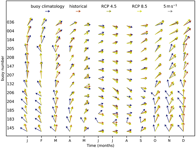
Figure 3. Monthly mean wind vectors for the ECCC buoy climatologies (shown in Figure 1) along with the future and historical wind fields (CanRCM4 and CFSR from 2005).

The year 2005 was used for our comparisons with the future winds because it was common to the random selections for future and historical wind anomalies; the year chosen to provide the high-frequency variability is, however, arbitrary and does not affect the results. Future winds along the shelf begin the spring transition later than the historical winds with a more southward direction during the summer upwelling season (i.e., 204, 206, 207, 132). With the exception of the buoys over the open ocean (004, 036, 184), winds turn earlier in the future during the fall transition (Figure 3).

2.4. Model Spinup

Although the model does not start from rest, it takes some time to adjust to the forcing. Since a different randomly chosen wind anomaly was used for each year, the model was not expected to converge to a perfectly repeating annual cycle. To determine whether the model had equilibrated, the domain was divided into nine different regions and the evolution of essential model variables was evaluated. The spin-up was examined over the entire domain, but we show only the two example regions which are the focus of our study as described below (Figure 1B).

The model resolution varies laterally and vertically. To avoid any biases associated with the variable grid cell volume regional averages for the study regions were normalized using a volume V weighted integral $\overline{F}={\displaystyle {\int }_{V}F}(x,y,z)\frac{dV}{V}.$ The freshwater content is defined by the volume weighted integral of $\frac{S_r-S(x,y,z)}{S_r}$ with a reference salinity S_r = 32.5 and heat content is defined by the volume weighted integral of ρc_p(T(x, y, z) − T_r) where $c_p=4,184\mathrm{\text{ J}}{\mathrm{\text{ kg}}}^{-1}{\mathrm{\text{ K}}}^{-1}$ is the heat capacity of water, ρ = 1,020 kgm⁻³ is a reference density, and $T_r=0^{°}\mathrm{\text{C}}$ is the reference temperature). Both quantities took several years to equilibrate before a regular seasonal cycle was achieved (Figures 4A,B). This adjustment period is most apparent for fresh water (Figure 4B) especially for near surface waters (solid lines).

FIGURE 4

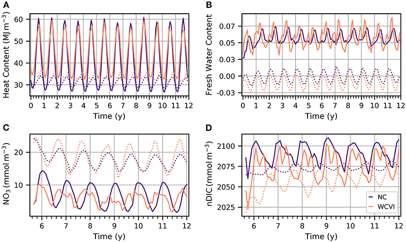
Figure 4. For the historical run, model spinup for the regions shown in Figure 1 (NC, North Coast; WCVI, west Coast Vancouver Island) for depths < 10 m (solid lines) and > 10 m (dotted lines). (A) Ocean heat content, (B) freshwater content and volume weighted mean concentrations of (C) NO₃, and (D) mean DIC concentration normalized to a salinity of S_r = 32.5.

The biogeochemical model was initialized late in year six of the physical model spinup. Volume weighted mean concentrations of NO₃, and the salinity-normalized DIC (nDIC) are shown in Figures 4C,D. Both NO₃ and nDIC undergo substantial adjustments over the first few years before a relatively regular seasonal cycle begins to emerge (Figures 4C,D).

The future simulation was initialized with 3D velocity fields constructed from the ORAS4 data used for the historical simulation, plus CanESM2 anomalies. This simulation exhibited a pattern of convergence for the physical and biogeochemical variables that was similar to the historical simulation (not shown).

3. Results

The analysis focuses on the West Coast of Vancouver Island (WCVI) region and the Northern Coast (NC) region shown by shaded areas in Figure 1B. Both of these regions are bounded by the 500 m isobath on the continental slope. They meet at Brooks Peninsula near the northwestern tip of Vancouver Island. The WCVI region extends south to 47.7° and across the mouth of Juan de Fuca Strait. It is an important region for wind-driven upwelling, and forms the northernmost part of the California Current system.

The NC region substantially overlaps the Pacific North Coast Integrated Management Area (PNCIMA) (Lucas et al., 2007; Irvine and Crawford, 2011), extending to the Alaska/Canada border at the northern edge. The region between Vancouver Island and Haida Gwaii, known as Queen Charlotte Sound, is unique because of its complex bathymetry, with deep troughs along the continental slope and shallow banks that form important habitat for marine ecological communities.

3.1. Model Validation

The model ocean represents a climatology of the historical period (1986–2005) rather than any particular year because it is forced with climatologies of the atmospheric fields (with augmented winds). Therefore, the resulting ocean fields are validated against climatologies estimated from observations over the same period. Generally, the model is in agreement with the observations. The comparisons with the shipboard observations are described in detail and, for brevity, only a summary is given for light-station data, buoy data, and satellite SST analysis, which are further described in the Supplementary Material.

For locations near the coast where the bathymetry is not well resolved, we expected large biases. However, comparisons with the light station data indicate an annual average fresh bias in SSS of about 0.5±0.6 and an average warm bias of around 0.3±0.8°C (Fisheries and Oceans Canada, DFO). The bias for each station and each month are shown in Supplementary Figure 4.

The model exhibits a cold bias in SST of less than 1°C during the winter months transitioning to a warm bias of up to 2°C throughout the summer compared to a climatology of NOAA 1/4° daily Optimum Interpolation Sea Surface Temperature (OISST) (Banzon et al., 2016). The biases appear to be fairly uniform across the domain, whereas we would expect a more spatially variable pattern if the biases were primarily dynamically driven, e.g., the bias would be larger in regions with strong upwelling-favorable winds, which are a small part of the total area. Comparisons with the ECCC buoy SST and SAT suggest that these biases are largely driven by biases in the CanRCM4 surface air temperature (shown in Supplementary Figure 5).

For validation of modeled fields, vertical profiles were compared to shipboard observations at model locations for which there were at least 10 observed vertical profiles within a 5 km radius for each season (winter-DJF, spring-MAM, summer -JJA, fall-SON). To eliminate any overlap, the stations were separated by at least 10 km. The observations were binned to the vertical model levels. For each location and season, model grid points within a 5 km radius were averaged for each z level.

The locations of shipboard observations of ocean temperature and salinity are shown in Supplementary Figure 2. Most of the observations are from the West Coast of Vancouver Island. For all seasons, the model is generally biased cold (Figures 5A–D), with biases typically less than 1°C in summer, fall and winter and slightly larger biases in spring (annual average bias is −0.4±0.6°C). There is a relatively small fresh bias for all of the seasons, with an average bias of −0.2±0.2 (Figures 5E–H).

FIGURE 5

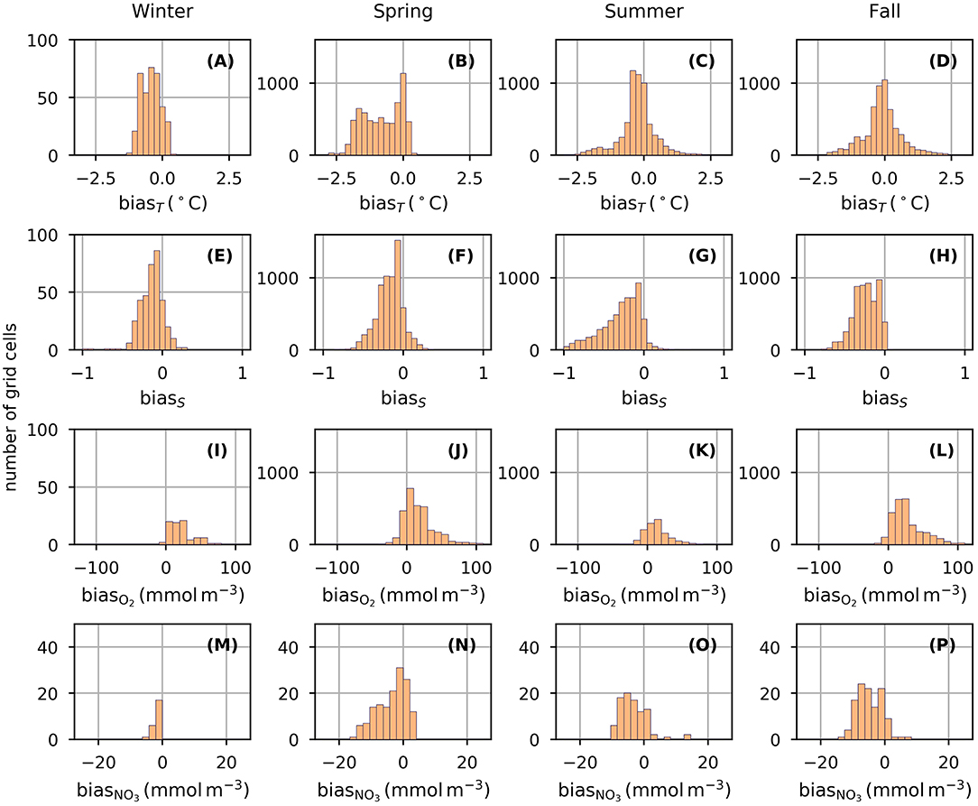
Figure 5. For the historical run, model bias (model-observations) in temperature (A–D), salinity (E–H), oxygen (I–L), and nitrate (M–P) concentration calculated from climatologies of shipboard observations (1986–2005) for each of the seasons as indicated at the top of each column. For T, S, and O₂ the y-axis limits differ for the winter column as there are fewer observations. Relatively few observations of DIC are available so these data were validated using the empirical relationships derived by D. Ianson using the methods and data from Lara-Espinosa (2012) (D. Ianson (Fisheries and Oceans Canada) private communication, 2019) and shown in the Supplementary Material.

The locations of the climatologies for O₂ profiles are primarily focused around WCVI with few in Queen Charlotte Sound. The bias in O₂ is positive for all seasons, with largest values in spring and fall (Figures 5J–M). The mean bias over all of the seasons is about 20 mmolm⁻³ with an average standard deviation of 21 mmolm⁻³.

For NO₃, the locations of available observations were in the WCVI region. The mean bias in NO₃ over all of the seasons is about −3.3 mmolm⁻³ with an average standard deviation of 3.5 mmolm⁻³.

The near-surface salinity bias averaged over all of the stations was significantly reduced by augmenting the climatological winds with high frequency variability from the CFSR winds (Figure 2A). Because randomly selected years were used for the CFSR wind anomaly, this result indicates that exact knowledge of the high-frequency variability is not required to substantially reduce model bias. It is evident from the sensitivity test that the nonlinear response of ocean surface currents and mixing/stirring to high-frequency wind forcing is important to accurately simulating the freshwater distribution in this region.

3.2. Broad Changes Across the Continental Shelf

Both the NC and WCVI regions are projected to experience substantial changes. To illustrate the annual changes along the Northeastern Pacific continental shelf in the 2055 climate, Figure 6 shows the volume weighted averages for several model variables. Error bars correspond to the standard deviation across the 3 years averaged (which is due to the variability in the winds).

FIGURE 6

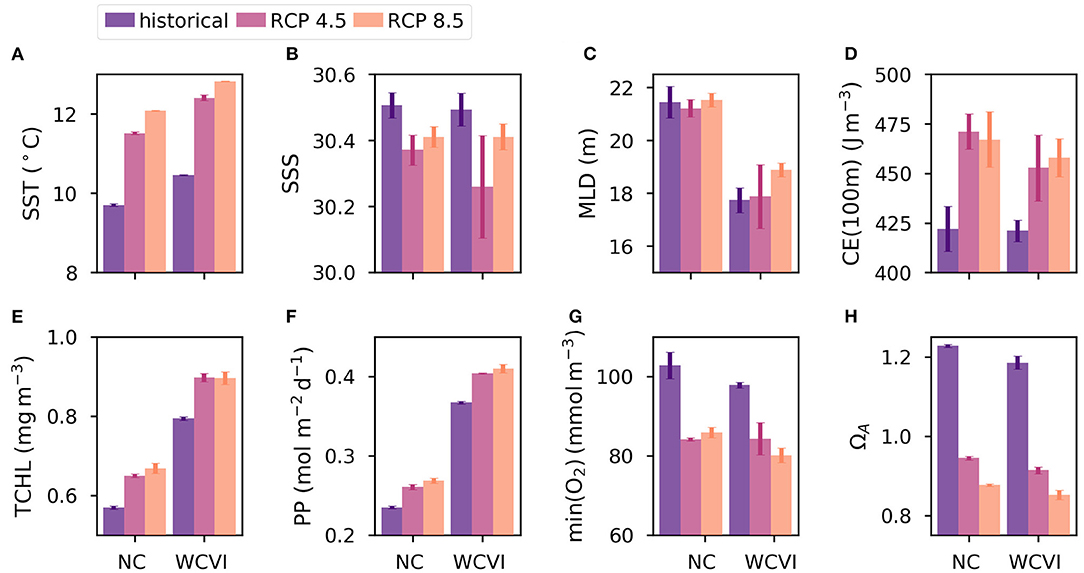
Figure 6. Annual average (A) sea surface temperature, (B) sea surface salinity, (C) mixed layer depth, (D) convective energy, (E) total chlorophyll, (F) primary productivity, and volume weighted averages over the bottom 100 m for (G) minimum oxygen, and (H) aragonite saturation state for historical (1986-2005) and future (2045-2065) simulations. Error bars represent the year-to-year variability due to the wind stress anomaly.

The regionally averaged SST is projected to increase by 1.8°C for the NC and 2.0°C for WCVI under RCP 4.5 and by 2.4°C for both regions under RCP 8.5 (Figure 6A). These increases correspond to a change between 3°C and 4°C per century which is more rapid than the 0.9°C per century increase reported by Cummins and Masson (2014) for BC lightStations over the historical record (60–70 years).

The average SSS decreases by −0.14 in the NC region and by −0.23 in WCVI for RCP 4.5, yet for RCP 8.5, SSS decreases by −0.10 for the NC and −0.08 for WCVI (Figure 6B). While the change appears to be greater in RCP 4.5, the difference is smaller than the interannual variability associated with the augmented wind forcing which strongly influences the freshwater distribution. The variability among model years due to augmented wind forcing is considerably larger for SSS than for SST, but still smaller than the change. While the future projections all indicate freshening which is likely due to increases in precipitation, the magnitude of the difference is less well-constrained due to uncertainties in the projected wind speed distributions for 2046–2065.

The only clear change in mixed layer depth (Figure 6C) is a projected increase for WCVI under RCP 8.5; year-to-year variability due to the wind anomaly is substantial. The overall stratification of the water column increases. The convective energy (CE), the amount of energy required to mix the column to a given depth (100 m), is projected to strengthen for both regions with a greater increase in the NC compared with WCVI (Figure 6D). This increase of about 50Jm⁻³ is relatively small, yet it represents an ≃ 10% increase in stratification. The static stability of the water column is controlled primarily by the salinity in all of the simulations (not shown). The increase in stratification does not appear to inhibit phytoplankton growth, as total chlorophyll and primary productivity increase for both of the regions (Figures 6E,F).

The minimum oxygen and average aragonite saturation state (Ω_A) below 100 m decreases for both regions indicative of more corrosive (lower Ω_A) and less oxygenated waters on the continental shelf (Figures 6G,H). Error bars confirm that the wind anomaly influences minimum oxygen concentration on the shelf as highly oxygenated near-surface waters are mixed downward, but has little effect on Ω_A.

There is a relatively low amount of hypoxic (< 60 mmolm⁻³) water in the study regions on the continental shelf, but the volume (weighted by the volume of each grid cell) increases from around 5 km³ in the historical simulation to around 50 km³ by the 2050s (Supplementary Figure 6). The volume of undersaturated waters is much higher (≃ 1,000 km³). Throughout the year, the largest volume of corrosive water is in the NC region, while the largest volume of low-oxygen water is in the WCVI region. The oxygen minimum zone is deeper in the northern part of the domain (discussed in section 3.3) so less of the low-oxygen water flows onto the shelf. Since the saturation horizon is higher in the water column than the oxygen minimum zone, corrosive water flows into the deep sub-marine canyons of the NC more than in the WCVI region (see Supplementary Figure 1).

During summer upwelling, the aragonite saturation state of shelf waters is generally lower than the other seasons (Supplementary Figure 6). Maps of the minimum summer Ω_A illustrate that while minimum Ω_A does not change very much in the open ocean, the shelf regions are becoming undersaturated (Ω_A < 1) (Figure 7) even for the moderate mitigation scenario RCP 4.5. Hotspots of change include the near shore regions of WCVI and the banks of the NC (Figure 7C). For RCP 8.5, the magnitude of the change is greater, but the locations of greatest change remain similar to RCP 4.5. While the maps illustrate changes east of Vancouver Island (the Salish Sea), we have neglected this region because even 2 − 3 km resolution is not adequate there (cf. Peña et al., 2016; Soontiens and Allen, 2017).

FIGURE 7

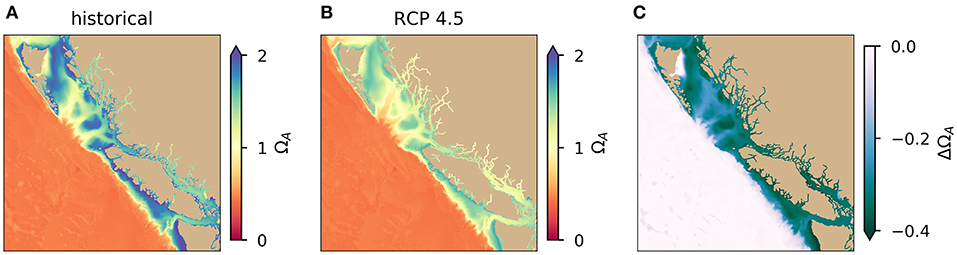
Figure 7. Maps of the minimum aragonite saturation state in summer for the (A) historical period, (B) future (RCP 4.5), and the (C) difference between the two. Here the 5-day averages were used to compute Ω_A and the minimum was taken over all depths.

The key factors influencing phytoplankton growth and primary productivity are light, temperature, availability of nutrients (in this region principally N), and stratification of the water column. There is a notable increase in Total Chlorophyll (TCHL) in the top 10 m across the continental shelf. For example, Figures 8A,B shows the volume averaged change in TCHL for RCP 4.5. Surface chlorophyll is strongly affected by wind variability (shaded regions showing standard deviation due to the wind anomaly) especially during the spring over WCVI. Fewer nutrients reach the euphotic zone in the future scenarios, but subsurface nitrate is projected to increase during the upwelling season (Figures 8C,D) which may be a consequence of stronger upwelling winds. The non-dimensional nitrogen limitation term (N_lim) is based on the cell N quota; it ranges between 0 and 1 with larger values corresponding to increased growth rates (Hayashida et al., 2019). Although the stratification is increasing, nitrogen limitation does not appear to be a major factor limiting productivity along the continental shelf in the 2050s (Figures 6F,G). Since nutrient concentrations are generally sufficient to support phytoplankton growth, increases in productivity across the continental shelf could be due to temperature dependent metabolic rate, changes in the mixed layer depth, or changes in circulation. More work is needed to understand these mechanisms.

FIGURE 8

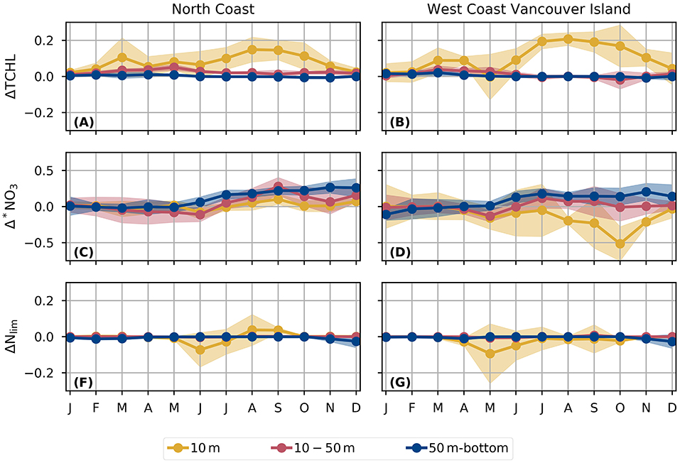
Figure 8. Regionally averaged changes between 1986 − 2005 and 2046 − 2065 (RCP 4.5) for (A), (B) total chlorophyll (C), (D) nitrate concentration (normalized by the range of values in the historical period) and (F), (G) nitrogen limitation of phytoplankton based on cell nitrogen quotas. Shaded regions correspond to the standard deviation among the years averaged due to wind variability as in Figure 6. Nitrogen limitation is a non-dimensional index ranging from 0 (cell quota at its minimum) to 1 (cell quota at its maximum).

3.3. Changes Along the Continental Slope

Figure 9 shows a vertical cross-section across WCVI (the green line in Figure 1). Each column corresponds to a different simulation. Qualitatively, impacts are similar for both scenarios from the continental shelf to the shore; isopycnal surfaces are deepening, while corrosive, deoxygenated water is rising. For RCP 8.5 the effect is more pronounced with corrosive waters moving to shallower depths in the water column (Figure 9 row 2 and 3). While the oxygen content is declining for the bottom waters across the continental shelf, maps of the spatial extent indicate that hypoxic waters remain largely confined to the continental slope (not shown).

FIGURE 9

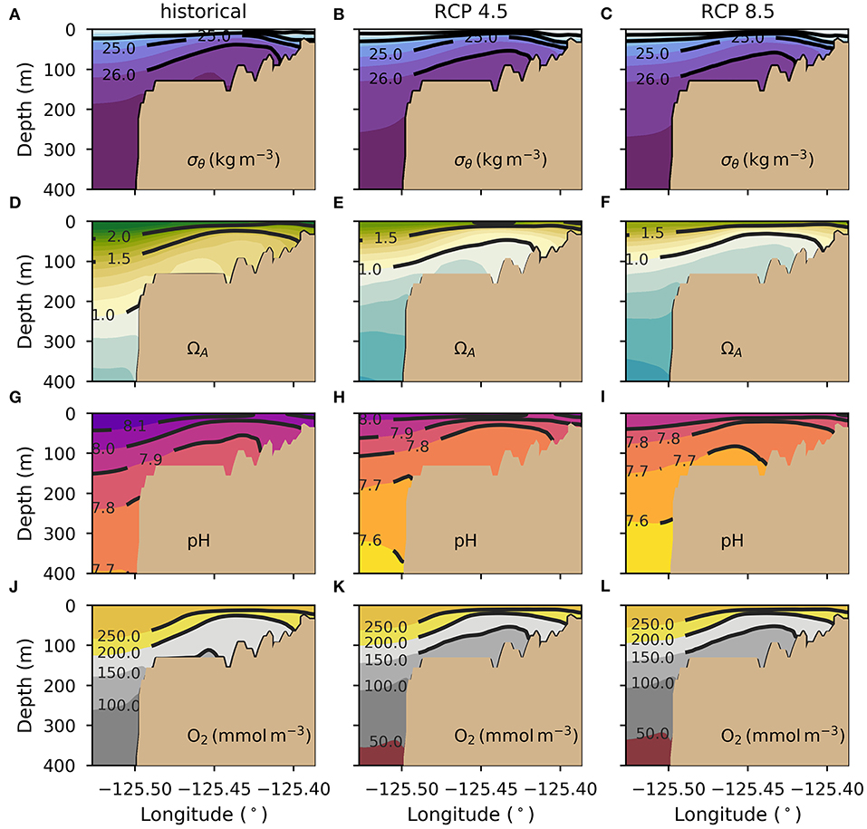
Figure 9. Vertical cross-sections taken across WCVI (green line in Figure 1B) of the summer climatology for (A–C) potential density (color contours every 0.5σ_θ), (D–F) aragonite saturation state (color contours separated by 0.1), (G–I) pH and (J–L) dissolved oxygen. Each column corresponds to the simulation indicated on the top panel (historical, RCP 4.5 and RCP 8.5).

To estimate the projected changes along the continental margin, we first located the 300 m isobath for both focus regions, then moved approximately 100 km along the model grid toward the open ocean (purple markers in Figure 10A). Seasonally averaged fields were extracted along this vertical cross-section and interpolated to a uniform 1 m vertical grid.

FIGURE 10

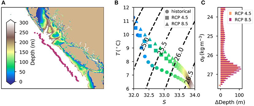
Figure 10. Changes in the depths of isopycnal surfaces for a series of locations (100 km seaward of the 300 m isobath. (A) Locations of vertical profiles and bathymetry for depth < 300 m. (B) T-S plots for present and future with depth of isopycnal indicated by color (same colorbar as A), and (C) change in the depth of isopycnals between present and future simulations. All results are summer climatologies, averaged over all of the locations shown in (A).

Isopycnal surfaces (binned at a resolution of 0.1σ_θ) are projected to deepen with increased temperature and salinity at a given density (e.g., Figure 10B). In summer, isopycnals are located deeper in the water column by as much as 100 m depending on the isopycnal (Figure 10C). For all of the seasons, the most pronounced changes in isopycnal depth are from 26σ_θ to 27σ_θ (i.e., below the pycnocline), where the vertical density gradient is small. Nearer to the surface, there are seasonal differences in the T-S plots. In summer and fall warming isopycnals deepen by between 15 and 25 m, while increased precipitation in winter and spring results in near-surface isopycnals that are warmer and fresher with deepening by 15–60 m (not shown).

A likely mechanism driving the apparent downward “shift” of isopycnal surfaces is warming and freshening from the surface downward, which decreases the density at a specific depth horizon causing a downward relocation of the isopycnal. That this mechanism is responsible for the relocation is evident from, for example, the average temperature and salinity profiles for summer (Figure 11). Anthropogenic warming produces a warmer atmosphere with higher levels of precipitation in the 2050s. The warming signal propagates downward through the water column, with warming up to 2°C near the surface tapering off to 1°C at 500 m depth (Figure 11A) increasing the stratification. Substantial freshening due to increases in precipitation reduces the density at the surface, and the salinity anomaly is mixed down into the upper water column (Figure 11B). In effect, both future scenarios have lighter density waters near the surface than the historical simulation which results in the “movement” of denser isopycnals to greater depth (Figure 11C). This result is consistent with observations of T, S, and P from the 1970s to 1990s which show a downward displacement of density surfaces at latitudes between 45° and 50° (Helm et al., 2011).

FIGURE 11

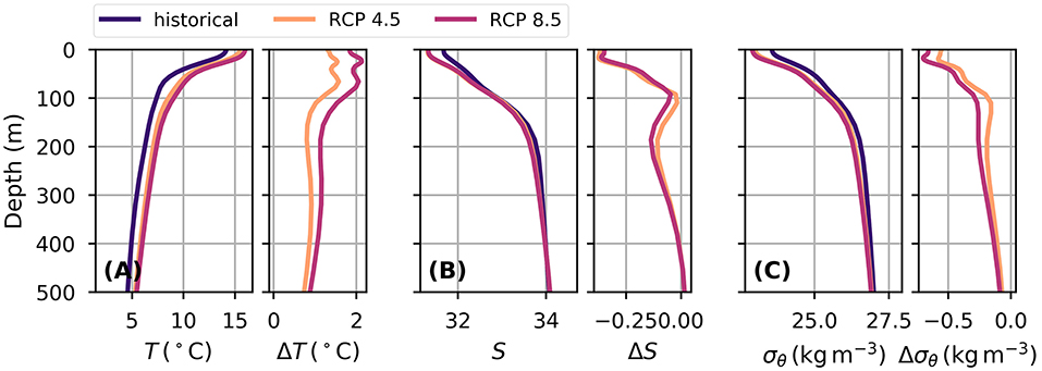
Figure 11. Using the same summer-averaged vertical profiles that were used in Figure 10 the average profiles are shown for each simulation with differences (future-historical) on the right panel for (A) temperature, (B) salinity, and (C) density.

The change in oxygen near the surface can be attributed mainly to changes in solubility (controlled primarily by temperature), while changes along deeper isopycnals are primarily due to changes in remineralization and circulation. The apparent oxygen utilization was calculated by subtracting the actual concentration from the saturation value of oxygen (i.e., AOU = [_O2]sat − [O₂]). Assuming the non-solubility fraction is entirely due to remineralization (remin = − AOU), the remineralization component for DIC and NO₃ were also estimated (Sarmiento and Gruber, 2006). For example, Figure 12 shows the change along isopycnal surfaces for summer climatologies near the continental slope (locations shown in Figure 10A). The change due to solubility is relatively small for the near-surface isopycnals (σ_θ < 25), but this figure excludes isopycnals that are not present in the historical climate because of substantial decreases in surface density (i.e., Figure 11C). If, instead, the solubility fraction is calculated based on depth levels (e.g., inset panel of Figure 12), it accounts for about 84% (94%) of the total in the upper 100 m and 21% (28%) over all depths for RCP 4.5 (RCP 8.5). These values are larger than the observed oxygen decline due to solubility since the 1960s of ≃ 15% for the global ocean (Helm et al., 2011; Schmidtko et al., 2017).

FIGURE 12

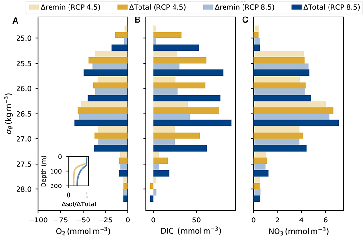
Figure 12. For isopycnals (binned at a resolution of 0.5σ_θ), the (A) total change in [O₂] and the change that is not attributable to solubility (remin = −AOU). The inset panel shows the fraction of the change in [O₂] that is due to solubility for each depth. Total change and estimated changes due to remineralization for (B) DIC and (C) nitrate. The remineralization fraction was calculated from AOU assuming 1O₂:1C:(16/106)N. All results are based on summer climatologies averaged over all of the locations shown in Figure 10A.

The largest declines in oxygen occur for isopycnals between 26σ_θ and 27σ_θ because that is where the most substantial relocation occurs. For example, in summer under RCP 4.5, the greatest changes in concentration occur for σ_θ = 26.5 with $\Delta {\mathrm{\text{O}}}_2=-54\mathrm{\text{mmol}}{\mathrm{\text{m}}}^{-3}$ and correspond to a depth change of ≃ 70 m. Comparing this to the vertical gradient of O₂ in the historical climate, we find that if σ_θ = 26.5 were to be displaced downward by the same distance then $\Delta {\mathrm{\text{O}}}_2\simeq -55\mathrm{\text{mmol}}{\mathrm{\text{m}}}^{-3}$. This simple example demonstrates that the magnitude of the change in concentration on specific isopycnals experience is broadly consistent with the downward displacement of the isopycnal surfaces.

Crawford and Peña (2013) examined the decline off of WCVI for σ_θ = 26.6 from 1981 to 2011. While direct comparisons with their observations are not possible because of differences in sampling and model bias, examining the same isopycnal provides insight into the change in O₂ for the region. On average, the σ_θ = 26.6 isopycnal sits at a depth between 186 m and 296 m in the historical simulation with an average oxygen concentration of 122 mmolm⁻³. The change of about −0.9 mmolm⁻³ y⁻¹ (−1.0 mmolm⁻³ y⁻¹) for RCP 4.5 (RCP 8.5) (estimated from the two time-slices) is broadly consistent with the declines (Crawford and Peña, 2013) estimated over the historical period.

The downward penetration of atmospheric CO₂ into the water column is responsible for most of the change in the DIC. The change due to remineralization, estimated from AOU (DIC_rem), is small relative to the total projected change especially near the surface (Figure 12B). DIC_rem only approaches half of the total change at the isopycnals where O₂ change is greatest (Figure 12). The change in DIC due to anthropogenic CO₂ is likely to be primarily local, because it declines approximately monotonically from the surface down, because it is consistent across the region (not shown), and because vertical penetration will be generally slower in oceanic waters, making an explanation based on subsurface advection of such waters unlikely. The remineralization fraction may be partly local and partly advective (given the horizontal gradients in concentration, it would take only a fairly small change in mean circulation to explain the changes in concentration, and the stoichiometry of O₂ loss / DIC and NO₃ gain would be similar). However, a primarily advective mechanism is unlikely because of the small change in salinity at the levels where the greatest change occurs (Figures 10, 11), and because, as noted above, the change in O₂ on e.g., 26.5 is consistent with the downward displacement of the isopycnal by surface warming and freshening. To the extent that the change in salinity is not monotonic with depth, the deviation occurs at much shallower depths (Figure 11) and is most plausibly explained by shoreward advection of more oceanic water due to slightly stronger upwelling-favorable winds.

For nitrate, most of the change is associated with remineralization (Figure 12C). The increase in remineralization is attributed primarily to the relocation of the isopycnal surfaces, as DIC and nitrate both increase monotonically with depth.

Corrosive (undersaturated) waters are projected to encroach substantially on the continental shelf. The average aragonite saturation state decreases by 0.2 (0.3) in RCP 4.5 (RCP 8.5) (Figure 14A) becoming consistently undersaturated throughout the year.

The oxygen minimum zone is projected to rise up in the water column by about 75 m. For example, Figure 13 shows the change in the depth of the 60 mmolm⁻³ isopleth (locations in Figure 10A) under RCP 4.5. The dashed line marks Brooks Peninsula which separates the WCVI and NC regions as discussed above. The depths vary seasonally, particularly for the NC region; deeper during winter downwelling and shallower during summer upwelling. The isopleth shoals more in the south than in the north. Qualitatively similar results were found along the 300 m isobath (parallel to those shown in Figure 10A), but there was much more variability along the transect (not shown). Shaded regions indicate the variability associated with the wind anomaly was ±27 m.

FIGURE 13

Figure 13. Depth of the $\left[{\mathrm{\text{O}}}_2\right]=60\mathrm{\text{ mmol}}{\mathrm{\text{m}}}^{-3}$ isopleth for historical and future simulations in (A) winter, (B) spring, (C) summer, and (D) fall for a series of vertical profiles along the 300 m isobath of the continental shelf (parallel to the locations in Figure 10).

The annual change in potential temperature for a transect along the 300 m isobath is 0.9°C (1.8°C) in RCP 4.5 (RCP 8.5) which represents an average change of about 1.5°C (2°C) per century. The depth of the saturation horizon along that transect shoals by about 100 m across all seasons (Figure 14B) while exhibiting the same seasonal cycle of a shallower (deeper) horizon during the upwelling (downwelling) seasons. The encroachment projected over the next 50 years is substantially larger than the change observed since the preindustrial period of 30–50 m (Feely et al., 2016).

FIGURE 14

Figure 14. For a series of vertical profiles along the 300 m isobath of the continental shelf (parallel to the locations in Figure 10), the average (A) aragonite saturation state and (B) saturation horizon for each month.

In summer in the future simulation, corrosive waters reach into the top 100 m of the water column along the continental slope. Stronger summer upwelling is not the primary driver of the change in acidification as isopycnal surfaces are deeper in the future relative to the historical period. Instead the change is driven primarily by downward mixing of anthropogenic DIC.

3.4. Extreme States

Because extreme states are known to have important biological impacts that can be overlooked by looking only at mean states, we recorded the maximum and minimum values within the 5 day averaging period. A series of vertical profiles are extracted along the 300 m isobath of the continental slope (parallel to the locations in Figure 10) to examine how extreme states are changing. For each grid cell, the minimum (maximum) value for each season is used in the histogram. Broadly, extreme states of corrosive and deoxygenated water are becoming more frequent and more extreme, and extremely cold temperatures are becoming rare (Figure 15). The peak of the pH histogram is shifting to more acidic conditions, with a noticeably greater effect in RCP 8.5 than RCP 4.5. For oxygen, Figure 15B is truncated to emphasize hypoxic states, but the mode for the historical simulation is around 290 mmolm⁻³, which declines by 13 − 20 mmolm⁻³ in the future scenarios. Roughly 6% of the [O₂] data are below the canonical hypoxic threshold of 60 mmolm⁻³, whereas in RCP 4.5 (RCP 8.5) more than 11% (12%) are below this threshold (Figure 15B). The modal minimum temperature in the historical simulation is 7°C increasing by between 1.9°C and 2.4°C by the 2050s. In the historical simulation around half of the temperatures are below 7°C, but this declines to less than 23% (21%) in RCP 8.5 (RCP 4.5) (Figure 15C).

FIGURE 15

Figure 15. Annual minimum (A) pH, (B) oxygen concentration, and (C) temperature and (D) annual maximum temperature for vertical profiles along the 300 m isobath parallel to those shown in Figure 10A. For oxygen, the x-axis has been truncated to emphasize the increase in frequency of concentrations below 60 mmolm⁻³.

States of extremely warm temperatures are increasing in magnitude and frequency (Figure 15D). The maximum temperature in the historical climate was 17.8°C increasing to 18.9°C (19.9°C) by the 2050s in RCP 4.5 (RCP 8.5). At that time, about 4% (15%) of maximum temperatures will be above the historical extreme maximum temperature of 17.8°C.

4. Discussion

Warming and freshening at the ocean surface will propagate throughout the water column on the continental shelf as these waters are mixed vertically by winter storms and tidal currents. Increased carbon dioxide absorbed from the atmosphere is also mixed throughout the water column, moving the CaCO₃ saturation horizon upward and onto the continental shelf. pH declines substantially, with corrosive bottom waters present in both study regions. Beyond the continental shelf, there is gradual downward penetration of excess heat and DIC that results in shoaling of the isopleths of oxygen concentration and CaCO₃ saturation state (e.g., Figure 9). Shoaling of corrosive and oxygen poor waters gives rise to new potential impacts, as these waters can affect the biota of the continental shelf, especially during upwelling events and storms.

Our experiments help to elucidate a dominant mechanism by which changes in thermocline biogeochemistry along the continental slope occur. There is no evidence of enhanced “uplift” of isopycnal surfaces due to changes in wind stress. Rather, the isopycnal surfaces are relocated to greater depths as warm and fresh surface inputs are mixed downward, reducing the density at each depth stratum. This mechanism is thermodynamic rather than dynamic and changes the biogeochemistry associated with each isopycnal.

This study provides an overview of the projected climate impacts for the continental shelf focusing on general impacts for a large geographical area that has complex bathymetric features (Supplementary Figure 1) and circulation. Projected changes in advection, upwelling, and downwelling have variable impacts across the continental slope so the analysis presented here does not preclude changes in the circulation for the region. Further study of the localized impacts using higher resolution coastal models is warranted.

By examining the change in oxygen concentration and its deviation from that expected from saturation concentration alone, we can estimate the remineralization contribution to changes in nitrate and DIC. Remineralization dominates changes in nitrate concentration on specific isopycnal surfaces, mainly because the concentration increases with depth and there is a relocation of isopycnal surfaces. Changes in DIC are dominated by the downward penetration of anthropogenic CO₂. As previously noted by Feely et al. (2008), whatever other changes in circulation or remineralization occur that affect e.g., the CaCO₃ saturation state, will be exacerbated by the contribution of anthropogenic CO₂.

An important limitation of this study is that runoff data for the future climate simulations were not available. Changes in surface freshwater flux are therefore solely due to evaporation and precipitation. This bias is likely to be small along the WCVI during the summer upwelling season, as runoff is mostly precipitation driven and is low in summer. It is potentially larger in the NC where runoff from melting snowpack plays a larger role. If summer runoff declines substantially, it could make the water column more unstable and lead to entrainment of deeper oxygen poor or low pH into the surface layer in some regions. In our experiments, the change is toward slightly greater stratification (Figure 6), but this is a broad regional average. Less springtime runoff along the WCVI region could result in a less stable water column as the near-surface salinity is lowest during spring (Figure 4).

Because of the augmented winds, this study provides evidence that the high-frequency variability in the wind stress is essential to realistically distributing the freshwater sources throughout the model domain (e.g., Figure 2). Variations in the annual pattern of high frequency wind stress, such as gale force winds and storms, modify mixed layer depths, and the near surface stratification (e.g., Figure 6) and affect the amount of nutrients reaching the surface (e.g., Figure 8). The variability of the winds also influences the depth of the oxygen minimum zone along the continental shelf through its influence on the ocean circulation (e.g., Figure 13), but has little effect on ocean acidification despite its influence on gas exchange (e.g., Figure 14).

On the whole, total chlorophyll and primary productivity increase (Figures 6, 8), and this is universally the case over a larger set of smaller averaging regions (not shown). But we caution that the biological model was developed for the global domain and was applied to these simulations with no parameter tuning. The main influence on phytoplankton production is increased temperature, as the region is relatively replete with nutrients and has shallow mixed layers. Again, we generally expect stratification to increase, although the opposite may occur locally in some runoff-dominated regions. There is a slight increase in N stress in some seasons (Figure 8). In general, we do not expect any decline in productivity over the time scale considered here, although we can not rule out changes in species composition. Any increase in N limitation is of concern in a region dominated by diatoms adapted to nutrient-rich environments.

This study has shown that future climate under either scenario exhibits more frequent and more extreme states of warm temperature, hypoxia and acidification. While changes in each of these stressors individually have important consequences for ecosystem health, simultaneous shifts in these three stressors can result in synergistic effects that greatly exceed the effect of each in isolation (Gruber, 2011). Together they threaten marine biodiversity and ecosystem health by inhibiting growth, respiration, reproduction, and immune response as well as causing epigenetic changes in organisms (Haigh et al., 2015; Breitburg et al., 2018). More work is needed to understand the durations, magnitudes, and locations of extreme events and their impacts on ecosystems.

Our results are constrained between the bounds of the two scenarios examined. While RCP 8.5 is the scenario with the least mitigation, RCP 4.5 provides a more conservative estimate of the extent of changes to marine ecosystems that will occur by the 2050s. RCP 2.6 has even lower emissions than RCP4.5, but it is unlikely to be achieved given the amount of CO₂ that has already accumulated in the atmosphere (Arora et al., 2011). A newer set of scenarios, and simulations conducted with them, are now available via CMIP6, but are unlikely to substantially alter the results shown.

This study has explored scenario uncertainty by looking at RCP 4.5 and RCP 8.5. After scenario uncertainty, model uncertainty is the next largest source of error (Frölicher et al., 2016). To minimize this uncertainty, a range of climate models (in addition to CanESM/CanRCM) should be explored; we are presenting initial results from a single-model downscaling study because the cost of ensembles is presently prohibitive. The third source of uncertainty is natural variability (Deser et al., 2012; Cheung et al., 2016); because our experimental design uses climatological forcing for each time period, the differences are almost entirely due to anthropogenic forcing with little effect of natural variability. However, we caution that our experimental design does not permit us to address the effects that physical processes underlying natural climate variability in this region may have on future changes in ocean state.

The method for downscaling atmospheric climatologies presented here introduced high frequency variability to the climatological winds. Consequently, a relatively small amount of interannual variability was also introduced to the model solution through the wind fields. Examining the standard deviation among these years is a useful hueristic for exploring the role of the high frequency wind variability in the setting the physical and biogeochemical oceanographic properties for the North-Eastern Pacific continental margin. To analyze the projected changes for the region we averaged the last 3 years of the model solution. The historical simulation represents the climate from (1986 to 2005) with an acceptable bias (Figure 5). All of the model solutions converge toward a repeating annual cycle after several years of spinup (Figure 4). Therefore, the difference between the historical and future climates is much larger than the interannual variability introduced through the high frequency wind speed variability.

Forcing the model with climatological means (time-slice approach) instead of running the model continuously through the historical and future period reduces computational expense, but it also limits the breadth of climate information that can be provided. Estimates of “the rate of change” for modeled variables presented in this paper are broad estimates using only two points in time.

5. Conclusions

This paper has examined climate change projections along the continental shelf of the Canadian Pacific Coast by dynamically downscaling using the North-Eastern Pacific Canadian Ocean Ecosystem Model (NEP36-CanOE). To circumvent computational constraints, a new approach was introduced that downscales using atmospheric climatologies (with augmented winds) to project ocean circulation and biogeochemistry under moderate mitigation (RCP 4.5) and high emissions (RCP 8.5) scenarios.

Comparisons with available observations showed that the time-slice approach was able to reproduce the observed climate state for the historical period. The model exhibited a cold bias that was typically less than 1°C (annual average bias is −0.4 ± 0.6°C) and a freshwater bias of −0.2 ± 0.2 when compared to shipboard observations. Including high-frequency wind forcing reduces the salinity bias substantially and does not require specific knowledge of how this component may change.

Over the 60 year period between the historical and future climates, surface ocean temperatures will increase across the NC and WCVI by between 1.8°C and 2.4°C depending on whether a moderate or high emissions scenario is used. The projected surface freshening is between −0.08 and −0.23, however future changes in fresh water content will be strongly affected by changes in wind stress. Changes in wind stress have a substantial influence on freshwater distribution, and wind speeds may change in the future in ways not fully captured by the RCM.

Stratification, primary production and total chlorophyll are increasing along the continental margin and across the continental shelf. There is some evidence of increased nutrient limitation in summer and changes in species composition are possible (e.g., a shift from diatoms to dinoflagellates, including harmful algal bloom species), but our results suggest that changes in overall productivity will be small over this time scale.

Low CaCO₃ saturation state (corrosive) and low oxygen waters are projected to rise up the continental shelf. In the 2055 climate, the saturation horizon and oxygen minimum zone are projected to rise by ≃ 100 m and ≃ 75 m, respectively, relative to the historical simulation. With corrosive and hypoxic waters nearer to the surface, episodes of extremely acidic and deoxygenated water become more likely along shorelines and in regions important to fisheries and aquaculture and other marine life.

By examining the maximum and minimum values within the 5 day averaging period, we showed that extreme states of hypoxic, corrosive and warm water are projected to become more frequent and more extreme. In addition, extremely cold temperatures are becoming rare.

The increase in temperature and acidity projected by the 2050s for both scenarios is substantially greater than the change observed over the historical record (Cummins and Masson, 2014; Feely et al., 2016) because increasing GHGs in the atmosphere are accelerating the rate of change. Over this time-scale, there is little difference in ocean acidification or deoxygenation between the moderate mitigation scenario (RCP 4.5) and the high emissions scenario (RCP 8.5).

Data Availability Statement

The data associated with this work is publicly accessible using the following link: Northeastern Pacific Canadian Ocean Ecosystem Model (NEP36-CanOE) Climate Projections – https://open.canada.ca/data/en/dataset/a203a06d-9c1f-4bb1-a908-fc52912ff658.

Author Contributions

AH adapted the biogeochemical model for use in NEMO 3.6, developed the forcing fields including the downscaling methodology (augmented winds), conducted the climate simulations, validated the model, developed analysis methodology and completed analysis, interpreted results, and wrote the manuscript. LZ developed and tuned the physical model, assisted with debugging for the BGC model, contributed to the final version of the manuscript. YL led the development of the physical model, contributed to the final version of the manuscript (particularly with refining the write up for the methodology). JC principle investigator for the project, had the initial idea for the project and supervised the work, advised on the development of methodology, contributed to the interpretation of the results, and edited the manuscript. All authors contributed to the article and approved the submitted version.

Funding

This work was supported by the Fisheries and Oceans Canada's (DFO) Aquatic Climate Change Adaptation Services Program (ACCASP).

Conflict of Interest

The authors declare that the research was conducted in the absence of any commercial or financial relationships that could be construed as a potential conflict of interest.

Acknowledgments

We are grateful to all of the DFO and ECCC staff who have collected at-sea observations, and other observational data sets such as the weather buoys and lighthouse stations, over many years, and to those responsible for the CanRCM model output. We also thank the originators of all of the public-domain data products used, including GLODAP, WOA, OISST, and CFSR. Thanks to Adam H. Monahan, for useful discussions about the augmented wind forcing.

Supplementary Material

The Supplementary Material for this article can be found online at: https://www.frontiersin.org/articles/10.3389/fmars.2021.602991/full#supplementary-material

Footnotes

1. ^http://sosie.sourceforge.net/

2. ^http://www.bio.gc.ca/science/research-recherche/ocean/webtide/index-en.php

References

Arguez, A., and Vose, R. S. (2011). The definition of the standard [WMO] climate normal: the key to deriving alternative climate normals. Bull. Am. Meteorol. Soc. 92, 699–704. doi: 10.1175/2010BAMS2955.1

CrossRef Full Text | Google Scholar

Arora, V. K., Scinocca, J. F., Boer, G. J., Christian, J. R., Denman, K. L., Flato, G. M., et al. (2011). Carbon emission limits required to satisfy future representative concentration pathways of greenhouse gases. Geophys. Res. Lett. 38:L05805. doi: 10.1029/2010GL046270

CrossRef Full Text | Google Scholar

Balmaseda, M. A., Mogensen, K., and Weaver, A. T. (2013). Evaluation of the ECMWF ocean reanalysis system ORAS4. Q. J. R. Meteorol. Soc. 139, 1132–1161. doi: 10.1002/qj.2063

CrossRef Full Text | Google Scholar

Banzon, V., Smith, T. M., Chin, T. M., Liu, C., and Hankins, W. (2016). A long-term record of blended satellite and in situ sea-surface temperature for climate monitoring, modeling and environmental studies. Earth Syst. Sci. Data 8, 165–176. doi: 10.5194/essd-8-165-2016

CrossRef Full Text | Google Scholar

Barton, A., Waldbusser, G. G., Feely, R. A., Weisberg, S. B., Newton, J. A., Hales, B., et al. (2015). Impacts of coastal acidification on the Pacific Northwest shellfish industry and adaptation strategies implemented in response. Oceanography 28, 146–159. doi: 10.5670/oceanog.2015.38

CrossRef Full Text | Google Scholar

Bishop, J. K. B., Rossow, W. B., and Dutton, E. G. (1997). Surface solar irradiance from the international satellite cloud climatology project 1983-1991. J. Geophys. Res. 102, 6883–6910. doi: 10.1029/96JD03865

CrossRef Full Text | Google Scholar

Breitburg, D., Levin, L. A., Oschlies, A., Grégoire, M., Chavez, F. P., Conley, D. J., et al. (2018). Declining oxygen in the global ocean and coastal waters. Science 359:6371. doi: 10.1126/science.aam7240

PubMed Abstract | CrossRef Full Text | Google Scholar

Cannaby, H., Fach, B. A., Arkin, S. S., and Salihoglu, B. (2015). Climatic controls on biophysical interactions in the black sea under present day conditions and a potential future (A1B) climate scenario. J. Mar. Syst. 141, 149–166. doi: 10.1016/j.jmarsys.2014.08.005

CrossRef Full Text | Google Scholar

Chan, F., Barth, J.A., Kroeker, K. J., Lubchenco, J, and Menge, B. A. (2019). The dynamics and impact of ocean acidification and hypoxia: insights from sustained investigations in the Northern California Current Large Marine Ecosystem. Oceanography 32, 62–71. doi: 10.5670/oceanog.2019.312

CrossRef Full Text | Google Scholar

Cheung, W. W., Frölicher, T. L., Asch, R. G., Jones, M. C., Pinsky, M. L., Reygondeau, G., et al. (2016). Building confidence in projections of the responses of living marine resources to climate change. ICES J. Mar. Sci. 73, 1283–1296. doi: 10.1093/icesjms/fsv250

CrossRef Full Text | Google Scholar

Cheung, W. W., Lam, V. W., Sarmiento, J. L., Kearney, K., Watson, R., Zeller, D., et al. (2010). Large-scale redistribution of maximum fisheries catch potential in the global ocean under climate change. Glob. Change Biol. 16, 24–35. doi: 10.1111/j.1365-2486.2009.01995.x

CrossRef Full Text | Google Scholar

Christian, J. R. (2014). Timing of the departure of ocean biogeochemical cycles from the preindustrial state. PLoS ONE 9:e109820. doi: 10.1371/journal.pone.0109820

PubMed Abstract | CrossRef Full Text | Google Scholar

Crawford, W. R., and Pe na, M. A. (2013). Declining oxygen on the British Columbia continental shelf. Atmos. Ocean 51, 88–103. doi: 10.1080/07055900.2012.753028

CrossRef Full Text | Google Scholar

Cummins, P. F., and Masson, D. (2014). Climatic variability and trends in the surface waters of coastal British Columbia. Prog. Oceanogr. 120, 279–290. doi: 10.1016/j.pocean.2013.10.002

CrossRef Full Text | Google Scholar

Deser, C., Knutti, R., Solomon, S., and Phillips, A. S. (2012). Communication of the role of natural variability in future North American climate. Nat. Clim. Change 2, 775–779. doi: 10.1038/nclimate1562

CrossRef Full Text | Google Scholar

Feely, R. A., Alin, S. R., Carter, B., Bednaršek, N., Hales, B., Chan, F., et al. (2016). Chemical and biological impacts of ocean acidification along the west coast of North America. Estuar. Coast. Shelf Sci. 183, 260–270. doi: 10.1016/j.ecss.2016.08.043

CrossRef Full Text | Google Scholar

Feely, R. A., Sabine, C. L., Hernandez-Ayon, J. M., Ianson, D., and Hales, B. (2008). Evidence for upwelling of corrosive “acidified” water onto the continental shelf. Science 320, 1490–1492. doi: 10.1126/science.1155676

PubMed Abstract | CrossRef Full Text | Google Scholar

Fisheries Oceans Canada (DFO) (2019). British Columbia Lightstation Sea-Surface Temperature and Salinity Data (Pacific), 1914-present. Available online at: https://open.canada.ca/data/en/dataset/719955f2-bf8e-44f7-bc26-6bd623e82884 (accessed May 15, 2019).

Foreman, M., Crawford, W., Cherniawsky, J., Henry, R., and Tarbotton, M. (2000). A high-resolution assimilating tidal model for the northeast Pacific Ocean. J. Geophys. Res. 105, 28629–28651. doi: 10.1029/1999JC000122

CrossRef Full Text | Google Scholar

Foreman, M. G. G., Callendar, W., Masson, D., Morrison, J., and Fine, I. (2014). A model simulation of future oceanic conditions along the British Columbia continental shelf. Part II: Results and analyses. Atmos. Ocean 52, 20–38. doi: 10.1080/07055900.2013.873014

CrossRef Full Text | Google Scholar

Frölicher, T. L., Rodgers, K. B., Stock, C. A., and Cheung, W. W. (2016). Sources of uncertainties in 21^st century projections of potential ocean ecosystem stressors. Glob. Biogeochem. Cycles 30, 1224–1243. doi: 10.1002/2015GB005338

CrossRef Full Text | Google Scholar

Garcia, H. E., Locarnini, R. A., Boyer, T. P., Antonov, J. I., Baranova, O. K., Zweng, M., et al. (2014a). World Ocean Atlas 2013. Volume 3: Dissolved Oxygen, Apparent Oxygen Utilization, and Oxygen Saturation. ed S. Levitus. A. Mishonov Technical Ed.

Google Scholar

Garcia, H. E., Locarnini, R. A., Boyer, T. P., Antonov, J. I., Baranova, O. K., Zweng, M., et al. (2014b). World Ocean Atlas 2013. Volume 4: Dissolved Inorganic Nutrients (Phosphate, Nitrate, Silicate). ed A. Levitus. Mishonov Technical Ed.

Google Scholar

Gruber, N. (2011). Warming up, turning sour, losing breath: ocean biogeochemistry under global change. Philos. Trans. R. Soc. A Math. Phys. Eng. Sci. 369, 1980–1996. doi: 10.1098/rsta.2011.0003

PubMed Abstract | CrossRef Full Text | Google Scholar

Haigh, R., Ianson, D., Holt, C. A., Neate, H. E., and Edwards, A. M. (2015). Effects of ocean acidification on temperate coastal marine ecosystems and fisheries in the Northeast Pacific. PLoS ONE 10:e117533. doi: 10.1371/journal.pone.0117533

PubMed Abstract | CrossRef Full Text | Google Scholar

Hara, M., Yoshikane, T., Kawase, H., and Kimura, F. (2008). Estimation of the impact of global warming on snow depth in Japan by the pseudo-global-warming method. Hydrol. Res. Lett. 2, 61–64. doi: 10.3178/hrl.2.61

CrossRef Full Text | Google Scholar

Hawkins, E., and Sutton, R. (2009). The potential to narrow uncertainty in regional climate predictions. Bull. Am. Meteorol. Soc. 90, 1095–1108. doi: 10.1175/2009BAMS2607.1

CrossRef Full Text | Google Scholar

Hayashida, H., Christian, J. R., Holdsworth, A. M., Hu, X., Monahan, A. H., Mortenson, E., et al. (2019). CSIB v1 (Canadian Sea-Ice Biogeochemistry): a sea-ice biogeochemical model for the NEMO community ocean modelling framework. Geosci. Model Dev. 12, 1965–1990. doi: 10.5194/gmd-12-1965-2019

CrossRef Full Text | Google Scholar

Helm, K. P., Bindoff, N. L., and Church, J. A. (2011). Observed decreases in oxygen content of the global ocean. Geophys. Res. Lett. 38:L23602. doi: 10.1029/2011GL049513

CrossRef Full Text | Google Scholar

Holdsworth, A. M., and Myers, P. G. (2015). The influence of high-frequency atmospheric forcing on the circulation and deep convection of the Labrador Sea. J. Clim. 28, 4980–4996. doi: 10.1175/JCLI-D-14-00564.1

CrossRef Full Text | Google Scholar

Irvine, J. R., and Crawford, W. R. (2011). State of the Ocean Report for the Pacific North Coast Integrated Management Area (PNCIMA). Fisheries and Oceans. Canadian Manuscript Report of Fisheries and Aquatic Sciences, 2971.

Google Scholar

Jamet, Q., Dewar, W., Wienders, N., and Deremble, B. (2019). Fast warming of the surface ocean under a climatological scenario. Geophys. Res. Lett. 46, 3871–3879. doi: 10.1029/2019GL082336

CrossRef Full Text | Google Scholar

Johnson, W. K., Miller, L. A., Sutherland, N. E., and Wong, C. S. (2005). Iron transport by mesoscale Haida eddies in the Gulf of Alaska. Deep Sea Res. Part II 52, 933–953. doi: 10.1016/j.dsr2.2004.08.017

CrossRef Full Text | Google Scholar

Key, R. M., Olsen, A., van Heuven, S., Lauvset, S. K., Velo, A., Lin, X., et al. (2015). Global Ocean Data Analysis Project, Version 2 (GLODAPv2), ORNL/CDIAC-162, ND-P093. Oak Ridge, TN: Carbon Dioxide Information Analysis Center, Oak Ridge National Laboratory, US Department of Energy. Available online at: https://www.glodap.info/wp-content/uploads/2017/08/NDP_093.pdf

Google Scholar

Lara-Espinosa, A. (2012). Determination of the acidification state of canadian pacific coastal waters using empirical relationships with hydrographic data (Master's thesis). University of Victoria, Victoria, BC, Canada.

Google Scholar

Lauvset, S. K., Key, R. M., Olsen, A., van Heuven, S., Velo, A., Lin, X., et al. (2016). A new global interior ocean mapped climatology: the 1° ×1° GLODAP version 2. Earth Syst. Sci. Data 8, 325–340. doi: 10.5194/essd-8-325-2016

CrossRef Full Text | Google Scholar

Levier, B., Tréguier, A., Madec, G., and Garnier, V. (2007). Free surface and variable volume in the NEMO code. Zenodo doi: 10.5281/zenodo.3244182

CrossRef Full Text | Google Scholar

Li, H., Ilyina, T., Müller, W. A., and Landschützer, P. (2019). Predicting the variable ocean carbon sink. Sci. Adv. 5:6471. doi: 10.1126/sciadv.aav6471

PubMed Abstract | CrossRef Full Text | Google Scholar

Livezey, R. E., Vinnikov, K. Y., Timofeyeva, M. M., Tinker, R., and van den Dool, H. M. (2007). Estimation and extrapolation of climate normals and climatic trends. J. Appl. Meteorol. Climatol. 46, 1759–1776. doi: 10.1175/2007JAMC1666.1

CrossRef Full Text | Google Scholar

Locarnini, R. A., Mishonov, A. V., Antonov, J. I., Boyer, T. P., Garcia, H. E., Baranova, O. K., et al. (2013). “Volume 1: temperature,” in World Ocean Atlas 2013, eds S. Levitus and A. Mishonov (NOAA Atlas NESDIS), 40

Google Scholar

Lu, Y., Li, J., Lei, J., and Hannah, C. (2017). Impacts of model resolution on simulation of meso-scale eddies in the Northeast Pacific Ocean. Satellite Oceanogr. Meteorol. 2:328.

Google Scholar

Lucas, B., Verrin, S. M., and Brown, R. (2007). Ecosystem overview: Pacific North Coast Integrated Management Area (PNCIMA). Number 2667. Fisheries and Oceans Canada.

Google Scholar

Madec, G. (2008). NEMO Ocean Engine. Note du Pôle de modélisation. Institut Pierre-Simon Laplace (IPSL).

Google Scholar

Mbengue, C., and Schneider, T. (2017). Storm-track shifts under climate change: toward a mechanistic understanding using baroclinic mean available potential energy. J. Atmos. Sci. 74, 93–110. doi: 10.1175/JAS-D-15-0267.1

CrossRef Full Text | Google Scholar

Meinshausen, M., Smith, S. J., Calvin, K., Daniel, J. S., Kainuma, M. L. T., Lamarque, J.-F., et al. (2011). The RCP greenhouse gas concentrations and their extensions from 1765 to 2300. Clim. Change 109:213. doi: 10.1007/s10584-011-0156-z

CrossRef Full Text | Google Scholar

Merryfield, W. J., Pal, B., and Foreman, M. G. G. (2009). Projected future changes in surface marine winds off the west coast of Canada. J. Geophys. Res. 114:C06008. doi: 10.1029/2008JC005123

CrossRef Full Text | Google Scholar

Morrison, J., Callendar, W., Foreman, M. G. G., Masson, D., and Fine, I. (2014). A model simulation of future oceanic conditions along the British Columbia continental shelf. Part I: Forcing fields and initial conditions. Atmosphere-Ocean 52, 1–19. doi: 10.1080/07055900.2013.868340

CrossRef Full Text | Google Scholar

Morrison, J., Foreman, M. G. G., and Masson, D. (2012). A method for estimating monthly freshwater discharge affecting British Columbia coastal waters. Atmosphere-Ocean 50, 1–8. doi: 10.1080/07055900.2011.637667

CrossRef Full Text | Google Scholar

Moss, R. H., Edmonds, J. A., Hibbard, K. A., Manning, M. R., Rose, S. K., Van Vuuren, D. P., et al. (2010). The next generation of scenarios for climate change research and assessment. Nature 463, 747–756. doi: 10.1038/nature08823

PubMed Abstract | CrossRef Full Text | Google Scholar

Peña, A., Fine, I., and Masson, D. (2018). 13. Towards Climate Change Projections of Biogeochemical Conditions Along the British Columbia Coast. Report of Working Group 29 on Regional Climate Modeling, 114.

Google Scholar

Peña, M. A., Masson, D., and Callendar, W. (2016). Annual plankton dynamics in a coupled physical-biological model of the Strait of Georgia, British Columbia. Prog. Oceanogr. 146, 58–74. doi: 10.1016/j.pocean.2016.06.002

CrossRef Full Text | Google Scholar

Penduff, T., Juza, M., Barnier, B., Zika, J., Dewar, W. K., Treguier, A.-M., et al. (2011). Sea level expression of intrinsic and forced ocean variabilities at interannual time scales. J. Clim. 24, 5652–5670. doi: 10.1175/JCLI-D-11-00077.1

CrossRef Full Text | Google Scholar

Pörtner, H.-O., Karl, D. M., Boyd, P. W., Cheung, W., Lluch-Cota, S. E., Nojiri, Y., et al. (2014). “Ocean systems,” in Climate Change 2014: Impacts, Adaptation, and Vulnerability. Part A: Global and Sectoral Aspects. Contribution of Working Group II to the Fifth Assessment Report of the Intergovernmental Panel on Climate Change (Cambridge University Press), 411–484.

Google Scholar

Saha, S., Moorthi, S., Pan, H., Wu, X., Wang, J., Nadiga, S., et al. (2010). NCEP Climate Forecast System Reanalysis (CFSR) Selected Hourly Time-Series Products, January 1979 to December 2010. Research Data Archive at the National Center for Atmospheric Research. Computational and Information Systems Laboratory. doi: 10.5065/D6513W89

CrossRef Full Text | Google Scholar

Sarmiento, J. L., and Gruber, N. (2006). Ocean Biogeochemical Dynamics. Princeton University Press. doi: 10.1515/9781400849079

CrossRef Full Text | Google Scholar

Schmidtko, S., Stramma, L., and Visbeck, M. (2017). Decline in global oceanic oxygen content during the past five decades. Nature 542, 335–339. doi: 10.1038/nature21399

PubMed Abstract | CrossRef Full Text | Google Scholar

Scinocca, J. F., Kharin, V. V., Jiao, Y., Qian, M. W., Lazare, M., Solheim, L., et al. (2016). Coordinated global and regional climate modeling. J. Clim. 29, 17–35. doi: 10.1175/JCLI-D-15-0161.1

CrossRef Full Text | Google Scholar

Seidov, D., Baranova, O., Boyer, T., Cross, S., Mishonov, A., and Parsons, A. (2017). Northeast Pacific Regional Climatology (NCEI Accession 0163799). Version 1.1. NOAA National Centers for Environmental Information.

Shaw, T. A., Baldwin, M., Barnes, E. A., Caballero, R., Garfinkel, C. I., Hwang, Y.-T., et al. (2016). Storm track processes and the opposing influences of climate change. Nat. Geosci. 9:656. doi: 10.1038/ngeo2783

CrossRef Full Text | Google Scholar

Smagorinsky, J. (1963). General circulation experiments with the primitive equations: I. the basic experiment. Month. Weath. Rev. 91, 99–164. doi: 10.1175/1520-0493(1963)091<0099:GCEWTP>2.3.CO;2

CrossRef Full Text | Google Scholar

Soontiens, N., and Allen, S. E. (2017). Modelling sensitivities to mixing and advection in a sill-basin estuarine system. Ocean Model. 112, 17–32. doi: 10.1016/j.ocemod.2017.02.008

CrossRef Full Text | Google Scholar

Swart, N. C., Cole, J. N., Kharin, V. V., Lazare, M., Scinocca, J. F., Gillett, N. P., et al. (2019). The Canadian earth system model version 5 (CanESM5.0.3). Geosci. Model Dev. 12, 4823–4873. doi: 10.5194/gmd-12-4823-2019

CrossRef Full Text | Google Scholar

Taylor, K. E., Stouffer, R. J., and Meehl, G. A. (2009). A Summary of the CMIP5 Experiment Design.

Google Scholar

Umlauf, L., and Burchard, H. (2003). A generic length-scale equation for geophysical turbulence models. J. Mar. Res. 61, 235–265. doi: 10.1357/002224003322005087

CrossRef Full Text | Google Scholar

Wu, Y., Zhai, X., and Wang, Z. (2016). Impact of synoptic atmospheric forcing on the mean ocean circulation. J. Clim. 29, 5709–5724. doi: 10.1175/JCLI-D-15-0819.1

CrossRef Full Text | Google Scholar

Yin, J. H. (2005). A consistent poleward shift of the storm tracks in simulations of 21st century climate. Geophys. Res. Lett. 32:L18701. doi: 10.1029/2005GL023684

CrossRef Full Text | Google Scholar

Zweng, M. M., Reagan, J. R., Antonov, J. I., Locarnini, R. A., Mishonov, A. V., Boyer, T. P., et al. (2013). “Volume 2: salinity,” in World Ocean Atlas 2013, eds S. Levitus and A. Mishonov (Atlas NESDIS), 39.

Google Scholar