 Yoshimi Kawai
95% of researchers rate our articles as excellent or good
Learn more about the work of our research integrity team to safeguard the quality of each article we publish.
Find out more
ORIGINAL RESEARCH article
Front. Mar. Sci. , 26 July 2021
Sec. Ocean Observation
Volume 8 - 2021 | https://doi.org/10.3389/fmars.2021.598981
This article is part of the Research Topic Energy, Water, and Carbon Dioxide Fluxes at the Earth’s Surface View all 14 articles
Atmospheric responses to ocean surface temperature (ST) fronts related to western boundary currents have been extensively analyzed over the last two decades. However, the organized near-surface response to ST, which is defined as the temperature of open water and sea ice, excluding land surface, at higher latitudes where sea ice exists has been rarely investigated due to the difficulties of observations. Here, 32 years of high-resolution atmospheric reanalysis data are analyzed to determine the atmospheric responses to ST fronts in the Bering Sea and Chukchi Sea. In the Chukchi Sea, the convergence of 10-m-high wind increases in October and November, when the horizontal gradient and Laplacian of ST become noticeable. On the other hand, an ST contrast between the continental shelf and the southwestern deep basin develops in winter in the Bering Sea. In both seas, the spatial distribution of surface wind convergence and the Laplacians of ST and sea level pressure agree well with each other, demonstrating the pressure adjustment mechanism. The vertical mixing mechanism is also confirmed in both seas. Ascending motion and diabatic heating develop over the Chukchi Sea in late autumn, but are confined to the lower troposphere. Turbulent heat fluxes at the surface become especially large in this season, resulting in an increase of diabatic heating and low-level clouds. Low-level clouds and downward shortwave radiation exhibit contrasting behavior across the shelf break in the Bering Sea that corresponds to the ST distribution, which is regulated by the bottom topography.
Air-sea interaction studies in recent decades have revealed that the mid-latitude marine atmosphere is significantly affected by ocean surface temperature (ST). Ocean ST fronts associated with warm western boundary currents such as the Gulf Stream and Kuroshio induce horizontal air temperature gradients, leading to low pressure anomalies, convergence, and ascending motion over the warm flank of the ST front (e.g.,Minobe et al., 2008; Tokinaga et al., 2009; Sasaki et al., 2012). This is referred to as the pressure adjustment mechanism (PAM) (e.g.,Takatama et al., 2015). On the other hand, winds in the marine atmospheric boundary layer (MABL) are strengthened over high ST areas due to intensified vertical mixing, which is referred to as the vertical mixing mechanism (VMM) (Wallace et al., 1989). This effect produces horizontal gradients of wind speed across ST fronts, resulting in wind stress curl or divergence anomalies immediately above the ST fronts (Chelton et al., 2004). These two mechanisms are not contradictory to each other, and their relative dominance depends on the background wind direction with respect to the ST front (Chelton and Xie, 2010; Takatama et al., 2015). The influence of a mid-latitude ocean ST front is not only found in mesoscale MABL properties, but can develop into large-scale phenomena, with a higher ST able to penetrate the middle and upper troposphere. The resultant diabatic heating over the Gulf Stream remotely affects circulation over the Barents Sea and Eurasia (Minobe et al., 2008; Sato et al., 2014). Luo et al. (2017) and Luo B. et al. (2019) furthermore revealed that the combination of the positive phase of the North Atlantic Oscillation (NAO) and the Ural blocking set up a pathway that effectively brings moisture from the Gulf Stream region to the Barents Sea, and resultant increase of downward longwave radiation enhanced the warming in the Barents Sea. ST anomaly around the Gulf Stream was related with the strengthening of the westerly wind that tended to make the Ural blocking last longer. Such remote effect from the mid latitudes to the polar region has been also confirmed in the Southern Hemisphere. Wintertime higher ST in the Tasman Sea modifies storm tracks, leading to warming over the Antarctic Peninsula (Sato et al., 2021).
The atmospheric responses to relatively cold ST fronts have also been investigated in recent studies. A prominent ST front exists in the subarctic region of the Northwestern Pacific Ocean, which is referred to as the Oyashio front. This front is formed at the southern edge of subarctic low-salinity water and corresponds closely to the ST contour of 4°C in winter (Yasuda, 2003). The ST and surface turbulent heat flux around the Oyashio front are lower than those around the Kuroshio Extension, but the Oyashio front has clear effects on the subarctic atmosphere. Satellite data show that the Laplacian of MABL thickness is proportional to surface wind divergence and the Laplacian of ST, even around the Oyashio front (Shimada and Minobe, 2011), which indicates an effective PAM. Masunaga et al. (2015) confirmed the impact of the subarctic ST front using high-resolution atmospheric reanalysis data. Kawai et al. (2019) also showed evidence of the VMM across the Oyashio front from intensive in situ observations. Furthermore, numerical modeling and reanalysis data have indicated that the atmospheric response to the Oyashio front affects the wintertime Aleutian low on a decadal scale (Frankignoul et al., 2011; Taguchi et al., 2012).
For decades, the Arctic Ocean has been warming and the sea ice concentration has been decreasing significantly (e.g.,Vaughan et al., 2013). It has been demonstrated that the drastic change of the Arctic sea ice significantly affects the atmospheric circulation (e.g.,Honda et al., 2009; Mori et al., 2019), but some other studies have denied their relationship (e.g.,McCusker et al., 2016).This issue still remains controversial, but it has been recently pointed out that connections between the Arctic and mid latitudes becomes obvious only in brief periods and in conditions with weakened potential vorticity gradient, which may lead to the discrepancy between the previous studies (Luo D. et al., 2019; Rudeva and Simmonds, 2021). Another study demonstrated implications of the warming of the Bering and Chukchi Seas for the large-scale circulation. Tachibana et al. (2019) indicated that these seas warmed during the winter of 2017–2018 and played an important role in causing the poleward upglide motion of anomalous southerly over the seas, resulting in jet meanders.
Clarifying basic physical processes in the Arctic air-sea interaction is indispensable for climate research. Very large horizontal temperature gradients are produced across the marginal ice zone, and sea-breeze-like circulation is formed over ice edges (e.g.,Chu, 1987). Crawford and Serreze (2016) indicated that a narrow band of strong horizontal gradient along the Arctic coastline plays a role in intensifying cyclones that cross the coast in summer. Organized near-surface convergence/divergence in response to ST in high latitude areas where sea ice exists, however, has not been sufficiently investigated due to difficulties conducting observations.Seo and Yang (2013) indicated from model simulations that the PAM is effective even in the Chukchi Sea. Therefore, this study further analyzes atmospheric reanalysis data to investigate the climatological features of atmospheric responses to ST in the Bering Sea and Chukchi Sea. The study data are presented in sections “Data” and “Results” describes the PAM in both seas, See section “Discussion” discusses the effect on solar radiation at the sea surface, the VMM, and the temporal trends, and provides a summary of the study.
Monthly Climate Forecast System Reanalysis (CFSR) data were analyzed from 1979 to 2010, which were provided by the National Centers for Environmental Prediction (NCEP) (Saha et al., 2010). The atmospheric model adopted in the CFSR had a high horizontal resolution of approximately 38 km with 64 vertical levels (T382L64). Observations were assimilated with a three-dimensional variational method and CFSR data were produced by an atmosphere-ocean-land coupled assimilation system. Note that ocean STs were relaxed every 6 h to 0.25° daily mean optimum interpolation values based on observations in order to provide a stronger constraint on the sea surface. Sea ice concentration was predicted in the forecast guess and assimilated to obtain a realistic sea ice distribution. The CFSR successfully reproduced the trends of sea ice extent, which was slightly positive for the Antarctic and negative for the Arctic (Saha et al., 2010). The horizontal resolution of the CFSR data released to the public is 0.3125° for surface meteorological variables and heat fluxes, 0.5° for vertical velocity and cloud water, and 1.0° for diabatic heating rates. The author additionally used monthly data of the Climate Forecast System version 2 (CFSv2) operational analysis from April 2011 (Saha et al., 2014) to examine temporal trends in see section“Temporal Trends.” Diabatic heating data after 2010 are not released, therefore climatological mean fields are investigated by using only the CFSR data until 2010.
Here, the term “ST” refers to the surface temperature of water or sea ice that is directly in contact with the atmosphere. Thus, ST does not necessarily indicate the seawater temperature, but excludes land surface temperature. In the climatological mean, the Euclidean norm of the horizontal gradient of ST is the largest in the zone around 72°N east of Wrangel Island in the Chukchi Sea, and along the shelf break over the continental shelf in the Bering Sea (Figure 1A). (The Euclidean norm of gradient vector is referred to simply as “gradient” hereafter in this manuscript.) The ST gradient in the Chukchi Sea becomes obvious in July, reaches its maximum in November, and begins to diminish from December (Figure 1B). On the other hand, the ST over the continental shelf in the Bering Sea is consistently lower than that in the southwestern basin (Aleutian Basin) (Figure 1C). The ST contrast between the shelf and basin is lowest in July and August, starts increasing from autumn, and reaches a peak in March, when sea ice extends the furthest toward the shelf break. The spatial distributions of the climatological means of surface wind convergence and the Laplacians of ST and sea level pressure (SLP) correspond well to each other (Figure 2). An intriguing feature is that their spatial patterns clearly reflect the bottom topography of the Bering Sea and their maxima lie along the shelf break. The annual scatter plots between −▽2ST, ▽2SLP, and convergence obtained from the monthly climatological data exhibit linear relationships in both the Chukchi and Bering Seas, although these relationships are slightly distorted and the dispersion is larger in the Chukchi Sea (Figure 3). The good spatial agreement and the linear relationship indicate that the PAM is effective (Minobe et al., 2008; Shimada and Minobe, 2011). The Chukchi and Bering Seas are discussed separately in the following subsections.
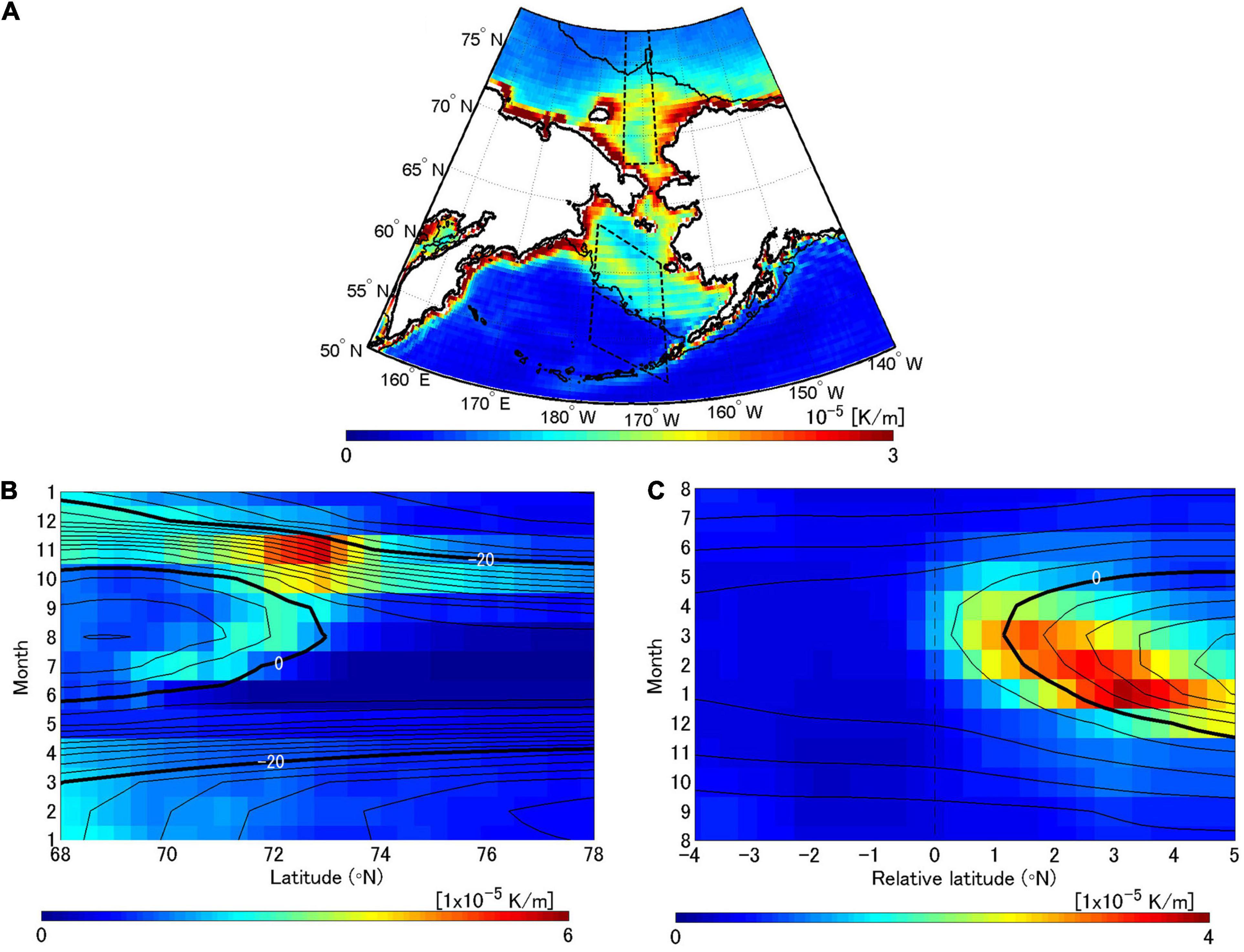
Figure 1. (A) Annual-mean climatology of the Euclidean norm of horizontal gradient of ST, and latitude-time sections of monthly climatological data of the ST horizontal gradient in (B) the Chukchi Sea and (C) the Bering Sea. Black solid lines in (A) are depth contours of 200 m. The areas enclosed with black dashed lines in (A) are the domains for (B,C). The middle dashed line near the 200-m-contour in the Bering Sea is the coordinate origin of latitude for (C). Contours in (B,C) show ST, and the intervals indicated by thin and bold contours in (B,C) are 2 and 20°C, respectively.
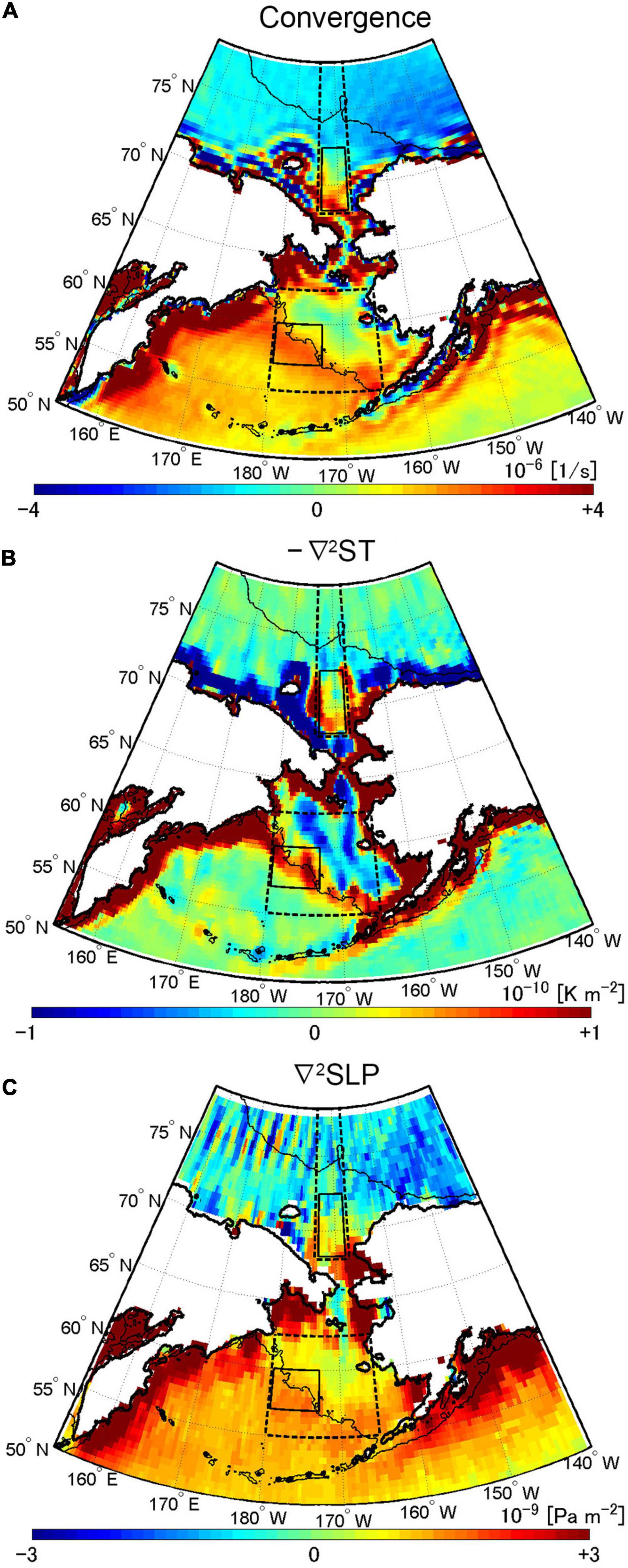
Figure 2. Annual-mean climatologies of (A) 10-m-high wind convergence, (B) the sign-reversed Laplacian of ST, and (C) the Laplacian of SLP. Black solid lines are depth contours of 200 m. Black dashed and solid boxes denote analysis areas in Figures 3, 4, respectively. A two-dimensional median filter of 5 × 5 is applied to the Laplacians of ST and SLP.
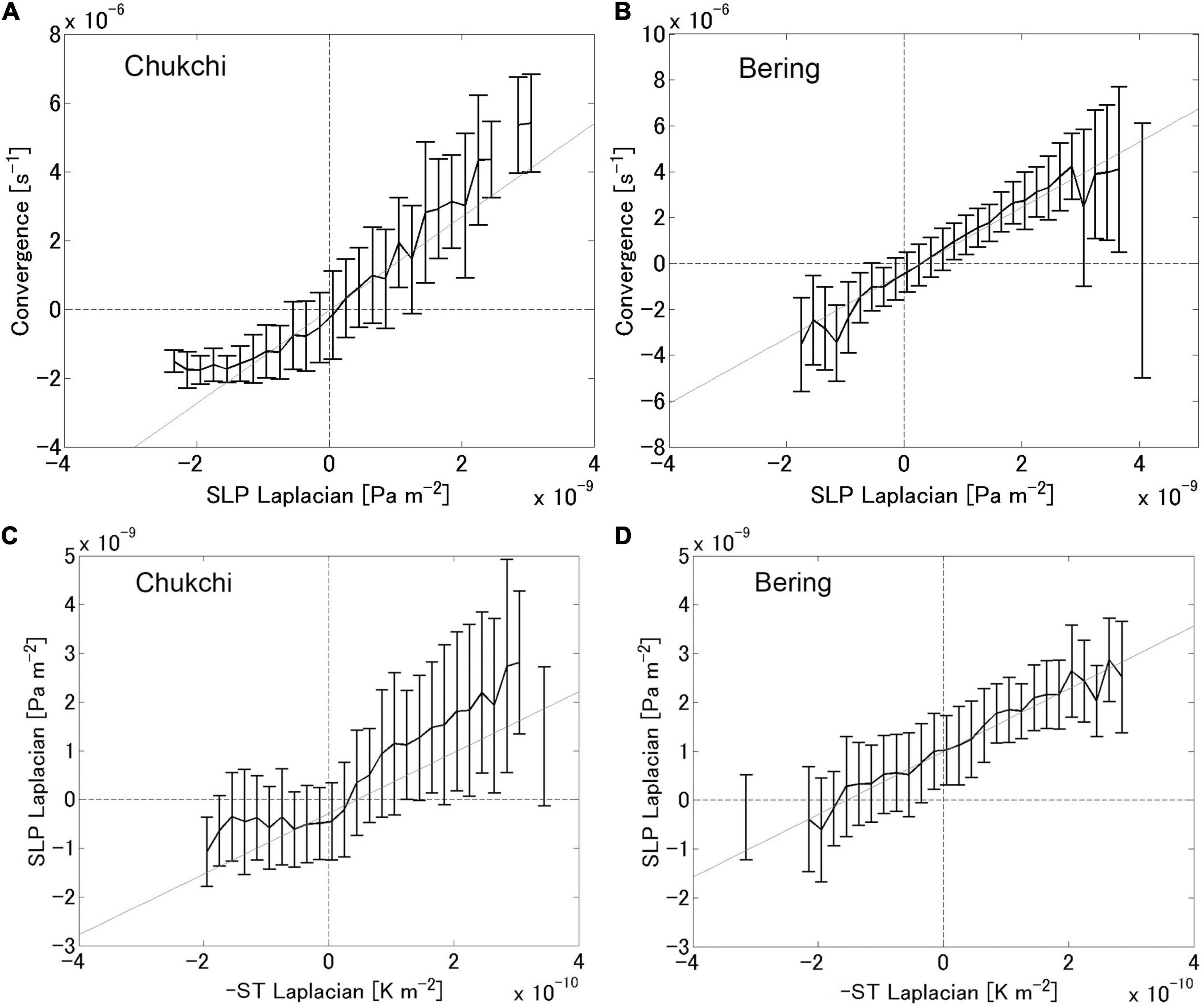
Figure 3. Annual relationships (top) between the SLP Laplacian and surface wind convergence and (bottom) between the SLP and ST Laplacians averaged over the areas defined by the black dashed boxes in Figure 2 in (A,C) the Chukchi Sea and (B,D) the Bering Sea based on monthly climatological data. Gray thin straight line is the linear regression line. Error bars denote ± 1 standard deviation. A two-dimensional median filter of 5 × 5 is applied to the Laplacians of ST and SLP.
In the Chukchi Sea, convergence of the 10-m-high wind increases in October and November, but is close to zero or even negative from January to September (Figure 4A). The seasonal cycles of ▽2SLP and ▽2ST agree well with the cycle of convergence. ST in the Chukchi Sea is highest in August, but its meridional gradient peaks in November (Figure 4C). The direction of the ST gradient vector in this region is northward in autumn. In November, sea ice is already increasing, but does not completely cover the surface, and the ST is still relatively high due to warm water coming from the Bering Sea. Conversely, ST in the region north of the Chukchi Sea drops below -20°C, which results in the largest gradient and Laplacian in November. From December, the Chukchi Sea is filled with sea ice and the ST substantially decreases.
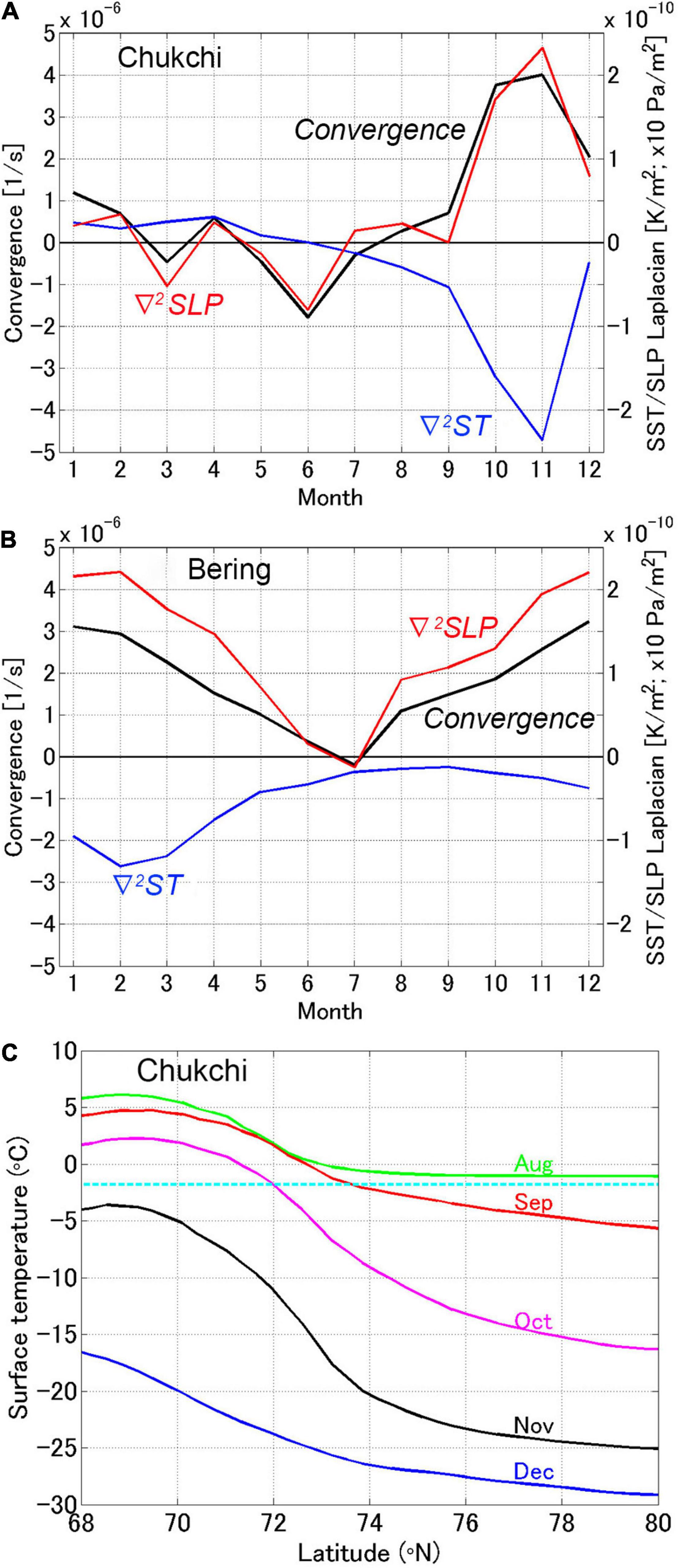
Figure 4. Monthly climatology of 10-m-high wind convergence and the Laplacians of ST and SLP averaged over the black-solid box area in Figure 2 in (A) the Chukchi Sea and (B) the Bering Sea. (C) Monthly climatological data of ST averaged between 167.5 and 174.0°W in the Chukchi Sea. Cyan dashed line represents a temperature of -1.8°C.
Regarding the atmospheric responses to ST, the vertical velocity and diabatic heating in the lower troposphere show the same seasonal cycle as the surface convergence (Figure 5). Low-level upward motion and diabatic heating develop in October and November; however, these responses are restricted to the boundary layer, unlike those in the Kuroshio and the Gulf Stream. Sasaki et al. (2012) showed that the ascending motion due to large diabatic heating extended to the upper troposphere over the Kuroshio in the East China Sea in early summer. The diabatic heating in the CFSR product consists of six components: vertical diffusion, deep convection, shallow convection, large-scale condensation, and solar and longwave radiation. The diabatic heating over the Chukchi Sea shown in Figure 5b is dominated by vertical diffusion (see Supplementary Figure 1). Large-scale condensation is the second largest component, and peaks in October (Figure 5c), which corresponds well to the cloud water mixing ratio (Figure 5e). Condensation results in low-level clouds between 950 and 800 hPa and evaporation cools the near-surface air; longwave radiation also reflects this pattern (Figure 5d). The other three components of diabatic heating are negligible. Sensible and latent heat fluxes in the Chukchi Sea are less than ± 20 W m–2 except in autumn, and both exceed 60 W m–2 in October and November (Figure 5f), leading to large near-surface diabatic heating. Basically the highly stable atmosphere suppresses forcing from the sea surface. However, in October and November, when the sea surface begins to freeze, the supply of heat and water vapor from the surface increases drastically and the heat flux gradients become large. As a result, low-level ascent and diabatic heating are organized over the Chukchi Sea, but do not penetrate the stable polar atmosphere.
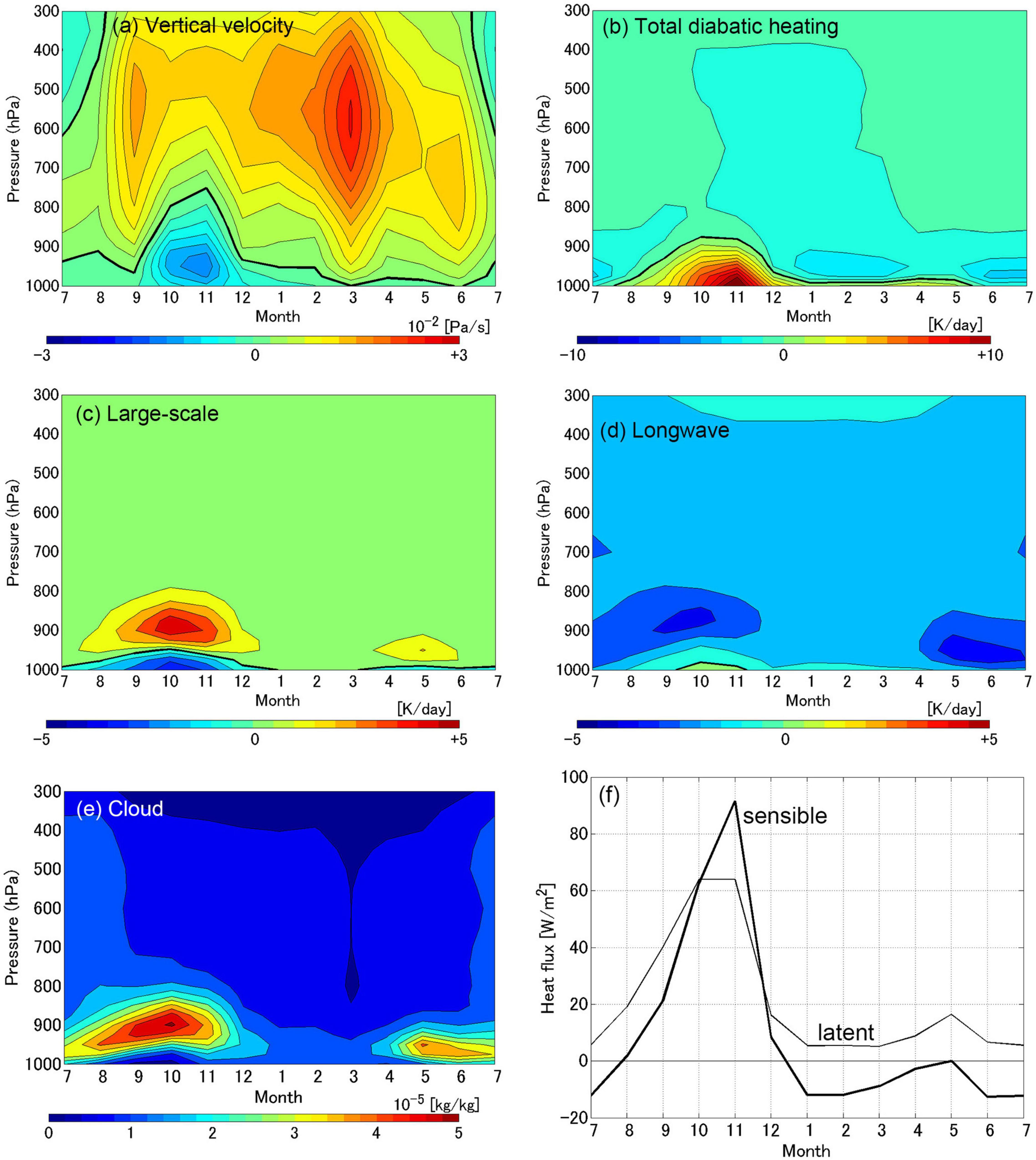
Figure 5. Seasonal variations of (a) vertical velocity, (b) total diabatic heating rate, (c) large-scale condensation component, (d) longwave radiation component, (e) cloud water mixing ratio, and (f) surface turbulent heat fluxes averaged over the area of 68.0–72.5°N, 167.5–174.0°W (black solid box in Figure 2) in the Chukchi Sea. Negative values in (a) indicate ascending motion. Black bold lines in (a–d) are zero contours.
According to the annual mean values, the surface convergence and ▽2ST are largest over the shelf break. Surface winds diverge over the continental shelf region (Figure 2A). Over the shelf break region, the convergence and ▽2SLP exhibit clear seasonality, being smaller in summer and larger in winter (Figure 4B). ▽2ST over the shelf break is negative throughout the year and especially large from January to April due to sea ice extending over the continental shelf.
The convergence-divergence pattern across the ST front corresponds to ascending motion over the shelf break and descending motion on the northern side in the lower troposphere (Figures 6a,c). This ascent-descent pattern becomes obvious in February and March (Figure 6b). The ascent that occurs in November and December extends throughout the troposphere across the shelf break, which is likely due to a synoptic-scale phenomenon rather than surface forcing. While the minimum of the climatological mean SLP is south off the Aleutian Islands, far away from the shelf break in February-March, it is located near the shelf break in November-December (see Supplementary Figure 2). This implies that the formation of the descending motion over the shelf tends to be suppressed by the ascending motion near cyclone centers in November-December. The mean meridional wind in winter is southward in the lower troposphere and northward in the middle and upper troposphere (Figure 6c). This spatial pattern of the meridional and vertical velocity implies the formation of horizontal convection over the continental shelf.
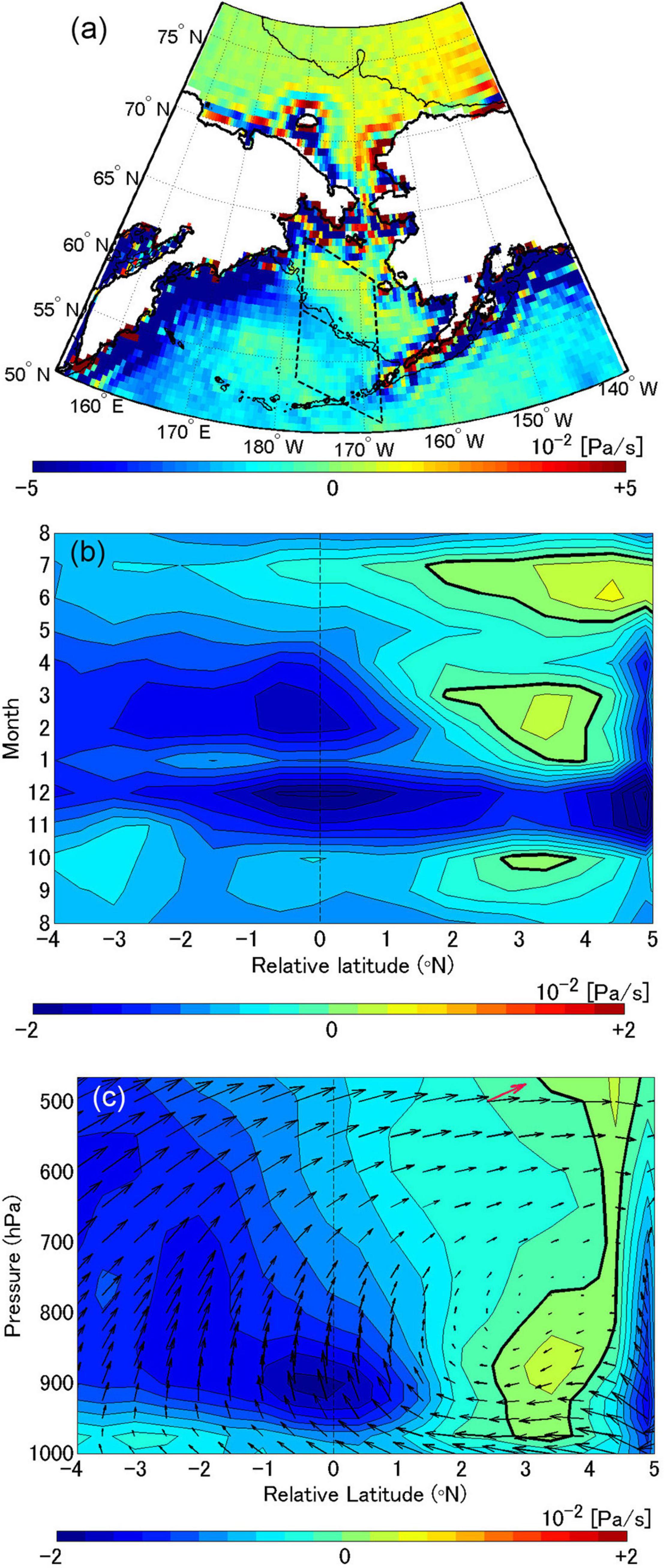
Figure 6. (a) Annual-mean climatology and (b) latitude-time section of vertical velocity between 850 and 900 hPa. (c) Latitude-altitude section of vertical velocity (color) and two-dimensional wind vector for February to March. Scaling for the arrows is given near the upper-right corner in (c) (red arrow, meridional and vertical components of 3.0 m s–1 and 1.0 × 10⁻² Pa s–1). Black bold lines in (b, c) are zero contours. The black dashed box in (a) is the average domain for (b,c).
Diabatic heating is almost confined to the boundary layer (Figure 7B) and determined by vertical diffusion (see Supplementary Figure 3), similar to the Chukchi Sea. It peaks in January and February (Figure 7A). Although the latent heat flux is largest immediately above the shelf break, the sensible heat flux and low-level diabatic heating peak over the continental shelf approximately 200 km away, where the ice concentration is approximately 15%, at the southern edge of the marginal ice zone (Figure 7E). The contours of diabatic heating in the latitude-altitude diagram slant northward, and diabatic heating at the level of 900 hPa is largest over the shelf break (Figure 7B). Large-scale condensation and the cloud water mixing ratio are noticeable between 800 hPa and 900 hPa south of the shelf break (Figures 7C,D).
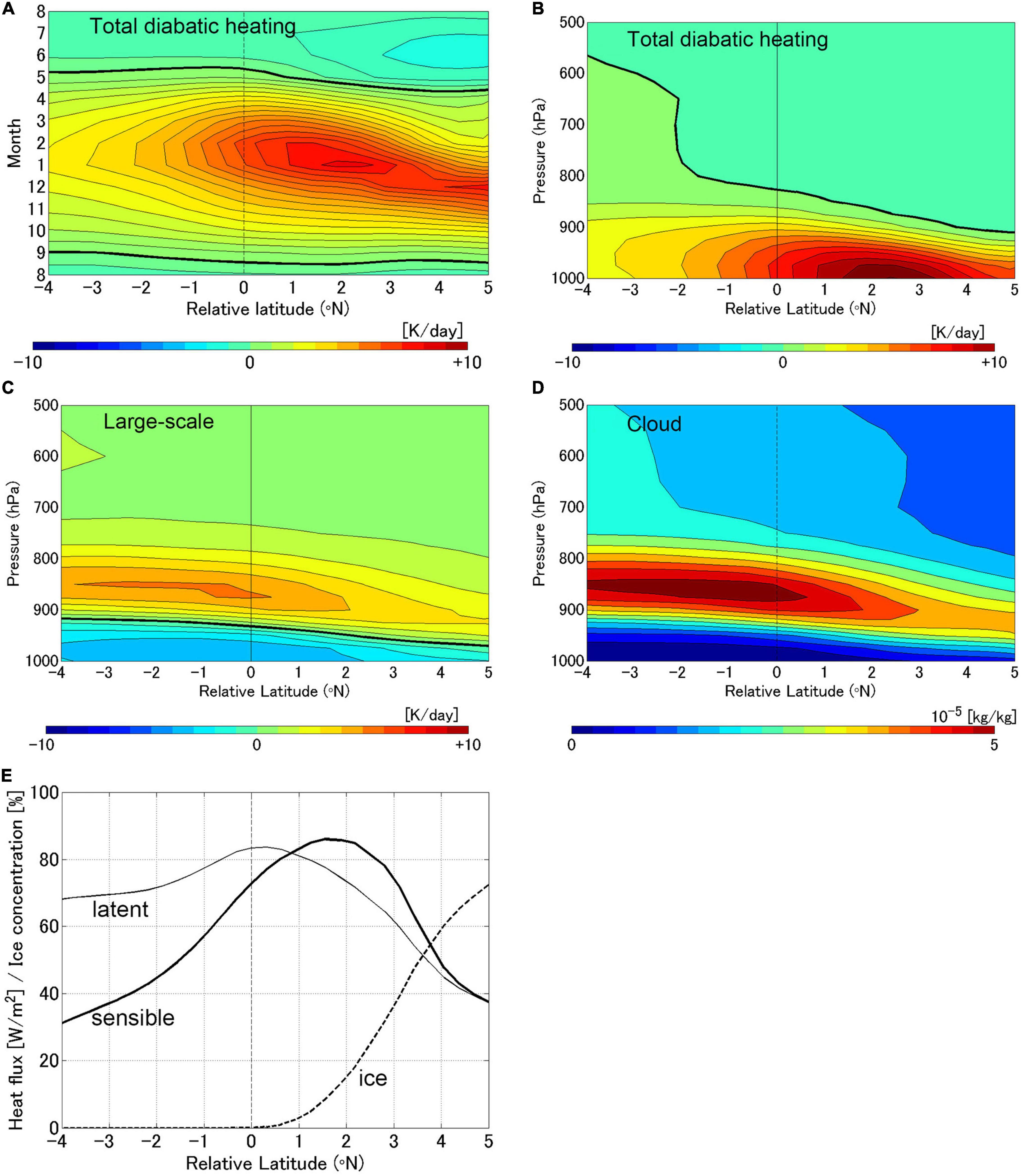
Figure 7. (A) Latitude-time section of total diabatic heating averaged between 900 and 1,000 hPa, and altitude-latitude sections of (B) total diabatic heating, (C) large-scale condensation component, and (D) cloud water mixing ratio over the Bering Sea (black dashed box in Figure 6A) for January to February. Black bold lines in (A–C) are zero contours. (E) Sensible heat flux (bold line), latent heat flux (thin line), and sea ice concentration (dashed line) for January to February.
Cloud water concentrates in the lower troposphere and exhibits a clear contrast across the shelf break in the Bering Sea. Clouds significantly affect shortwave radiation into the ocean. Figure 7D suggests that the distribution of low-level clouds reflects that of ST, whereby the horizontal gradient of cloud water below 700 hPa is large along the shelf break from winter to summer (Figure 8), although the meridional contrast vanishes in September to December (Figure 8C). The spatial distribution of downward shortwave radiation at the sea surface clearly reflects that of the low-level cloud water mixing ratio (Figures 9A,B). As solar radiation also depends on latitude, it exhibits a trough on the southern side of the shelf break in the Aleutian Basin. The precipitation rate also shows a contrast between the shallow shelf region and the deep basin, and is slightly intensified over the shelf break (Figures 9C,D).
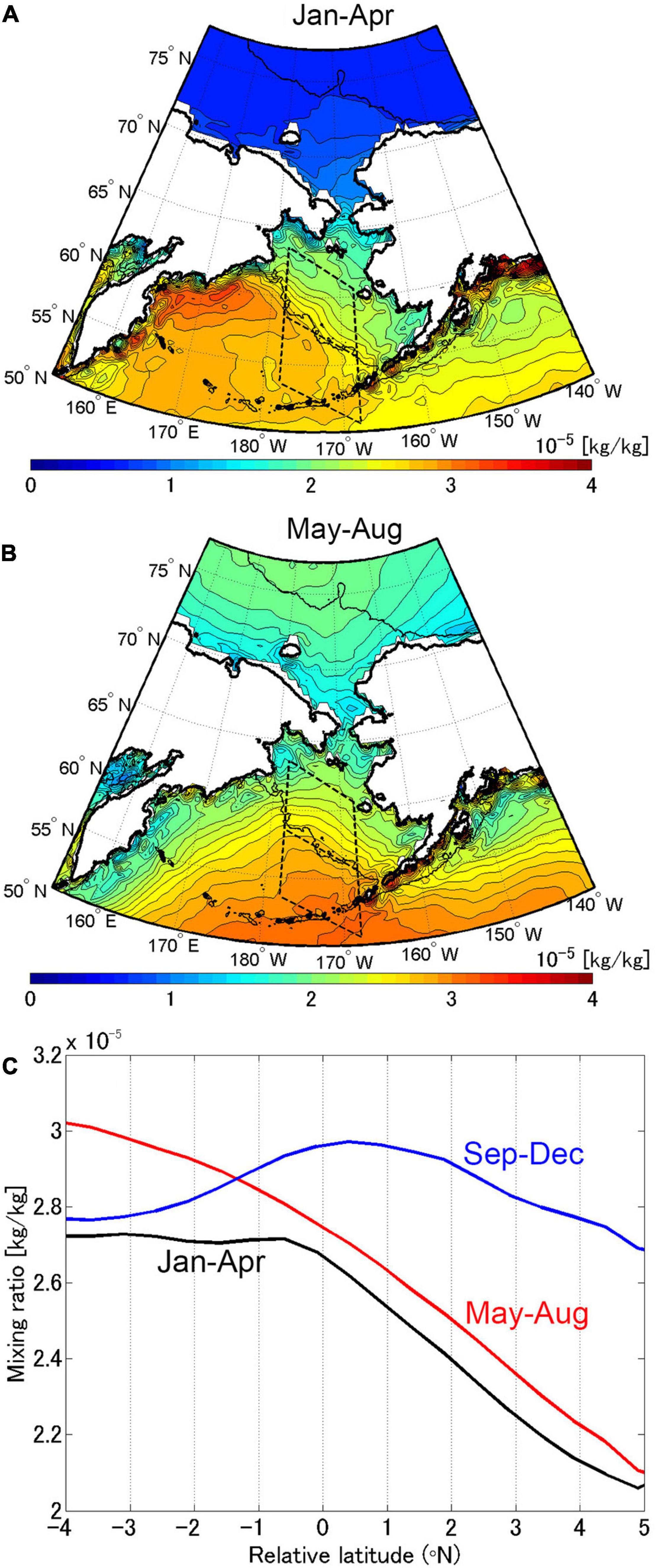
Figure 8. Climatology of the cloud water mixing ratio averaged between 700 and 1,000 hPa for (A) January to April and (B) May to August. (C) Cloud water mixing ratio from 700 to 1,000 hPa averaged over the black dashed box in (A,B) for January to April (black), May to August (red), and September to December (blue).
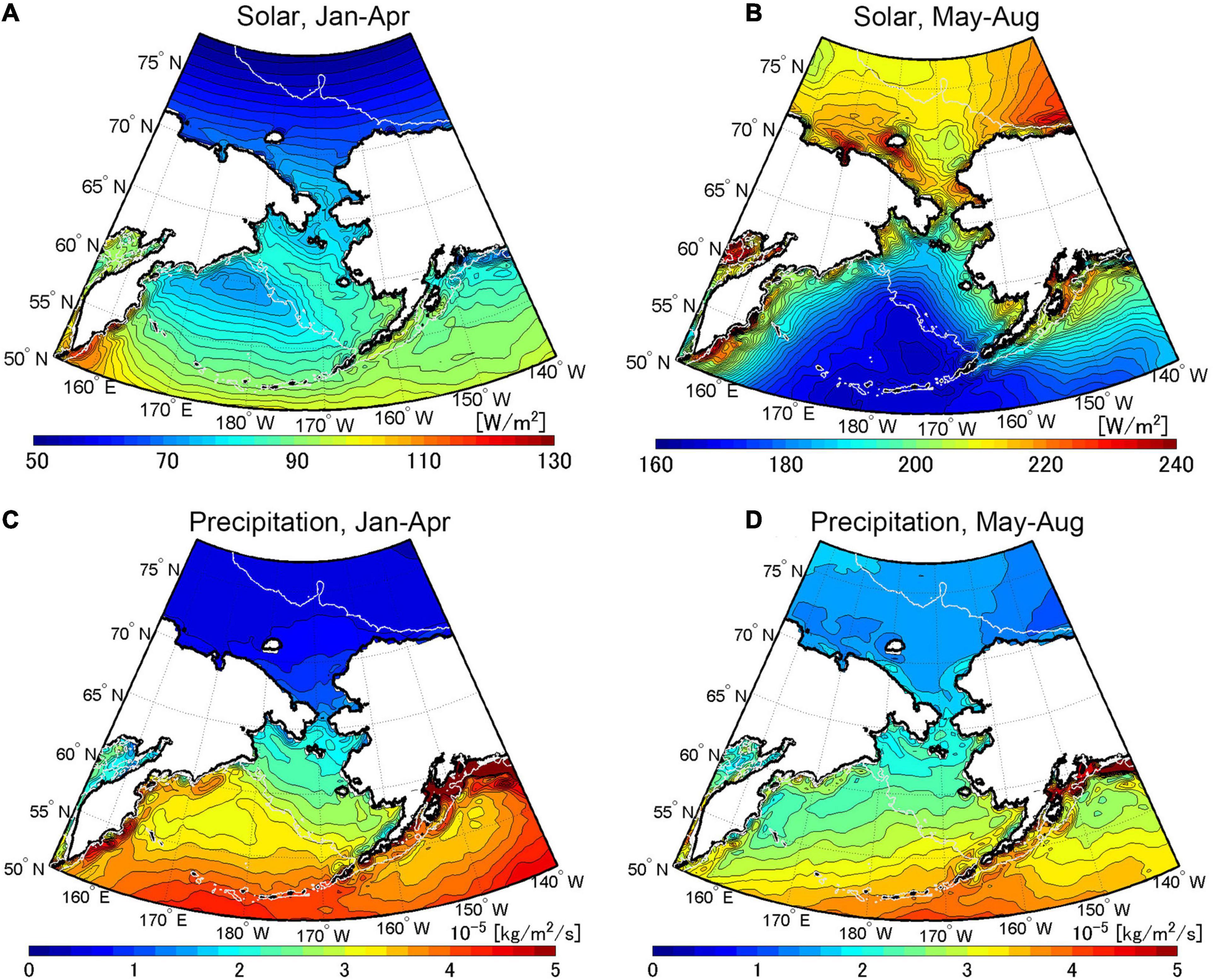
Figure 9. Climatology of (A,B) solar radiation at the sea surface and (C,D) precipitation rate for (A,C) January to April and (B,D) May to August. White lines are depth contours of 200 m.
As the wintertime oceanic mixed layer reaches the bottom in the shallow continental shelf region (Kawai et al., 2018), the mixed layer in the shelf region is cooled more than that in the deep southwestern basin. In the Bering Sea, the bottom topography regulates the upper ocean temperature and the low-level atmosphere, as Xie et al. (2002) indicated for the Yellow and East China Seas. The spatial distribution of low-level clouds that reflects the bottom topography then controls the shortwave radiation entering the ocean. Photosynthetically active radiation (PAR) is proportional to the shortwave radiation, and the characteristic pattern of incoming radiation will have an impact on the marine ecosystem in the Bering Sea.
The previous subsection described the PAM, but the VMM is also effective. The spatial distribution of high-pass-filtered ST and 10-m-high wind speed shows good correspondence, albeit with some disagreement (Figure 10). The wind speed anomalies are positive over the shelf break and the southern Chukchi Sea, where ST exhibits warm anomalies.
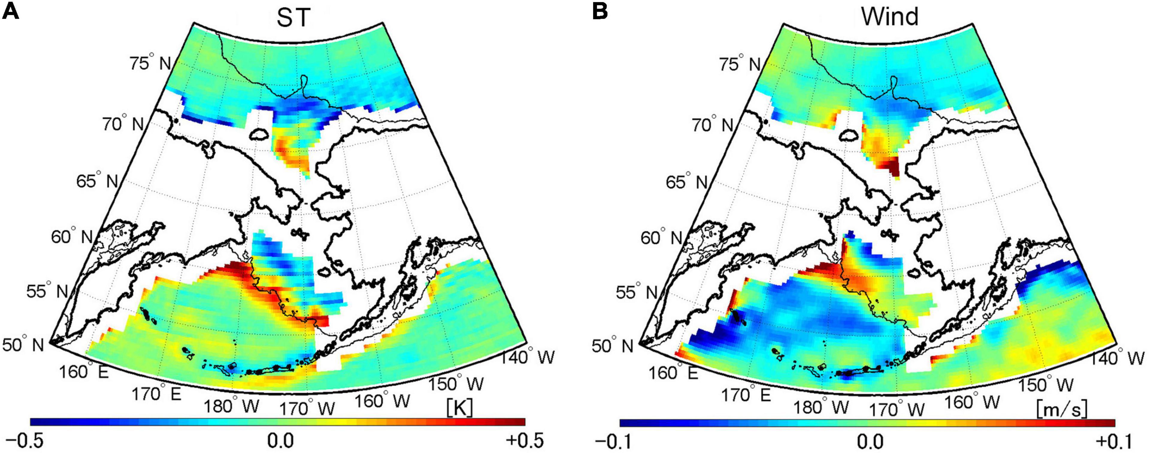
Figure 10. Annual-mean climatology of spatially high-pass-filtered (A) ST and (B) 10-m-high wind speed. The high-pass-filtered anomaly is derived as the deviation from the 5 × 5 grid mean. Black thin lines are depth contours of 200 m.
According to the diagnostics of Takatama et al. (2015), although the PAM almost completely determines the surface convergence, the surface curl is mainly accounted for by the VMM; this difference can be explained by the background wind direction with respect to the ST front. Along-front (cross-front) wind leads to wind stress curl (divergence) due to the VMM (Chelton et al., 2004), and the PAM is independent of the wind direction. Low-level geostrophic wind tends to blow parallel to the ST front in the Chukchi Sea, and perpendicular to the front in the Bering Sea (Figure 11A). A downwind ST gradient –v10⋅▽ST is observed over the continental shelf near the shelf break in the Bering Sea, and the crosswind ST gradient –v10 × ▽ST is larger than –v10⋅▽ST in the Chukchi Sea (Figures 11B,C). Thus, the contribution of downward momentum input to surface curl is expected to be relatively large in the Chukchi Sea. The convergence of downward momentum input by the VMM also reinforces surface convergence in the Bering Sea, but its relative contribution is small and the PAM dominates surface convergence.
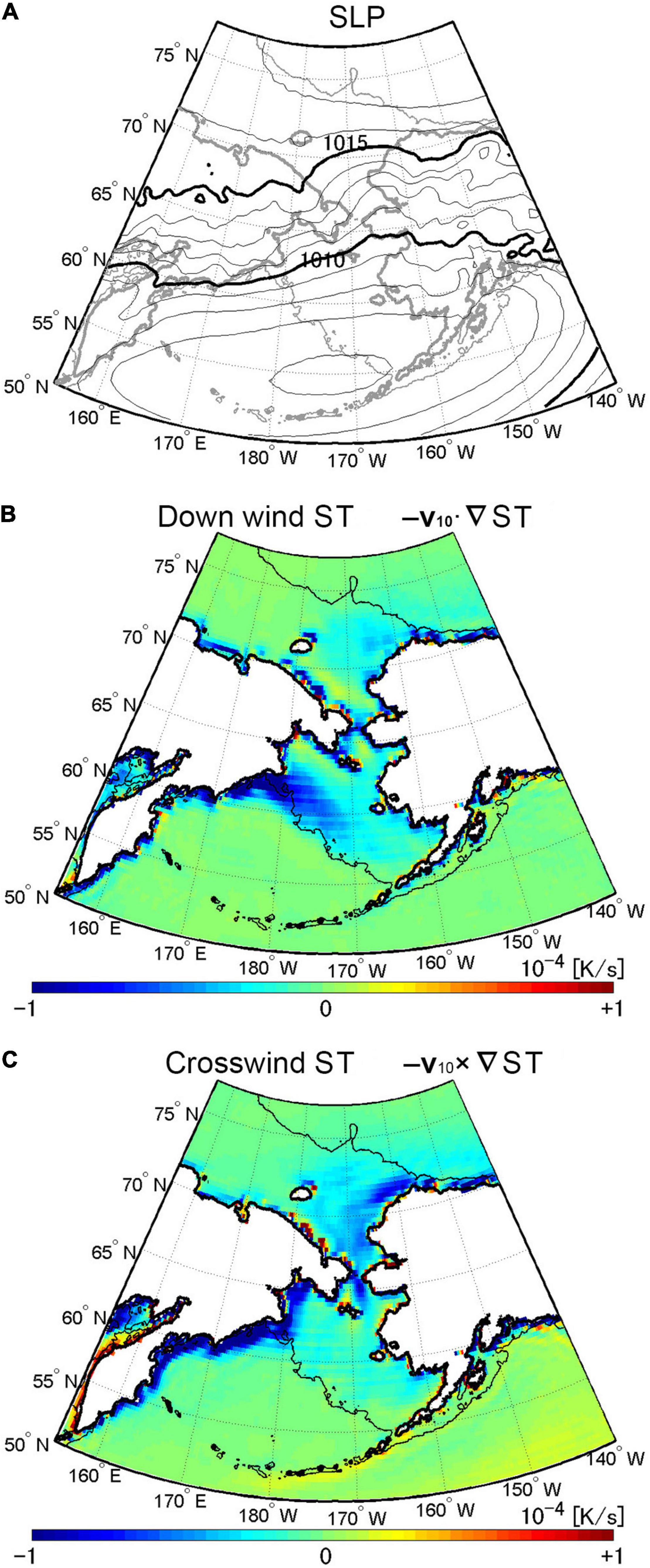
Figure 11. Annual-mean climatology of (A) SLP, (B) sign-reversed downwind ST gradient, and (C) sign-reversed crosswind ST gradient. The intervals indicated by thin and bold contours in (A) are 1 and 5 hPa, respectively.
In this study, the effect of sea ice roughness is not examined. A colder sea surface makes the atmosphere more stable and the surface wind weaker. Larger friction over sea ice has the same effect of reducing the near-surface wind speed. Hence, it is expected that the contrast in the near-surface friction across an ST front becomes much larger when sea ice exists on the cold side, which magnifies both the VMM and PAM. Sea ice roughness depends on factors such as the sea ice concentration and the thickness and age of ice; however, the effects of these factors on air-sea interactions are beyond the scope of this study.
Linear trends were calculated for the period from 1979 to 2020. The trend of ST in the Chukchi Sea is striking around 75°N in October and 72.5°N in November (Figure 12A). As a result, areas with a large ST gradient shifted northward in October and November, and the gradient around 72.5°N became larger in December due to the delay and retreat of sea ice formation (Figure 12C). In the Bering Sea, ST shows warming trends in summer and autumn, and no significant trend in winter and spring (Figure 12B). There is also no clear trend in sea ice concentration (Figure 12D). (In fact, cooling trend was seen in the northern shelf region in winter for the period until 2010, the warming in the 2010s obscured the trend.) Hereafter, the trend in the Chukchi Sea is discussed.
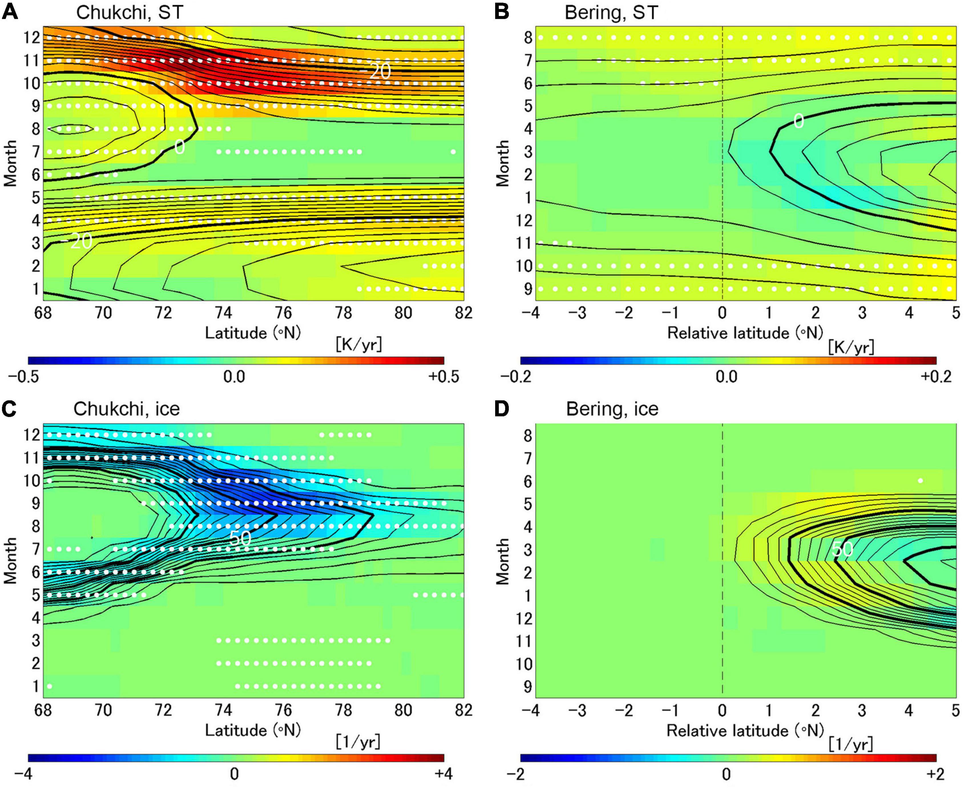
Figure 12. Latitude-time sections of (A,B) ST and (C,D) sea ice concentration trends for 1979–2020 in (A,C) the Chukchi Sea and (B,D) the Bering Sea. White dots denote statistical significance at the 95% confidence level. Contours show climatologies of (A,B) ST and (C,D) sea ice concentration. The intervals indicated by thin and bold contours are 2 and 20°C in (A,B) and 5and 25% in (C,D), respectively.
Remarkable trends of cloud water are observed in October and November (Figure 13A). Cloud water decreases near the surface but increases above 900 hPa, indicating an increase in the altitude of low-level clouds. This is consistent with the observational results of Sato et al. (2012), who showed that the base height of low-level clouds became higher as a result of the Arctic warming. A vertical velocity trend is observed near the surface in November and December, which is related to the delay of sea ice extension (Figure 13B). In October-November, the decrease of sensible heat flux in the southern Chukchi Sea (Figure 14) corresponds to the delay of freezing, suggesting that the atmospheric change led to the ocean warming. The increases of upward and downward longwave radiation at the surface balanced with each other south of 75°N. Downward shortwave radiation slightly decreased, maybe due to the change of low-level clouds. The positive trends of sensible and latent heat fluxes in 72–77°N, corresponding to the northward shift of marginal ice zone, mean that the warmed sea surface strengthened turbulent heat transfer to the atmosphere, and the warm water inflow from the Pacific Ocean (Shimada et al., 2006) would offset the surface heat loss. In the region north of 78°N, the changes of turbulent heat fluxes were negligible and the increase of downward longwave radiation was dominant. In summary, while the ocean warming increased the heat release to the atmosphere in the northern Chukchi Sea, downward radiation drove the ST rise near the polar, which is consistent with the indication of Lee et al. (2017).
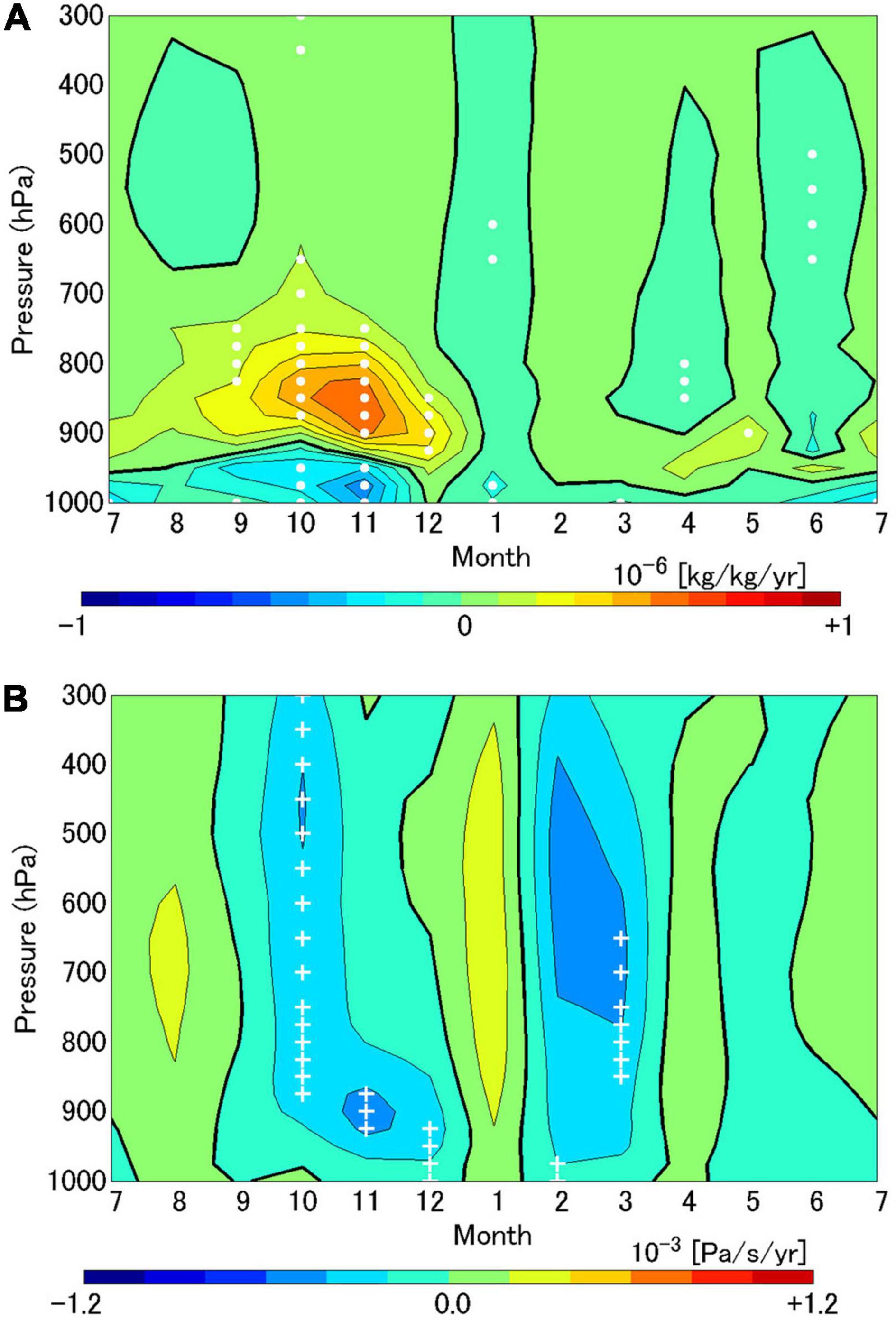
Figure 13. Trends of (A) cloud water mixing ratio and (B) vertical velocity averaged over the area of 68.0–72.5°N and 167.5–174.0°W (black solid rectangle in Figure 2A) in the Chukchi Seafor 1979–2020. Black bold lines are zero contours. White dots in (A) and pluses in (B) denote statistical significance at the 95 and 90% confidence level, respectively.
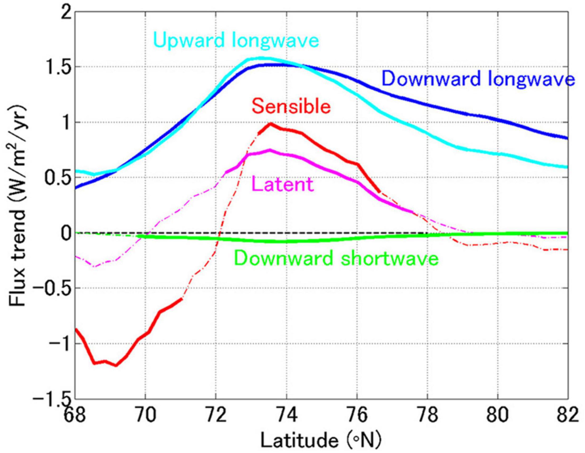
Figure 14. Trends of surface heat fluxes averaged over the area of 167.5–174.0°W in October-November for 1979–2020. Thick solid lines denote statistical significance at the 95% confidence level, and thin chained lines show no significance.
It is expected that the horizontal temperature gradient will increase substantially over the border between open water and sea ice, similar to the ST fronts related to western boundary currents in the mid latitudes; however, air-sea interaction from the viewpoint of the ST front has seldom been investigated at high latitudes. Therefore, this study examined the atmospheric responses to ST in the Chukchi and Bering Seas, where sea ice develops in the cold season, using a high-resolution atmospheric reanalysis dataset. In the Chukchi Sea, ST peaks in August, but its horizontal gradient becomes largest in November. Convergence of 10-m-high wind is also large in October and November, and approximately zero or negative from January to September. On the other hand, there is a clear contrast in ST between the continental shelf and the southwestern deep basin of the Bering Sea throughout the year, which develops in winter. The ST front shifts southward as sea ice spreads over the shelf region, and the front is located immediately above the northern flank of the shelf break in March, when the marginal ice zone extends furthest south. In both the Chukchi and Bering Seas, the spatial distribution of surface wind convergence and the Laplacians of ST and SLP agree well with each other, which demonstrates an effective PAM. The VMM is also confirmed in both seas.
Ascending motion and diabatic heating develop over the Chukchi Sea in October and November, corresponding to surface wind convergence; however, this response is confined to the lower troposphere. Diabatic heating is dominated by the vertical diffusion component. Turbulent heat fluxes at the sea surface becomes especially large in late autumn, when sea ice is increasing, resulting in the intensification of heating and low-level clouds. Ascent is also strengthened over the shelf break and a circulation pattern similar to horizontal convection appears over the shelf in the Bering Sea in late winter. Low-level clouds show a clear contrast across the shelf break in the Bering Sea, and downward solar radiation at the surface reflects the spatial pattern of the clouds. The bottom topography regulates the ST and affects clouds and incoming radiation through the ST. During 1979–2020, the Arctic Ocean including the Chukchi Sea experienced drastic warming and retreat of sea ice in autumn, although the ST exhibited no clear trends in the Bering Sea in the cold season. Over the Chukchi Sea, there was a tendency for low-level clouds to rise in October and November, which corresponded to the warming trend. This is consistent with a previous study that analyzedin situ observation data. The analysis of surface heat fluxes supported the indication of previous study that while downward longwave radiation was responsible for the ST increase near the polar, the ocean warming increased turbulent heat fluxes in the northern Chukchi Sea.
In the Chukchi and Bering Seas, the development of an ST gradient and subsequent impacts on the atmosphere are regulated by the season and bottom topography. This study only focused on the local responses; their effects on a synoptic or larger scale and their modulation under the Arctic warming should be analyzed in future research.
Publicly available datasets were analyzed in this study. This data can be found here: https://www.ncei.noaa.gov/data/climate-forecast-system/access/reanalysis/monthly-means/, https://www.ncei.noaa.gov/data/climate-forecast-system/access/operational-analysis/monthly-means-flux/, and https://www.ncei.noaa.gov/data/climate-forecast-system/access/operational-analysis/monthly-means-by-pressure/.
YK designed the study, analyzed the data, and wrote the manuscript.
This work was supported by the Japan Society for the Promotion of Science (JSPS) Grants-in-Aid for Scientific Research (B), and (C) (KAKENHI) (16H04046 and 16K05563), and also by the Ministry of Education, Culture, Sports, Science and Technology (MEXT) of Japan, Grant-in-Aid for Scientific Research on Innovative Areas (19H05700).
The author declares that the research was conducted in the absence of any commercial or financial relationships that could be construed as a potential conflict of interest.
All claims expressed in this article are solely those of the authors and do not necessarily represent those of their affiliated organizations, or those of the publisher, the editors and the reviewers. Any product that may be evaluated in this article, or claim that may be made by its manufacturer, is not guaranteed or endorsed by the publisher.
The CFSR and CFSv2 data used in this study were supplied by the NCEP.
The Supplementary Material for this article can be found online at: https://www.frontiersin.org/articles/10.3389/fmars.2021.598981/full#supplementary-material
Chelton, D. B., Schlax, M. G., Frelich, M. H., and Milliff, R. F. (2004). Satellite measurements reveal persistent small-scale features in ocean winds. Science303, 978–983. doi: 10.1126/science.1091901
Chelton, D. B., and Xie, S.-P. (2010). Coupled ocean-atmosphere interaction at oceanic mesoscales. Oceanography23, 52–69. doi: 10.5670/oceanog.2010.05
Chu, P. C. (1987). An ice breeze mechanism for an ice divergence-convergence criterion in the marginal ice zone. J. Phys. Oceanogr.17, 1627–1632. doi: 10.1175/1520-0485(1987)017<1627:aibmfa>2.0.co;2
Crawford, A. D., and Serreze, M. C. (2016). Does the summer Arctic frontal zone influence Arctic Ocean cyclone activity. J. Clim.29, 4977–4993. doi: 10.1175/JCLI-D-15-0755.1
Frankignoul, C., Sennéchael, N., Kwon, Y.-O., and Alexander, M. A. (2011). Influence of the meridional shifts of the Kuroshio and the Oyashio extensions on the atmospheric circulation. J. Clim.24, 762–777. doi: 10.1175/2010JCLI3731.1
Honda, M., Inoue, J., and Yamane, S. (2009). Influence of low Arctic sea-ice minima on anomalously cold Eurasian winters. Geophys. Res. Lett.36:L08707.
Kawai, Y., Nishikawa, H., and Oka, E. (2019). In situ evidence of low-level atmospheric responses to the Oyashio front in early spring. J. Meteor. Soc. Japan97, 423–438. doi: 10.2151/jmsj.2019-024
Kawai, Y., Osafune, S., Masuda, S., and Komuro, Y. (2018). Relations between salinity in the northwestern Bering Sea, the bering Strait throughflow and sea surface height in the Arctic Ocean. J. Oceanogr.74, 239–261. doi: 10.1007/s10872-017-0453-x
Lee, S., Gong, T., Feldstein, S. B., Screen, J. A., and Simmonds, I. (2017). Revisiting the cause of the 1989-2009 Arctic surface warming using the surface energy budget: downward infrared radiation dominates the surface fluxes. Geophys. Res. Lett.44, 10654–10661. doi: 10.1002/2017GL075375
Luo, B., Luo, D., Wu, L., Zhong, L., and Simmonds, I. (2017). Atmospheric circulation patterns which promote winter Arctic sea ice decline. Environ. Res. Lett.12:054017. doi: 10.1088/1748-9326/aa69d0
Luo, B., Wu, L., Luo, D., Dai, A., and Simmonds, I. (2019). The winter midlatitude-Arctic interaction: effects of North Atlantic SST and high-latitude blocking on Arctic sea ice and Eurasian cooling. Clim. Dyn.52, 2981–3004. doi: 10.1007/s00382-018-4301-5
Luo, D., Chen, X., Overland, J., Simmonds, I., Wu, Y., and Zhang, P. (2019). Weakened potential vorticity barrier linked to recent winter Arctic sea ice loss and midlatitude cold extremes. J. Clim.32, 4235–4261. doi: 10.1175/JCLI-D-18-0449.1
Masunaga, R., Nakamura, H., Miyasaka, T., Nishii, K., and Tanimoto, Y. (2015). Separation of climatological imprints of the Kuroshio extension and Oyashio fronts on the wintertime atmospheric boundary layer: their sensitivity to SST resolution prescribed for atmospheric reanalysis. J. Clim.28, 1764–1787. doi: 10.1175/JCLI-D-14-00314.1
McCusker, K. E., Fyfe, J. C., and Sigmond, M. (2016). Twenty-five winters of unexpected Eurasian cooling unlikely due to Arctic sea-ice loss. Nat. Geosci.9, 838–842. doi: 10.1038/ngeo2820
Minobe, S., Kuwano-Yoshida, A., Komori, N., Xie, S. –P., and Small, R. J. (2008). Influence of the gulf stream on the troposphere. Nature452, 206–209. doi: 10.1038/nature06690
Mori, M., Kosaka, Y., Watanabe, M., Nakamura, H., and Kimoto, M. (2019). A reconciled estimate of the influence of Arctic sea-ice on recent Eurasian cooling. Nat. Clim. Change9, 123–129. doi: 10.1038/s41558-018-0379-3
Rudeva, I., and Simmonds, I. (2021). Midlatitude winter extreme temperature events and connections with anomalies in the Arctic and tropics. J. Clim.34, 1–47. doi: 10.1175/JCLI-D-20-0371.1
Saha, S., Moorthi, S., Pan, H. L., Wu, X. R., Wang, J. D., Nadiga, S., et al. (2010). The NCEP climate forecast system reanalysis. Bull. Amer. Meteor. Soc.91, 1015–1057. doi: 10.1175/2010BAMS3001.1
Saha, S., Moorthi, S., Wu, W., Wang, J., Nadiga, S., Tripp, P., et al. (2014). The NCEP climate forecast system version 2. J. Clim.27, 2185–2208. doi: 10.1175/JCLI-D-12.00823.1
Sasaki, Y. N., Minobe, S., Asai, T., and Inatsu, M. (2012). Influence of the Kuroshio in the East China Sea on the early summer (Baiu) rain. J. Clim.25, 6627–6645. doi: 10.1175/JCLI-D-11-00727.1
Sato, K., Inoue, J., Kodama, Y., and Overland, J. E. (2012). Impact of Arctic sea-ice retreat on the recent change in cloud-base height during autumn. Geophys. Res. Lett.39:L10503. doi: 10.1029/2012GL051850
Sato, K., Inoue, J., Simmonds, I., and Rudeva, I. (2021). Antarctic Peninsula warm winters influenced by Tasman Sea temperatures. Nat. Commun.12:1497. doi: 10.1038/s41467-021-21773-5
Sato, K., Inoue, J., and Watanabe, M. (2014). Influence of the gulf stream on the Barents sea ice retreat and Eurasian coldness during early winter. Environ. Res. Lett.9:084009. doi: 10.1088/1748-9326/9/8/084009
Seo, H., and Yang, J. (2013). Dynamical response of the Arctic boundary layer process to uncertainties in sea-ice concentration. J. Geophys. Res. Atmos.118, 12383–12402. doi: 10.1002/2013JD020312
Shimada, K., Kamoshida, T., Itoh, M., Nishino, S., Carmack, E., McLaughlin, F., et al. (2006). Pacifici Ocean inflow: influence on catastrophic reduction of sea ice cover in the Arctic Ocean. Geophys. Res. Lett.33:L08605. doi: 10.1029/2005GL025624
Shimada, T., and Minobe, S. (2011). Global analysis of the pressure adjustment mechanism over sea surface temperature fronts using AIRS/Aqua data. Geophys. Res. Lett.38:L06704. doi: 10.1029/2010GL046625
Tachibana, Y., Komatsu, K. K., Alexeev, V. A., Cai, L., and Ando, Y. (2019). Warm hole in Pacific Arctic sea ice cover forced mid-latitude Northern Hemisphere cooling during winter 2017-18. Sci. Rep.9:5567. doi: 10.1038/s41598-019-41682-4
Taguchi, B., Nakamura, H., Nonaka, M., Komori, N., Kuwano-Yoshida, A., Takaya, K., et al. (2012). Seasonal evolutions of atmospheric response to decadal SST anomalies in the North Pacific subarctic frontal zone: observations and a coupled model simulation. J. Clim.25, 111–139. doi: 10.1175/JCLI-D-11-00046.1
Takatama, K., Minobe, S., Inatsu, M., and Small, R. J. (2015). Diagnostics for near-surface wind response to the gulf stream in a regional atmospheric model. J. Clim.28, 238–255. doi: 10.1175/JCLI-D-13-00668.1
Tokinaga, H., Tanimoto, Y., Xie, S.-P., Sampe, T., Tomita, H., and Ichikawa, H. (2009). Ocean frontal effects on the vertical development of clouds over the western north Pacific: in situ and satellite observations. J. Clim.22, 4241–4260. doi: 10.1175/2009JCLI2763.1
Vaughan, D. G., Comiso, J. C., Allison, I., Carrasco, J., Kaser, G., Kwok, R., et al. (2013). “Observations: cryosphere,” in Climate Change 2013: The Physics Science Basis. Contribution of Working Group I to the Fifth Assessment Report of the Intergovernmental Panel on Climate Change, eds T. F.Stocker et al. (Cambridge, NY: Cambridge University Press).
Wallace, J. M., Mitchell, T. P., and Deser, C. (1989). The influence of sea-surface temperature on surface wind in the eastern equatorial Pacific: seasonal and interannual variability. J. Clim.2, 1492–1499. doi: 10.1175/1520-0442(1989)002<1492:tiosst>2.0.co;2
Xie, S.-P., Hafner, J., Tanimoto, Y., Liu, W. T., Tokinaga, H., and Xu, H. (2002). Bathymetric effect on the winter sea surface temperature and climate of the Yellow and East China Seas. Geophys. Res. Lett.29:L2228. doi: 10.1029/2002GL015884
Keywords: Bering Sea, Chukchi Sea, air-sea interaction, pressure adjustment, vertical mixing, sea surface temperature, sea ice, Climate Forecast System Reanalysis
Citation: Kawai Y (2021) Low-Level Atmospheric Responses to the Sea Surface Temperature Fronts in the Chukchi and Bering Seas. Front. Mar. Sci. 8:598981. doi: 10.3389/fmars.2021.598981
Received: 26 August 2020; Accepted: 01 July 2021;
Published: 26 July 2021.
Edited by:
Petra Heil, Australian Antarctic Division, AustraliaReviewed by:
Katherine Hedstrom, University of Alaska Fairbanks, United StatesCopyright © 2021 Kawai. This is an open-access article distributed under the terms of the Creative Commons Attribution License (CC BY). The use, distribution or reproduction in other forums is permitted, provided the original author(s) and the copyright owner(s) are credited and that the original publication in this journal is cited, in accordance with accepted academic practice. No use, distribution or reproduction is permitted which does not comply with these terms.
*Correspondence: Yoshimi Kawai, eWthd2FpQGphbXN0ZWMuZ28uanA=
Disclaimer: All claims expressed in this article are solely those of the authors and do not necessarily represent those of their affiliated organizations, or those of the publisher, the editors and the reviewers. Any product that may be evaluated in this article or claim that may be made by its manufacturer is not guaranteed or endorsed by the publisher.
Research integrity at Frontiers
Learn more about the work of our research integrity team to safeguard the quality of each article we publish.