Detection of Coral Reef Bleaching Based on Sentinel-2 Multi-Temporal Imagery: Simulation and Case Study

Sentinel-2 mission has been shown to have promising applications in coral reef remote sensing because of its superior properties. It has a 5-day revisit time, spatial resolution of 10 m, free data, etc. In this study, Sentinel-2 imagery was investigated for bleaching detection through simulations and a case study over the Lizard Island, Australia. The spectral and image simulations based on the semianalytical (SA) model and the sensor spectral response function, respectively, confirmed that coral bleaching cannot be detected only using one image, and the change analysis was proposed for detection because there will be a featured change signal for bleached corals. Band 2 of Sentinel-2 is superior to its other bands for the overall consideration of signal attenuation and spatial resolution. However, the detection capability of Sentinel-2 is still limited by the water depth. With rapid signal attenuation due to the water absorption effect, the applicable water depth for bleaching detection was recommended to be less than 10 m. The change analysis was conducted using two methods: one radiometric normalization with pseudo invariant features (PIFs) and the other with multi-temporal depth invariant indices (DII). The former performed better than the latter in terms of classification. The bleached corals maps obtained using the PIFs and DII approaches had an overall accuracy of 88.9 and 57.1%, respectively. Compared with the change analysis based on two dated images, the use of a third image that recorded the spectral signals of recovered corals or corals overgrown by algae after bleaching significantly improved the detection accuracy. All the preliminary results of this article will aid in the future studies on coral bleaching detection based on remote sensing.

Introduction

Coral reefs have long supported healthy coasts and thousands of businesses. However, global warming is emerging as a major threat to coral reefs. It has resulted in coral bleaching, i.e., stressed corals expel their symbiotic algae, increasing the possibility of subsequent coral morbidity and mortality. This trend has been increasing in frequency and severity all over the world. Many studies have documented regional or global coral bleaching patterns and impacts using field observations data or reef environmental conditions retrieving from satellite data over the past several decades (Barkley et al., 2018; Hughes et al., 2018a). These studies emphasize the understanding of the relationship between environmental factors and coral bleaching. There is an urgent need for better mapping of coral bleaching in a time- and cost-effective way.

Thus far, remote sensing technologies have been verified as useful tools to monitor coral reefs (Mumby et al., 1999; Hedley et al., 2016). Remote sensing data with high spatial and spectral resolution will aid in mapping benthic habitats in considerable detail with higher accuracy (Hochberg and Atkinson, 2003; Kutser et al., 2020). In the last 40 years, the satellite instruments used for coral reef applications have significantly developed over generations. In the first stage, many studies on benthic classification have shown that Landsat and SPOT are suitable for mapping geomorphological zones with low to moderate complexity (Lyzenga, 1981; Leon and Woodroffe, 2011; Phinn et al., 2012; Roelfsema et al., 2013; Xu et al., 2016). It is generally believed that hyperspectral data can be used to diagnose spectral characteristics over different benthic classes. However, previous studies have primarily focused on very high spatial resolution multispectral data because of the heterogeneity of coral reefs at scales of few meters or less, such as images from some commercial instruments of Quickbird and WorldView, in spite of their expensive cost. Coral reef remote sensing is expected to improve with the advent of the Copernicus Sentinel-2 mission. It comprises a constellation of two polar-orbiting satellites and offers a new paradigm that is significantly different from previous instruments. It combines several superior features for coral reef monitoring. Similar to Landsat 8, it has a blue band that might improve atmospheric correction and enable the imaging of shallow waters in coral reefs, but with a finer spatial resolution of 10 m. More importantly, it has a short coverage period and revisits coastal zones every five days, thus facilitating the use of time series or change detection methods that are extremely important in some reef applications, such as coral reef bleaching detection.

It was considered that extracting information on bleached corals using satellite imagery is infeasible or extremely difficult (Elvidge et al., 2004). This was because bleached corals have similar spectral values as sand, and their reflectance is similar to corals covered by algae or live corals because of the mixed pixels effect. It is difficult to capture bleaching through satellite images as this phenomenon generally occurs over weeks. On the most resilient reefs, bleached corals can regain their color within a period of weeks to months once the water temperature returns to normal (Douglas, 2003). However, obtaining remote sensing data with rapid revisit times will provide a chance to capture the change signals that are exclusively related to bleached corals based on the change analysis.

Thus far, although some studies have documented the improved ability of Sentinel-2 for reef benthic classification and coral bleaching detection (Hedley et al., 2012, 2018), this data has not been effectively used for bleaching detection. Moreover, studies that performed bleaching detection using one image have considerable uncertainty, and the results are not satisfactorily accurate because of the similar and indistinguishable spectral signals of different reef substrates (Andréfouët et al., 2002; Philipson and Lindell, 2003; Clark et al., 2010). In addition, the overall conclusion from the studies on change analysis implies that bleaching detection at regional to global scales is still challenging (Elvidge et al., 2004; Yamano and Tamura, 2004). These limitations are attributed to the insufficient spatial resolutions that may cause problems of mixed pixels, as well as the methods used for precise cross-image radiometric alignment and change signal extraction.

The present study has two objectives: (1) To evaluate the effectiveness of Sentinel-2 images in detecting coral bleaching under different conditions such as bleaching severity and water depth; and (2) to compare different change analysis methods for bleaching detection through a case study at the Lizard Island, Australia. Then, a method is proposed after an accuracy assessment.

Materials and Methods

Study Site

The present study was conducted at the Lizard Island group, which is a part of the Northern Great Barrier Reef, located 241 km north of Cairns and 92 km north east off the coast from Cooktown, Australia (Figure 1). It is a typical “shallow offshore reef” that is visible in optical remote sensing imagery to a depth of 20 m Lowest Astronomical Tide (LAT) (Roelfsema et al., 2018). The tidal range at Lizard Island is about 3 m (Daly, 2005; Hamylton et al., 2014). Many studies have documented the record-breaking sea temperatures for 2014–2017 at different levels, which have triggered mass coral bleaching in the Caribbean, Indian, and Pacific oceans and the Great Barrier Reef (Hughes et al., 2017). The site was chosen as the case study because of the obvious coral bleaching observed here. It also represents the typical coral conditions of Australia. There is existing field data on its bleaching (Great Barrier Reef Marine Park Authority, 2017; Hughes et al., 2017). For example, the Great Barrier Reef Marine Park Authority reported that the Great Barrier Reef recorded its hottest-ever average sea surface temperatures for February, March, April, May, and June in 2016 (Great Barrier Reef Marine Park Authority, 2017). This had a severe bleaching impact on the majority of the reef north of Cairns; more than 60% of the corals were bleached in March 2016. Then, a high coral mortality between the tip of Cape York and just north of the Lizard Island was observed in June 2016 because of severe bleaching.

FIGURE 1

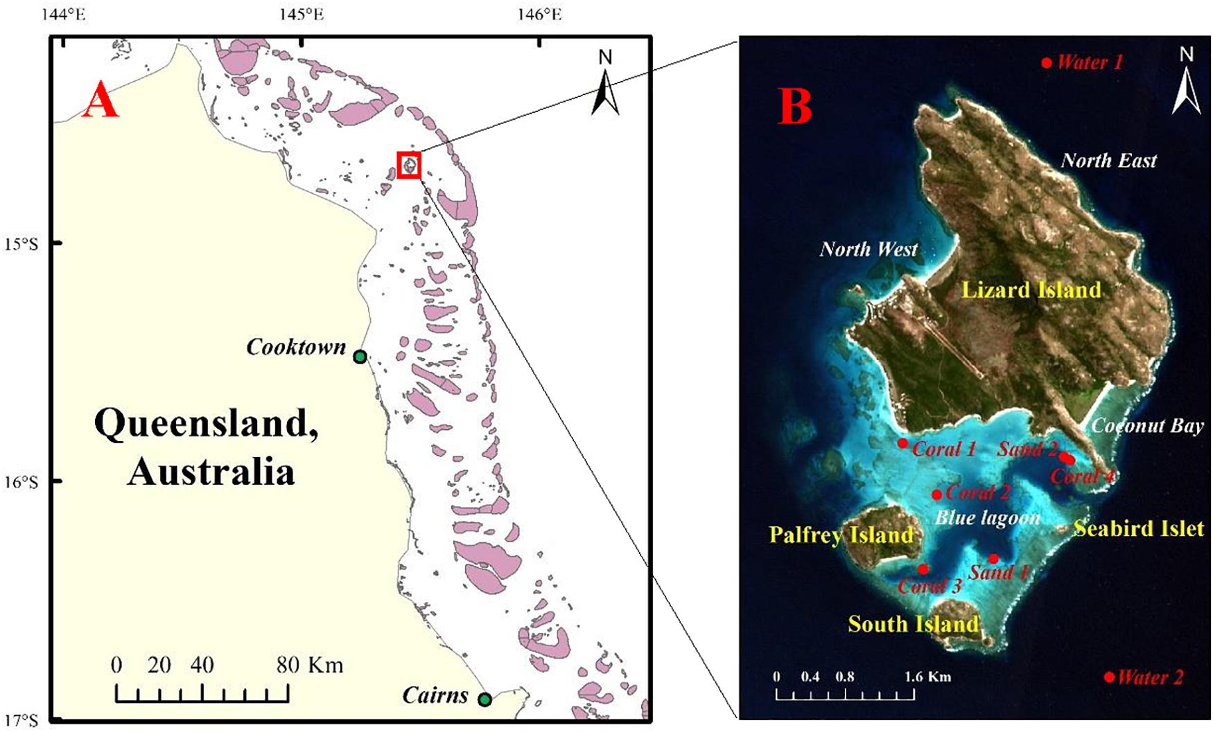
Figure 1. Study sites in this article. (A) Map shows the general position of the Lizard Island, (B) RGB composites of bands 4, 3, and 2 of Sentinel-2A image over the Lizard Island. The red points of coral, sand, and deep water are part of ground truth data and will be used for the spectral analysis and classification training.

Data Collection

Satellite Images

A total of 7 MultiSpectral Instrument (MSI) images from Sentinel-2A mission were downloaded and selected for mapping bleached corals over the Lizard Island. Considerable efforts were made to choose images with little to no cloud cover over the main island areas. The main details of these selected images are provided in Table 1. All images are Level-1C products obtained using a digital elevation model (DEM) to project the image on cartographic coordinates. The per-pixel radiometric measurements are provided in top of atmosphere reflectance.

TABLE 1

Table 1. Sentinel-2A MSI images used to analyze coral bleaching over the Lizard Island.

Ground Truth Data

The ground truth data for the Lizard Island were obtained in several ways. The Australian Research Council (ARC) Centre of Excellence performed comprehensive surveys in March 2016, providing a rapid reef-wide assessment of the spatial extent of shallow coral bleaching within the Great Barrier Reef Marine Park (Great Barrier Reef Marine Park Authority, 2017; Hughes et al., 2017, 2018b). The coral bleaching score was recorded as a categorical variable. This survey data contained four records on coral bleaching in the Lizard Island (North East, North West, Coconut Bay and Lagoon in Figure 1B). Each point was assigned by visual assessment to one of five categories of bleaching severity: (0) less than 1% of corals bleached, (1) 1–10%, (2) 10–30%, (3) 30–60%, and (4) more than 60% of corals bleached. Underwater surveys of the coral bleaching were conducted at the same time using five 10 × 1 m belt transects placed on the reef crest at a depth of 2 m at the site of North East. In the studies of Wismer et al. (2019) and Tebbett et al. (2019), coral bleaching was documented on another 19 sites on the reef crest at 0–4 m below chart-datum, and they also noted a significant decrease in live coral cover over Lizard Island. In addition, the images captured in March 2016 around the Palfrey island (14°41′46″ S, 145°27′03″ E) by Underwater Earth and the ocean agency for the documentary film “Chasing Coral” also showed coral bleaching (Coral 3 in Figure 1B). For further comparison, a substantial habitat map derived from a photo-transect survey field data in 2011 and 2012 was used as reference data for bleaching detection (Roelfsema et al., 2014). These field data were used to calibrate or validate the bleaching maps produced in this study.

Methods

General Sheme

In previous studies, Sentinel-2 was verified to have improved ability in terms of its spatial resolution, instrument noise, usable acquisition rate, large coverage, etc. (Hedley et al., 2012, 2018). Therefore, the first part of this will follow-up on these analyses based on spectral and image simulation using a semianalytical (SA) model (Lee et al., 1998, 1999) and the Sentinel-2 band relative spectral response (RSR) functions. Spectral separability of different substrates or bleached corals at different severity, as well as the water absorption effects at different water depths will be discussed based on the simulation. The results of simulation will also guide the band selection for subsequent change analysis. To further assess the sensitivity of Sentinel-2A mission to reef signals, the environmental noise equivalent delta reflectance (NEΔR_E) (Wettle et al., 2004; Brando et al., 2009) was calculated based on the image taken in November 2015 and compared with signal difference of bleached and healthy corals at different water depths.

It is widely believed that coral bleaching can be a short-lived phenomenon, where corals can recover after being bleached or they might be overgrown with algae in several weeks. Consequently, the signals received by the sensors generally exhibit a synchronous increase when the coral bleaches and there is a decrease after bleaching. This provides a basis for bleaching detection using the change analysis. However, in most cases, the subtle bleaching change signals collected by the sensors will be interfered by non-scene-dependent signals caused by atmospheric degradation, water attenuation, radiometric differences in multi-temporal imagery, etc. Therefore, it is necessary to constrain the interference to make the desired change signals more explicit.

To obtain more accurate results, some image preprocessing is required before the change analysis. This includes atmospheric correction, geo-registration, deglint, and masking. For the change analysis, two methods were compared for a better bleaching mapping. The first employed a scene-to-scene radiometric normalization technique based on pseudo invariant features (PIFs) corresponding to optically bright (shallow sand) and dark (deep waters) targets (Schott et al., 1988; Elvidge et al., 2004). The image obtained on August 30, 2016 with few clouds was considered as the baseline data. The other images were normalized to this baseline image. The representative areas of shallow sand and deep water were delineated in advance. Then, multi-temporal images of normalized signals on different dates were generated. Theoretically, for normalized images, the pixel value of bleached coral generally shows an upward initially, and then a downward trend. Therefore, if a pixel resembles that of sample bleached corals in the time series classification, it will be identified as a bleached coral. To achieve a higher accuracy based on the limited sample points, the support vector machine (SVM) classifier will be applied to the processed time series images because of its superior generalization properties and high performance (Gapper et al., 2019; Xu H. et al., 2019). A radial basis function kernel method was used for each classification based on the optimal accuracy and generalization criteria. The class for each pixel was determined by thresholding the posterior probability at 50%. The pixels that were classified as similar objects to the sample points in all three SVM applications (before, during, and after bleaching) will be identified as bleached corals. The field points contaminated by cloud or white cap and the four coral points in Figure 1 used for classifier training were excluded from the 19 ground truth points of the bleached corals. Then, 13 points were remained for validating the bleached maps, and 50 sand/rubble points were randomly selected by visual interpretation (Figure 2). The 50 sand/rubble points were set as unclassified types other than the bleached corals since sand/rubble was comparatively easy to discern.

FIGURE 2

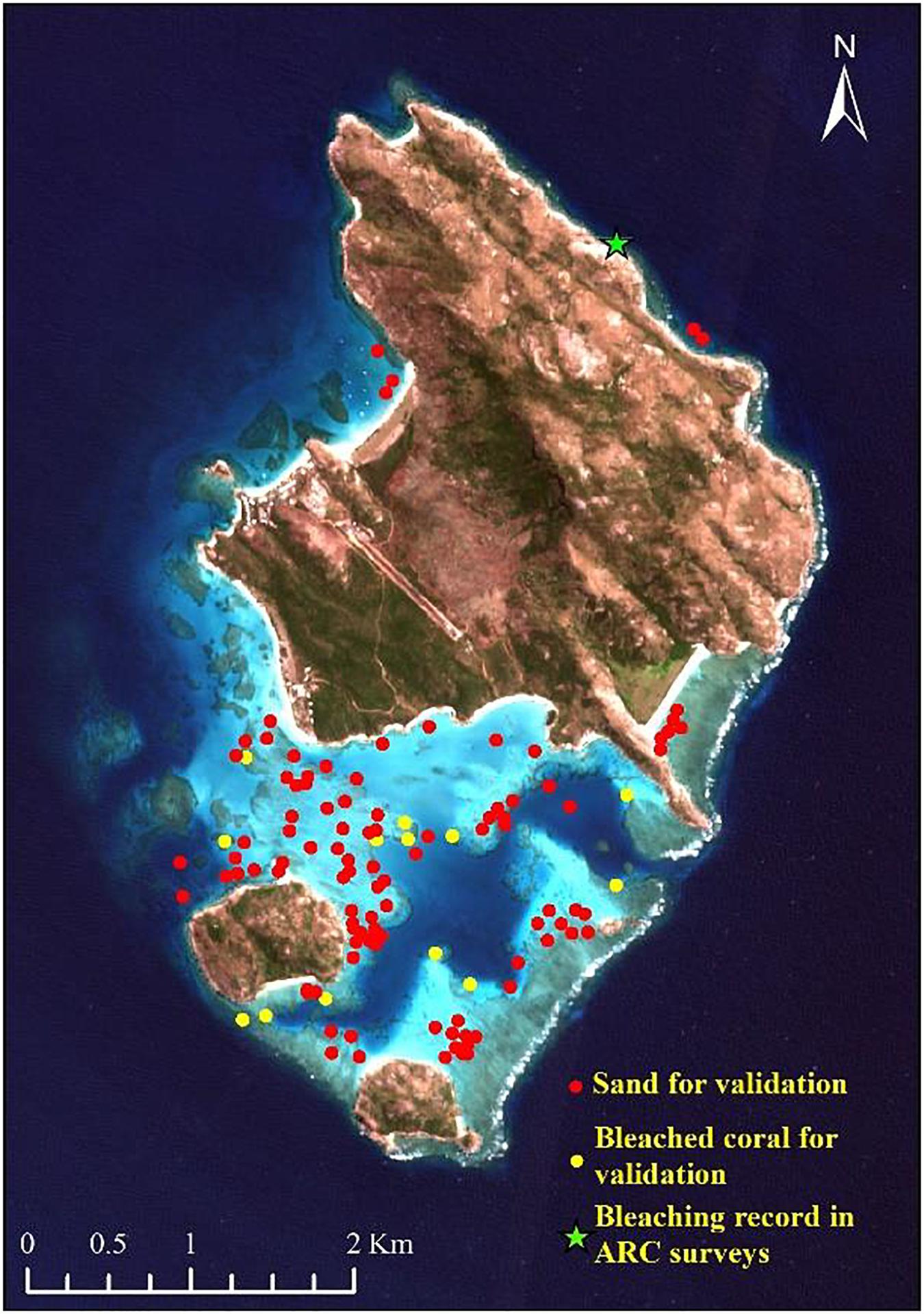
Figure 2. Ground truth points used for validation and accuracy assessment.

In the second method for change analysis, the time series images of depth invariant indices (DII) (Lyzenga, 1978; Green et al., 2000) were produced on different dates. The pixels that were successively classified as dark, bright, and dark substrates in the sequentially timed images can also provide information on coral bleaching. Please note that the dark substrates in this procedure are different from that in the PIFs. The dark substrates in the DII images refer to the bottom types that have a lower reflectance than sand or bleached corals, including seagrass, algae, and healthy corals. Workflow of the paper is illustrated in Figure 3 and the specific steps are described below.

FIGURE 3

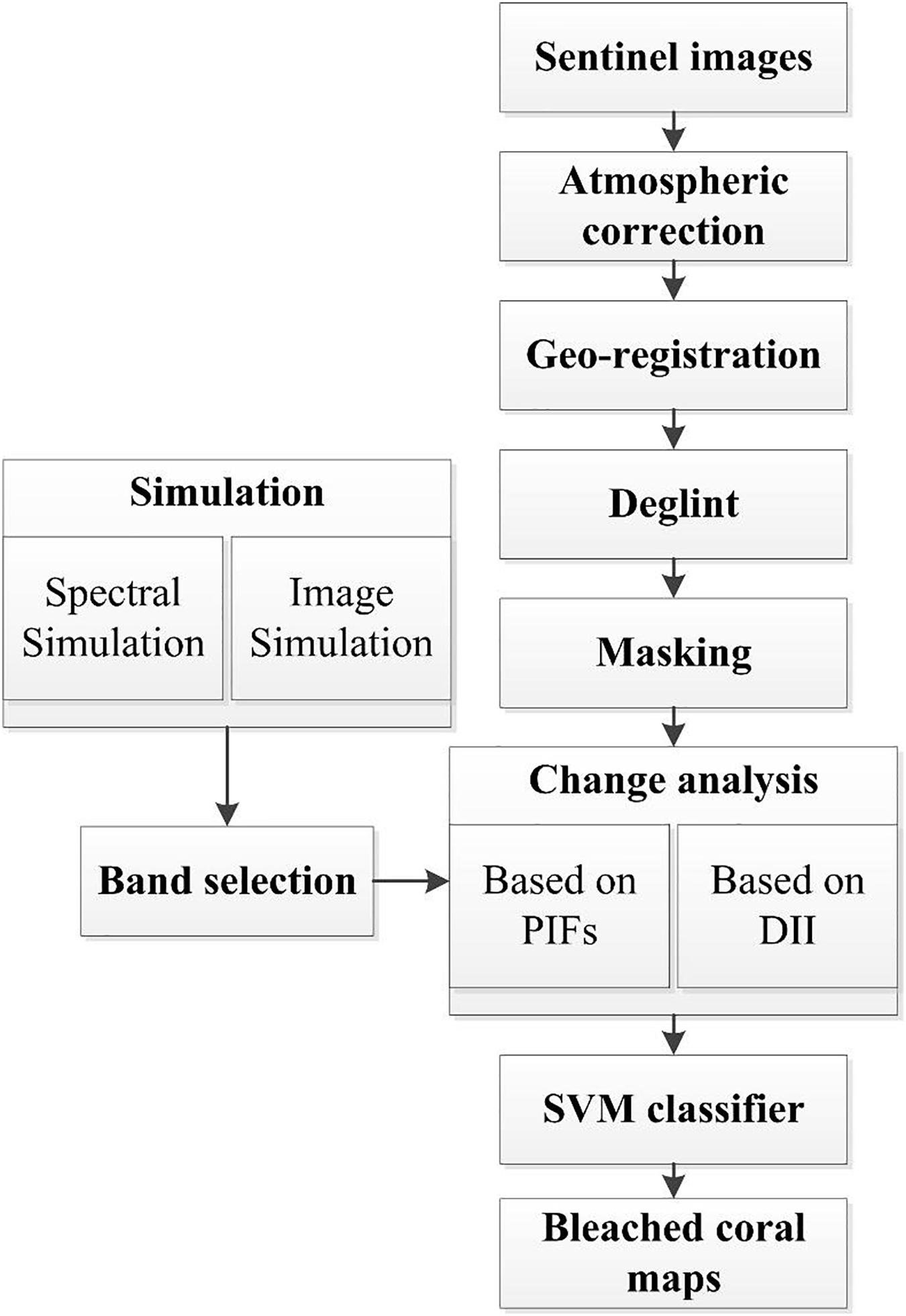
Figure 3. The overall workflow of the paper.

Spectral Simulation

It is widely believed that optical remote sensors have limited abilities for detecting underwater habitats because of water attenuation, which considerably affects the remote-sensed data of aquatic environments. The severity of attenuation differs with the electromagnetic wavelength. As the depth increases, the separability of habitat spectra declines. Although many marine habitat mapping studies have utilized water correction algorithms to compensate for the variable water depth, these algorithms are generally applicable to clear waters such as those in coral reef environments, at optically detectable depths. To evaluate the depth limit of Sentinel-2 bands for separating different substrates (sand, healthy coral, bleached coral, seagrass, and algae), the spectral values at different water depths were first simulated using the SA model (Lee et al., 1998, 1999). The environmental values used in the SA model are listed in Table 2. Many spectral measurements have demonstrated that the optical properties of major bottom types of coral reef in tropical oceanic environments are globally consistent (Kutser et al., 2020). Therefore, the in situ reflectance of different substrates was obtained from the spectral library measured by Roelfsema and Phinn (2012); Roelfsema et al. (2016), Roelfsema and Phinn (2017); Hochberg et al. (2003), and Xu J.P. et al. (2019). Several spectral curves for each substrate type were generalized to the typical one as input data to fulfill the simulation.

TABLE 2

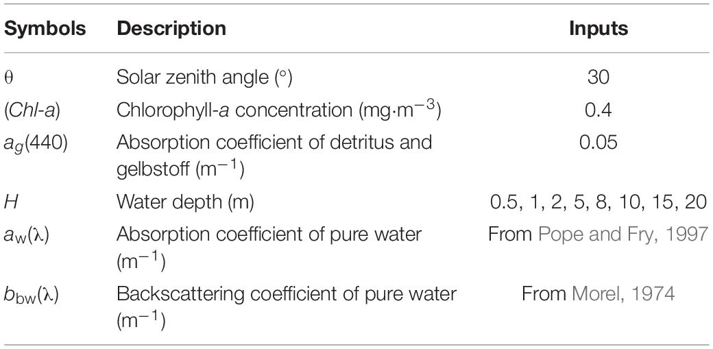
Table 2. Environmental inputs used in the SA model.

Image Simulation

Although hyperspectral reflectance can show distinguishable optical properties for different substrates, the features tend to be concealed when the reflectance signals turn into a multispectral image. For application to Sentinel-2A imagery, the in situ spectral reflectance for each target was convolved by the sensor’s RSR function of each band of Sentinel-2A:

$$Sig(\mathrm{\lambda }){}^{\prime }\frac{{\int }_{{\mathrm{\lambda }}_1}^{{\mathrm{\lambda }}_2}f(\mathrm{\lambda })R(\mathrm{\lambda })\mathit{d}\mathrm{\lambda }}{{\int }_{{\mathrm{\lambda }}_1}^{{\mathrm{\lambda }}_2}f(\mathrm{\lambda })\mathit{d}\mathrm{\lambda }}(1)$$

where Sig(λ)′ is the simulated image signal. R(λ) is the in situ spectral reflectance (%) or remote sensing reflectance (sr^–1). f(λ) is the average RSR function of Sentinel-2A that can be downloaded from European Space Agency (ESA) portal¹. Because of the strong water absorption in the red and near-infrared (NIR) bands, the Sentinel-2A image data was only simulated for bands 1, 2, 3, and 4, corresponding to 442.7, 492.4, 559.8, and 664.6 nm, respectively.

Atmospheric Correction

Atmospheric correction was performed for each image using the dark spectrum fitting (DSF) approach that allows for a smooth retrieval of atmospheric path reflectance over coastal and inland water applications (Vanhellemont and Ruddick, 2018; Vanhellemont, 2019). The DSF algorithm was bundled in the ACOLITE (Vanhellemont and Ruddick, 2014, 2015, 2016) software that can process bulk data from Landsat and Sentinel-2 in an automated and consistent manner. Then, the remote sensing reflectance (R_rs, sr^–1) was retrieved to be the output file as the Level-2A product. As the 13 bands in Sentinel-2 products have different spatial resolutions, the output resolution of Sentinel-2 products should be further resampled to a resolution of 10 m.

Geo-Registration, Deglint, and Masking

Although Sentinel-2 images have an overall satisfactory geometric positioning accuracy, there still exist some spatial mismatches among multi-temporal images. Several ground control points (GCPs) were selected from Google Earth to perform geometric corrections and geo-referencing in the images. In the lower latitude areas, the viewing geometry of the Sentinel-2 satellite makes it vulnerable to sun glint contamination. As the DSF selects the band with the lowest estimate of atmospheric path reflectance, the pixels and bands with severe sun glint are avoided when estimating atmospheric path reflectance. These pixels result in the presence of glint signals in the final surface reflectance (Vanhellemont, 2019). Brightness in a NIR band was utilized to deglint the visible wavelength bands based on the linear relationships between NIR and visible bands (Hedley et al., 2005). To facilitate further analysis, pixels containing boats, whitecaps (sea foam), clouds and their shadows, and land were masked (Gapper et al., 2019).

Radiometric Normalization Using Pseudo Invariant Features

The differences between images on two dates might be caused by the acquisition geometry of a scene, water column and/or atmospheric effects. For simplicity and practicability, two different images should be intercalibrated using the PIFs method proposed by Schott et al. (1988). The signals of PIF pixels of slave image are plotted versus those of reference image in each band. Fitting a linear equation to this plot defines a gain and offset to normalize slave image. This method works under the assumption that PIF pixels are constant over space and time. In this article, we selected sands and deep waters as PIF pixels. Basically, the method has the advantage of being inexpensive, requiring a small amount of processing time and depending little on data availability. A series of literature have demonstrated that this method is workable to correct water column effects, illumination effects, and atmospheric effects, such as in the applications of Michalek et al. (1993); Elvidge et al. (2004), and Zoffoli et al. (2014).

Depth Invariant Indices

This was done following the methods of Lyzenga (1978) and Green et al. (2000). It was based on the understanding that the attenuation of reflectance is approximately the inverse exponential with the water depth as follows:

$$Depth-invariantinde{x}_{ij}=\text{ln}\left(R_i\right)-(\frac{K_i}{K_j})\text{ln}\left(R_j\right)(2)$$

where R_i and R_j are the reflectance of band i and j, respectively. K_i/K_j is the ratio attenuation coefficient. For a unique substrate (sand), K_i/K_j is the gradient of the regression line that is generated by In(R_i) and In(R_j) at various depths. Bands 2 and 3 of Sentinel-2 were selected to calculate the DII.

Results and Discussion

Spectral Separability Analysis Based on Simulated Data

Spectral Separability of Different Substrates

Several studies have described the spectral characteristics of coral reef bottom types and discussed their spectral separability based on in situ spectral data or by simulating images of other satellites, such as Landsat, SPOT, IKONOS, etc. (Hochberg and Atkinson, 2000, 2003; Hochberg et al., 2003; Kutser et al., 2020). Therefore, the optical properties of the different substrates will not be analyzed in detail here. Figure 4 compares the typical spectral reflectance of different substrates and their values corresponding to the Sentinel-2A band settings. In general, sand has an overwhelming high reflectance for all bands, followed by bleached coral. Although in situ spectral data show that the specific reflectance of dark substrates (algae, healthy coral, and seagrass) range from 550 to 650 nm, these features are concealed and converted to similar or overlapping point values in the corresponding image data. As a result, all the dark substrates exhibit consistent features or subtle differences in the visible bands; thus, discriminating different dark substrates will be challenging from the Sentinel-2A data. In the absence of water absorption effects, both in situ and simulated spectral curves of bleached coral are fairly flat without any notable peaks or local minimum. The use of reflectance values is feasible for distinguishing bleached corals, with spectral curve generally above that of dark substrates but below that of sand. Note that Figure 4 shows the spectral reflectance of the pure endmembers. In the real word, the mixed reflectance of sand and dark substrates in one pixel might be similar to that of bleached coral, because most coral patches are a few meters in size, and the resolution of 10 m is clearly not sufficient for the signal collection of pure coral endmember. Compared with the other three bands, band 2 is preferable for capturing the change information because of the lower spatial resolution in band 1, lower variability in band 3 and stronger water absorption in band 4.

FIGURE 4

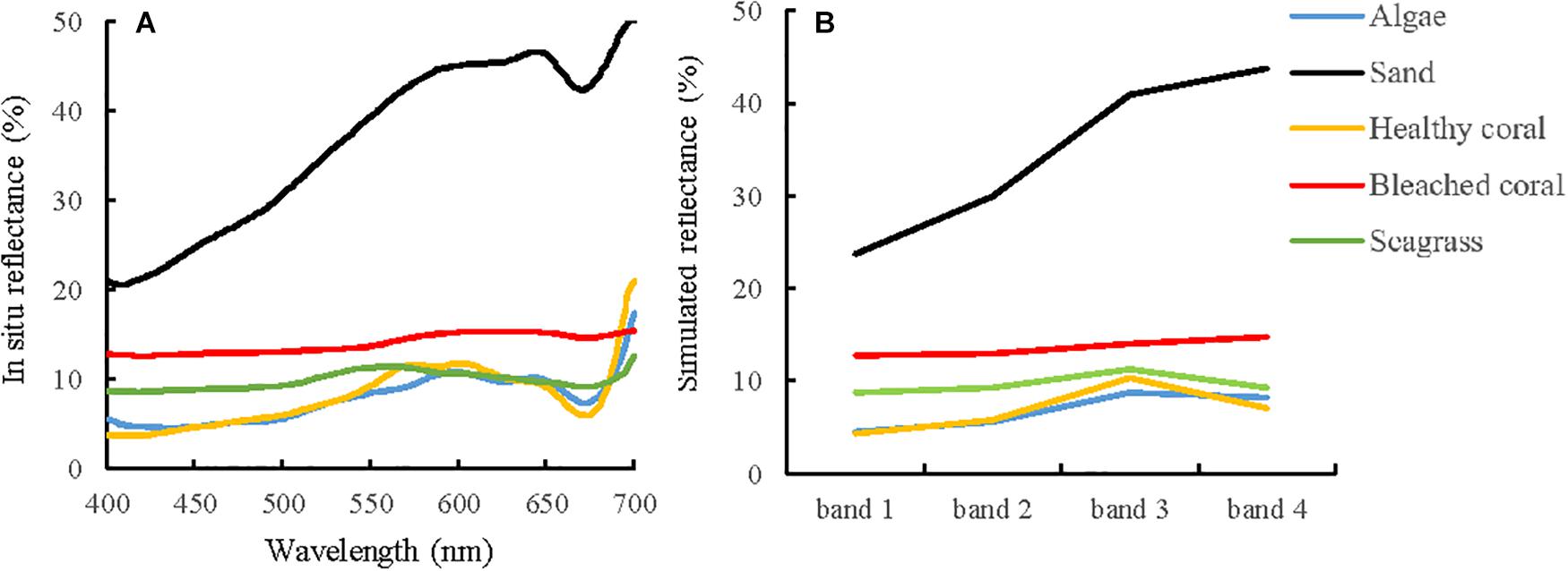
Figure 4. In situ measured reflectance and simulated image bands for different substrates. (A) Typical reflectance of substrates. The original spectral data came from spectral library measured by Roelfsema and Phinn (2012, 2016, 2017),Hochberg et al. (2003), and Xu J.P. et al. (2019), and were generalized to the typical one curve for each type of substrate. (B) Simulated reflectance of substrates based on RSR function of Sentmel-2A image over the Lizard Island. The red points of coral, sand, and deep water are part of ground truth data and will be used for the spectral analysis and classification training.

Spectral Reflectance of Bleached Corals at Different Severity

The mixed reflectance was calculated by a linear reflectance combination of healthy and bleached corals at different percentage. In Figure 5A, the triple-peaked feature in 550–650 nm tends to be subtle and finally disappears in the reflectance curve of bleached coral. With the increasing severity of coral bleaching, the in situ reflectance values exhibit an upward trend for almost the whole band, except for wavelengths above 693 nm.

FIGURE 5

Figure 5. Simulated reflectance of bleached coral at different severity. (A) Simulated reflectance based on in situ measured data, (B) simulated reflectance based on RSR function of Sentinel-2A.

In Figure 5B, although the reflectance increases consistently for all four bands with an increase in the percentage of bleached coral, band 3 displays a comparatively lower variability than the other three bands. Band 2 is found to be the best choice for detecting the change information during a coral bleaching event.

Spectral Separability at Different Water Depths

The spectral remote sensing reflectance of different substrates were simulated as a function of water depth (Figure 6) and then convolved by the sensor RSR function to find the corresponding image band values for Sentinel-2A (Figure 7). All the spectral curves at different water depths decreased from the red band because of the effect of strong water absorption. Although the increased water depth definitely reduces the signals in all bands, the degree of attenuation is different among the bands, and the reflectance discrepancy between the bright and dark substrates decreases.

FIGURE 6

Figure 6. Simulated Rrs of substrates at different water depths based on SA model.

FIGURE 7

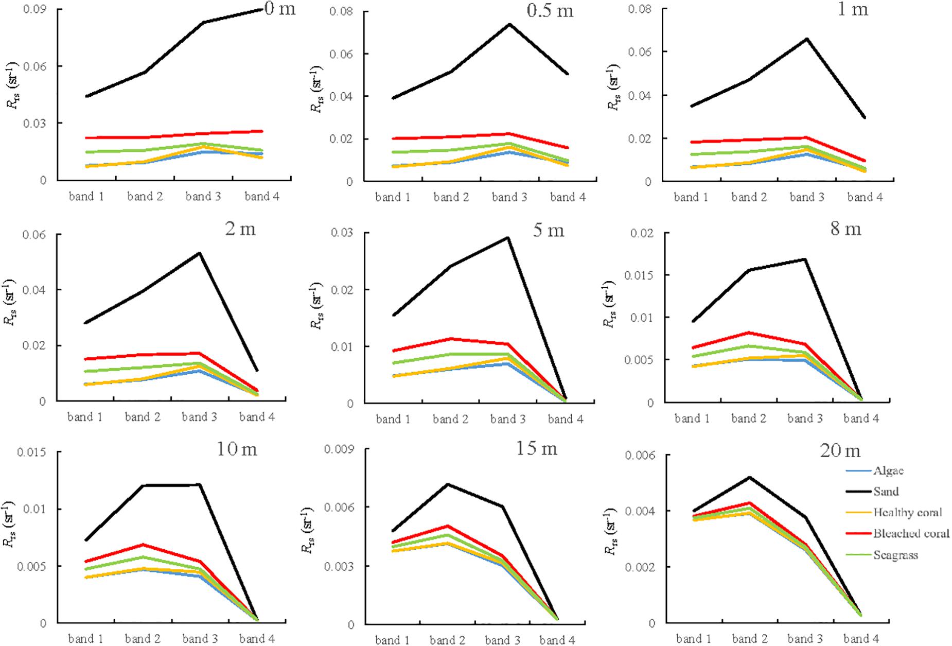
Figure 7. Simulated image values of substrates at different water depths based on spectral response function of Sentinel-2A.

In addition to the changes in the reflectance magnitude, there are some variations in the spectral shape. In Figure 6, all the spectral curves have a consistent shape at water depths of 0.5, 1, and 2 m; and they show a similar three-peaked feature from 500 to 600 nm when the depth is greater than 5 m. The first peak exceeds the other two when the water depth is 8 m and is maximum for all substrates when the depth is greater than 15 m. In Figure 7, a clear spectral concavity around band 2 can be observed for most substrates at depths of 0.5, 1, and 2 m; however, this becomes a convexity for depths greater than 5 m. Regardless of the water depth is, there exists a significant reflectance discrepancy between healthy and bleached corals, especially in band 2, which could be used to monitor bleached coral using change detection.

Although previous studies verified that Sentinel 2 images can detect bleaching in shallow waters (Hedley et al., 2012), the applicable water depth range was limited. The ratios of reflectance at different depths to the reflectance without water absorption effect are calculated. Table 3 summarizes the signal attenuation of bleached coral with increasing water depth considering these ratios. In general, band 2 has the lowest speed of light attenuation, followed by band 3 and band 1. It is clear that the signal at 10 m quickly dwindles to at most 30% of the original reflectance in band 2. The results also show that the NEΔR_E for bands 1, 2, 3, and 4 of Sentinel-2A were 0.00020, 0.00085, 0.00078, and 0.00069 sr^–1, respectively. It was assumed that coral bleaching could be detected if the signal difference was greater than at least twice the sensor noise (Yamano and Tamura, 2004). By calculating the reflectance differences of bleached and healthy corals in band 2 at different water depths, the results showed that the R_rs difference reduced to approximately 0.00211 sr^–1 at 10 m, and they were 0.00088 and 0.00037 sr^–1 for 15 and 20 m, respectively. This implies that the remote sensing of coral bleaching using Sentinel-2 is the best achieved at depths less than approximately 10 m.

TABLE 3

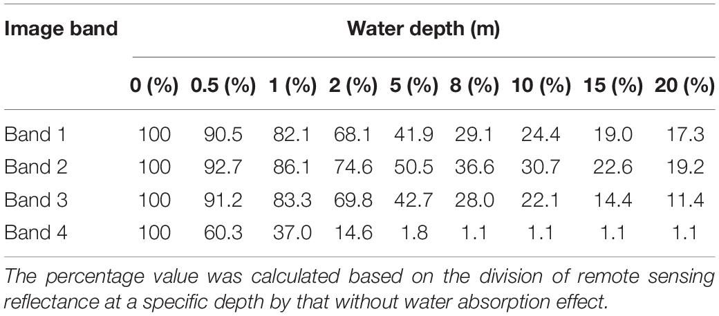
Table 3. Signal attenuation of bleached coral with increasing water depth.

Bleaching Detection

Spectral Variation of Reef Substrates Based on Change Analysis

To diagnose the spectral variation of different substrates over multi-temporal images, normalized remote sensing reflectance curves based on PIFs method were calculated and compared, because DII are not any forms of reflectance or radiance, but a relation between the signals in two spectral bands without a depth effect. Figure 8 shows the normalized R_rs of representative substrates (shallow sand, bleached coral, and deep water in Figure 1B taken on November 24, 2015. Because of the strong water absorption beyond the red part of spectrum, only the first four bands and band 8 (832.8 nm) were selected. Deep waters have the lowest values for all the bands. The shapes and magnitudes of these spectral curves are generally consistent with those in Figure 7. However, the reflectance of some coral sample points shows higher value than that of sand at band 1. This is probably because of the different water depths among these sample points, and this phenomenon appears to be more evident when the mixed pixel problem is severe in heterogeneous environments because of the low spatial resolution of band 1. The recommended band 2 was selected to carry out the change analysis because of its properties, that is, its relatively weak signal attenuation from water absorption and 10 m spatial resolution. Excluding areas with cloud cover, two deep waters and two shallow sand areas from visual interpretation, as well as four bleached corals from the ground truth data were selected randomly as representatives (Figure 1B). Figure 9 compares the R_rs and normalized R_rs for band 2. The spectral values are more regular after normalization. In general, the curves of shallow sand and deep water are comparatively stable without notable changing trend over the time series, whereas all four curves that have experienced coral bleaching are characterized with an initial increase and a subsequent decrease, which corresponds to the signal change of bleached coral. The curve magnitudes pre- and post-bleaching are intermediate between that of shallow sand and deep waters; however, the maximum values are observed for the images taken in March 2016. This is consistent with the results of several reports that the study area experienced a serious bleaching event in the summer of 2016 (Great Barrier Reef Marine Park Authority, 2017; Hughes et al., 2017). The maximum values of bleached corals on March 23, 2016 are approximately similar to that of shallow sand, implying that it is impossible to discriminate bleached coral from shallow sand based on only one image.

FIGURE 8

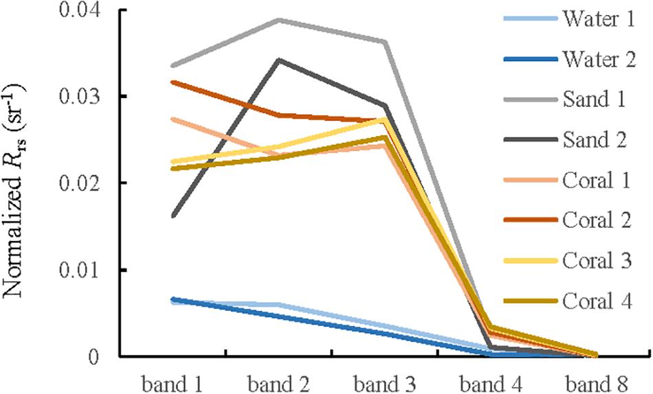
Figure 8. Normalized Rrs of representative substrates taken on November 24, 2015.

FIGURE 9

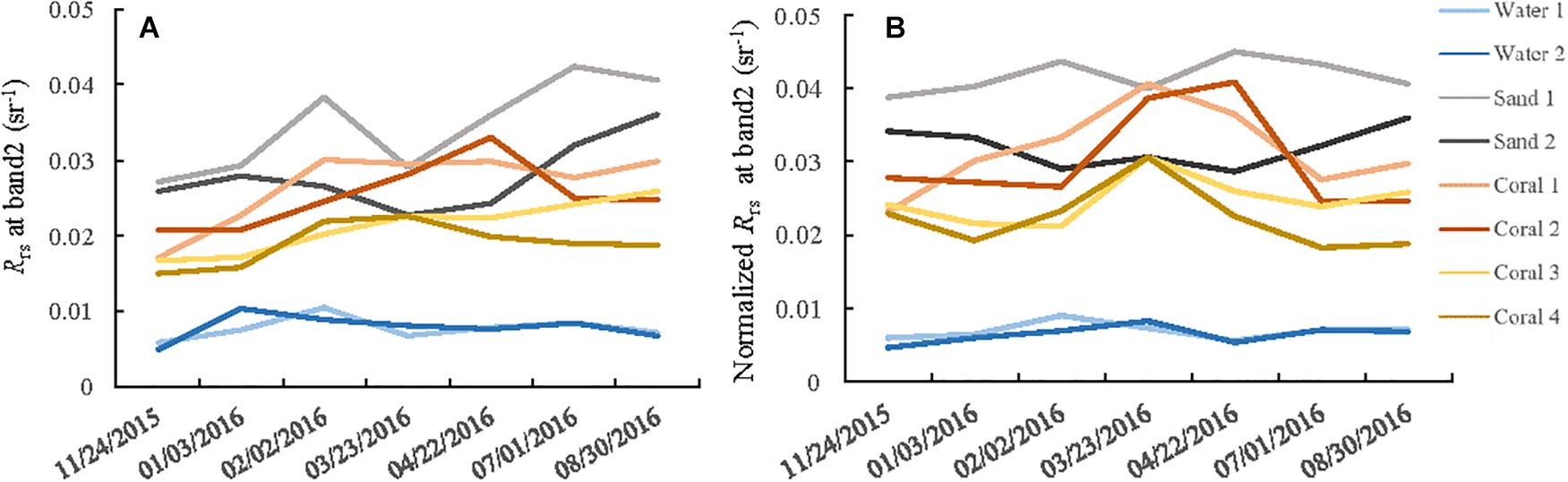
Figure 9. Reflectance curves of representative substrates over multi-temporal images. (A) R_rs obtained after atmospheric correction and deglint. (B) Normalized R_rs using PIFs method.

Bleached Corals Mapping

Three normalized images taken on November 24, 2015, March 23, 2016, and August 30, 2016, corresponding to the spectral turning points of bleached corals, were selected for the change analysis. Four points of bleached corals in Figure 1B were selected randomly from ground truth data and then used to train the SVM model.

Figure 10 maps the bleached corals identified from the multi-temporal normalized images and DII images. From the reef top, 57,694 pixels (5.77 km²) were involved in the classification of processed images. Subsequently, 4592 pixels (0.46 km²) and 10,594 pixels (1.06 km²) were identified as having experienced coral bleaching based on the PIFs and DII methods, respectively. In contrast, the bleached area recognized by the DII method was almost twice that of the PIFs method. Most bleached corals were distributed in the southern reef top because there was a large area of shallow reef, and the northeast and northwest banks were seriously affected by white cap or clouds. Actually, some of the bleaching was conspicuous enough to show up in the time series images by view interpretation. The zoomed-in areas in three colored rectangles in Figure 11 show significant brightness changes. The corals in the rectangles of March are much brighter than that of the other two images. The benthic data obtained by Roelfsema et al. (2014) in 2011 and 2012 indicated an approximate area of 4.45 km² of hard coral related classes (coral reef matrix, reef matrix coral, rubble coral, and sand rubble coral/algae). Surveys by the Australian Institute of Marine Science (AIMS) Long-Term Monitoring Program (LTMP) and the Marine Monitoring Program (MMP) indicated that the average percentage cover of hard coral decreased from 25% in 2013 to 8% in 2015². Therefore, if the coral decline proportion was used to deduce the hard coral coverage data in 2015, the rough percentage of bleached corals noted here would be 32 and 74% according to the PIFs and DII methods, respectively. The first percentage is generally consistent with the aerial scores of bleaching severity in the Aerial Survey Data collected by ARC; however, the second percentage is slightly bigger than that in the survey.

FIGURE 10

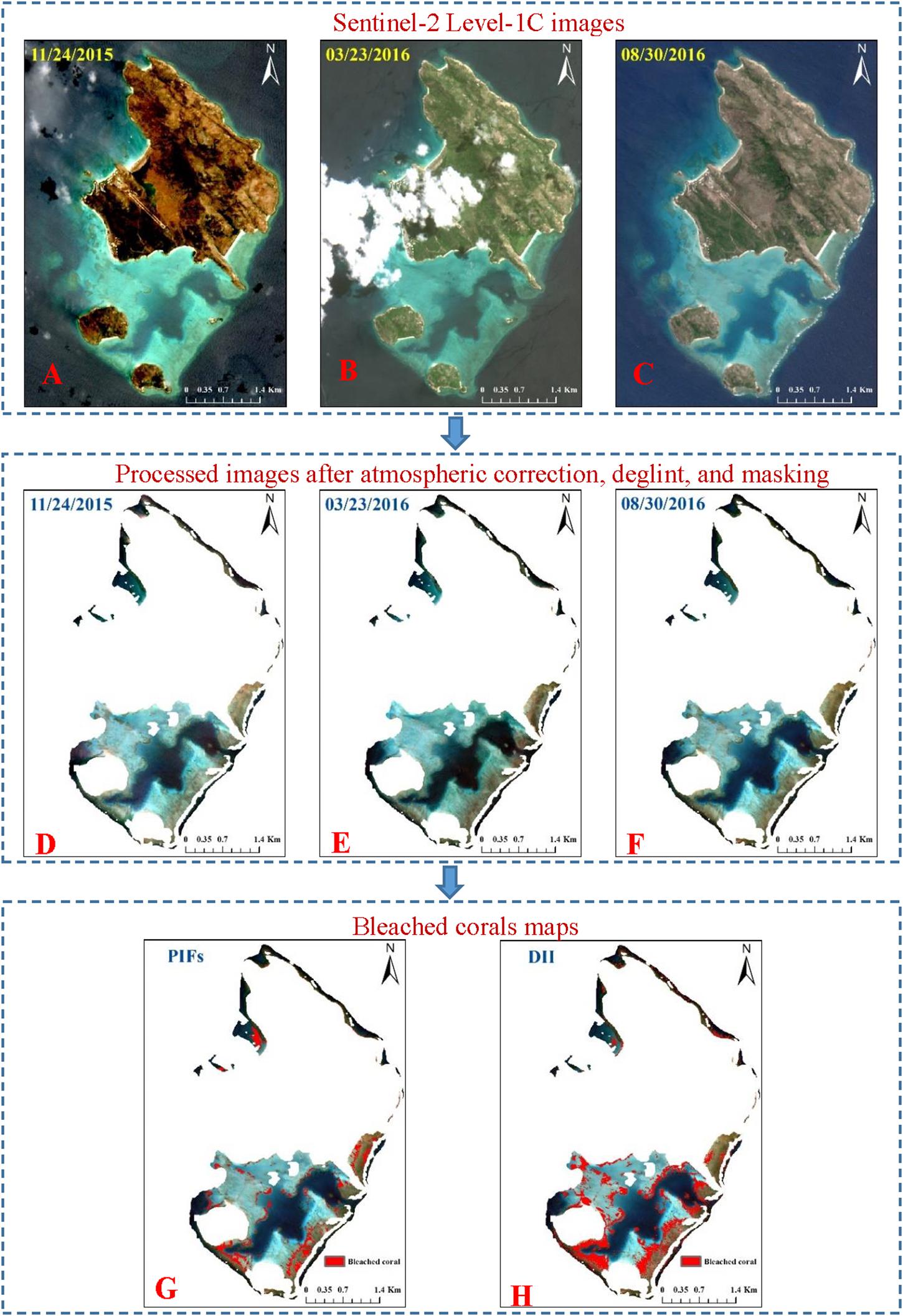
Figure 10. Bleached corals maps of reef top of the Lizard Island based on change analysis. Panels (A–C) are original Sentinel-2 Level-lC images. Panels (D–F) are processed images after atmospheric correction, deglint, and masking. Masked areas are locations contaminated by boats, cloud, cloud shadow, land, white cap in any scene for the three images. Panels (G,H) are bleached corals maps based on PIFs and DII methods, respectively.

FIGURE 11

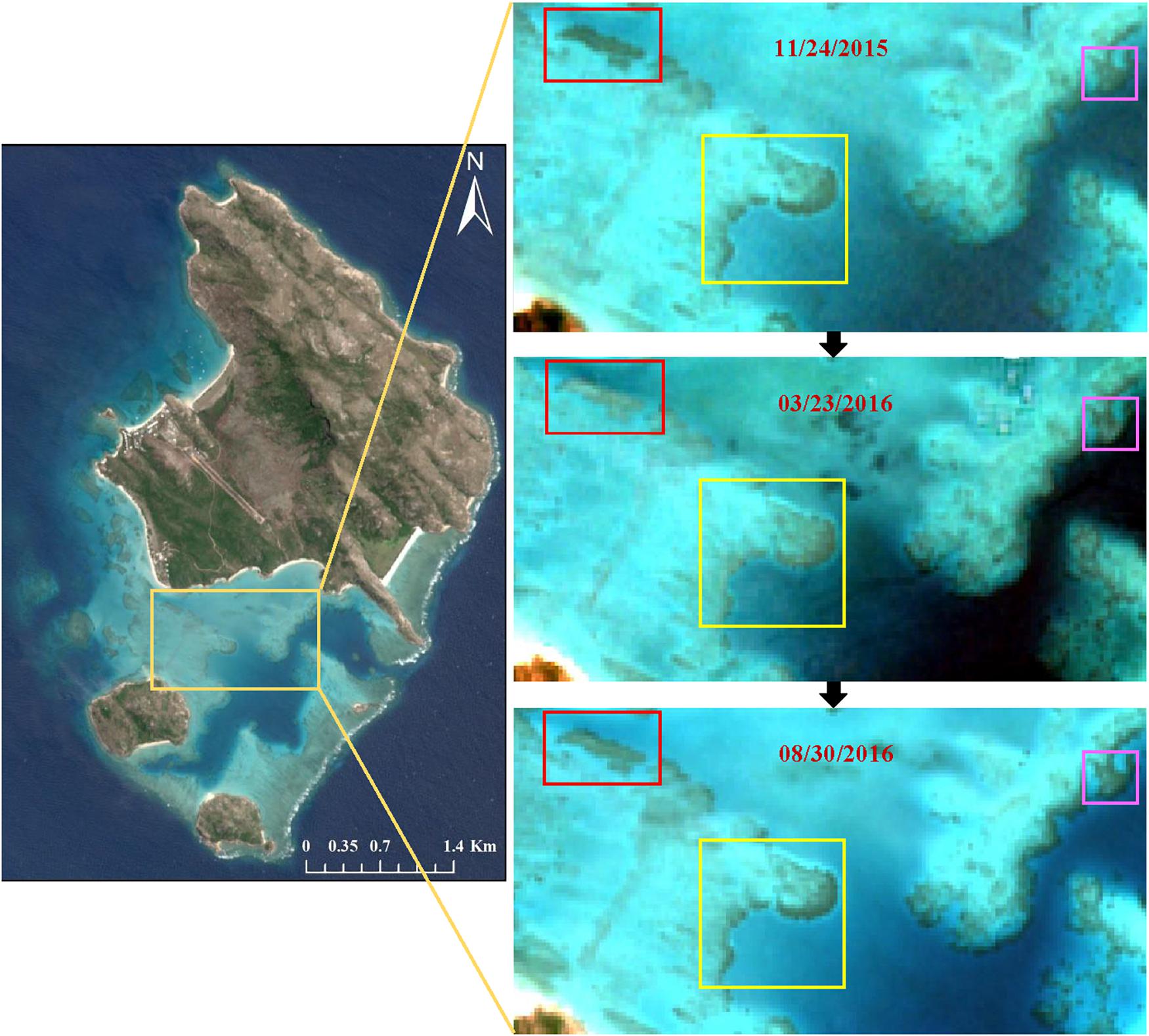
Figure 11. Three areas of clear coral bleaching as visible in March 2016, compared with images taken in November 2015 and August 2016. All the images are the RGB composites of bands 4, 3, and 2 after data pre-processing, including atmospheric correction and PIFs normalization.

Accuracy Assessment

The bleached corals maps created by the PIFs and DII approaches had an overall accuracy of 88.9 and 57.1%, respectively. Table 4 summarizes their user’s and producer’s accuracies. The unrecognized bleached corals were mainly located at the fore reef with a relatively great water depth. The lower user’s accuracy achieved by the DII was mainly attributed to the misclassification of many sand/rubble areas as bleached corals.

TABLE 4

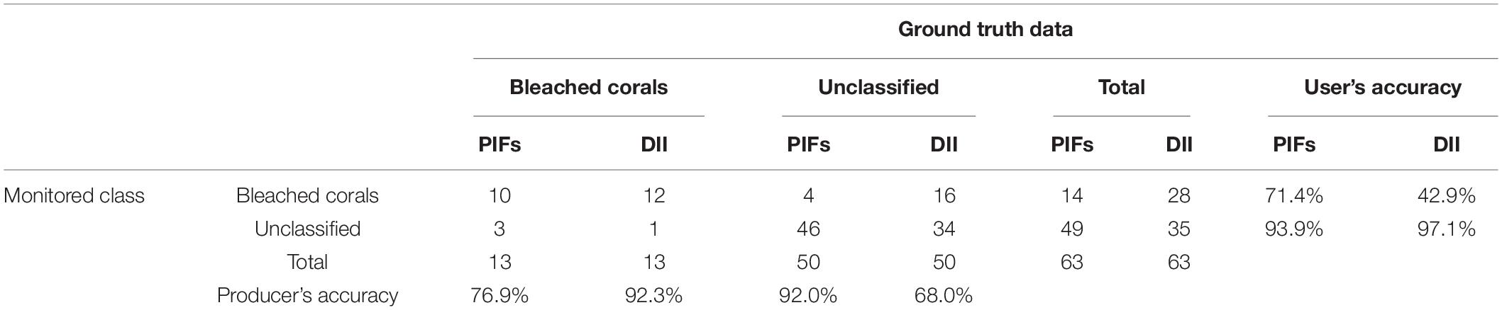
Table 4. Confusion matrix calculated for the Lizard Island bleached corals map based on PIFs and DII methods.

However, when the change analysis was carried out again based on the DII multi-temporal images with an additional PIFs normalization before calculating the DII, the bleached corals map showed no significant improvement. Figure 12 compares the DII images with original band 2 images, showing that the transformation makes the DII images considerably coarser and introduces some extra noise that would exert a negative influence on the change analysis, especially when the images are somewhat obscure without sufficiently high clarity.

FIGURE 12

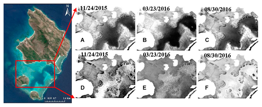
Figure 12. Comparison of DII images with processed band 2 images after atmospheric correction, deglint, and masking. Panels (A–C) are the processed band 2 images on different dates, whereas panels (D–F) are the corresponding DII images.

To compare the results from two images of different dates, the change analysis was performed using the images taken on November 24, 2015 and March 23, 2016. The map in Figure 13 shows a larger coverage of bleached corals compared with Figure 10G. Although the images taken on two dates could identify most bleached corals, the map accuracy was not satisfactory (overall accuracy of 50.7%) because considerable sand/rubble was misclassified as bleached corals. In most cases, the image resolution of 10 m still cannot capture the spatial variability in highly heterogeneous reef environment, and pixels discerned as corals are mostly mixed pixels containing corals at different percentages. This will weaken the change signals coming from bleached corals and result in a great uncertainty in the final classification. However, this uncertainty can be partly reduced by introducing an image taken on a different date because bleached corals would recover from bleaching or be overgrown by some algae with another featured signal change. Performing feature matching again with sample points in the third image eliminates some misclassifications and improves the accuracy.

FIGURE 13

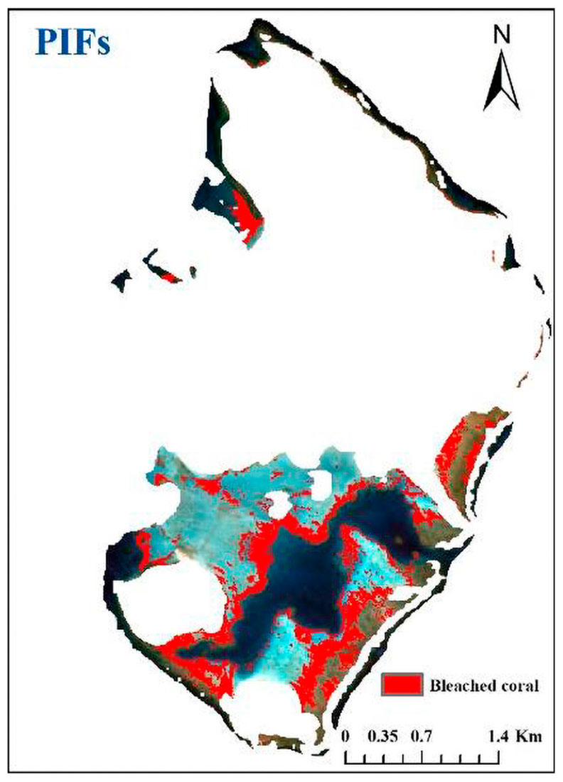
Figure 13. Bleached corals map created by PIFs method with two images taken on November 24, 2015 and March 23, 2016.

Conclusion

Sentinel-2 can provide essential information for coral reef monitoring applications. It has a good spatial resolution and revisit time, which should enable the change analysis for the remote sensing of coral bleaching because a single image is not sufficient for identifying bleached corals. The spectral and image simulations confirmed that band 2 is the most suitable band for obtaining change information during a coral bleaching event. The detection capability of Sentinel-2 is limited by water depth. It exhibits the best performance at depths less than 10 m. The change analysis of the multi-temporal Sentinel-2 images was used to monitor bleached corals at the Lizard Island, Australia. The results showed that the normalization method based on PIFs is superior to that using DII. The utilization of a third image in the change analysis corresponding to the period when corals recovered from bleaching or were overgrown by algae improved the classification accuracy. The proposed methodology is generally feasible approach for remote sensing of coral bleaching. It also provides insight into benthic changes for further studies related to climate changes or ecological planning. However, observations in this article were limited in space and may not sufficient to identify coral bleaching in the regional or global scales. In order to optimize the method, analysis of long time series data in different regions is essential to capture the temporal features of coral changes in bleaching events. In addition, new methods of artificial Intelligence, such as deep learning, are recommended in the future applications of benthos classification. Change analysis incorporating other marine environmental information, such as sea surface temperature, UV irradiance, wave exposure, ocean color, carbonate chemistry, etc., will also be helpful to detect and forecast bleaching.

Data Availability Statement

The datasets presented in this study can be found in online repositories. The names of the repository/repositories and accession number(s) can be found in the article/supplementary material.

Author Contributions

JX designed the manuscript structure and drafted the manuscript. JZ and ZL contributed to the concepts and methods of remote sensing of coral bleaching. FW and YC processed and analyzed the data. All authors contributed to the data processing, analyses, and final writing.

Funding

This work was supported by the National Natural Science Foundation of China (No. 41871281), State Scholarship Fund (No. 201909210002), and the National Key Research and Development Program of China (Nos. 2019YFC1407904 and 2018YFC1407605).

Conflict of Interest

The authors declare that the research was conducted in the absence of any commercial or financial relationships that could be construed as a potential conflict of interest.

Acknowledgments

We thank Terry Hughes for providing the Aerial Survey Data of Great Barrier Reefs in 2016. We also thank Quinten Vanhellemont for his help in the processing of Sentinel images.

Footnotes

1. ^ https://sentinels.copernicus.eu/web/sentinel/user-guides/sentinel-2-msi/document-library/-/asset_publisher/Wk0TKajiISaR/content/sentinel-2a-spectral-responses
2. ^ http://apps.aims.gov.au/reef-monitoring/reef/14116S

References

Andréfouët, S., Berkelmans, R., Odriozola, L., Done, T., Oliver, J., and Müller-Karger, F. (2002). Choosing the appropriate spatial resolution for monitoring coral bleaching events using remote sensing. Coral Reefs 21, 147–154. doi: 10.1007/s00338-002-0233-x

CrossRef Full Text | Google Scholar

Barkley, H. C., Cohen, A. C., Mollica, N. R., Brainard, R. E., Rivera, H. E., DeCarlo, T. M., et al. (2018). Repeat bleaching of a central Pacific coral reef over the past six decades (1960-2016). Commun. Biol. 177, 1–10.

Google Scholar

Brando, V. E., Anstee, J. M., Wettle, M., Dekker, A. G., Phinn, S. R., and Roelfsema, C. R. (2009). A physics based retrieval and quality assessment of bathymetry from suboptimal hyperspectral data. Rem. Sens. Environ. 113, 755–770. doi: 10.1016/j.rse.2008.12.003

CrossRef Full Text | Google Scholar

Clark, C. D., Mumby, P. J., Chisholm, J. R. M., Jaubert, J., and Andréfouët, S. (2010). Spectral discrimination of coral mortality states following a severe bleaching event. Int. J. Rem. Sens. 21, 2321–2327. doi: 10.1080/01431160050029602

CrossRef Full Text | Google Scholar

Daly, M. (2005). Wave Energy and Shoreline Response on a Fringing Reef Complex, Lizard Island, Qld, Australia. 105., Ph. D. Thesis, University of New South Wales, Sydney, NSW.

Google Scholar

Douglas, A. E. (2003). Coral bleaching-how and why? Mar. Pollut. Bull. 46, 385–392. doi: 10.1016/s0025-326x(03)00037-7

CrossRef Full Text | Google Scholar

Elvidge, C. D., Dietz, J. B., Berkelmans, R., Andréfouët, S., Skirving, W., Strong, A. E., et al. (2004). Satellite observation of Keppel Islands (Great Barrier Reef) 2002 coral bleaching using IKONOS data. Coral Reefs 23, 123–132. doi: 10.1007/s00338-003-0364-8

CrossRef Full Text | Google Scholar

Gapper, J. J., El-Askary, H., Linstead, E., and Piechota, T. (2019). Coral reef changes detection in remote Pacific islands using support vector machine classifiers. Rem. Sens. 11:1525. doi: 10.3390/rs11131525

CrossRef Full Text | Google Scholar

Great Barrier Reef Marine Park Authority (2017). Final Report: 2016 Coral Bleaching Event on the Great Barrier Reef. Townsville, QLD: GBRMPA.

Google Scholar

Green, E., Mumby, P., Edwards, A., and Clark, C. (2000). Remote Sensing: Handbook for Tropical Coastal Management. Paris: UNESCO.

Google Scholar

Hamylton, S. M., Leon, J. X., Saunders, M. I., and Woodroffe, C. D. (2014). Simulating reef response to sea-level rise at Lizard Island: a geospatial approach. Geomorphology 222, 151–161. doi: 10.1016/j.geomorph.2014.03.006

CrossRef Full Text | Google Scholar

Hedley, J. C., Roelfsema, I., Chollett, A., Harborne, S., Heron, S., Weeks, W., et al. (2016). Remote sensing of coral reefs for monitoring and management: a review. Rem. Sens. 8:118. doi: 10.3390/rs8020118

CrossRef Full Text | Google Scholar

Hedley, J. D., Harborne, A. R., and Mumby, P. J. (2005). Technical note: simple and robust removal of sun glint for mapping shallow−water benthos. Int. J. Rem. Sens. 26, 2107–2112. doi: 10.1080/01431160500034086

CrossRef Full Text | Google Scholar

Hedley, J. D., Roelfsema, C., Brando, V., Giardino, C., Kutser, T., Phinn, S., et al. (2018). Coral reef applications of Sentinel-2: coverage, characteristics, bathymetry and benthic mapping with comparison to Landsat 8. Rem. Sens. Environ. 216, 598–614. doi: 10.1016/j.rse.2018.07.014

CrossRef Full Text | Google Scholar

Hedley, J. D., Roelfsema, C., Koetz, B., and Phinn, S. (2012). Capability of Sentinel 2 mission for tropical coral reef mapping and coral bleaching detection. Rem. Sens. Environ. 120, 145–155. doi: 10.1016/j.rse.2011.06.028

CrossRef Full Text | Google Scholar

Hochberg, E. J., and Atkinson, M. J. (2000). Spectral discrimination of coral reef benthic communities. Coral Reefs 19, 164–171. doi: 10.1007/s003380000087

CrossRef Full Text | Google Scholar

Hochberg, E. J., and Atkinson, M. J. (2003). Capabilities of remote sensors to classify coral, algae and sand as pure and mixed spectra. Rem. Sens. Environ. 85, 174–189. doi: 10.1016/s0034-4257(02)00202-x

CrossRef Full Text | Google Scholar

Hochberg, E. J., Atkinson, M. J., and Andréfouët, S. (2003). Spectral reflectance of coral reef bottom-types worldwide and implications for coral reef remote sensing. Rem. Sens. Environ. 85, 159–173. doi: 10.1016/s0034-4257(02)00201-8

CrossRef Full Text | Google Scholar

Hughes, T. P., Anderson, K. D., Connolly, S. R., Heron, S. F., Kerry, J. T., Lough, J. M., et al. (2018a). Spatial and temporal patterns of mass bleaching of corals in the Anthropocene. Science 359, 80–83. doi: 10.1126/science.aan8048

PubMed Abstract | CrossRef Full Text | Google Scholar

Hughes, T. P., Kerry, J. T., Álvarez-Noriega, M., Álvarez-Romero, J. G., Anderson, K. D., Baird, A. H., et al. (2017). Global warming and recurrent mass bleaching of corals. Nature 543, 373–377.

Google Scholar

Hughes, T. P., Kerry, J. T., and Simpson, T. (2018b). Large-scale bleaching of corals on the Great Barrier Reef. Ecology 99:501. doi: 10.1002/ecy.2092

PubMed Abstract | CrossRef Full Text | Google Scholar

Kutser, T., Hedley, J., Giardino, C., Roelfsema, C., and Brando, V. E. (2020). Remote sensing of shallow waters – A 50 year retrospective and future directions. Rem. Sens. Environ. 240, 1–18. doi: 10.1016/j.rse.2014.09.021

CrossRef Full Text | Google Scholar

Lee, Z. P., Carder, K. L., Mobley, C. D., Steward, R. G., and Patch, J. S. (1998). Hyperspectral remote sensing for shallow waters. I. A semianalytical model. Appl. Opt. 37, 6329–6338. doi: 10.1364/ao.37.006329

PubMed Abstract | CrossRef Full Text | Google Scholar

Lee, Z. P., Carder, K. L., Mobley, C. D., Steward, R. G., and Patch, J. S. (1999). Hyperspectral remote sensing for shallow waters. II. Deriving bottom depths and water properties by optimization. Appl. Opt. 38, 3831–3843. doi: 10.1364/ao.38.003831

PubMed Abstract | CrossRef Full Text | Google Scholar

Leon, J. X., and Woodroffe, C. D. (2011). Improving the synoptic mapping of coral reef geomorphology using object-based image analysis. Int. J. Geogr. Inform. Sci. 25, 949–969. doi: 10.1080/13658816.2010.513980

CrossRef Full Text | Google Scholar

Lyzenga, D. R. (1978). Passive remote sensing techniques for mapping water depth and bottom features. Appl. Opt. 17, 379–383. doi: 10.1364/ao.17.000379

PubMed Abstract | CrossRef Full Text | Google Scholar

Lyzenga, D. R. (1981). Remote sensing of bottom reflectance and water attenuation parameters in shallow water using aircraft and Landsat data. Int. J. Remote Sens. 2, 71–82. doi: 10.1080/01431168108948342

CrossRef Full Text | Google Scholar

Michalek, J. L., Wagner, T. W., Luzkovich, J. J., and Stoffle, R. W. (1993). Multispectral change vector analysis for monitoring coastal marine environments. Photogramm. Eng. Remote Sens. 59, 381–384.

Google Scholar

Morel, A. (1974). “Optical properties of pure water and pure sea waters,” in Optical Aspects of Oceanography, eds N. G. Jerlov and E. S. Nielsen (New York, NY: Academic Press), 1–24.

Google Scholar

Mumby, P. J., Green, E. P., Edwards, A. J., and Clark, C. D. (1999). The cost-effectiveness of remote sensing for tropical coastal resources assessment and management. J. Environ. Manag. 55, 157–166. doi: 10.1006/jema.1998.0255

CrossRef Full Text | Google Scholar

Philipson, P., and Lindell, T. (2003). Can coral reefs be monitored from space? Ambio 32, 586–593. doi: 10.1579/0044-7447-32.8.586

PubMed Abstract | CrossRef Full Text | Google Scholar

Phinn, S. R., Roelfsema, C. M., and Mumby, P. J. (2012). Multi-scale, object based image analysis for mapping geomorphic and ecological zones on coral reefs. Int. J. Rem. Sens. 33, 3768–3797. doi: 10.1080/01431161.2011.633122

CrossRef Full Text | Google Scholar

Pope, R., and Fry, E. (1997). Absorption spectrum (380-700 nm) of pure waters: II. Integrating cavity measurements. Appl. Opt. 36, 8710–8723. doi: 10.1364/ao.36.008710

PubMed Abstract | CrossRef Full Text | Google Scholar

Roelfsema, C., Kovacs, E., Ortiz, J. C., Wolff, N. H., Callaghan, D., Wettle, M., et al. (2018). Coral reef habitat mapping: a combination of object-based image analysis and ecological modelling. Rem. Sens. Environ. 208, 27–41. doi: 10.1016/j.rse.2018.02.005

CrossRef Full Text | Google Scholar

Roelfsema, C. M., and Phinn, S. R. (2012). Spectral Reflectance Library of Selected Biotic and Abiotic Coral Reef Features in Heron Reef. Brisbane, QLD: University of Queensland, doi: 10.1594/PANGAEA.804589

CrossRef Full Text | Google Scholar

Roelfsema, C. M., and Phinn, S. R. (2017). Spectral Reflectance Library of Healthy and Bleached Corals in the Keppel Islands, Great Barrier Reef. Bremen: PANGAEA, doi: 10.1594/PANGAEA.872507

CrossRef Full Text | Google Scholar

Roelfsema, C. M., Phinn, S. R., and Joyce, K. (2016). Spectral Reflectance Library of Algal, Seagrass and Substrate Types in Moreton Bay, Australia. Bremen: PANGAEA, doi: 10.1594/PANGAEA.864310

CrossRef Full Text | Google Scholar

Roelfsema, C. M., Phinn, S. R., Jupiter, S., Comley, J., and Albert, S. (2013). Mapping coral reefs at reef to reef-system scales (10–600 km2) using OBIA driven ecological and geomorphic principles. Int. J. Rem. Sens. 34, 6367–6388. doi: 10.1080/01431161.2013.800660

CrossRef Full Text | Google Scholar

Roelfsema, C. M., Saunders, M. I., Canto, R. F. C., Leon, J. X., Phinn, S. R., and Hamylton, S. (2014). Habitat Map for Lizard Island reef, Australia Derived from a Photo-transect Survey Field Data Collected in December 2011 and September/October 2012. Bremen: PANGAEA, doi: 10.1594/PANGAEA.864209

CrossRef Full Text | Google Scholar

Schott, J. R., Salvaggio, C., and Volchok, W. J. (1988). Radiometric scene normalization using pseudoinvariant features. Rem. Sens. Environ. 26, 1–16. doi: 10.1016/0034-4257(88)90116-2

CrossRef Full Text | Google Scholar

Tebbett, S. B., Streit, R. P., and Bellwood, D. R. (2019). Expansion of a colonial ascidian following consecutive mass coral bleaching at Lizard Island, Australia. Mar. Environ. Res. 144, 125–129. doi: 10.1016/j.marenvres.2019.01.007

PubMed Abstract | CrossRef Full Text | Google Scholar

Vanhellemont, Q. (2019). Adaptation of the dark spectrum fitting atmospheric correction for aquatic applications of the Landsat and Sentinel-2 archives. Rem. Sens. Environ. 225, 175–192. doi: 10.1016/j.rse.2019.03.010

CrossRef Full Text | Google Scholar

Vanhellemont, Q., and Ruddick, K. (2014). Turbid wakes associated with offshore wind turbines observed with Landsat 8. Rem. Sens. Environ. 145, 105–115. doi: 10.1016/j.rse.2014.01.009

CrossRef Full Text | Google Scholar

Vanhellemont, Q., and Ruddick, K. (2015). Advantages of high quality SWIR bands for ocean colour processing: examples from Landsat-8. Rem. Sens. Environ. 161, 89–106. doi: 10.1016/j.rse.2015.02.007

CrossRef Full Text | Google Scholar

Vanhellemont, Q., and Ruddick, K. (2016). “ACOLITE for sentinel-2: aquatic applications of MSI imagery,” in ESA Special Publication SP-740. Presented at the 1 Living Planet Symposium Held in Prague, Czech Republic, (Prague: European Space Agency).

Google Scholar

Vanhellemont, Q., and Ruddick, K. (2018). Atmospheric correction of metre-scale optical satellite data for inland and coastal water applications. Rem. Sens. Environ. 216, 586–597. doi: 10.1016/j.rse.2018.07.015

CrossRef Full Text | Google Scholar

Wettle, M., Brando, V., and Dekker, A. (2004). A methodology for retrieval of environmental noise equivalent spectra applied to four Hyperion scenes of the same tropical coral reef. Rem. Sens. Environ. 93, 188–197. doi: 10.1016/j.rse.2004.07.014

CrossRef Full Text | Google Scholar

Wismer, S., Tebbett, S. B., Streit, R. P., and Bellwood, D. R. (2019). Spatial mismatch in fish and coral loss following 2016 mass coral bleaching. Sci. Total Environ. 650, 1487–1498. doi: 10.1016/j.scitotenv.2018.09.114

PubMed Abstract | CrossRef Full Text | Google Scholar

Xu, H., Liu, Z., Zhu, J., Lu, X., and Liu, Q. (2019). Classification of coral reef benthos around Ganquan Island using WorldView-2 satellite imagery. J. Coast. Res. 93, 466–474. doi: 10.2112/si93-061.1

CrossRef Full Text | Google Scholar

Xu, J. P., Li, F., Meng, Q. H., and Wang, F. (2019). The analysis of spectral separability of different coral reef benthos and the influence of pigments on coral spectra based on in situ data. Spectrosc. Spect. Anal. 39, 2462–2469.

Google Scholar

Xu, J. P., Zhao, J. H., Li, F., Wang, L., Song, D. R., Wen, S. Y., et al. (2016). Object-based image analysis for mapping geomorphic zones of coral reefs in the Xisha Islands, China. Acta Oceanol. Sin. 35, 19–27. doi: 10.1007/s13131-016-0921-y

CrossRef Full Text | Google Scholar

Yamano, H., and Tamura, M. (2004). Detection limits of coral reef bleaching by satellite remote sensing: Simulation and data analysis. Rem. Sens. Environ. 90, 86–103. doi: 10.1016/j.rse.2003.12.005

CrossRef Full Text | Google Scholar

Zoffoli, M. L., Frouin, R., and Kampel, M. (2014). Water column correction for coral reef studies by remote sensing. Sensors 14, 16881–16931. doi: 10.3390/s140916881

PubMed Abstract | CrossRef Full Text | Google Scholar