Initialization of WRF Model Simulations With Sentinel-1 Wind Speed for Severe Weather Events

The model initialization with high-resolution SAR wind data provided by the Sentinel-1 mission and its impact on the meteorological model WRF-ARW simulations is discussed. The activity is performed within the Horizon 2020 CEASELESS project, focusing on one of the target areas, the northern Adriatic Sea (northern-central Mediterranean). The Sentinel-1 SAR wind is ingested into LAPS, a numerical system developed at NOAA, specifically designed for data analysis and nowcasting issues, since it has the advantage of being faster and less computational demanding than advanced data assimilation methods. Here, LAPS analyses are used to perform a smarter initialization of the WRF-ARW model simulations than using simply global model fields. The impact of the Sentinel-1 SAR wind on the model simulations is evaluated for twenty cases, ranging through several atmospheric conditions occurring in different seasons of the years 2014–2018. For each case study, a reference WRF-ARW simulation is forced with GFS analysis and forecasts used as initial and boundary conditions, respectively. Additional model runs are initialized with the LAPS analyses, which include the information of Sentinel-1 SAR wind, METAR data and the SEVIRI/MSG (Eumetsat) brightness temperature. A statistical evaluation of the WRF-ARW simulations is performed versus an independent set of surface records, provided by the Friuli Venezia Giulia regional station network (northeastern Italy), and METAR data. The comparison is performed for 10 m wind, 2 m air and dew point temperature. The results show a positive, albeit modest, impact on the WRF model simulations initialized with the LAPS analyses. The initialization with the Sentinel-1 SAR wind show benefits for all surface variables. Finally, a Mediterranean tropical-like cyclone (Medicane), occurred in the Ionian Sea in November 2017, is considered in order to show how the use of Sentinel wind data can contribute to a better analysis and simulation of severe weather episodes in the Mediterranean. The improvement in the simulation of the pressure minimum location is remarkable.

Introduction

The modeling of the atmosphere receives a beneficial contribution from the assimilation of satellite data. The impact of the latter on the representation of the state of the atmosphere at a given time (analysis) may improve significantly the simulations of the atmosphere at later times (Daley, 1991; Kalnay, 2003). This is true in particular over the ocean, where the shortage of in-situ measurements may negatively affect the simulation results.

Scatterometers have been used to fulfill this need; for example, an early assessment of the impact of sea surface wind (SSW) retrieval on weather simulations is presented in Atlas et al. (2001). However, the retrieval of wind speed from scatterometers has the limitations of the resolution (coarser than 10 km) and the limited accuracy in coastal areas. The current and future generation of satellite missions should guarantee a consistent amount of data to be exploited for the representation of the state of the atmosphere also at high resolution (Miyoshi et al., 2016; Ahsbahs et al., 2017). In this framework, the retrieval of Sentinel-1 (S1) SSW from satellite-based Synthetic Aperture Radar (SAR) has been planned in continuity with the microwave scatterometers and SAR of past missions (Hasager et al., 2011; Dagestad et al., 2013; Li et al., 2013; Miglietta et al., 2013; Chang et al., 2015; Kuzmić et al., 2015). An example of assimilation of the S1 SAR wind into the Advanced Research WRF model (WRF-ARW; from now on WRF; Skamarock et al., 2008) is provided in Yu et al. (2017), where it was successfully applied to the study of tropical cyclones. Forecasts were compared with analyses showing that the ingestion of S1 SSW improved the simulation of 10 m wind, 2 m temperature and relative humidity at later times.

Recently, Lagasio et al. (2019a, b) assimilated Sentinel wind data into WRF model by means of WRFDA package (Barker et al., 2012) for the simulation of two case studies of intense precipitation in central Italy in 2017. Wind speed and direction, soil moisture, land and sea surface temperature were extracted, respectively, from Sentinel-1, Sentinel-3, the Global Navigation Satellite Systems, then assimilated into WRF. Results highlight the S1 wind as the most important contribution in data assimilation (DA) for a forecast range up to 12 h.

Operational global models, making use of satellite sensed data (Kalnay et al., 1996; English et al., 2013), provide analyses and forecasts at relatively coarse resolution, which may be ingested as Initial Conditions (IC) and Boundary Conditions (BC) into mesoscale models. Hence, forecast errors may develop from limitations in the initial conditions, due to their coarse grid spacing and/or the lack of sufficiently dense data sources to resolve the meso-gamma scales typical of convective phenomena. Thus, a proper definition of IC at local scales, able to correctly represent such smaller scale features, can improve the simulation skills (Zhang et al., 2003).

Methods with different level of complexity can be applied for this purpose. Mesoscale data assimilation, aimed at defining suitable initial conditions for high-resolution meteorological models, is an essential step to properly simulate severe weather phenomena. Nowadays, variational systems (e.g., WRFDA) are available, but they need significant computational resources, which make them not applicable for very-short range and nowcasting purposes. Miyoshi et al. (2016) proposed a “big data assimilation” system, able to assimilate a huge amount of radar data into a local ensemble transform Kalman filter data assimilation system; however, the forecasts initialized with these analyses tend to lose predictability very rapidly.

When such large computational resources are not available, simpler methods should be adopted. Nudging techniques can be used for dynamic initialization, in which the model is relaxed toward the available observations and/or analysis gridded data during a pre-forecast period to improve the initial state and the subsequent short-term forecast (e.g., four dimensional data assimilation; Stauffer and Seaman, 1990). Here, an alternative method, based on the Local Analysis and Prediction system (LAPS; McGinley et al., 1992) is adopted. LAPS analyses can be used as initial conditions for limited-area meteorological models as well as tools to construct consistent 3-D atmospheric fields suitable for nowcasting applications, due to the model simplicity and its limited computational need. The model allows the exploitation of meteorological data coming from any sort of conventional and non-conventional sources, including remotely sensed data. Clearly, it does not represent a real assimilation system, but its analyses can be used to perform a smarter initialization of the WRF-ARW model simulations than using simply global model fields.

The present article focuses on the initialization of high-resolution WRF model simulations with LAPS, using the SAR wind retrieved from the S1 satellite mission, and highlights the important contribution of wind data retrieved over the sea.

In particular, our general aim is to assess the impact of the improved initialization on the model simulations through the statistical performances of the model for 10 m wind as well as for other surface variables such as 2 m air and dew point temperature. Hence, it is not our intention here to identify the motivations for the improvement in each single case and to explore in detail how a better representation of the physical processes may affect the simulations, but just to analyze if the use of the modeling chain LAPS-WRF produced some improvements in the very-short range (0–13 h) simulations. Lastly, a Mediterranean tropical-like cyclone (Medicane) has been analyzed as an example of the application of the tool to a severe weather case.

The structure of the article is as follows. Section “The S1 SAR Wind and the Geographical Localization for the Case Studies” will briefly describe the S1 used in the initialization task. Section “The Experimental Framework” will describe the meteorological model WRF, the Local Area and Prediction System (LAPS) used for the analysis tasks, and the configuration set up selected for the case studies. Section “Results” will describe the statistics for twenty case studies over the northern Adriatic; section “Medicane Case Study: NUMA” will show the results for the Medicane, and section “Conclusion” will draw the general conclusions about the impact of S1 SSW on model simulations.

The S1 SAR Wind and the Geographical Localization for the Case Studies

The S1 mission is the first of a new generation of European Spatial Agency (ESA) satellite missions, conceived in the framework of the European Copernicus program (Malenovsky et al., 2012; Torres et al., 2012). On board the S1, an advanced device is designed to provide radar images of the Earth surface, i.e., a C-band SAR, which represents the last generation of SAR systems after the precursors ERS-1, ERS-2, Envisat, and Radarsat. Two distinct SAR devices are carried by two polar helio-synchronous carriers (ascending and descending orbits), ensuring a global coverage of the Earth surface with a revisiting time of 12 days. Sentinel-1A and Sentinel-1B started to be operative since 2014 and 2016, respectively.

In this work, the SSW used to initialize the model simulations are provided by the Technical University of Denmark, Department of Wind Energy (DTU Wind Energy), from the website https://satwinds.windenergy.dtu.dk/. The SAR wind speed calculation is based on empirical geophysical model functions, with the assumption of a stably stratified atmosphere and a vertical logarithmic wind profile. Unfortunately, the basic assumptions of a stable atmospheric scenario are not generally valid in convective conditions, such as those presented in some of case studies in this work. Adjustments of the algorithms toward more general scenarios are an open issue, which is under development at DTU.

The S1 SSW product represents the wind at 10 m above sea level, with a pixel resolution of 500 m. The methodology used for the derivation of the wind is based on the algorithm developed within the SAR Ocean Products System (SAROPS) for the inversion of sea surface wind in previous satellite missions (Monaldo et al., 2016). The S1 SAR device can perform an inversion of the S1 SSW intensity, while the wind direction is taken from the GFS analyses at the closest synoptic time (00:00, 06:00, 12:00, and 18:00 UTC). The derivation of wind direction from the GFS fields represents a strong approximation, considering that global models are too coarse to include meso-gamma scale features, so that small scale wind patterns are not properly represented, especially in case of weak winds. Section “Preprocessing of the S1 SSW and Interface With LAPS” will describe the implementation adopted in the present work: in particular, wind intensity is taken from satellite observations, while wind direction is extracted from short-range WRF model simulations, due to their better resolution compared to GFS analyses/forecasts.

The case studies have been selected among the satellite retrievals covering the northern Adriatic basin, which is one of the target areas investigated in the Horizon 2020 CEASELESS project.

The Experimental Framework

The northern Adriatic Sea is covered by two passages of S1 every day for each platform A and B. The platforms run over helio-synchronous polar orbits (ascending and descending) and the surveys occur roughly every 12 h: morning passages are at around 05:00 UTC, and afternoon passages at around 17:00 UTC. Table 1 summarizes the selected case studies, corresponding to S1 retrievals that cover most of the northern Adriatic Sea (including also the coasts of Italy, Slovenia, and Croatia; see Figure 1). The selection of the twenty case studies is ruled by the availability of S1 retrievals covering the test area, as single polar orbits ensure a survey with a repetition time of 12 days, reduced to 6 days due to the coupled instruments on board platforms A and B. The case studies include a wide range of scenarios throughout all seasons allowing an assessment of the general impact of the S1 retrievals on the model simulations regardless of the specific features of each single event. Finally, a relevant case study, a Medicane occurred in the central Mediterranean during the project activity, is also briefly analyzed in Section “Medicane Case Study: NUMA” to highlight the important contribution of the S1 retrievals to the simulations of severe events.

TABLE 1

Table 1. List of the 20 case studies analyzed.

FIGURE 1

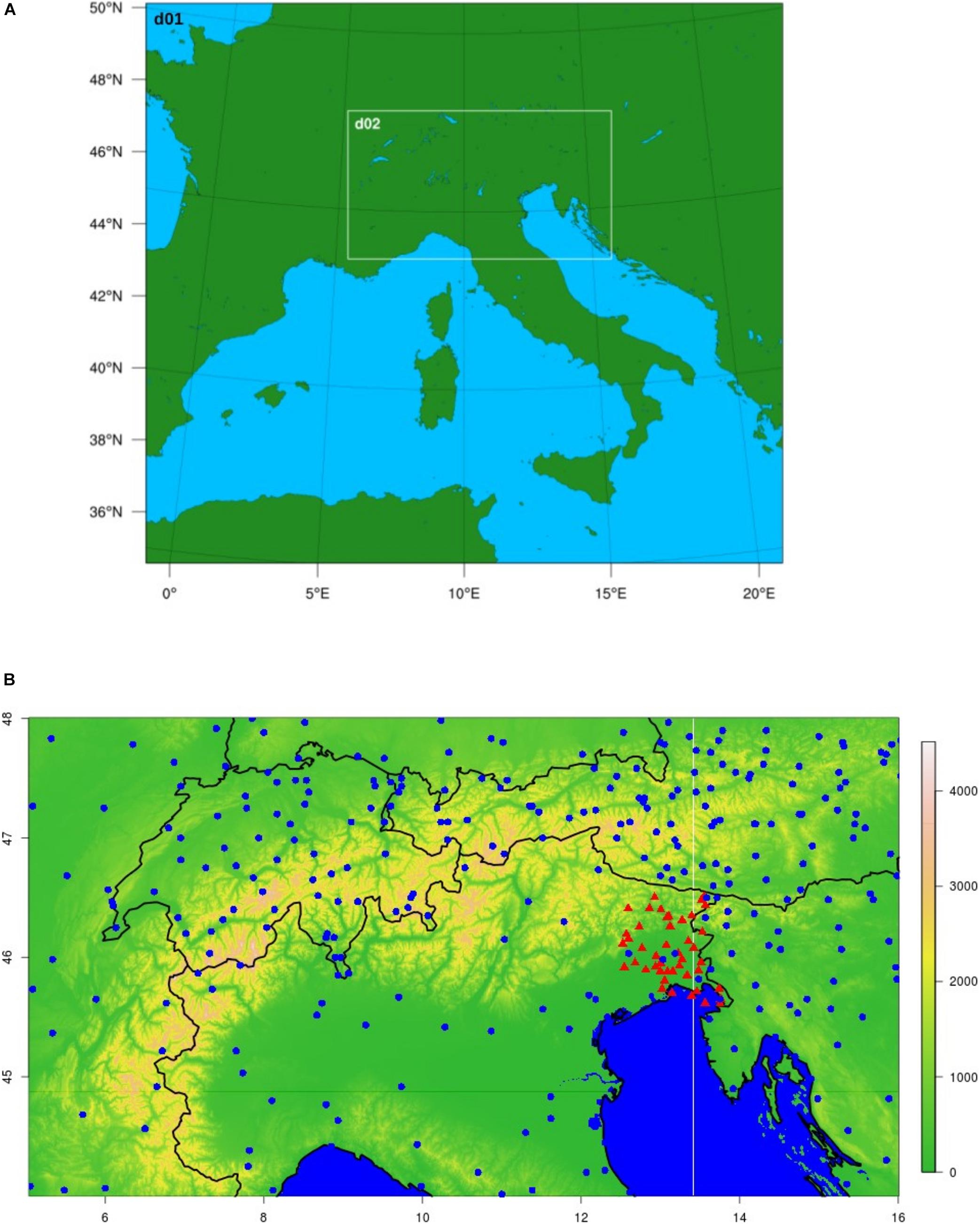
Figure 1. The static domains d01 and d02 used to perform the WRFBG simulations [(A), top]; geographical distribution [(B), bottom] of the available METAR stations (blue circles) and the OSMER stations (red triangles).

WRF

The Weather Research and Forecasting (WRF) model is a non-hydrostatic mesoscale numerical weather system (Skamarock et al., 2008). It has been developed mainly at the National Center for Atmospheric Research (NCAR), in collaboration with the National Oceanic and Atmospheric Administration (NOAA) and other research institutes. The horizontal domain can be selected among different projections (polar stereographic, Mercator and Conical Lambert conformal). In the present set of experiments, the Conical Lambert Projection has been chosen with the tangent option.

For each case study reported in Table 1, the survey time of the retrieval of the SAR wind determines the time of the LAPS analysis, which is used as initial condition for the WRF model simulations. The twenty selected case studies cover a wide range of atmospheric scenarios, including episodes characterized by flow over complex orography (Jiménez and Dudhia, 2012, 2013; Gómez-Navarro et al., 2015) conducive to episodes of orographic convection, which occasionally occur in this area (e.g., Manzato et al., 2020). The numerical experiments are performed over the geographical domain shown in Figure 1A, using a two-domain one-way-nested configuration, where d01 and d02 are the external and internal domain, respectively. Table 2 specifies the features of the static domain for the experiments, the time steps and the duration of the model runs. Figure 2 shows the methodology adopted to implement the WRFBG and WRFHR runs, as explained in the following subsections.

TABLE 2

Table 2. Set up for the WRF model simulations and parameterization schemes.

FIGURE 2

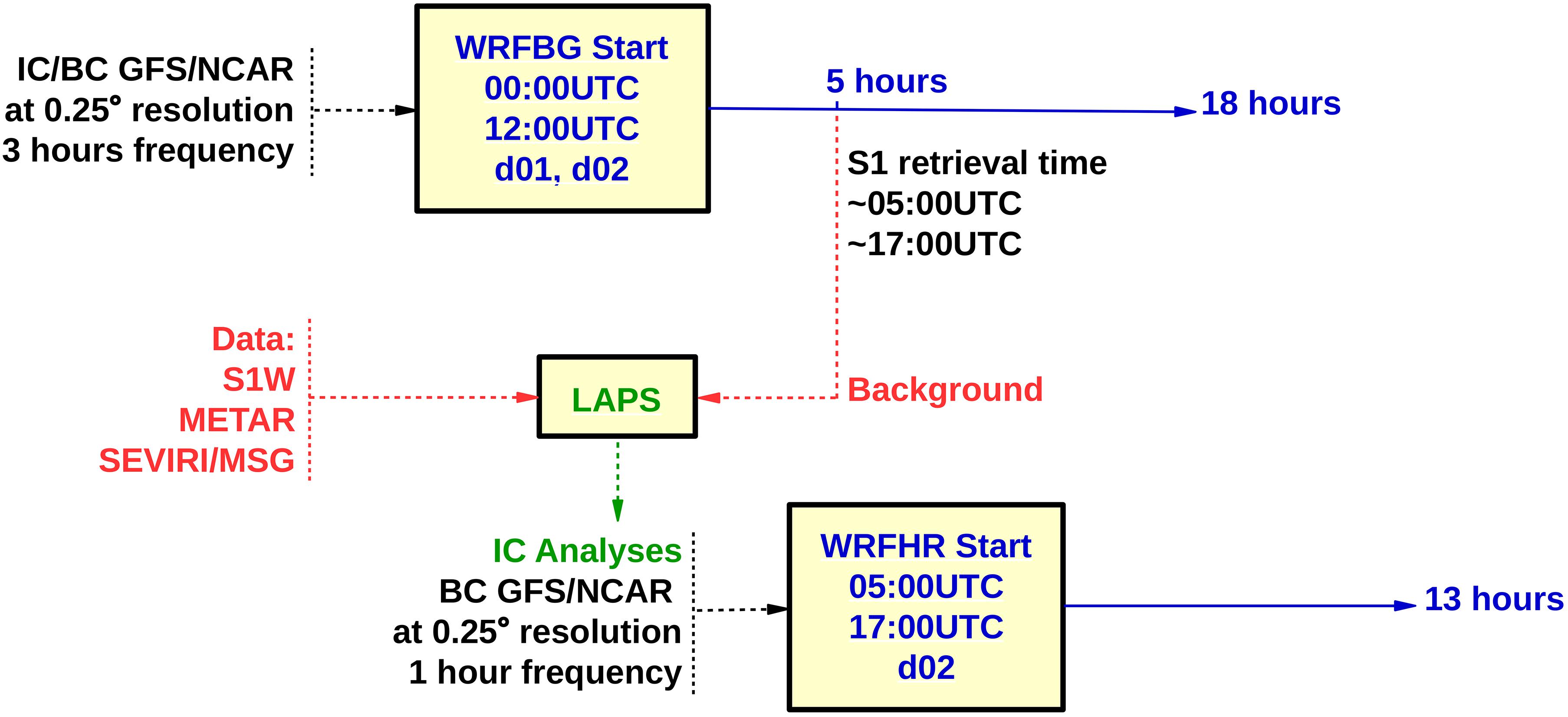
Figure 2. Framework set up for the simulations of the case studies with the LAPS-WRF modeling system.

WRFBG

A WRF model simulation (WRFBG) provides the background fields for the LAPS analyses. Figure 1A shows the two one-one-way domains. IC and BC are provided by the Global Forecast System (GFS) analysis and forecasts, respectively, at the resolution of 0.25°, available at the website https://www.ncdn.noaa.gov/; BC are provided at 3-h intervals. Because of the times of S1 retrieval over the northern Adriatic Sea (i.e., 05:00 UTC and 17:00 UTC), the starting time of each experiment is set consequently: for a morning survey of S1, the WRFBG simulation starts at 00:00 UTC; for an evening survey, the WRFBG simulation starts at 12:00 UTC, so that the background fields in which the Sentinel-1 data are ingested are obtained after 5 h of spin-up time. Table 1 reports the WRFBG start time for each case study.

WRFHR

High-resolution WRF (WRFHR) experiments are performed over the inner domain d02 shown in Figure 1A. The complete set up of WRFHR runs is listed in Table 2, and Figure 2 depicts the way these simulations are implemented. The starting time of each simulation is the approximate survey time of the S1 retrieval: 05:00 UTC for the morning retrieval and 17:00 UTC for the evening retrieval. The WRFHR simulation IC consists of the analyses provided by LAPS, while the BC are provided hourly and are the time interpolations of the GFS forecasts, provided at 3-h intervals. The initialization of the WRFHR simulations is performed in “hot start” mode, which means that the IC include microphysical species, as provided by the LAPS analyses (the proper treatment of the microphysical species in LAPS requires the SEVIRI/MSG data as input). The analysis procedure performed with LAPS is described in detail in the following subsection “LAPS Implementation.”

Such a method cannot be considered as proper data assimilation but rather falls into the initialization category, since it does not correct boundary conditions or model dynamics as the integration proceeds further in time. Depending on the model domain size, this may cause a quick deterioration of the solution after boundary conditions dominate the solution (and quickly sweep the initial state). For these reasons, simulations have been evaluated only in a limited temporal range (0–13 h), when boundary conditions are supposed not to dominate the solution yet.

LAPS Implementation

The Local Area and Prediction System (LAPS) has been developed at NOAA to generate analyses for purposes of nowcasting and assimilation of meteorological data into numerical models (McGinley et al., 1992; Albers et al., 1996). It performs the ingestion and the assimilation of virtually any kind of data (conventional and non-conventional) based on the recursive Barnes scheme (Barnes, 1964). More recent versions of LAPS are migrating toward a variational approach with the perspective of application of the Ensemble Kalman filter (EnKF) (Xie et al., 2011; Toth et al., 2014; Jiang et al., 2015). Compared to more advanced and complex methods - for instance, variational approaches such as the 3DVAR/4DVAR (Lorenc, 1986; Courtier and Talagrand, 1987), EnKF (Evensen, 1994; Tippett et al., 2003; Ott et al., 2004), or hybrid 3DVAR/4DVAR (Hamill and Snyder, 2000), one of the greatest advantages of LAPS is the high adaptability to different computer architectures without requiring large computational resources, which made LAPS a very competitive tool for nowcasting and for short range weather forecasting also in operational environments. Barcons et al. (2015) compared the initialization of WRF through LAPS and WRFDA, showing that the Barnes analyses produced by LAPS are at least as adequate as those obtained with 3DVAR for model initialization.

The setup of LAPS simulations consists of two different stages: first, the ingestion of the background fields (e.g., WRFBG) and the observational data; second, sequential modules perform the analysis of the winds (2D and 3D), of all surface fields, and 3D analyses of temperature, moisture, ice and water cloud content. Finally, an interface module collects and arrange the analyzed fields into the format required for the initialization of a WRF (WRFHR) run. The modules are based on different approaches: in the early versions, analyses are based on the recursive Barnes scheme (Barnes, 1964). The implementation used in this paper is the result of several years of activity performed at the National Research Council of Italy, Institute of Atmospheric Sciences and Climate (CNR-ISAC), including the ingestion of the Spinning Enhanced Visible and Infrared Imager/Meteosat Second Generation (SEVIRI/MSG, Eumetsat; Conte et al., 2010, 2011). The development of LAPS is performed in close collaboration with the NOAA developers and other European institutions (Barcons et al., 2015; Gregow et al., 2015; Tiesi et al., 2016). In the present article, the focus is on the impact of the S1 SSW data on model simulations; for these reasons, the data ingested into LAPS in the present work are limited to:

• The Brightness Temperature of the infrared channel at 10.8 μm (BT11), obtained from the radiances sensed by SEVIRI/MSG; these data are necessary to produce the 3D cloud analysis and to set up the microphysical species necessary to initialize WRF in “hot start” mode;

• Data from the METAR network. These surface data have been ingested in several model runs either alone or together with S1W in order to assess the contribution of S1 wind in the simulations. Figure 1B shows the METAR station locations (blue circles); the 77 METAR stations used for the initialization belong to the d02 domain.

• S1 SSW data. These data are expected to provide an important contribution to the model in describing local wind patterns over the sea, where the presence of in situ data is limited.

Other sources of data have been exploited at CNR-ISAC in the past, e.g., radiosoundings, and radar reflectivity (CAPPI 3 levels) provided by the Italian Civil Protection Department, but the analysis of their contribution is out of the scope of the present work, since the goal here is to single out and assess the impact of the ingestion of S1 SSW.

Preprocessing of the S1 SSW and Interface With LAPS

The pixel resolution of the SAR wind data provided by DTU is 500 m. For every grid point, the corresponding wind direction is originally taken from the global model GFS at the nearest primary synoptic time (00:00, 06:00, 12:00, and 18:00 UTC). In the implementation used for the case studies of Table 1, the GFS wind direction is not considered and the ingestion is limited to the SSW intensity only, leaving unaltered the WRFBG wind direction due to its better resolution compared to the GFS; this should allow a better representation of the smallest scale wind patterns, which may be missed by the global model.

The satellite wind data are ingested as they were observed at a surface station over land (the radius of influence of the data, to be defined in LAPS, is set to 10 km). A procedure has been defined to ingest the S1 SSW into the LAPS system, in the following steps:

• Verify that the retrieved data corresponds to sea in the model land mask and are inside the d02 domain (Figure 1B);

• Degrade the data resolution from 500 m to 2 km (model grid spacing) by adopting the nearest-neighbor grid point approach in the model grid;

• Write the wind data in a format compliant with the LAPS ingestion routines.

After the S1 wind is ingested into LAPS (at 05:00 or at 17:00 UTC), the LAPS analysis is used to initialize a WRFHR simulation covering the following 13 h (respectively, until 18:00 UTC for a morning start, 06:00 UTC of the following day for an evening start).

Selection of the Case Studies

The case studies shown in Table 1 are selected among those retrieved, and characterized by at least one of the following features:

• Heavy precipitation (the precipitation event occurs mainly within 3–9 h after the S1 retrieval time);

• Hailstorms;

• Bora wind, which is a typical north-easterly wind occurring in the Adriatic Sea (Horvath et al., 2009).

The retrieved SAR wind should cover at best the whole Northern Adriatic basin in order to avoid discontinuities in the analysis, associated with sharp edges in the sea surface wind. The selection of the case studies depends on the data availability: the S1 lies on a polar orbit whose revisiting time of 12 days ruled out the study of many relevant episodes.

OSMER Data

Surface data, used for the sake of comparison with the model simulations, were retrieved from sixty-three stations of the Friuli Venezia Giulia network, hold by the Regional Department of Civil Protection and built by SIAP-MICROS and CAE companies. The data are collected and checked by the Regional Agency for the Environmental Protection of Friuli Venezia Giulia - Regional Meteorological Observatory (ARPA-FVG - OSMER). The dataset is composed by measurements sampled every one minute and then aggregated into hourly data. The geographical distribution of the sixty-three WMO-compliant regional stations is shown in Figure 1B (red triangles). The Friuli Venezia Giulia area ranges from the eastern Alps to the northern Adriatic coast, through the northeastern Po Valley. Thus, the wind features in the northern Adriatic are relevant for the weather in the region.

METAR Data

A set of available METAR data was downloaded from the website https://www.wunderground.com/; the METAR stations for the initialization task, which fall into the d02 domain are 77. Figure 1B shows the geographical distribution of the available METAR stations as blue circles. METAR data are used both for the initialization of some WRFHR experiments and the verification of model simulations.

Results

The WRF simulations (WRFBG and WRFHR) are compared with the OSMER and METAR surface stations. The METAR observations ingested into LAPS are taken at the initial time, while those at later times are used for comparison. For each case study summarized in Table 1, the WRF model simulations were performed using the setup shown in Figure 2 using the following four configurations:

• WRFBG: The background configuration over the two domains d01 and d02 (Figure 1A); the simulations cover 18 h (the first 5 h are considered as spin up time) for each of the 20 case studies listed in Table 1.

• WRFHR: Three simulations covering 13 h after the initialization time (i.e., the time at which the S1 SSW data are retrieved); in particular, the following configurations are considered:

• HR1: initialized with BT11 and S1 SSW;

• HR2: initialized with BT11 and METAR data;

• HR3: initialized with BT11, METAR data, and the S1 SSW.

Thus, a total of 80 WRFHR experiments was performed for the 20 case studies. In order to allow WRFHR hot start initialization, the analyses must include BT11 to ensure the inclusion of the microphysics variables. The performance of the simulations is summarized using statistical indices – see Appendix and Wilks (2011) for their definition -, like BIAS and Root Mean Square Error (RMSE) for surface wind speed WS and wind direction WD, temperature T2M, and dew point temperature TD2M (Figures 3, 4). Furthermore, Taylor diagrams are shown to summarize global performances (Taylor, 2001) of the four sets of WRF runs: each one is evaluated for 13 h after the time of the S1 retrieval (Figures 5, 6). A geographical distribution of BIAS and RMSE (in comparison with the OSMER records) is also shown (Figure 7).

FIGURE 3

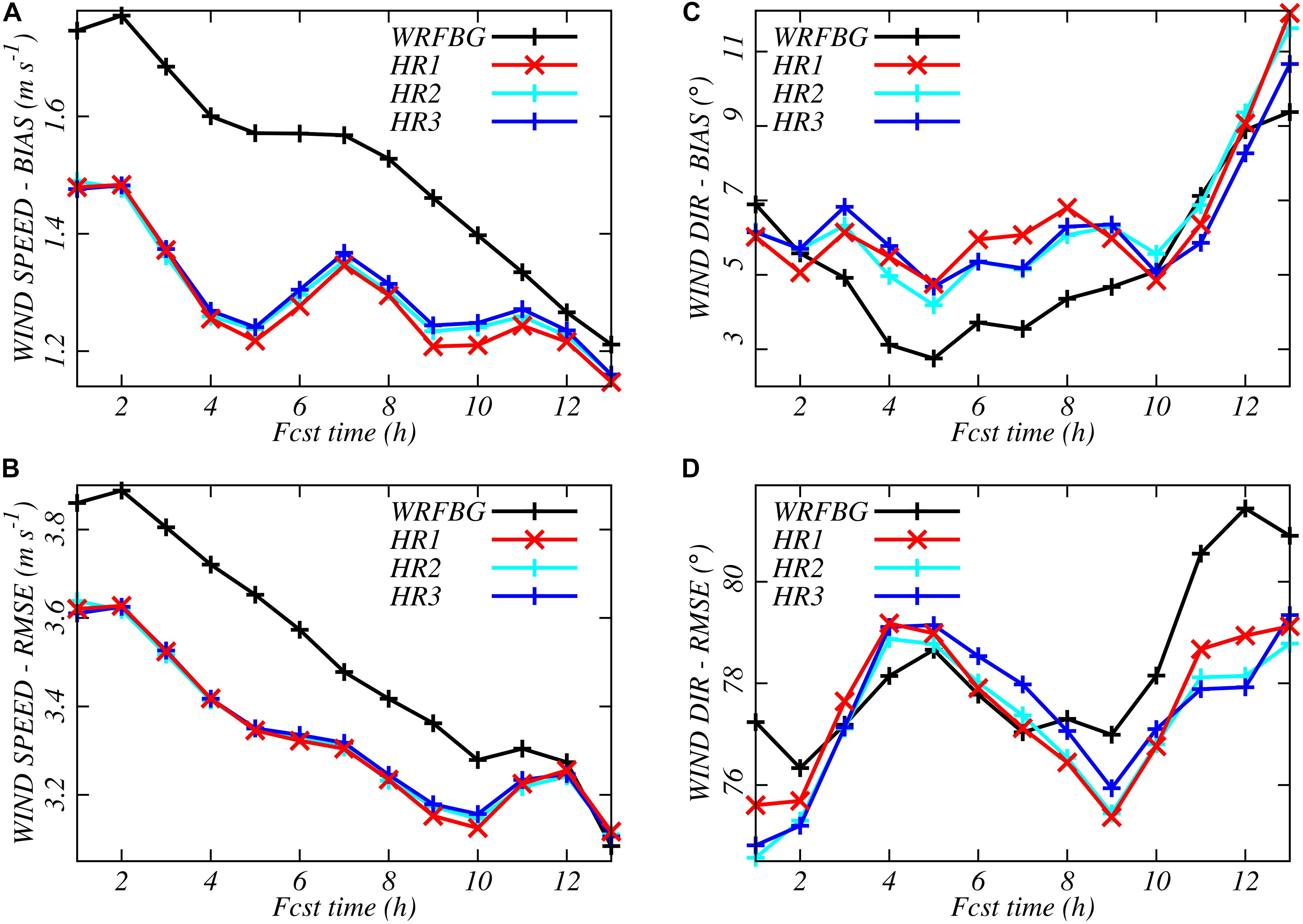
Figure 3. 10 m wind speed BIAS (A) and RMSE (B), and 10 m wind direction BIAS (C) and RMSE (D) for the whole set of case studies as a function of the simulation time. The hourly values of the indices, based on the output of the reference simulation WRFBG, are represented in black, HR1 (initialized with MSG and S1W) in red, HR2 (initialized with MSG and METAR) in cyan, and HR3 (initialized with MSG, METAR, and S1W) in blue.

FIGURE 4

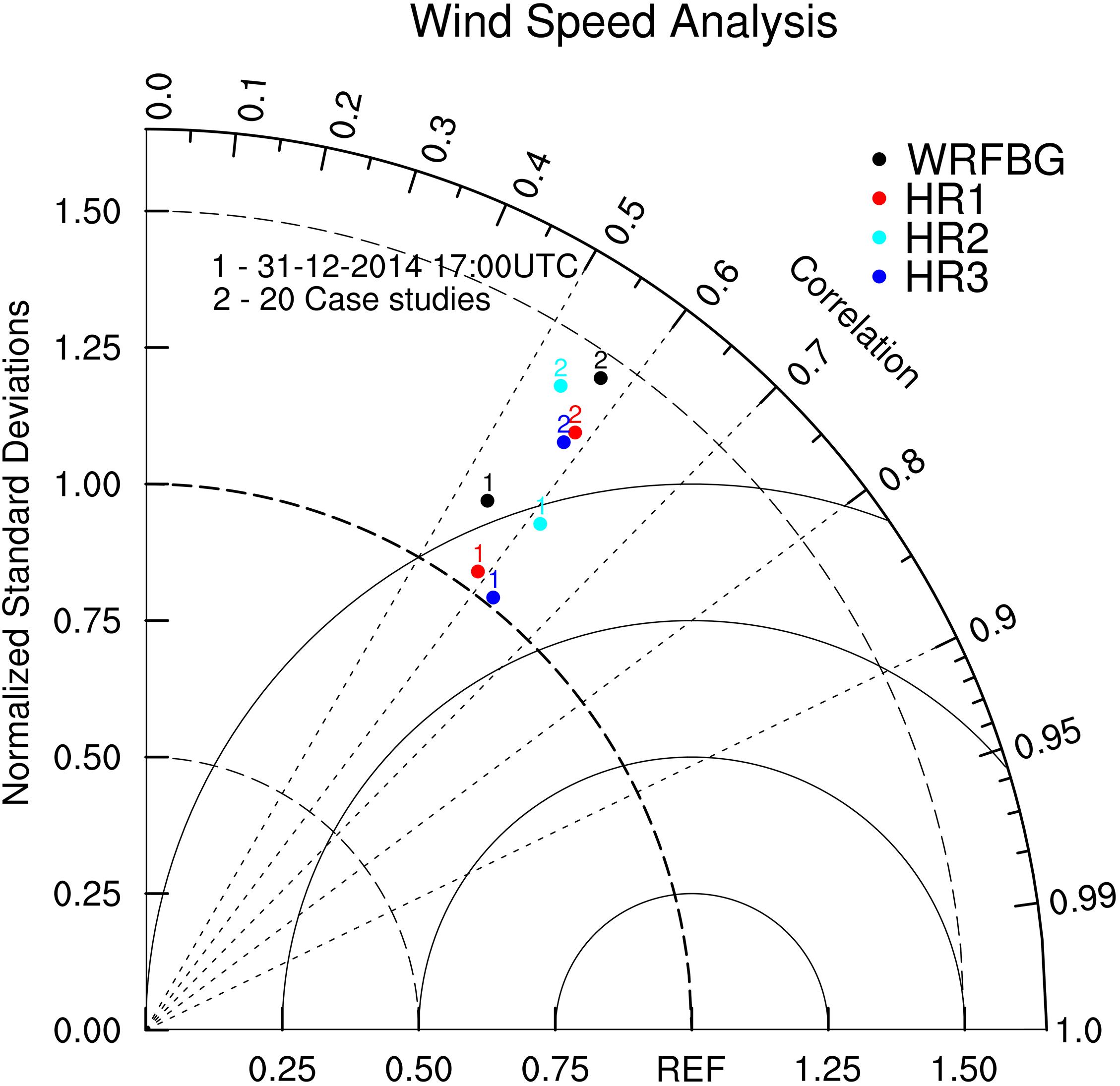
Figure 4. Taylor diagram for the analysis of wind speed for the case of 31 December 2014 (Bora case) and for the 20 case studies analyzed in north-eastern Italy.

FIGURE 5

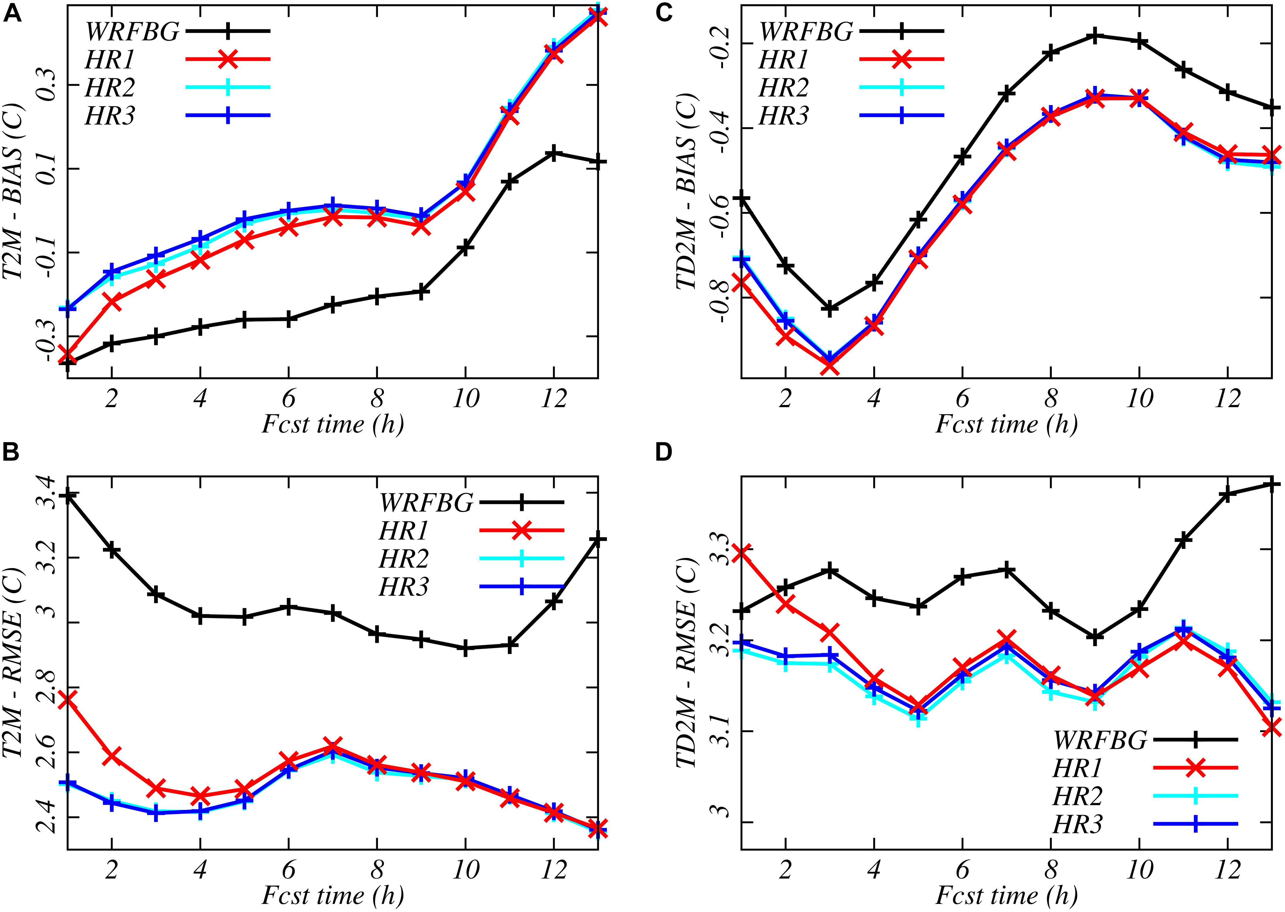
Figure 5. 2 m temperature BIAS (A) and RMSE (B), and 2 m dew point temperature BIAS (C) and RMSE (D) for the whole set of case studies versus the forecast time. Colors as in Figure 3.

FIGURE 6

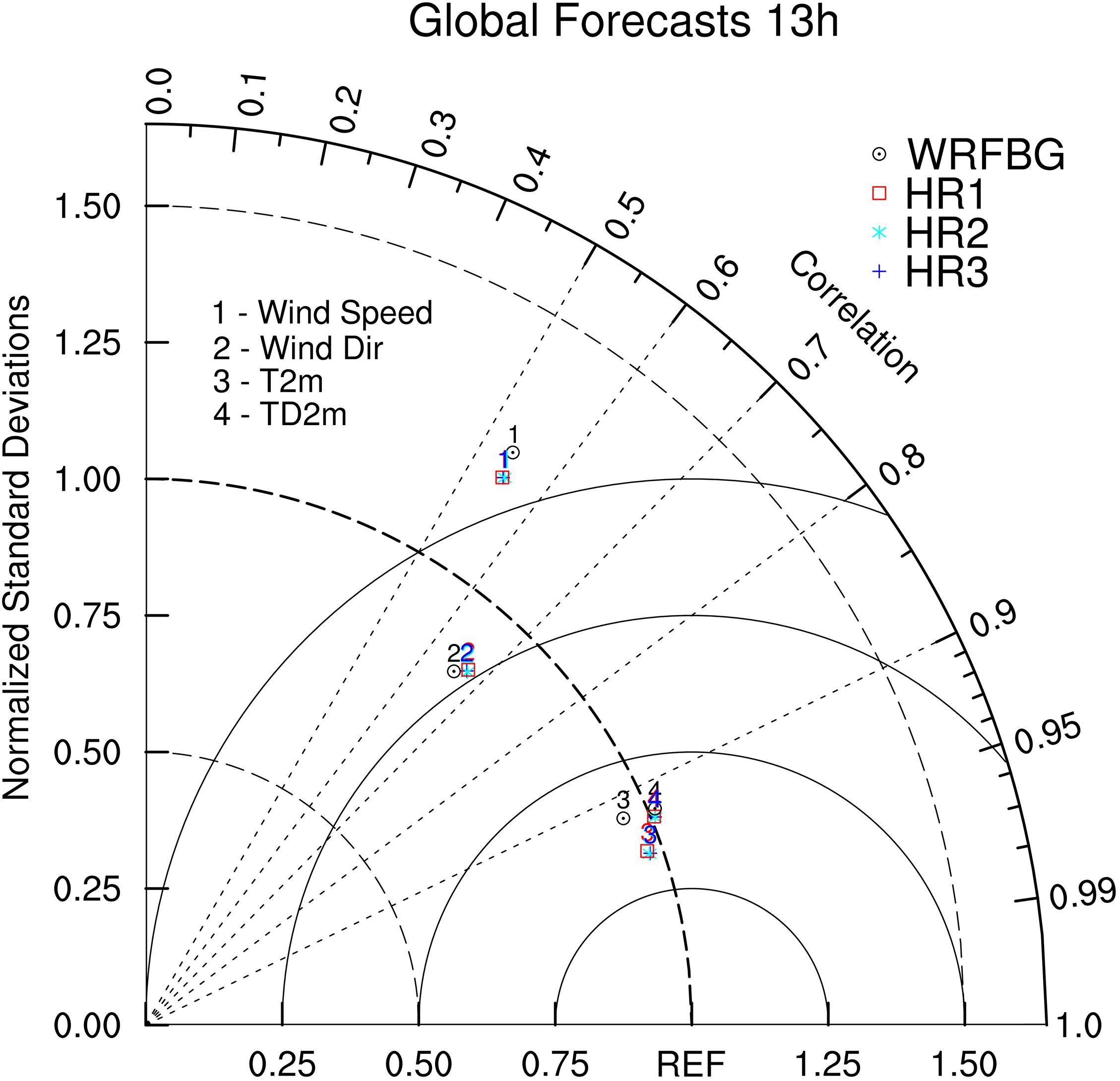
Figure 6. Taylor diagram for the simulations. The data refer to the complete set of case studies in all the 13 h after the retrieval of S1 (in the simulation range 1–13 h for the WRFHR runs and in the range 6–19 h for the WRFBG run).

FIGURE 7

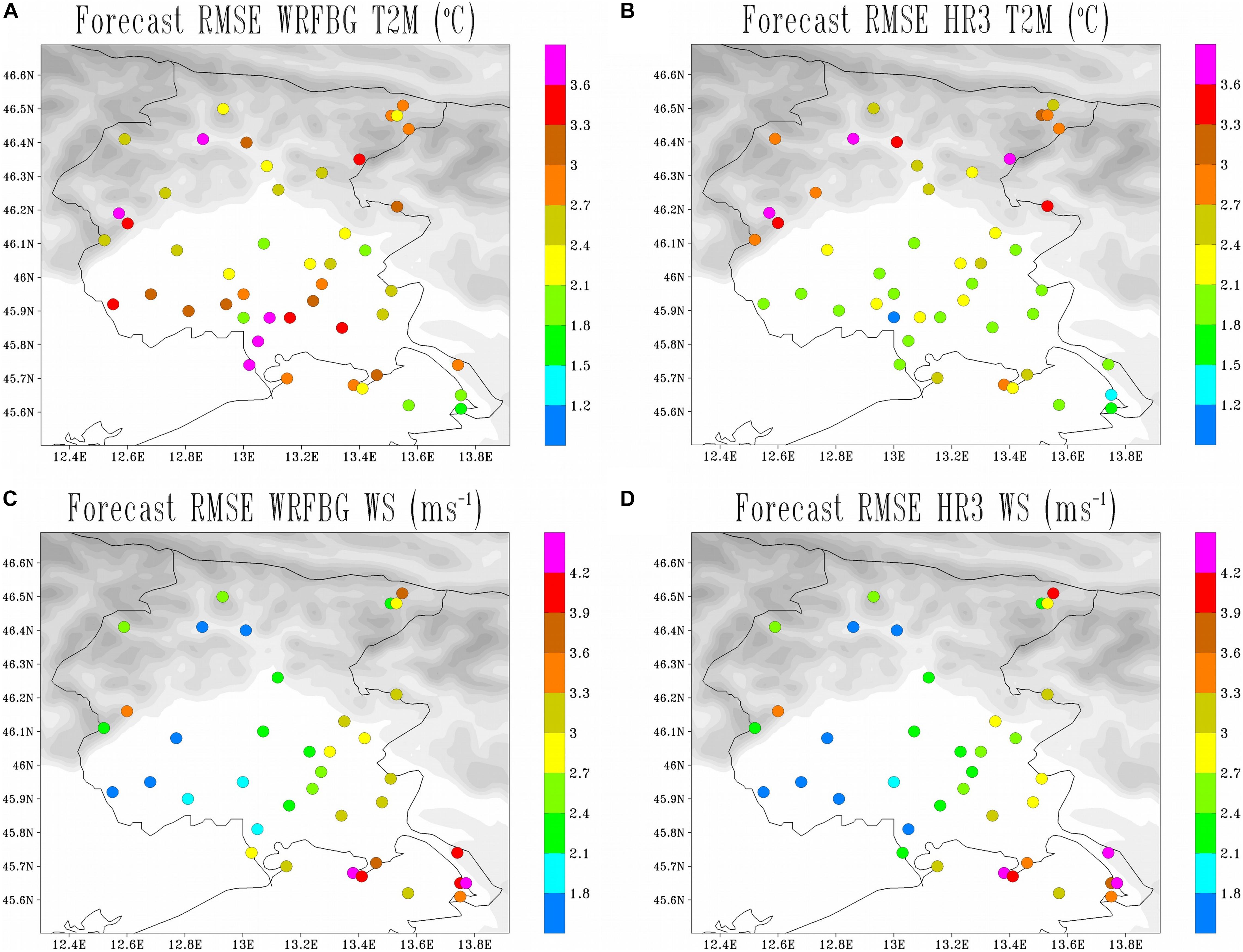
Figure 7. Geographical distribution of RMSE for T2M (top) in the WRFBG run (A) and in the HR3 run (B), and wind speed (bottom) in the WRFBG run (C) and in the HR3 run (D).

Ingestion of the SAR Wind

The initialization using the S1 SSW is expected to have an impact on model simulations, due to a better and finer representation of the low-level wind, which is only roughly represented in large-scale analysis. The higher resolution of the S1W field helps to better represent the local scale features in the open sea and near the coasts, where the land-sea border makes the representation of wind more critical. Furthermore, the wide sea sectors covered by the S1 SSW data can improve the representation of the regional circulation at the initial time and consequently affect the simulation of the other meteorological variables at later times too.

A quantitative assessment of the impact of the data ingestion on the 10 m wind field analysis is summarized in the Taylor diagram (Taylor, 2001) in Figure 5. The comparison is performed with the independent set of data from OSMER meso-network. Compared with the WRFBG run, an improvement can be noted both in correlation, normalized standard deviations, and centered RMSE, in particular for the analyses ingesting the S1 wind (HR1 and HR3 runs).

Impact of the S1 SSW on the Model Simulations

A quantitative verification for the whole set of simulations (WRFBG and WRFHR) is performed through BIAS and RMSE in 140 surface station (77 METAR and 63 OSMER stations). As discussed above, the HR1 (HR2) experiment results take into account the impact of S1 SSW (METAR) on the model simulations (see also Barcons et al., 2015; Tiesi et al., 2016). METAR surface wind and S1 SSW are ingested into LAPS assuming identical weights and influence radii; anyway, for future applications it should be necessary to test other strategies for these datasets due to the different sampling and retrieval approaches. Finally, HR3 statistics are also reported to evaluate the advantage of a combined ingestion of S1 SSW and METAR data in the analyses. In total, 77 METAR are used for the analyses but sometimes they are not available simultaneously, while S1 SSW corresponds to a number of data points ranging between 4,597 and 7,744, depending on the retrieval. In Figures 3, 4, BIAS and RMSE are shown as a function of the simulation time, from the first hour of simulation for the following 12 h.

Wind Speed

Figures 3A,B shows, respectively, the wind speed BIAS and RMSE for the whole set of experiments. The set of WRFHR runs performs better than WRFBG; among the WRFHR runs, the best BIAS (Figure 3A) and RMSE (Figure 3B) is that of HR1; however, the differences among the three WRFHR experiments remain confined within 0.1 m/s. Near the end of the simulation, the difference in RMSE between WRFBG and the WRFHR runs becomes negligible, demonstrating that the positive impact of the LAPS analysis in the initialization of the model progressively reduces and finally disappears after about 12 h. These results are confirmed in Table 3, which reports the BIAS and RMSE relative to wind speed, averaged over the whole duration of the simulation, along with the number of data points involved in the calculation. The results relative to the HR3 run suggest that the inclusion of different sources of surface data does not always guarantee an improvement in the model simulation with respect to the ingestion of a single set of data, thus suggesting that possibly different strategies (e.g., different radii of influence) should be tried for different categories of data.

TABLE 3

Table 3. Time averages of the BIAS and RMSE for the whole set of experiments listed in Table 1, calculated over the simulation time interval.

Wind Direction

WD over sea surface is taken from the WRFBG field (while WS is modified by the S1 SSW); inland, the background field is locally modified by the surface station wind data. Following this approach, WS and WD are coherent over all the domain only for the WRFBG run, while in WRFHR runs patterns of wind direction and wind speed may be not consistent over the sea. This explains why the ingestion of surface data does not improve this field in the WRFHR runs. Anyway, for the sake of completeness, Table 3 and Figures 3C,D show the BIAS and the RMSE relative to WD for the whole set of experiments. Overall, the data analysis does not show any improvement in WRFHR runs compared to WRFBG for wind direction.

2 m Temperature and Dew Point Temperature

Figures 4A,B shows, respectively, the BIAS and RMSE of 2 m temperature T2M for the whole set of experiments. Figure 4A shows that, in the first 9 h of simulation, an underestimation is present in WRFBG, which is reduced in the WRFHR experiments. The HR1 experiments show a limited improvement in the initial part of the model simulations compared to the HR2 and HR3 runs, due to the fact that the METAR data (ingested in the latter runs) modify T2M at the initial time in the verification points, while the HR1 initialization includes modifications only in wind speed over the open sea, thus far from the verification points, and no corrections to T2M. Table 3 shows the positive impact on T2M due to the ingestion of surface data.

Figure 4B shows a general improvement in RMSE for the WRFHR experiments compared to WRFBG. The HR1 run shows a higher RMSE than HR2 and HR3 in the first few hours, but, as in Figure 4A, after 9 h the differences among the WRFHR experiments become negligible. Table 3 confirms the positive impact of data ingestion on the model forecast of T2M in terms of RMSE, since, in all WRFHR experiments, RMSE is smaller by more than 0.5°C compared to the WRFBG runs.

Figures 4C,D shows the BIAS and the RMSE of TD2M. In terms of BIAS, the WRFBG run performs better than the WRFHR runs. Conversely, Figure 4D demonstrate a slight positive impact of data ingestion on RMSE, as also reported in Table 3.

Figure 6 shows the Taylor diagram summarizing the performance of the whole set of simulations in comparison with both the datasets available (METAR and OSMER). The data refer to the complete set of case studies in the 13-h time window after the retrieval of S1 (in the simulation range 1–13 h for the WRFHR runs and in the range 6–19 h for the WRFBG run). The data ingestion produces a general improvement in WRFHR runs for all fields, especially for wind speed (in terms of normalized standard deviation) and T2M (in terms of correlation).

In order to analyze where the data ingestion improved the simulation results, Figure 7 show the geographical distribution of RMSE in correspondence of the OSMER surface stations for WRFBG run (left) and HR3 (right), for T2M (top), and for WS (bottom). An improvement in T2M is observed in HR3 run, mainly in the stations in Po Valley and along the coast, while in the Alpine area WRFBG performs slightly better (Figures 7A,B). For wind speed, the improvement regards mainly the stations in the Po Valley, while the RMSE remains nearly unchanged for the mountain and coastal stations. It is remarkable that, for all runs, the highest RMSE for wind speed is observed in the stations along the coast; our interpretation is that the irregular coastline combined with the proximity of the mountains near the east coast make the local circulation very complex, due to the combination of sea and mountain effects that are difficult to simulate properly.

Discussion

To analyze the generality of our statistical results, we compare the BIAS and RMSE obtained for the reference WRFBG run with those reported in similar studies in literature. Jiménez and Dudhia (2012) performed a numerical study concerning the simulation of 10 m wind speed over a domain covering the Ebro river valley, between the western Pyrenees and the Iberian system. The study showed, in a region with complex topography, an average underestimation of surface winds over peaks and hills and an overestimation in valleys and lowlands. Jiménez and Dudhia (2013) performed in the same region an analysis of the WRF skill for the simulation of wind direction, finding a RMSE greater than 70° for complex terrain, which is comparable with the values of RMSE reported in Table 3.

Gómez-Navarro et al. (2015) performed a sensitivity study of 10 m wind simulated with the WRF model for different parameterizations of the Planetary Boundary Layer (PBL) in the Alpine region, comparing the surface winds with the Meteo Swiss network of meteorological stations for a set of 24 historical windstorms. The BIAS and RMSE in section “Impact of the S1 SSW on the Model Simulations” show comparable or slightly better values compared to those presented in Gómez-Navarro et al. (2015) for the same PBL parameterization and 2 km grid spacing.

Barcons et al. (2015) performed experiments in 29 case studies, initializing WRF with either LAPS or WRFDA. They found that, using a grid spacing of 1 km, the LAPS initialization performs better than WRFDA due to its ability to better represent high density surface data on the high-resolution grid, obtaining values of RMSE slightly better than in our study. The latter result can be possibly attributed to the higher resolution adopted in their experiments.

Avolio et al. (2017) explored several PBL parameterizations in WRF for a set of case studies over the southern Italian region of Calabria, which presents a complex morphology due to the presence of a rough orography in a narrow peninsula. They obtained comparable or slightly better RMSE than in our runs. Tiesi et al. (2018) applied the same LAPS-WRF system employed here to a domain similar to that used in Avolio et al. (2017), performing 1 year of short-range forecasts, obtaining similar results to the latter study. This demonstrates that the system implemented in the present work can perform in a way similar to other studies reported in literature in areas with complex morphology, and the differences in the statistical indices with the present work are mainly determined by the different, rougher topography of the Alpine region, and of the Friuli Venezia Giulia region in particular.

A result emerging from the numerical simulations is that they tend to lose predictability very rapidly. This is clearly shown in Figure 3 where the advantage of using a smart initialization with LAPS analyses is lost after 12 h for the simulation of wind speed. This is not an unexpected result. Daley (1991) discusses vertical correlation functions computed between the geopotential background error at 400 hPa and that at other levels. Clearly, an observation at 400 hPa will receive a good weight for the analysis of geopotential at the same level, but it will have a slightly smaller weight for the analysis at 500 or 300 hPa, and correlation will become very small with a level near the surface, so the latter observation would influence the upper analysis only a little. In fact, an observation at the surface will mainly affect levels below 500 hPa, and will have only little influence in the upper troposphere. This is a consequence of the planetary boundary layer, which confines the influence of the observations to lower levels. Consequently, although the vast majority of in situ observations are taken at the surface, they provide only a limited impact in the upper troposphere.

As the model integrates further in time, the initial improvements are progressively lost, since the method used here does not correct both boundary conditions, which originate solely from the global atmospheric model, and model dynamics, as it is done, for example, in nudging methods (Stauffer and Seaman, 1990). The limited size of the inner model domain (d02 in Figure 1A), where observations are ingested into the analysis, can cause a quick deterioration of the solution after some hours, as boundary conditions start to dominate the solution and rapidly sweep the initial state. In order to improve the simulations over a longer time interval, one should consider the setup of a larger domain, especially on the eastern and southern side, considering that many cases analyzed in the present paper refer to systems moving from the eastern/southern boundaries (Bora-Sirocco in the Northern Adriatic Sea; Table 1), which are very close to the studied area. As an example of the latter category of events, Figure 8A shows the S1 SSW retrieval at 16:58 UTC, 31 December 2014, during a typical northern Adriatic northeasterly wind (Bora) episode. The ingestion of the S1 SSW affects the background 10 m wind, reshaping the wind patterns in the initial conditions for HR1 (and HR3) run and producing a more realistic wind field compared to WRFBG (cfr. Figures 8B,C with Figure 8A). The improvement in the wind speed analysis in this case is significant for HR1 and HR3 both in terms of correlation, normalized standard deviations, and centered RMSE.

FIGURE 8

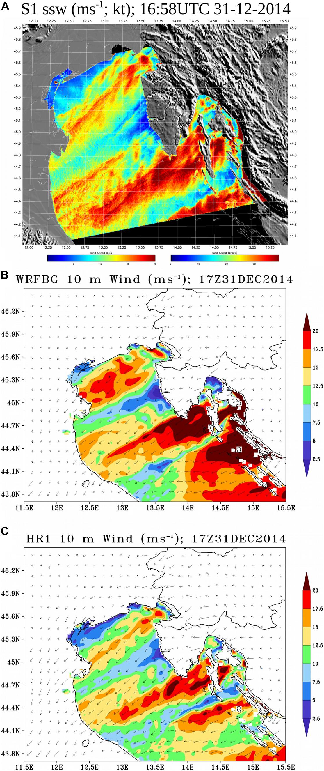
Figure 8. (A) S1 retrievals of SSW on 31 December 2014 at 16:58 UTC; (B) WRFBG and (C) HR1 10 m wind at 17:00 UTC.

Another relevant aspect of our results is the better performance of the model simulations in the Po valley (Figure 7). Apparently, the plains take a longer “memory” compared to both the coastal and the mountain stations. This is a consequence of the complex morphology of the region considered in the present study. The arc-shaped coastline shows some lagoons on the western side, which produce a complex land-sea mask, only partially resolved by the model grid and represented in the large-scale sea surface temperature used as lower boundary condition. At the same time, the eastern coastal area is affected by a complex combination of sea breeze and mountain flows that interact with each other, due to the proximity of the steep orography. These considerations are valid for the twenty selected case studies, which are often characterized by severe, rapidly evolving weather conditions.

Another interesting aspect emerges in Figure 9, which shows the observed and simulated wind speed distribution (bins of 2 m/s) in all OSMER and METAR stations over all 20 case studies, 6 h after the S1 retrieval time. Comparing the histograms, it is clear that the gray columns (observations) are closer to the colored ones (WRFHR runs) than to the black ones (WRFBG), especially on the left and on the right side of the distribution, suggesting that the estimate of high (above 12 m/s) and very weak wind speeds improves, albeit modestly, with data ingestion. Again, the advantage of data ingestion is reduced when longer simulation time ranges are considered (not shown). Overall, the data ingestion does not improve significantly the simulation results.

FIGURE 9

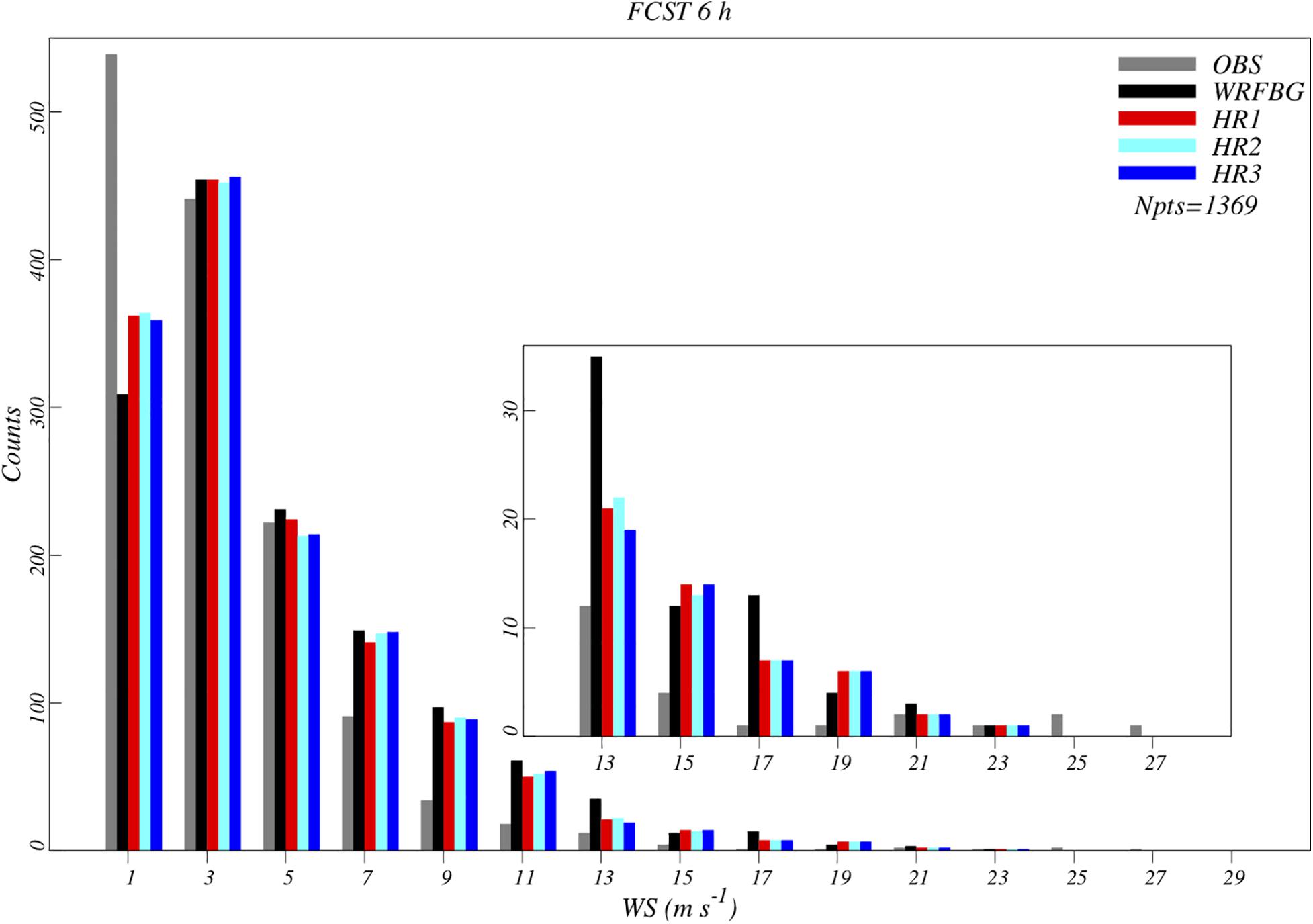
Figure 9. Observed and simulated wind speed distribution (number of events in bins of 2 m/s) in all OSMER and METAR stations over all 20 case studies, 6 h after the S1 SSW retrieval. The inset zooms in on the higher wind speeds (above 12 m/s).

Medicane Case Study: NUMA

In this section, an example of application of model initialization with the S1 SSW to a tropical-like cyclone in the Mediterranean (TLC or Medicanes) is shown. Medicanes are receiving a growing attention in the literature, due to the severity of winds, rainfall, and storm surge induced by these intense cyclones (e.g., Fita and Flaounas, 2018; Miglietta, 2019; Miglietta and Rotunno, 2019). In particular, the predictability of these events has been the subject of several papers, which have shown how the intensity and the location of the simulated cyclones may significantly depend on the large scale forcings (Chaboureau et al., 2012; Di Muzio et al., 2019), on the selected model (Davolio et al., 2009), on the physics parameterizations (Miglietta et al., 2015), on the interaction with ocean features (Ricchi et al., 2017).

The cyclone considered here (known as Numa) developed on 14 November 2017 in the Tyrrhenian Sea around the coasts of Sicily, and reached its maximum intensity above the Ionian Sea, causing twenty-two casualties in Greece and estimated damages for around 100 M€ in Italy and Greece; later it dissipated over the western Turkish coasts on 20 November. The cyclone was described in Marra et al. (2019), where the synoptic environment, the remote sensing detection and numerical simulation are discussed. In the present paper, we focus on the effect of the analysis of the S1 SSW and its impact on the WRF model simulations.

Figures 10A,B show the S1 SSW corresponding to the morning descending survey of the Sentinel-1A platform at 04:47 and 04:48 UTC, respectively, 17 November 2017. The maximum wind speed retrieved by S1 reaches 30.6 m/s, i.e., it is near the lower end of category 1 hurricane intensity in the Saffir-Simpson scale. Hence, such a value largely exceeds the estimation performed by the lower resolution (25 km) ASCAT, the sensor on board the polar MetOp A, equal to 20 m/s (Marra et al., 2019). Thus, Sentinel-1 can represent much better this type of events, which spend most of their lifetime over the sea, providing a picture of the wind around the cyclone eye with an unprecedent detail and accuracy.

FIGURE 10

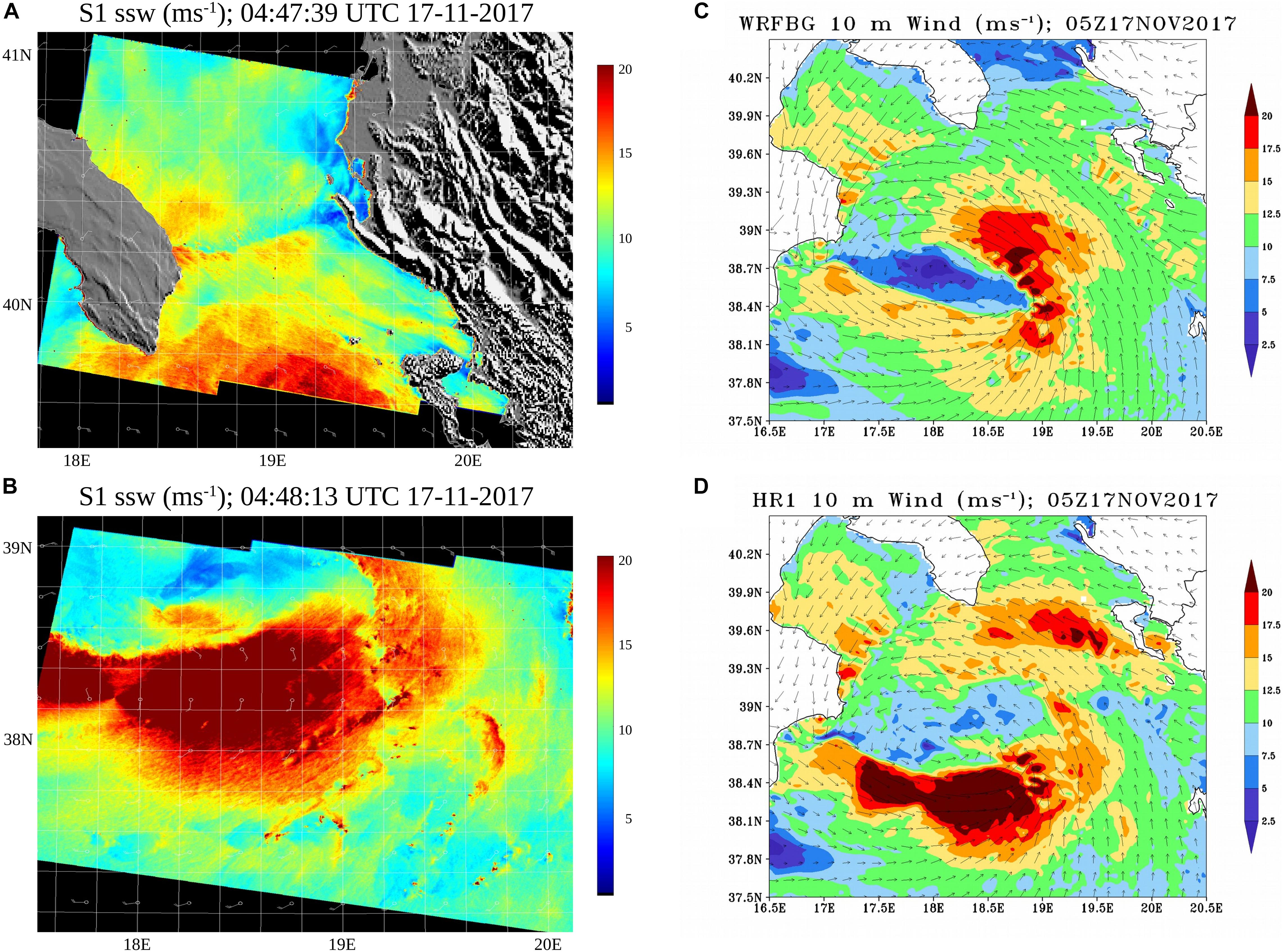
Figure 10. S1 retrievals of SSW on 17 November 2017 at: (A) 04:47, and (B) 04:48 UTC; 10 m wind at 05:00 UTC of 17 November 2017 in: (C) WRFBG run, and (D) LAPS analysis used to initialize the WRFH4 experiment.

Experiment Set Up

The procedure performed to assess the effective impact of the S1 SSW on the WRF model simulations follows the framework introduced in Figure 2. The survey time of the polar platform, 04:48 UTC, is the same as the north Adriatic case studies described in Table 1. For NUMA simulations, the details of two nested domains d01 and d02 are provided in Table 2. Compared to the north Adriatic case studies, the external domain remains the same, the d02 domain resolution remains identical, while the only changes concern the d02 position (centered in the Ionian Sea) and number of grid points, as specified in Table 2. Thus, the reference simulation WRFBG starts at 00:00 UTC, 17 November, while the WRFHR runs start at 05:00 UTC. For NUMA, the nomenclature of the WRF simulations is set as in the following scheme:

• WRFBG: The background configuration over the two domains d01 and d02;

• WRFHR: Two simulations covering 13 h after the initialization time;

• Initialized with BT11, radar reflectivity (CAPPI at 2, 3, and 5 km, provided by the Italian Department of Civil Protection), and METAR;

• WRFH4: as WRFH3, but ingesting also S1 SSW.

Twenty-four METARs were ingested into the LAPS analysis at 05:00 UTC in d02 domain. Interfaces between the DTU product for S1 SSW and LAPS, and analysis settings are identical to those set for the 20 case studies listed in Table 1.

Results: Analysis and Forecast

Figures 10C,D shows the 10 m wind field at 05:00 UTC, respectively, in the reference simulation WRFBG and in the analysis used to initialize WRFH4. The significant changes coming from the ingestion of S1 SSW are apparent over the sea. Indeed, in the southern side of the cyclone eye, where the wind intensity retrieved by the S1 sensor reaches its maximum intensity, the correction to the background field reaches 15 m/s. The comparison between Figures 10C,D highlights the contribution to the SSW in zones with poor data coverage, consequent to the high resolution of S1, as 27382 points are retrieved in correspondence of the d02 domain.

The WRFH4 run reveals an impact of the S1 SSW analysis also on the numerical simulations. Figure 11 shows the time evolution of the distance between the observed center of the cyclone and the minimum SLP for each WRF model realization: WRFBG (black), WRFH3 (green), and WRFH4 (red). The uncertainty in the distance can be estimated as to the sum of the pixel size of the BT11 channel, which is about 4–5 km in the Mediterranean basin, and the model grid spacing, which is 2 km in the model set up. Thus, the total uncertainty in the distance can be assumed to be smaller than 10 km. Figure 11 shows a clear positive impact of the S1 SSW in the simulation of the pressure minimum location by the WRFH4 experiment compared to WRFBG and WRFH3. The improvement occurs at the analysis time and through the first 7 h after the initialization of WRFHR runs. The comparison of the time evolution among the three experiments demonstrates that the S1 SSW can provide a noticeable improvement of the simulation of the cyclone, at least in terms of location (Figure 11).

FIGURE 11

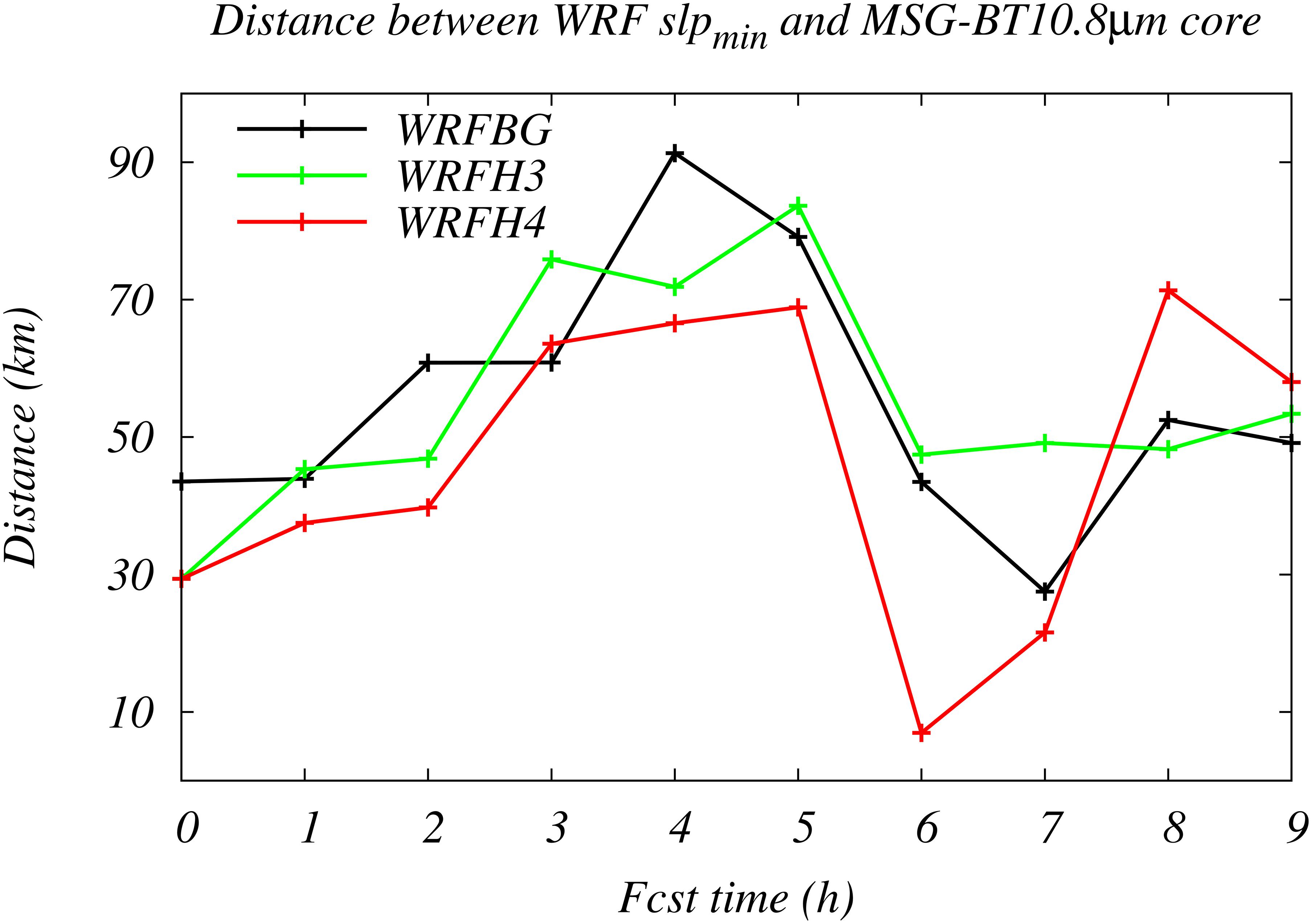
Figure 11. Time evolution of the distance between the simulated minimum SLP and the cyclone eye derived from satellite BT11. The distances are: black for WRFBG, green for WRFH3, and red for WRFH4.

Conclusion

A procedure for the ingestion of Sentinel-1 sea surface wind speed for a smart initialization of the WRF model has been developed. The impact of the S1 wind on the skill of the simulations has been investigated for a set of 20 case studies ranging across different atmospheric scenarios, in order to assess the overall impact, regardless of the specific conditions in each single event. The impact of the data analyses on the model simulations has been described in terms of some statistical scores, comparing the model results with METAR bulletins and surface observations of the OSMER regional network in northeastern Italy.

The results of the verification show a positive, albeit not significant, improvement due to the ingestion of the S1 SSW on the model simulation of surface variables. In this context, the initialization of the WRF model with the S1 SSW is positive, particularly in the first hours of the short-term WRF model simulations, comparable to the impact of METARs. The METAR and S1 data have been ingested assuming identical settings in order to analyze the impact in similar conditions. Analysis through the Taylor diagrams reveals improvement in particular for wind speed and 2 m temperature. The geographical distribution of the RMSE has shown a net positive impact in the Po Valley and a weaker impact for mountain areas and coasts. The improvement is more relevant for high and very small wind speed values.

The ingestion of S1 wind data for the simulation of a Medicane demonstrates their positive impact for severe events over the sea, poorly covered with meteorological data. Such results highlight the important contribution of high quality remotely sensed data in the analysis of the effective state of the atmosphere.

The preliminary results presented here have shown that the impact of S1 SSW on the model positive; the methodology should be consolidated using a larger set of case studies and exploring proper assimilation approaches. The key point of our analysis is that the ingestion of observed sea surface wind provides an improvement in the surface fields, not only over the sea but also over land, and, that the poor data coverage can be enhanced with the help of remotely sensed geophysical quantities.

Data Availability Statement

The raw data supporting the conclusions of this article will be made available by the authors, without undue reservation.

Author Contributions

All authors listed have made a substantial, direct and intellectual contribution to the work, and approved it for publication.

Funding

The authors gratefully acknowledge the funding from the European Commission (Project “CEASELESS,” Grant Agreement No. 730030). AR also gratefully acknowledges the Ministry of University and Research of Italy (PON AIM1858058 – Activity 2–Linea 2.1).

Conflict of Interest

The authors declare that the research was conducted in the absence of any commercial or financial relationships that could be construed as a potential conflict of interest.

References

Ahsbahs, T., Badger, M., Karagali, I., and Larsén, X. G. (2017). Validation of Sentinel-1A SAR coastal wind speeds against scanning LiDAR. Remote Sens. 9:552. doi: 10.3390/rs9060552

CrossRef Full Text | Google Scholar

Albers, S., McGinley, J., Birkenheuer, D., and Smart, J. (1996). The local analysis and prediction system (LAPS): analyses of clouds, precipitation, and temperature. Weather Forecasting 11, 273–287. doi: 10.1175/1520-0434(1996)011<0273:TLAAPS<2.0.CO;2

CrossRef Full Text | Google Scholar

Atlas, R., Hoffman, R. N., Leidner, S. M., Sienkiewicz, J., Yu, T.-W., Bloom, S. C., et al. (2001). The effects of marine winds from scatterometer data on weather analysis and forecasting. Bull. Am. Meteorol. Soc. 82, 437–471. doi: 10.1175/1520-0477(2001)082<1965:TEOMWF>2.3.CO;2

CrossRef Full Text | Google Scholar

Avolio, E., Federico, S., Miglietta, M. M., Lo Feudo, T., Calidonna, C. R., and Sempreviva, A. M. (2017). Sensitivity analysis of WRF model PBL schemes in simulating boundary-layer variables in southern Italy: an experimental campaign. Atmos. Res. 192, 58–71. doi: 10.1016/j.atmosres.2017.04.003

CrossRef Full Text | Google Scholar

Barcons, J., Folch, A., Sairouní Afif, A., and Miró, J. R. (2015). Assimilation of surface AWS using 3DVAR and LAPS and their effects on short-term high-resolution weather forecasts. Atmos. Res. 156, 160–173. doi: 10.1016/j.atmosres.2014.12.019

CrossRef Full Text | Google Scholar

Barker, D. M., Huang, X.-Y., Liu, Z. Q., Auligné, T., Zhang, X., Rugg, S., et al. (2012). The weather research and forecasting model’s community variational/ensemble data assimilation system: WRFDA. Bull. Am. Meteor. Soc. 93, 831–843. doi: 10.1175/BAMS-D-11-00167.1

CrossRef Full Text | Google Scholar

Barnes, S. L. (1964). A technique for maximizing details in numerical weathermap analysis. J. Appl. Meteorol. 3, 396–409. doi: 10.1175/1520-0450(1964)003<0396:ATFMDI>2.0.CO;2

CrossRef Full Text | Google Scholar

Chaboureau, J.-P., Pantillon, F., Lambert, D., Richard, E., and Claud, C. (2012). Tropical transition of aMediterranean stormby jet crossing. Q. J. R. Meteorol. Soc. 138, 596–611. doi: 10.1002/qj.960

CrossRef Full Text | Google Scholar

Chang, R., Zhu, R., Badger, M., Hasager, C. B., Xing, X., and Jiang, Y. (2015). Offshore wind resources assessment from multiple satellite data and WRF modeling over South China Sea. Remote Sens. 7, 467–487. doi: 10.3390/rs70100467

CrossRef Full Text | Google Scholar

Chen, F., and Dudhia, J. (2001). Coupling an advanced land surface–hydrology model with the Penn State–NCAR MM5 modeling system. Part I: model implementation and sensitivity. Mon. Weather Rev. 129, 569–585. doi: 10.1175/1520-0493(2001)129<0569:CAALSH>2.0.CO;2

CrossRef Full Text | Google Scholar

Conte, D., Miglietta, M. M., and Levizzani, V. (2011). Analysis of instability indexes during the development of a Mediterranean tropical-like cyclone using MSG-SEVIRI products and the LAPS model. Atmos. Res. 101, 264–279. doi: 10.1016/j.atmosres.2011.02.016

CrossRef Full Text | Google Scholar

Conte, D., Miglietta, M. M., Moscatello, A., Albers, S., and Levizzani, V. (2010). A GIS approach to ingest meteosat second generation data into the local analysis and prediction system. Environ. Modell. Softw. 25, 1064–1074. doi: 10.1016/j.envsoft.2010.03.023

CrossRef Full Text | Google Scholar

Courtier, P., and Talagrand, O. (1987). Variational assimilation of meteorological observations with the adjoint vorticity equations, Part II, numerical results. Q. J. Roy. Meteor. Soc. 113, 1329–1347. doi: 10.1002/qj.49711347813

CrossRef Full Text | Google Scholar

Dagestad, K.-F., Horstmann, J., Mouche, A., Perrie, W., Shen, H., Zhang, B., et al. (2013). “Wind retrieval from synthetic aperture radar - an overview,” in Proceedings of the SEASAR 2012 European Space Agency, E S A - S P, No. 709, 18-22 June 2012, Tromsø.

Google Scholar

Daley, R. (1991). Atmospheric Data Analysis. Cambridge: Cambridge University Press.

Google Scholar

Davolio, S., Miglietta, M. M., Moscatello, A., Pacifico, F., Buzzi, A., and Rotunno, R. (2009). Numerical forecast and analysis of a tropical-like cyclone in the Ionian Sea. Nat. Hazards Earth Syst. Sci. 9, 551–562. doi: 10.5194/nhess-9-551-2009

CrossRef Full Text | Google Scholar

Di Muzio, E., Riemer, M., Fink, A. H., and Maier-Gerber, M. (2019). Assessing the predictability of Medicanes in ECMWF ensemble forecasts using an object-based approach. Q. J. R. Meteorol. Soc. 145, 1202–1217. doi: 10.1002/qj.3489

CrossRef Full Text | Google Scholar

Dudhia, J. (1989). Numerical study of convection observed during the winter monsoon experiment using a mesoscale two-dimensional model. J. Atmos. Sci. 46, 3077–3107. doi: 10.1175/1520-0469(1989)046<3077:NSOCOD>2.0.CO;2

CrossRef Full Text | Google Scholar

English, S., McNally, T., Bormann, N., Salonen, K., Matricardi, M., Horanyi, A., et al. (2013). Impact of Satellite Data, ECMWF Technical Memorandum. Reading: ECMWF, 711.

Google Scholar

Evensen, G. (1994). Sequential data assimilation with a nonlinear quasigeostrophic model using Monte Carlo methods to forecast error statistics. J. Geophys. Res. 99, 10143–10162. doi: 10.1029/94JC00572

CrossRef Full Text | Google Scholar

Fita, L., and Flaounas, E. (2018). Medicanes as subtropical cyclones: the December 2005 case from the perspective of surface pressure tendency diagnostics and atmospheric water budget. Q. J. R. Meteorol. 144, 1028–1044. doi: 10.1002/qj.3273

CrossRef Full Text | Google Scholar

Gómez-Navarro, J. J., Raible, C. C., and Dierer, S. (2015). Sensitivity of the WRF model to PBL parametrisations and nesting techniques: evaluation of wind storms over complex terrain. Geosci. Model Dev. 8, 3349–3363. doi: 10.5194/gmd-8-3349-2015

CrossRef Full Text | Google Scholar

Gregow, E., Bernstein, B., Wittmeyer, I., and Hirvonen, J. (2015). LAPS-LOWICE: a real-time system for the assessment of low-level icing conditions and their effect on wind power. J. Atmos. Oceanic Tech. 32, 1447–1463. doi: 10.1175/JTECH-D-14-00151.1

CrossRef Full Text | Google Scholar

Hamill, T. M., and Snyder, C. (2000). A hybrid ensemble Kalman filter-3D variational analysis scheme. Mon. Weather Rev. 128, 2905–2919. doi: 10.1175/1520-0493(2000)128<2905:AHEKFV>2.0.CO;2

CrossRef Full Text | Google Scholar

Hasager, C., Badger, M., Peña, A., Larsén, X., and Bingöl, F. (2011). SAR-based wind resource statistics in the Baltic Sea. Remote Sens. 3, 117–144. doi: 10.3390/rs3010117

CrossRef Full Text | Google Scholar

Horvath, K., Ivatek-Sahdan, S., Ivancan-Picek, B., and Grubisi, C. V. (2009). Evolution and structure of two severe cyclonic bora events: contrast between the northern and southern adriatic. Weather Forecasting 24, 946–964. doi: 10.1175/2009WAF2222174.1

CrossRef Full Text | Google Scholar

Janjic, Z. I. (1994). The step-mountain eta coordinate model–further developments of the convection, viscous sublayer, and turbulence closure schemes. Monthly Weather Rev. 122, 927–945. doi: 10.1175/1520-0493(1994)122<0927:TSMECM>2.0.CO;2

CrossRef Full Text | Google Scholar

Jiang, H., Albers, S., Xie, Y., Toth, Z., Jankov, I., Scotten, M., et al. (2015). Real-time applications of the variational version of the local analysis and prediction system (vLAPS). Bull. Am. Meteor. Soc. 96:150410133512000. doi: 10.1175/BAMS-D-13-00185.1

CrossRef Full Text | Google Scholar

Jiménez, P. A., and Dudhia, J. (2012). Improving the representation of resolved and unresolved topographic effects on surface wind in the WRF model. J. Appl. Met. Clim. 51, 300–316. doi: 10.1175/JAMC-D-11-084.1

CrossRef Full Text | Google Scholar

Jiménez, P. A., and Dudhia, J. (2013). On the ability of the WRF model to reproduce the surface wind direction over complex terrain. J. Appl. Meteorol. 52, 1610–1617. doi: 10.1175/JAMC-D-12-0266.1

CrossRef Full Text | Google Scholar

Kain, J. S. (2004). The kain-fritsch convective parameterization: an update. J. Appl. Meteorol. 43, 170–181. doi: 10.1175/1520-0450(2004)043<0170:TKCPAU>2.0.CO;2

CrossRef Full Text | Google Scholar

Kalnay, E. (2003). Atmospheric Modelling, Data Assimilation and Predictability. Cambridge: Cambridge University Press. doi: 10.1017/CBO9780511802270

CrossRef Full Text | Google Scholar

Kalnay, E., Kanamitsu, M., Kistler, R., Collins, W., Deaven, D., Gandin, L., et al. (1996). The NCEP/NCAR 40-year reanalysis project. Bull. Am. Meteorol. Soc. 77, 437–471. doi: 10.1175/1520-0477(1996)077<0437:TNYRP>2.0.CO;2

CrossRef Full Text | Google Scholar

Kuzmić, M., Grisogono, B., Li, X. M., and Lehner, S. (2015). Notes and correspondence examining deep and shallow Adriatic bora events. Q. J. R. Meteorol. Soc. 141, 3434–3438. doi: 10.1002/qj.2578

CrossRef Full Text | Google Scholar

Lagasio, M., Parodi, A., Pulvirenti, L., Meroni, A. N., Boni, G., Pierdicca, N., et al. (2019a). A synergistic use of a high-resolution numerical weather prediction model and high-resolution earth observation products to improve precipitation forecast. Remote Sens. 11:2387. doi: 10.3390/rs11202387

CrossRef Full Text | Google Scholar

Lagasio, M., Pulvirenti, L., Parodi, A., Boni, G., Pierdicca, N., Venuti, G., et al. (2019b). Effect of the ingestion in the WRF model of different Sentinel-derived and GNSS-derived products: analysis of the forecasts of a high impact weather event. Eur. J. Remote Sens. 52, 16–33. doi: 10.1080/22797254.2019.1642799

CrossRef Full Text | Google Scholar

Li, X. F., Zhang, J. A., Yang, X. F., and Pichel, W. G. (2013). Tropical cyclone morphology from spaceborne synthetic aperture radar. Bull. Am. Meteorol. Soc. 94, 215–230. doi: 10.1175/BAMS-D-11-00211.1

CrossRef Full Text | Google Scholar

Lorenc, A. C. (1986). Analysis methods for numerical weather prediction. Q. J. R. Meteorol. Soc. 112, 1177–1194. doi: 10.1002/qj.49711247414

CrossRef Full Text | Google Scholar

Malenovsky, Z., Rott, H., Cihlar, J., Schaepman, M. E., Garcia-Santos, G., Fernandes, R., et al. (2012). Sentinels for science: potential of Sentinel-1, -2, and -3 missions for scientific observations of ocean, cryosphere, and land. Remote Sen. Environ. Interdiscip. J. 120, 91–101. doi: 10.1016/j.rse.2011.09.026

CrossRef Full Text | Google Scholar

Manzato, A., Riva, V., Tiesi, A., and Miglietta, M. M. (2020). Observational analysis and simulations of a severe hailstorm in northeastern Italy. Q. J. R. Meteorol. Soc. 146, 3587–3611. doi: 10.1002/qj.3886

CrossRef Full Text | Google Scholar

Marra, A. C., Federico, S., Montopoli, M., Avolio, E., Baldini, L., Casella, D., et al. (2019). The precipitation structure of the Mediterranean tropical-like Cyclone Numa: analysis of GPM observations and numerical weather prediction model simulations. Remote Sens 11:1690.

Google Scholar

McGinley, J. A., Albers, S. C., and Stamus, P. A. (1992). Local data assimilation and analysis for nowcasting. Adv. Space Res. 12, 179–188. doi: 10.1016/0273-1177(92)90215-J

CrossRef Full Text | Google Scholar

Miglietta, M. M. (2019). Mediterranean tropical-like cyclones (Medicanes). Atmosphere 10, 206. doi: 10.3390/atmos10040206

CrossRef Full Text | Google Scholar

Miglietta, M. M., Mastrangelo, D., and Conte, D. (2015). Influence of physics parameterization schemes on the simulation of a tropical-like cyclone in the Mediterranean Sea. Atmos. Res. 153, 360–375. doi: 10.1016/j.atmosres.2014.09.008

CrossRef Full Text | Google Scholar

Miglietta, M. M., and Rotunno, R. (2019). development mechanisms for mediterranean tropical-like cyclones (Medicanes). Q. J. R. Meteorol. Soc. 145, 1444–1460. doi: 10.1002/qj.3503

CrossRef Full Text | Google Scholar

Miglietta, M. M., Zecchetto, S., and De Blasio, F. (2013). A comparison of WRF model simulations with SAR wind data in two case studies of orographic lee waves over the Eastern Mediterranean Sea. Atmos. Res. 120-121, 127–146. doi: 10.1016/j.atmosres.2012.08.009

CrossRef Full Text | Google Scholar

Miyoshi, T., Masaru, K., Ruiz, J., Lien, G., Satoh, S., Ushio, T., et al. (2016). Big data assimilation revolutionizing severe weather prediction. Bull. Am. Meteorol. Soc. 97, 1347–1354. doi: 10.1175/BAMS-D-15-00144.1

CrossRef Full Text | Google Scholar

Mlawer, E. J., Taubman, S. J., Brown, P. D., Iacono, M. J., and Clough, S. A. (1997). Radiative transfer for inhomogeneous atmospheres: RRTM, a validated correlated-k model for the longwave. J. Geophys. Res. Atmos. 102, 16663–16682. doi: 10.1029/97JD00237

CrossRef Full Text | Google Scholar

Monaldo, F., Jackson, C., Li, X. F., and Pichel, W. G. (2016). Preliminary evaluation of Sentinel-1A wind speed retrievals. IEEE J. Sel. Top. Appl. Earth Obs. Remote Sens. 9, 2638–2642. doi: 10.1109/JSTARS.2015.2504324

CrossRef Full Text | Google Scholar

Ott, E., Hunt, B. R., Szunyogh, I., Zimin, A. V., Kostelich, E. J., Corazza, M., et al. (2004). A local ensemble Kalman filter for atmospheric data assimilation. Tellus 56A, 415–428. doi: 10.3402/tellusa.v56i5.14462

CrossRef Full Text | Google Scholar

Ricchi, A., Miglietta, M. M., Barbariol, F., Benetazzo, A., Bergamasco, A., Bonaldo, D., et al. (2017). Sensitivity of a Mediterranean tropical-like cyclone to different model configurations and coupling strategies. Atmosphere 8:92. doi: 10.3390/atmos8050092

CrossRef Full Text | Google Scholar

Skamarock, W. C., Klemp, J. B., Dudhia, J., Gill, D. O., Barker, D. M., Duda, M. G., et al. (2008). A Description of the Advanced Research WRF Version 3. NCAR Tech. Note NCAR/TN-475+STR. Boulder, CO: University Corporation for Atmospheric Research, 113.

Google Scholar

Stauffer, D. R., and Seaman, N. L. (1990). Use of four-dimensional data assimilation in a limited-area mesoscale model. Part I: experiments with synoptic-scale data. Mon. Wea. Rev. 118, 1250–1277. doi: 10.1175/1520-0493(1990)118<1250:UOFDDA>2.0.CO;2

CrossRef Full Text | Google Scholar

Taylor, K. E. (2001). Summarizing multiple aspects of model performance in a single diagram. J. Geophys. Res. 106, 7183–7192. doi: 10.1029/2000JD900719

CrossRef Full Text | Google Scholar

Thompson, G., Field, P. R., Rasmussen, R. M., and Hall, W. D. (2008). Explicit forecasts of winter precipitation using an improved bulk microphysics scheme. Part II: implementation of a new snow parameterization. Monthly Weather Rev. 136, 5095–5115. doi: 10.1175/2008MWR2387.1

CrossRef Full Text | Google Scholar

Tiesi, A., Laviola, S., Miglietta, M. M., and Gabriele, S. (2018). “The RAMSES weather forecast modeling, one year of results,” in Proceedings of the First National Congress of the Italian Society of Atmospheric Sciences and Meteorology (AISAM), 217, Bologna.

Google Scholar

Tiesi, A., Miglietta, M. M., Conte, D., Drofa, O., Davolio, S., Malguzzi, P., et al. (2016). Heavy rain forecasting by model initialization: a case study. IEEE J. Sel. Top. Appl. Earth Observ. Remote Sens. 9,, 2619–2627. doi: 10.1109/JSTARS.2016.2520018

CrossRef Full Text | Google Scholar

Tippett, M. K., Anderson, J. L., Bishop, C. H., Hamill, T. M., and Whitaker, J. S. (2003). Ensemble square-root filters. Mon. Weather Rev. 131, 1485–1490. doi: 10.1175/1520-0493(2003)131<1485:ESRF>2.0.CO;2

CrossRef Full Text | Google Scholar

Torres, R., Snoeij, P., Geudtner, D., Bibby, D., Davidson, M., Attema, E., et al. (2012). GMES Sentinel-1 mission. Remote Sens. Environ. 120, 9–24. doi: 10.1016/j.rse.2011.05.028

CrossRef Full Text | Google Scholar

Toth, Z., Tew, M., Birkenheuer, D., Albers, S., Xie, Y., and Motta, B. (2014). Multiscale data assimilation and forecasting. Bull. Amer. Meteorol. Soc. 95, ES30–ES33. doi: 10.1175/BAMS-D-13-00088.1

CrossRef Full Text | Google Scholar

Wilks, D. S. (2011). Statistical Methods in the Atmospheric Science. Vol. 704, 3rd edn. Cambridge, MA: Elsevier Academic Press.

Google Scholar

Xie, Y., Koch, S., McGinley, J., Albers, S., Bieringer, P. E., Wolfson, M., et al. (2011). A space–time multiscale analysis system: a sequential variational analysis approach. Mon. Wea. Rev. 139, 1224–1240. doi: 10.1175/2010MWR3338.1

CrossRef Full Text | Google Scholar

Yu, Y., Yang, X., Zhang, W., Duan, B., Cao, X., and Leng, H. (2017). Assimilation of Sentinel-1 derived sea surface winds for typhoon forecasting. Remote Sens. 9:845. doi: 10.3390/rs9080845

CrossRef Full Text | Google Scholar

Zhang, F., Snyder, C., and Rotunno, R. (2003). Effects of moist convection on mesoscale predictability. J. Atmos. Sci. 60, 1173–1185. doi: 10.1175/1520-0469(2003)060<1173:EOMCOM>2.0.CO;2

CrossRef Full Text | Google Scholar

Appendix

In the following definitions, a number of observations N is assumed. For each of these elements, O_i is the experimental quantity and F_i is the model quantity interpolated at the points where the observation is performed.

(A) BIAS

The BIAS is defined as:

$$BIAS=\frac{1}{N}\sum _i(F_i-O_i);$$

(B) RMSE

The RMSE is defined as:

$$RMSE={\left[\frac{1}{N}\sum _i{(F_i-O_i)}^2\right]}^{\frac{1}{2}}.$$