Surveying a Floating Iceberg With the USV SEADRAGON

The calving, drifting, and melting of icebergs has local, regional, and global implications. Besides the impacts to local ecosystems due to changes in seawater salinity and temperature, the freshwater influx and transport can have significant regional effects related to the ocean circulation. The increased influx of freshwater ice due to increase calving from ice shelves and the destabilization of the continental ice sheet will affect sea levels globally. In addition, drifting icebergs pose threats to offshore operations because they could damage offshore installations, e.g., pipelines and subsea manifolds, and interrupt marine transportation. Iceberg drift and deterioration models have been developed to better predict climate change and protect offshore operations. Iceberg shape is one of the most critical parameters in these models, but it is challenging to obtain because of iceberg movement caused by winds, waves, and currents. In this paper, we present an algorithm for iceberg motion estimation and shape reconstruction based on in-situ point cloud measurements. The algorithm is developed based on point cloud matching strategies, policy-based optimization, and Kalman filtering. A down-sampling method is also integrated to reduce the processing time for possible real-time applications. The motion estimation algorithm is applied to a simulated data set and field measurements collected by an Unmanned Surface Vehicle (USV) on a free-floating, translating, and rotating, iceberg. In the field data, the above-water iceberg surface was measured with a scanning LIDAR, while the below-water portion (0–50 m) was profiled using a side-looking multi-beam sonar. When applying the motion estimation algorithm to these two independent point cloud measurements collected by the two sensing modalities, consistent iceberg motion estimates are obtained. The resulting motion estimates are then used to reconstruct the iceberg shape. During the field experiment, additional oceanographic measurements, such as temperature, ocean current, and wind, were collected simultaneously by the USV. We have observed water upwelling and a colder and fresher water plume at the sea surface downstream the iceberg. Combining the iceberg shape rendering and the surrounding environmental measurements, we estimated the iceberg melting parameters due to the sensible heat flux and surface wave erosion at different iceberg sections.

1. Introduction

Icebergs calve off glaciers in cold polar regions. During their life span, they drift and rotate due to forces from winds, waves and ocean currents. While drifting, icebergs melt, bringing freshwater that affects the local freshwater budget and the environment (Gladstone et al., 2001; Silva et al., 2006; Stern et al., 2015; Moon et al., 2018). Recent studies have revealed that the acceleration of ice calving events from polar ice shelves plays a vital role in sea-level rise (Rignot and Kanagaratnam, 2006; Rignot et al., 2011). Therefore, knowing iceberg shapes, drifting patterns and melting parameters is essential to quantify the influence of icebergs not only to the local oceanography but also globally.

Beside environmental and climate influences, icebergs also affect marine operations. Off the coast of Newfoundland and Labrador, Canada, offshore operations, such as subsea drilling and marine transportation, are threatened by icebergs (Bruneau and Dempster, 1972). Icebergs could collide with offshore structures and damage vulnerable seafloor infrastructures, such as pipelines, wellheads, and manifolds (Crocker et al., 1998). For safe offshore operations, iceberg surveys are an essential part of an effective ice-management on the Grand Banks (Eik, 2008). Multiple and long-term iceberg surveys, acquiring information about shape, environment and drift, could lead to significant improvements in iceberg drift models (Wagner et al., 2017); and therefore, a potential for improved iceberg risk assessment in terms of probability of collisions, damages to seafloor infrastructure and potential impact forces. For a high-risk iceberg near an offshore platform, knowing the overall iceberg shape is required to determine the most appropriate and the safest towing parameters, i.e., anchoring points and towing direction and speed.

Since the 1970s, the majority of iceberg surveys have been conducted from ships. The above-water shape is normally measured using photogrammetry (Farmer and Robe, 1975). Statistical equations (EL-Tahan and EL-Tahan, 1982; Barker et al., 2004) have been developed to estimate iceberg draft and cross-sectional areas based on the above-water characteristics, such as the height, length, and width. However, the lack of available data results in low-confidence in these models compared to direct measurements. In the 1980s, a vertical sonar profiler was designed to measure below-water iceberg shapes (Hodgson et al., 1998). The overall iceberg shape could be created by merging the measurements from 4 to 8 deployments around the iceberg. In addition, satellite-based altimetry has been used for measuring the above-water shapes of larger icebergs and monitoring their melting (Jansen et al., 2007).

In recent years, unmanned marine vehicles, e.g., Unmanned Surface Vehicles (USVs) and Autonomous Underwater Vehicles (AUVs), have been proposed as potential candidates for iceberg mapping; especially for the underwater portion (Norgren and Skjetne, 2014, 2018; Zhou et al., 2014). Using unmanned systems could reduce the risk to personnel for operations in the harsh environments around icebergs. These unmanned platforms could also accommodate a suite of sensors, providing high quality multi-modal spatial-temporal measurements (Zhou et al., 2014; Kimball and Rock, 2015), with the potential to improve our knowledge about the iceberg mechanisms, i.e., drift and deterioration. There has been some real progress in using unmanned platforms for iceberg profiling. In Forrest et al. (2012), an AUV was deployed to transit underneath a tabular ice island. A section, about 700 by 500 m, was found to have a draft between 30 and 50 m. In Norgren and Skjetne (2015), an edge-following guidance system was developed based on the iceberg shape measured by a side-looking multi-beam sonar. The algorithm was evaluated in a simulated environment with simple blocky and rounded iceberg shapes. In Zhou et al. (2016a), an adaptive heading controller was developed for a hybrid Slocum underwater glider to perform autonomous iceberg wall-following and collision avoidance. Advancements have been made to improve the iceberg wall-following capability (Zhou et al., 2016b) with field evaluation on a grounded iceberg presented in Zhou et al. (2019). Similar work was done by McEwen et al. (2018), where a larger AUV equipped with a side-looking multi-beam sonar and a wall-following algorithm was deployed to survey a floating iceberg.

Besides vehicle control and navigation, another challenge for iceberg mapping is to estimate the iceberg motion in order to reconstruct the overall shape. Remote sensing methods, such as satellite images (Marko et al., 1986), radars (Larssen, 2015), or aircraft surveys (International Ice Patrol, 2014), only provide a occasional observations at a coarse temporal resolution, which is insufficient for iceberg shape reconstruction. Recently, several types of iceberg beacons (Forrest et al., 2012; Canatec, 2015) have been developed to determine the iceberg motion in-situ. However, beacon anchoring only works reliably on relatively flat surfaces on floating icebergs. In Crawford et al. (2018), the topside of an ice island was measured by a laser scanner. The authors presented a new way to correct iceberg motion to enable accurate iceberg shape estimation and deterioration. As part of a NASA funded project on automated exploration on asteroids and comets, analogous experiments were conducted on icebergs (Kimball and Rock, 2008, 2011). The authors presented a method to extract the mean iceberg motion via topography matching. The method was applied to the actual iceberg mapping data collected from a ship-mounted side-looking multi-beam sonar in the Scotia Sea. The algorithm has been extended to incorporate additional measurements from a Doppler Velocity Log (DVL) that measures the relative speed between the AUV and the moving iceberg (Kimball and Rock, 2015). The algorithm was validated in a surrogate seabed mapping mission without the heading estimates from the compass. Further research to improve the terrain-matching robustness for better loop-closure detection is also presented by the same research group (Hammond and Rock, 2014a,b; Hammond et al., 2015).

In this paper, we present a new approach, using an Unmanned Surface Vehicle for iceberg mapping, in which multi-modal measurements on iceberg shape and surrounding water parameters are collected to provide detailed iceberg shape and melting information. We also introduce an algorithm to estimate the iceberg motion from in-situ LIDAR and sonar data. The proposed method has a low computational cost that could potentially be implemented on an onboard computer inside unmanned robotic platforms, e.g., AUVs and USVs, for real-time iceberg-relative navigation and mapping. We highlight our work with field experimental results for iceberg reconstruction and the observations of several detailed iceberg-related oceanographic features, e.g., freshwater mass, upwelling water, and detailed iceberg melting parameters.

The remaining paper is organized as follows. In section 2, we present a brief system description with the mathematical framework as well as the used nomenclature. A detailed discussion of the iceberg motion estimation algorithm is presented in section 3, while the validation results on the simulated data and real-world measurements are presented in section 4. In section 5, we present our detailed investigation into the relevant scientific measurements collected by the USV during the iceberg survey. We conclude the paper with a discussion on future research directions in section 6.

2. Problem Statement

Figure 1 shows the sensor configuration on the USV SEADRAGON (Smith et al., 2014). A scanning LIDAR and a multi-beam sonar are mounted above and below the water, respectively. Meanwhile, meteorologic and oceanographic sensors, i.e., a weather station, a Conductivity-Temperature-Depth (CTD), and an Acoustic Doppler Current Profiler (ADCP), are integrated as shown in Figure 1.

FIGURE 1

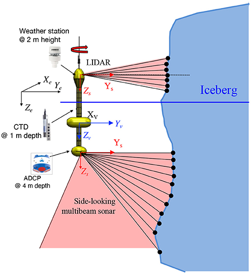
Figure 1. Sensor configurations on the USV SEADRAGON.

Here, three coordinate frames are defined. The earth-fixed coordinate frame (X_e − Y_e − Z_e) is selected in a North-East-Down (NED) convention with its x-axis pointing toward geographic North, y-axis pointing East, and z-axis pointing downward. The origin of this coordinate frame can be freely chosen but is fixed at the earth's surface with known latitude and longitude. The vehicle coordinate frame (X_v − Y_v − Z_v) is located at the center of gravity of the USV SEADRAGON with the x-axis pointing forward, y-axis pointing starboard, and z-axis pointing downward. For each sensor, we define a sensor coordinate frame (X_s − Y_s − Z_s) having the same orientation as the vehicle coordinate frame, but is offset by a translation vector ${}_s^v\text{T}$ from the origin of the vehicle coordinate frame.

More detailed information about the transformation between coordinate frames is presented in Supplementary Section 1. For a range vector, r_t, as reported by the sonar or the LIDAR at time t, we convert it into a point vector, ${}^v{\text{P}}_t$, in the vehicle coordinate frame using Equation (1) with σ_t being the angle between the range vector and X_s − Y_s plane and β_t being the angle between the range vector and Y_s − Z_s plane. The point vector, ${}^v{\text{P}}_t$, could be converted into the earth coordinate frame using Equation (2) where ϕ_t, θ_t, and ψ_t are the vehicle roll, pitch, and yaw, and ${}_v^e\text{T}$ is the displacement of the origin of the vehicle coordinate frame relative to the chosen origin of the earth-fixed coordinate frame.

$\begin{array}{ll}{}^v{\text{P}}_t={\text{R}}_z({\beta }_t){\text{R}}_x({\sigma }_t){\text{r}}_t{+}_s^v\text{T}& (1)\end{array}$

$\begin{array}{ll}{}^e{\text{P}}_t={\text{R}}_x({\varphi }_t){\text{R}}_y({\theta }_t){\text{R}}_z{({\psi }_t)}^v{\text{P}}_t{+}_v^e{\text{T}}_t& (2)\end{array}$

During operations, the USV SEADRAGON navigates using a Global Positioning System (GPS), located on the top deck. Its orientation is estimated using an Attitude Heading Reference System (AHRS) calibrated to the origin of the vehicle coordinate frame, at the center of gravity of the vehicle. The sonar and LIDAR both produce range measurements from the vehicle to the iceberg surface. The sonar is mounted on the lower hull with a vertical field-of-view on the starboard side of the vehicle. Its view angle covers from horizontal (0 deg) to 130 degrees downwards with a resolution of 1.8 degrees. The sonar data is processed in real-time with a sonar ping rate of 0.5 Hz at a profiling range of 150 m. The LIDAR is located on the top deck with the maximum profiling range of 100 m. It has a vertical field-of-view of 30 degrees with a 2-degree angular resolution, and it scans 360 degrees at 600 Revolution Per Minute (RPM) with a stepping angle of 0.4 degrees. In Supplementary Table 1, we present detailed information on the measurements and specifications of the sensors.

The range measurements obtained from the sonar and the LIDAR can be converted into the earth-fixed coordinate frame, creating a point cloud of the iceberg surface. However, because of the self-motion of the iceberg, the point cloud will be distorted in the earth-fixed coordinate frame representation. For shape representation, we introduce another coordinate frame the iceberg coordinate frame (X_b − Y_b − Z_b), as shown in Figure 2. Its origin is located at the centroid of the water-plane of the iceberg. The iceberg motion is constrained to three degrees of freedom, a northward speed, ${\stackrel{.}{x}}_b(t)$, an eastward speed, ${\stackrel{.}{y}}_b(t)$, and an angular velocity, ${\stackrel{.}{\psi }}_b(t)$ around the Z_b axis. The heaving, rolling and pitching motion can be neglected because our iceberg survey is conducted in less than 2 h, during a period of calm sea state. In addition, sea-state conditions under which the vehicle can conduct mapping mission will cause negligible iceberg rolling and pitching. To account for minor rolling, pitching or heaving, we implemented a gridding filter in section 3 to remove possible outliers.

FIGURE 2

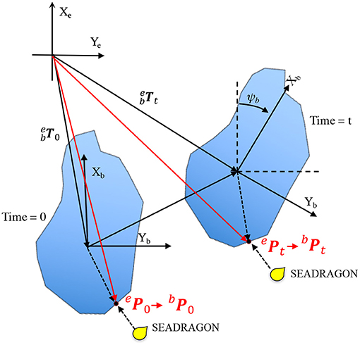
Figure 2. Iceberg coordinate frame moves and rotates in the Earth coordinate frame. An identical point is observed by the USV SEADRAGON at different time.

A top-view sketch of a moving iceberg is offered in Figure 2. At the beginning of the mission, t = 0, the iceberg coordinate frame is located at ${}_b^e{\text{T}}_0$ relative to the origin of the earth-fixed coordinate frame with the x-axis pointing north and y-axis pointing east. Equation (3) shows the conversion between a point in the iceberg coordinate frame and in the earth fixed coordinate frame. After the conversion, the resulting point cloud, ${}^b{\text{ℙ}}_{0:t}=\left\{{}^b{\text{P}}_0{,}^b{\text{P}}_1,{\dots }^b{\text{P}}_t\right\}$ presents the actual iceberg shape. Since instantaneous motion of the iceberg is not available, the integration of the iceberg motion in Equation (3) can be approximated with time averaged angular and linear velocities, ω_b(t), u_b(t), and v_b(t). The transformation between the coordinate frames is then rearranged through Equation (4), where the integration is replaced with the multiplication of time (t) and the averaged velocities, and the rotation matrix, ${\text{R}}_z^T$, is inverted. In the next section, we present an algorithm to estimate the averaged iceberg motion at different times such that all the points can be accurately converted into the iceberg-centered coordinate frame.

$\begin{array}{ll}{}^e{\text{P}}_t={\text{R}}_z^T\left({\displaystyle {\int }_0^t}{\stackrel{.}{\psi }}_b(t)\text{d}t\right){}^b{\text{P}}_t{+}_b^e{\text{T}}_0+\left[\begin{array}{c}{\int }_0^t{ẋ}_b(t)\text{d}t\\ {\int }_0^t{ẏ}_b(t)\text{d}t\\ 0\end{array}\right]& (3)\end{array}$

$\begin{array}{ll}{}^b{P}_t={(R_z^T)}^{-1}\left(t{\omega }_b(t)\right)\left({}^e{P}_t{-}_b^e{T}_0-t\left[\begin{array}{c}{u}_b(t)\\ v_b(t)\\ 0\end{array}\right]\right)& (4)\end{array}$

3. Iceberg Motion Estimation

In order to fully cover an iceberg, multiple circumnavigations are normally conducted during a survey. By detecting identical regions surveyed during different passes, iceberg motion information could be extracted for shape reconstruction. In our algorithm, we have a reference point cloud collected at the beginning of the mission, e.g., in the first 10 min. We refer the reference point cloud to as ${}^e{\text{ℙ}}_{0:t_0}$ where t₀ is the time-span that controls the point cloud size. Another point cloud is called the current point cloud referred to as ${}^e{\text{ℙ}}_{t-\Delta t:t}$ that is collected from time, t − Δt, to the current time, t. We denote that they are affiliated to the earth-fixed coordinate frame using the left superscript. The algorithm presumes that the two point clouds cover the same region on the iceberg; then, its objective is to search an iceberg motion solution that best aligns the two point clouds in the iceberg coordinate frame. We treat this process as an optimization problem inspired from the gradient descent method (Bryson and Ho, 1975). In addition, we designed a Kalman filter (KF) to fuse the iceberg motion estimates from the optimization into a linear iceberg motion model. Therefore, uncertainty in our motion estimation algorithm is also incorporated.

Figure 3 shows the flowchart for the overall motion estimation procedure. During initialization, we define several global parameters. The time coefficient, t₀, controls the size of the reference point cloud, Δt₀ controls the initial size of the current point cloud, α₁, α₂, and α₃ are the step sizes during the iterations. Also, we initialize the Kalman filter with the iceberg state, x₀, initial covariance, P₀, and innovation covariance, Q_k, as shown in Equation (5) and (6).

$\begin{array}{ll}{\text{x}}_0=\left[u_b,v_b,{\omega }_b,{\stackrel{.}{u}}_b,{\stackrel{.}{v}}_b,{\stackrel{.}{\omega }}_b\right]=0& (5)\end{array}$

$\begin{array}{ll}{\text{P}}_0={\text{I}}_{6\times 6}\text{and}{\text{Q}}_k=0.01{\text{ I}}_{6\times 6}& (6)\end{array}$

The next step is data preparation. Based on the time parameters, the program obtains two point clouds, ${}^e{\text{ℙ}}_{0:t_0}$ and ${}^e{\text{ℙ}}_{t-\Delta t:t}$. The algorithm will then perform down-sampling as follows:

1) The program will bin the two point clouds into 3-m depth bands starting from zero depth.

2) It will compare the total numbers of points within each depth bin, then, select the points inside the depth bin containing the highest numbers of data points.

3) The selected points will be further separated into 1-m 2D binned cells. For a cell that contains multiple data points, the associated timestamp of the latest observation will be kept. For LIDAR measurements, the program further filters the data set because outliers reflected from ships have been observed in the field experiment (see Figure 7 in section 4.2). Therefore, the cells that contain less than 25 observations are excluded.

FIGURE 3

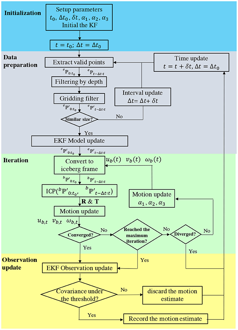
Figure 3. The flowchart of the motion estimation algorithm.

After the down-sampling, two new smaller point clouds, ${}^e{{\text{ℙ}}^{\prime }}_{0:t_0}$ and ${}^e{{\text{ℙ}}^{\prime }}_{t-\Delta t:t}$, are obtained. Before the iteration starts, the program will check if the size difference between them is less than 100. Otherwise, the program will update the time interval, Δt to increase the size of ${}^e{{\text{ℙ}}^{\prime }}_{t-\Delta t:t}$, and repeat the down-sampling procedures described above.

After proper point clouds have been identified, the algorithm will update the iceberg state and covariance in the KF as indicated in Equation (7) to (8) where the state matrix, F_k, is defined in Equation (9). The algorithm will then enter the iteration to search for the possible iceberg motion solution that matches the two input point clouds.

$\begin{array}{ll}{\widehat{\text{x}}}_{k|k-1}={\text{F}}_k{\widehat{\text{x}}}_{k-1|k-1}& (7)\end{array}$

$\begin{array}{ll}{\text{P}}_{k|k-1}={\text{F}}_k{\text{P}}_{k-1|k-1}{\text{F}}_k^T+{\text{Q}}_k& (8)\end{array}$

$\begin{array}{ll}{\text{F}}_k=\left[\begin{array}{cc}{\text{I}}_{3\times 3}& \delta t{\text{ I}}_{3\times 3}\\ 0_{3\times 3}& {\text{I}}_{3\times 3}\end{array}\right]& (9)\end{array}$

In each iteration, the program first converts the two point clouds into the iceberg coordinate frame based on the most-recent iceberg motion estimates. Then, it applies the Iterative Closest Point (ICP) algorithm (Bergstrom and Edlund, 2014) to compute the 2D rotation matrix, R, and the translation matrix, T, between two iceberg-related point cloud, ${}^b{{\text{ℙ}}^{\prime }}_{0:t_0}$ and ${}^b{{\text{ℙ}}^{\prime }}_{t-\Delta t:t}$. Based on the transformation information from the ICP, the program updates the iceberg motion, as shown in Equation (10), where α₁, α₂, and α₃ are the step size, and the subscript in R_2,1 indicates the row and column of the element. In the validation presented in section 4, α₁ and α₂ are defined to be 1/15,000. In contrast, α₃ is defined to be 1/150 because the rotation discrepancy has a smaller range from −1 to 1 compared to the range of T which is in the hundreds.

$\begin{array}{ll}\left[\begin{array}{c}{u}_b\\ v_b\\ {\omega }_b\end{array}\right]:=\left[\begin{array}{c}{u}_b\\ v_b\\ {\omega }_b\end{array}\right]-\left[\begin{array}{ccc}{\alpha }_1& 0& 0\\ 0& {\alpha }_2& 0\\ 0& 0& {\alpha }_3\end{array}\right]\left[\begin{array}{c}\text{T}\\ \\ {\text{R}}_{2,1}\end{array}\right]& (10)\end{array}$

At the end of each iteration, the program checks if the estimate is converged or diverged. A convergence is found if the most recent 50 estimates have a standard deviation of less than 10⁻⁵ m/s or 10⁻⁵deg/s. In contrast, if the estimation grows beyond a threshold, a divergence is found and the program will end the iteration with a conclusion of an invalid estimate. The program will then move to the next time step.

When testing the algorithm, we observed that the estimate overshoots before converging, especially when using a large step size. A large step size will result in a faster convergence but larger fluctuations and significant overshoot during iteration. Therefore, the iceberg motion threshold is set to ±3 m/s and ±3 deg/s to tolerate the large step size as needed for computational speed. A wider limitation would also allow our future investigation in the algorithm's performance on fast-moving and rotating objects besides icebergs. From the literature, iceberg drift was typically observed at 0.1 m/s in Robe (1980) and 0.3 m/s in Crawford et al. (2018), and rotational motion was observated at 0.003 deg/s (Crawford et al., 2018) and 0.005 deg/s (Kimball and Rock, 2011). It is clearly highly variable.

As illustrated in Figure 3, the program will perform a KF observation update only if the estimate has converged or the program has reached the defined maximum iteration (500 in our case). The observed iceberg velocity, u_b, v_b, ω_b, will be the mean values from the last 50 iterations, and the iceberg acceleration ${\stackrel{.}{u}}_b$, ${\stackrel{.}{v}}_b$, ${\stackrel{.}{\omega }}_b$ will be the iceberg velocity changes divided by the elapsed time since the last valid motion estimate. After that, the algorithm will update the iceberg states, ${\widehat{\text{x}}}_{k|k-1}$, and the covariance using Equations (11) and (13) with z_k being the iceberg motion observations from the iteration, K_k being the Kalman gain calculated in Equation (12), and H_k being the observation matrix. After the calculation, the iceberg motion states are updated from ${\widehat{\text{x}}}_{k|k-1}$ to x_k|k where the hat symbol denotes the difference between a model-predicted value and an observation-updated value. In Equation (12), the current covariance of the state estimation is P_k|k−1 that is later updated in Equation (13), and the measurement uncertainty is R_k, which is explained next.

$\begin{array}{ll}{\text{x}}_{k|k}={\widehat{\text{x}}}_{k|k-1}+{\text{K}}_k({\text{z}}_k-{\text{H}}_k{\widehat{\text{x}}}_{k|k-1})& (11)\end{array}$

$\begin{array}{ll}{\text{K}}_k={\text{P}}_{k|k-1}{\text{H}}_k^T{({\text{H}}_k{\text{P}}_{k|k-1}{\text{H}}_k^T+{\text{R}}_k)}^{-1}& (12)\end{array}$

$\begin{array}{ll}{\text{P}}_{k|k}=(\text{I}-{\text{K}}_k{\text{H}}_k){\text{P}}_{k|k-1}& (13)\end{array}$

Instead of defining a constant measurement uncertainty, the program determines R_k dynamically based on the output using ICP results. Previously during the iteration, we obtained a 2D rotation matrix, R and translation matrix, T. Now, we apply the ICP again but switch the reference and current point cloud around with current point cloud being the model and the reference point cloud being the data. By changing the initial condition, the program could detect local minima, which may provide a false matching solution in the ICP (Fitzgibbon, 2003). The second ICP application gives another transformation matrix, $\widehat{\text{R}}$ and $\widehat{\text{T}}$. The algorithm computes the observation uncertainty, R_k, using the two transformation matrices and a Sigmoid function, as shown in Equations (14) and (15) where the subscript in the transformation matrices indicates the row and column number of the element. The Sigmoid function could scale any real number into a specific bounded range to limit our measurement uncertainty in the KF. Here, we define the Sigmoid coefficients, a and b, which are equal to 0.1 and 100, respectively. The coefficients control the shape of the Sigmoid function curve. In our scenario, S(x) is converged to 1 when the input, x, is larger than 200. In the case that the ICP yields a large translation or rotation discrepancy between two point clouds, the corresponding measurement uncertainty will approach 1 which is 100 times larger than the innovation covariance shown in Equation (6). As a result, the iceberg motion found during the iteration will have less impact on the state update since the Kalman gain will approach 0 in Equation (12). After the observation update shown in Equations (11) and (13), the program will check the updated covariance. The program records the iceberg state estimate if all the diagonal elements in the state covariance, P_k|k, are less than 0.0049. This threshold value is determined based on the outcomes from running the algorithm offline. A larger value will result in more but nosier records of valid motion estimates, whereas a smaller value will result in less recorded motion estimates. For the simulation and the field data validation, we used the same value defined above. As indicated by the outermost feedback loop in Figure 3, the motion estimation algorithm runs at a constant interval, δt, which is set at 10 s in section 4.

$\begin{array}{ll}S(x)=\frac{1}{1+exp(-a(x-b))}& (14)\end{array}$

$\begin{array}{ll}\left[\begin{array}{c}{\sigma }^2(u_b)\\ {\sigma }^2(v_b)\\ {\sigma }^2({\omega }_b)\end{array}\right]=\left[\begin{array}{c}{\sigma }^2({\stackrel{.}{u}}_b)\\ {\sigma }^2({\stackrel{.}{v}}_b)\\ {\sigma }^2({\stackrel{.}{\omega }}_b)\end{array}\right]=\left[\begin{array}{c}S(|{\text{T}}_{1,1}\ast {\widehat{\text{T}}}_{1,1}|)\\ S(|{\text{T}}_{2,2}\ast {\widehat{\text{T}}}_{2,2}|)\\ S(|{sin}^{-1}({\text{R}}_{2,1})\ast {sin}^{-1}({\widehat{\text{R}}}_{2,1})|)\end{array}\right]& (15)\end{array}$

Of course, limitations exist in the proposed algorithm. First, the algorithm relies on the assumption that the iceberg surface is heterogeneous and irregular. Therefore, uniform objects, such as sphere and cubes, will cause ambiguous point cloud matching results, producing a false motion estimation. Moreover, different survey strategies will be required for larger systems, such as ice islands, because shape changes due to a “foot loose” mechanism (Wagner et al., 2014) and melting may happen between revolutions. As a result, the point matching algorithm proposed here may fail in finding the identical region from different revolutions. To overcome this limitation, repeated sectional iceberg scans may be conducted over a short time before there are significant shape changes. The proposed algorithm could then be used to estimate the ice-island drift by finding repeated features in different sectional scans. Finally, the sea state also affects the algorithm performance. The algorithm will work better at sea state equal or less than 4 (up to 2.5-m wave height). Such a limitation is determined based on the depth band (3 m) defined in the down-sampling and the assumption of negligible iceberg heave motion. With significant iceberg heave motion at higher sea state, the down-sampling may misrepresent a correct 2D cross-sectional profile at the selected depth. As a result, the iceberg motion estimated from matching two point clouds may contain increased errors. Moreover, excessive vehicle heaving motion caused by waves will influence the quality of the profiling sensors as well as the vehicle altitude estimate, which may downgrade the overall quality of the data product. To apply the algorithm to iceberg mapping data collected at higher sea states, one could extend the point cloud matching into 3D and include iceberg heave motion into the estimation. However, more computational resources are needed for 3D point cloud matching.

4. Algorithm Validation

4.1. Simulation

We have performed simulations in an iceberg mapping simulator (Zhou et al., 2014) with the ground truth iceberg shape from Barker et al. (1999) and a user-defined iceberg motion. Hence, we could compare the motion estimated from the proposed algorithm to the ground truth without considering any sensor-posed noise. In the simulation, an USV equipped with a side-looking multi-beam sonar is modeled. The vehicle is assumed moving at a constant speed of 1 m/s and follows the contour of the water-plane of the iceberg at a standoff distance of 50 m. The sonar is simulated with 45 rays equally separated from the horizontal direction to a downward-looking angle of 45 degrees. In the simulation, the iceberg is assumed to have a northward speed of 0.05 m/s, an eastward speed of 0.02 m/s and a clockwise rotational speed of 0.025 deg/s.

Figure 4A shows the top view of the resulting vehicle trajectory with the gray-scale color indicating the elapsed time. In the same figure, we also show the point cloud obtained from sonar range measurements, and the initial and final iceberg orientation and position. It can easily be seen that the point cloud representation in the North-East-Down coordinate frame is distorted due to the iceberg motion. Therefore, we applied the motion estimation algorithm in section 3 to derive the iceberg motion and restore the iceberg shape. The time related parameters in the algorithm are set as follows, t₀ = 600 Δt₀ = 120, and δt = 10, which are in seconds. Meanwhile, the dimensionless step sizes, α₁, α₂, and α₃ are set to 1/15,000, 1/15,000, and 1/150.

FIGURE 4

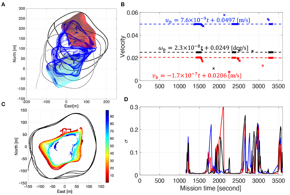
Figure 4. A summary of the results from the simulation data. Panel (A) shows the vehicle track (gray-scale track) and the iceberg surface measurements (blue dots) presented in the earth-fixed coordinate frame. The initial and ending iceberg pose is shown in cyan and red surface. Panel (B) shows the top view of the iceberg surface points and the vehicle track after iceberg motion correction. Panel (C) shows the recorded iceberg motion estimations (markers) extracted from the simulation data. The dashed lines and the equations show the least-squares fitting result with outlier detection enabled. Panel (D) shows the standard deviation of the iceberg velocity states over time.

Figure 4C shows the valid motion estimates during the mission. The dashed lines show the estimated time-varying iceberg drift equations which are derived by applying the least-square fitting with outlier detection enabled to the valid motion estimates (markers). The root-mean-square error normalized by the ground-truth value is 0.49, 1.7, and 0.25% for the northward, eastward and rotational velocities, respectively. As shown in Figure 4C, the algorithm has identified three loop-closure occurrences, around 1,500, 2,500, and 3,300 s. This agrees with the simulation where the vehicle circumnavigated the moving iceberg four times.

With the estimated iceberg velocity shown in Figure 4C, we have converted all iceberg surface points into the iceberg coordinate frame using Equation (4). The motion-corrected iceberg point cloud is presented in Figure 4B with a color scheme showing the points at different depth and the black track presents the vehicle track relative to the iceberg. We compared this point cloud with our ground truth iceberg profile in the CloudCompare software (CloudCompare, 2019) using the default method, the nearest neighbor distance. Figure 5A shows the histogram of the distance errors, where the 99.7% line is located at 8.3 m and the mean value is around 3 m. Meanwhile, Figure 5B depicts the spatial distribution of distance errors.

FIGURE 5

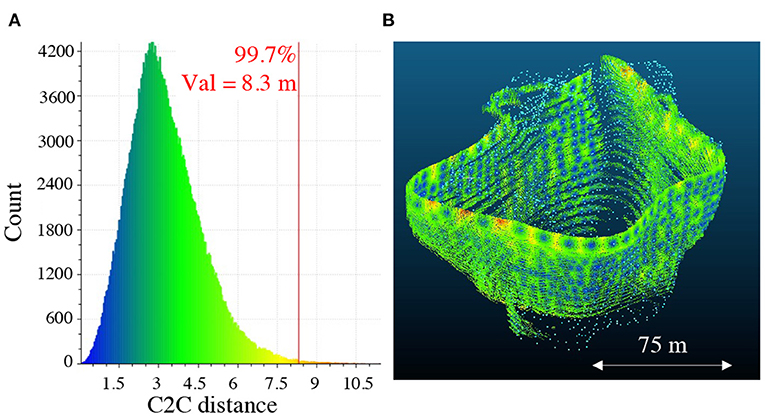
Figure 5. Distance error between the reconstructed point cloud and the ground truth point cloud. Panel (A) Shows the histogram of the separation distance between the restored iceberg point cloud and the actual iceberg shape. Panel (B) shows the color-coded distance errors in the reconstructed point cloud.

4.2. Field Experiment

In June 2017, the USV SEADRAGON was deployed to map a floating iceberg near Portugal Cove (47.637 N 52.883 W), Newfoundland, Canada. Figure 6 shows the four images taken from different directions around the target iceberg. The height of the iceberg gradually decreases from the South to the North end with a concave feature on the Northern side. The above-water portion is about 120 m long, 100 m wide, and 20 m high. The water depth in the area exceeds 60 m allowing for iceberg drift. In the Supplementary Figure 3, we presented the raw sonar point cloud in the earth coordinate frame where the seafloor topography could be observed.

FIGURE 6

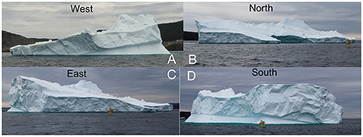
Figure 6. Above water iceberg shape shown in four images taken from different directions (A–D).

As shown previously in Figure 1, the USV carries a LIDAR and a side-looking multi-beam sonar for profiling the above and below water portion of the iceberg. For environmental assessment, a weather station, a downward-looking Acoustic Doppler Current Profiler (ADCP), a conductivity-temperature-depth (CTD) sensor was operational during the trial. In Supplementary Section 2, we summarize the sensor configuration for the iceberg mapping mission.

Figure 7 shows the vehicle track (black lines) and the iceberg surface measurements obtained from the sonar and the LIDAR. All these measurements are presented in the North-Earth-Down coordinate frame with the origin located at 47.626^oN 52.875^oW. The iceberg drifted toward the Northeast during the survey. Overall, the vehicle circled around the iceberg 4 times for about 1.5 h. A wall-following algorithm was implemented to maintain the desired standoff distance of 50 m with minimum human control. Such a standoff distance was determined such that LIDAR (maximum 100 m range) and sonar (maximum 300 m range) could both collect sufficient measurements for cross-validation. The wall-following algorithm uses the local iceberg profile from the LIDAR scans. The LIDAR acquired data is collapsed onto the horizontal plane to present the local 2D iceberg contour. From the collapsed data, the desired vehicle track is generated by shifting the contour toward the vehicle. The line-of-sight guidance law (Norgren and Skjetne, 2015) was used to compute the low-level heading commands based on the desired track. Manual control was required several times during the mission because the algorithm misinterpreted other targets, e.g., ships, detected by the LIDAR. This problem can be solved by integrating a high-level system to manage vehicle operations in the presence of marine craft or other obstacles, e.g., by limiting the LIDAR scanning angle.

FIGURE 7

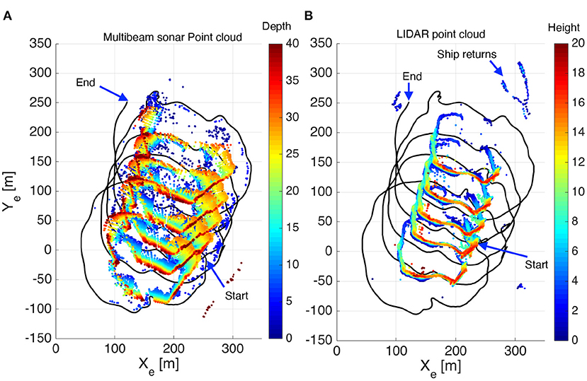
Figure 7. The topview of the point cloud collected from the multi-beam sonar (A) and the LIDAR (B). The vehicle trajectory is shown in black.

We applied the motion estimation algorithm to the two separated data sets collected by the LIDAR and the sonar. The initial time is set to be the sonar on time, UTC 15:23:19. The time parameter, t₀, for the reference point cloud is 1,100 s while other parameters remain unchanged from the simulation.

The left panel of Figure 8 shows the motion estimated from the two data sets, while the linear equation parameters are summarized in the right panel of Figure 8. Comparing the results obtained from the LIDAR and sonar dataset, we found that (1) both estimations show a decrease in the iceberg drift, and (2) more valid estimates and smaller uncertainty are obtained from the LIDAR point cloud because LIDAR data has less noise and higher data density than the sonar measurements.

FIGURE 8

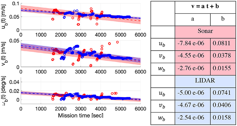
Figure 8. The left panel shows the motion estimated from the sonar (red) and LIDAR (blue) datasets. The markers show the valid estimates, the dashed lines show the curve fitting results with shaded area indicating the 95% confidence zone. Right panel summarizes the parameters of the dashed lines.

Next, we convert the two point clouds shown in Figure 7 into the iceberg coordinate frame using the velocity functions presented in Figure 8. The overall motion-corrected point cloud and vehicle track are shown in Figure 9. We separated the data into 1-m cubic bins to reduce computer memory. We removed outliers manually in MeshLab (MeshLab, 2018). The left panel in Figure 9 shows the isometric view of the processed point cloud, while the right panel shows the top view of the point cloud with the iceberg-referenced vehicle trajectories. The observed freeboard portion (topside) has an averaged height of 6.9 m with a maximum value of 21 m. As mentioned in Rackow et al. (2017), the draft (D) of an iceberg can be estimated with the equation D = Hρ_i/ρ_w, where H is overall height of the iceberg, ρ_i is the density of the iceberg, and ρ_w is the density of the water. Using the mentioned equation and the freeboard measurements, the draft is estimated to be 57 m with ρ_i being 850kg/m³ (Silva et al., 2006) and ρ_w being 1, 024.7kg/m³ from the CTD measurements on the USV. In the USV observation, the below water portion has an averaged depth of 19.8 m and a maximum observed draft of 48 m. There are two main reasons that can explain the difference between the observed draft (48 m) and the estimated draft (57 m). On the observation side, the actual keel of the iceberg may be deeper than 48 m given the seafloor depth lies between 60 and 85 m shown in Supplementary Figure 3. This occurs mainly because the USV is limited to move at the water surface. As a result, the distance between the USV and the deeper portion of the iceberg may exceed the sonar range, and the increased angle of incident at the sonar footprint on the iceberg at the deeper depth will cause low acoustic returns (sonar dropouts). On the other hand, Rackow et al. (2017) assumed that the iceberg is in cubic shape rather than the ram shape observed by the USV. Therefore, the relation between the drag (D), above-water height (F), water density, and the iceberg density will be slightly different for our data set.

FIGURE 9

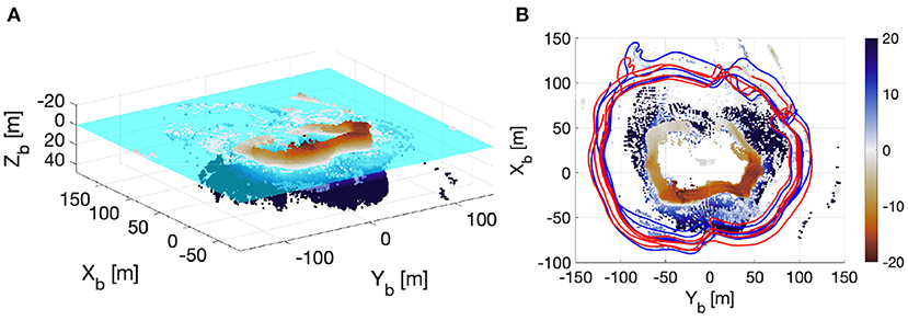
Figure 9. Processed iceberg point cloud shown in the isometric view (A) and top view (B). The red and blue tracks in (B) shows the vehicle tracks corrected using the iceberg velocity estimates obtained from the sonar and LIDAR dataset, respectively.

Next, we assumed that our reconstructed iceberg represents the actual shape.

We computed the overall volume of the below-water (5.12 × 10⁵m³) and the above-water portion (8.31 × 10⁴m³) with the assumption that the iceberg is in 1-m stacked layers. Based on the volume and the Archimedes' principle, the iceberg density is estimated to be 881kg/m³. If the deeper portion of this iceberg is not mapped by the USV, the potentially unmapped portion will create a positive buoyant to the overall iceberg. In order maintain the same freeboard volume that is fully observed, the iceberg has to be denser. Therefore, 881kg/m³ will be the lower bound of the density of the mapped iceberg which is denser than Antarctic icebergs (850kg/m³ mentioned in Silva et al., 2006) and somewhat closer to other icebergs observed in the Labrador Sea (910kg/m³ mentioned in Barker et al., 2004).

Figure 10 presents a local comparison between two subsets of iceberg points. The blue and the red point cloud are collected from 2,000 to 3,000 s and 3,000 to 4,000 s, respectively. The measurements from 10 m depth to the height of 5 m were excluded since they are noisy due to the signal reflections from the ship and the water surface. The point clouds were also gridded into 1-cubic meter bins. We computed the distance between two above-water subsets and two below-water ones in the CloudCompare (CloudCompare, 2019) with the nearest neighbor distance. In Figure 10, we show histograms of the distance errors for the above-water and below-water portion. Overall, the maximum mismatching between the two subsets is about 9 m. We observed that the misalignment in the LIDAR point clouds is slightly smaller than that from the sonar point clouds where the error is up to 10 m.

FIGURE 10

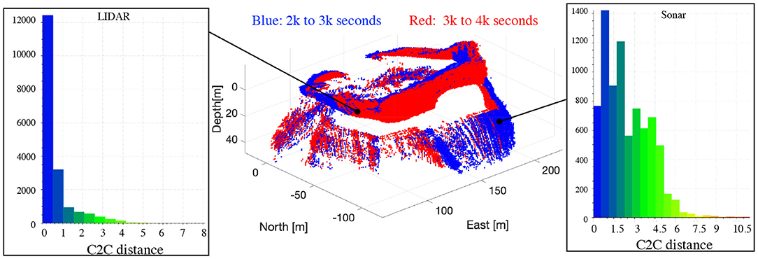
Figure 10. Comparing the point clouds collected between 2,000–3,000 and 3,000–4,000 s after the correction for the iceberg motion. The data points are binned into 1-m cubic cells.

Finally, we applied the surface reconstruction method (Zhou et al., 2019) to the processed point cloud. Figure 11 shows multiple views of the final iceberg rendering. The resulting shape is comparable to the photos shown in Figure 6. In Supplementary Figure 4, the common features in the iceberg render and the pictures in Figure 6 are highlighted.

FIGURE 11

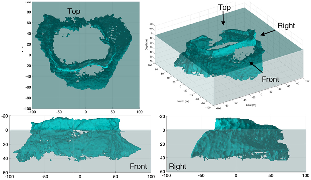
Figure 11. Multiple views of the reconstructed iceberg shape.

5. Field Environmental Observations

During the iceberg mapping experiment, the USV SEADRAGON was also equipped with other scientific instruments, including a RDI ADCP (600k Hz), a Seabird pumped CTD and an Airmar Weather Station. The locations of these sensors are depicted in Figure 1. In this section, we present the collected scientific measurements and derive iceberg melting estimates.

The ADCP data was first corrected for the vehicle motion (velocity and orientation) using the USV's GPS and the AHRS measurements. The ocean current velocity is then corrected for the iceberg's translational speed (estimated in section 4.2). After these corrections, we obtained the ocean current velocity relative to the iceberg. Next, we performed a moving average at 3 min interval in each depth bin (2 m) to eliminate the wave disturbances. After that, we binned the ocean current measurements based on the depth (2 m) and its azimuth angle (1 deg) relative to the origin of the iceberg. Finally, we applied 2D Gaussian filtering (Shapiro and Stockman, 2001) to smooth the binned data with the final result shown in Figure 12 where the overall ocean current around the iceberg is presented. The left, middle, and right plots present the Northward, Eastward and Downward components of the processed ocean current. From these color plots, we could observe that the water is mainly following toward Northwest with small sections of Southward and Eastward flow, which may be caused by the turbulence induced by the iceberg. Interestingly, the water in the upstream is found moving downward in contrast to the upwelled water found in the downstream on the Northeast side. This finding agrees with the iceberg mechanism discussed in Stern et al. (2015) and Moon et al. (2018). The other discovery is the upwelled water in the deeper portion (around 50 m) in the upstream. This may occur due to the basal iceberg melting that produces a buoyant water mass.

FIGURE 12

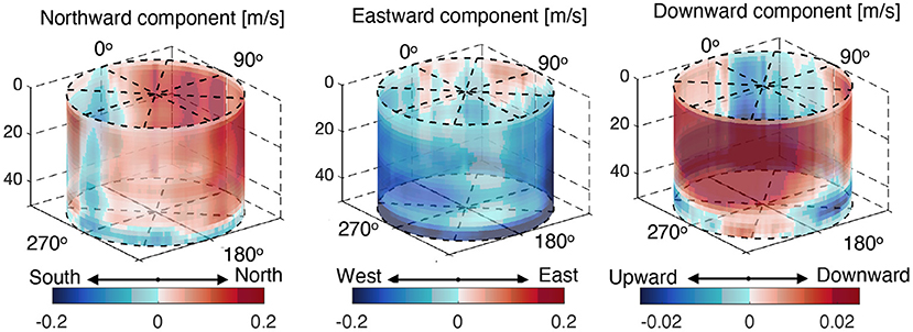
Figure 12. The averaged velocity of the water flowing around the iceberg. The row indicates the different revolutions while the column indicates the velocity components in Northward, Eastward, and downward directions.

In Figure 13, we show the processed CTD, current and wind measurements in 1-cubic meter bins. In each bin, the value is the mean of all the data points in the bin. In Figures 13A,B, the surface water temperature and salinity are measured by the CTD (submerged at 1 m) on the USV. A water plume that is 1 degree colder and slightly fresher was identified in the downstream of the iceberg. We attribute this anomaly to the iceberg melting and heat flux. Figure 13C shows the depth-averaged current derived from Figure 12. The length of the arrows presents the magnitude of the planar component, and the color indicates the depth-averaged vertical components. In Figure 13D, we show the airflow around the iceberg. The weather station was sampling at 2 Hz, and we applied the moving average to the value at 3 min intervals (same as the ADCP processing) before gridding. Overall, the wind is blowing toward Northeast with a difference of about 2 m/s in speed between the windward and the leeward side. We found the iceberg drifting direction (about 28 degrees from North to the East), estimated in section 4.2, is more coincident with the wind blowing direction rather than the current flowing direction (toward Northwest), which is also discussed by Wagner et al. (2017) using an analytical iceberg drift model.

FIGURE 13

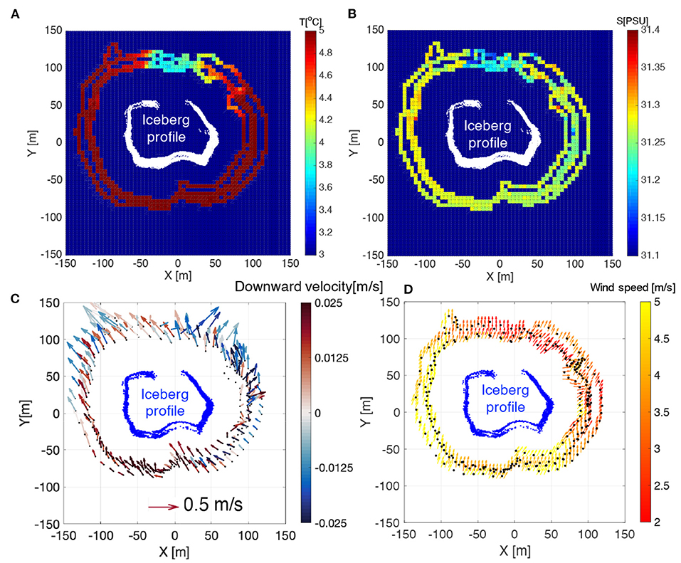
Figure 13. The surface water temperature (A), salinity (B), current field (C), and wind pattern (D) around the USV SEADRAGON. The data are averaged value in 1-cubic meter bins.

Combining all these environmental measurements, we further quantified relevant melting characteristics. Instead of taking the mean value of water properties, we estimated the melting parameters in different iceberg sections as different water properties, current, wind, temperature, and salinity, resulting in uneven iceberg melting affecting the iceberg stability and resulting in iceberg rolling. Stern et al. (2015) presented an approach to compute the melting metrics for an iceberg. Here, we estimate the melting caused by the surface wave erosion and the sensible heat flux in both above and below water. For the underwater portion, we only included the results from the mapped portion up to the maximum observed draft (48 m).

The ocean current estimates in Figure 12, water temperature and salinity in Figures 13A,B, and the wind speed in Figure 13 (D) are used in our melting estimation. These measurements are separated into different sections (10 degrees each) based on the azimuthal angle relative to the origin of the iceberg coordinate frame that is located at the geometry center of the iceberg cross-section at zero depth. In each section, we computed the mean water temperature, T(θ); salinity, S(θ); water pressure, P(θ); water density, ρ_w(θ); the depth-averaged current, V_b(θ); and wind speed, V_a(θ). Using the binned point cloud shown in Figure 9, we computed the sectional iceberg surface area above and below the water, A_a(θ) and A_b(θ), and the effective area for the surface wave erosion, A_s(θ). For simplicity, we approximated the iceberg into 1-m stacked layers. In each layer, the cross-section remains the same. Therefore, the total surface area is the sum of the sectional contour lengths multiplied by the layer height.

For each section, we computed the deterioration rate due to the surface wave erosion and the melt rates due to sensible heat flux. The deterioration rate (Equation 16) caused by the surface wave erosion, ṁ_s was about 1 m/day per degree above the freezing temperature (Savage, 2001; Scambos et al., 2008). The freezing temperature, T_f, is related to the salinity and water pressure. From our CTD measurements, T_f is estimated to be about −1.7 degrees. Here, we only consider the effective area of the wave erosion is from 5 m above the water (average height) to 15 m (assumed thermocline boundary). The effective area will be later used when computing the total melt volume in Equation (19).

$\begin{array}{ll}{ṁ}_s(\theta )=T(\theta )-T_f(S(\theta ),P(\theta ))& (16)\end{array}$

$\begin{array}{ll}{ṁ}_a(\theta )=\frac{1}{L{\rho }_i}{\rho }_a{c}_{pa}A{V}_a(\theta )(T(\theta )-T_{fa})& (17)\end{array}$

$\begin{array}{ll}{ṁ}_b(\theta )=\frac{1}{L{\rho }_i}{\rho }_w(\theta )c_{pw}S{t}_{\ast }\sqrt{C_d}{V}_b(\theta )(T(\theta )-T_f(S(\theta ),P(\theta ))& (18)\end{array}$

$\begin{array}{ll}\stackrel{.}{V}={\displaystyle \sum _{\theta =0^o}^{360^o}}\frac{{\rho }_i}{{\rho }_w(\theta )}({ṁ}_s(\theta )A_s(\theta )+{ṁ}_a(\theta )A_a(\theta )+{ṁ}_b(\theta )A_b(\theta ))& (19)\end{array}$

Above the water, the melt rate due to the sensible heat transfer is given by Equation (17), where the numerator is the sensible heat flux with ρ_a being the air density, c_pa being the specific heat of air, A being the dimensionless transfer coefficient for air, T_fa being the freezing temperature in air. In the denominator, L is the latent heat of fusion of ice, ρ_i is the iceberg density. For the below-water portion, the melt rate due to the sensible heat is given by Equation (18) where the numerator is the sensible heat flux with c_pw being the specific heat of the water, St_* being the Stanton number (McPhee, 1992), C_d being the drag coefficient (Stern et al., 2015), T_f being the freezing point of the water. The total melt volume is then computed using Equation (19) from the melt rates and the related iceberg surface area. Using the coefficients presented in Stern et al. (2015), we computed the mentioned iceberg melting parameters given by Equation (16) to (19). All the constants and related parameters used in the computation are summarized in Supplementary Table 4.

In Figure 14, we present the melt rates and total melt volume in 10-degree sections around the iceberg. We observed that the melt rate due to the sensible heat flux above the water, ṁ_a(θ), is much higher on the southern side due to the high wind speed observed in Figure 13D. In contrast, the below water melt rate due to the sensible heat flux is higher in the downstream on the Northwest side due to the higher flow speed shown in Figure 13C. The deterioration caused by the surface wave is more evenly distributed due to the small temperature difference of about 1.2 degrees. Overall, the below-water melt rate due to the sensible heat flux is about ten times higher than that for the above-water part. The total melt volume around the iceberg is also presented in the top-right plot in Figure 14. The melt volume is observed higher on the Northwest, Southwest and Southeast side where larger iceberg surface area are found either underwater (top-middle plot in Figure 14) or above the water (top-left plot in Figure 14). The inconsistent melting, both around the iceberg and between above and below water, reveals an uneven iceberg shape changes that can cause iceberg instability and lead to possible iceberg rolling events. By summing the sectional melt volume, the total melt volume is estimated to be 1.088 × 10⁵m³/day. For comparison, the total iceberg volume of the mapped portion is about 5.87 × 10⁵m³.

FIGURE 14

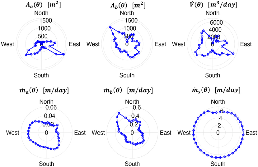
Figure 14. Melt related parameters at different azimuth angle (θ) around the iceberg. A_a(θ) and A_b(θ) are the above-water and below-water surface area, ${\stackrel{.}{V}}_{\theta }$ is the total melt volume, and ṁ_a(θ), ṁ_b(θ), and ṁ_s(θ) are the melt rates caused by above-water sensible heat, below-water sensible heat, and the wave erosion.

6. Conclusion and Future Work

In this paper, we have presented an approach to profiling floating icebergs using an unmanned surface vehicle (USV), the USV SEADRAGON. Our work has an emphasis on estimating iceberg motion and characterization of the iceberg shape.

First, we presented an algorithm to estimate iceberg motion which is needed to correctly reconstruct the shape of surveyed icebergs. During the implementation, we added a down-sampling method to reduce the computational cost and time. The algorithm was running on a typical PC (3.1 GHz Dual-Core Intel i7 and 16GB 1867MHz DDR3) in data playback mode. We believe that the algorithm is applicable for in-situ computation on an embedded computer that could be integrated onto marine robotic platforms for real-time processing. Instantaneous results will greatly help in-situ decision making for iceberg management and adapting strategies of sampling the surrounding water near an iceberg, e.g., conducting follow-up measurements on the freshwater plume in the downstream.

The algorithm was first evaluated with a simulated data set based on a real iceberg shape without sensor noise. We simulated the iceberg translation and rotational motion during the simulation. The algorithm has successfully detected the loop-closure from consecutive revolutions with a maximum normalized RMS error under 2% between the estimated motion and the simulated values. Such an estimation error caused a misalignment up to 8 m between the estimated iceberg shape and the ground truth shape (presented in Figure 5). Subsequently, the algorithm has been applied to the field data collected by the USV SEADRAGON in June 2017. The presented algorithm successfully extracted the iceberg drift, both translation and rotation, which is further used for iceberg shape reconstruction and iceberg melt studies.

Meteorological and oceanographic data collected by the USV SEADRAGON was analyzed. This data provides a detailed picture of the environment around the iceberg. We have discovered several important features, such as freshwater pond and upwelling water in the downstream. We also reveal inconsistent melting parameters between above and below portion around the iceberg, which can lead to iceberg instability that may cause a roll-over event. Overall, the total melt volume is estimated to be 1.088 × 10⁵m³/day with a volume of about 5.87 × 10⁵m³ from the mapped portion, from 20 m above-water to 50 m under the water. At the estimated melt rate and measured volume, the lifespan of the iceberg will be less than 6 days.

While these results for iceberg reconstruction and melting estimates are promising, more measurements and data are still needed to understand the iceberg melting mechanism, e.g., the vertical extent of the freshwater plume and its influence to iceberg deterioration. We propose the following future research directions to advance the iceberg mapping and relevant scientific studies. The results presented in this paper showed that a side-looking multi-beam sonar attached to a surface vehicle is not sufficient to obtain the overall submerged shape because of the sonar dropouts at greater depth due to the increased grazing angle. We, therefore, propose to combine the surface vehicle with a sonar-equipped autonomous underwater vehicle (AUV) in order to profile the deeper regions of the iceberg. Explorations with field experiments have already been conducted by Zhou et al. (2019), McEwen et al. (2018), and Forrest et al. (2012). Complementary to direct measurements, artificial intelligence algorithms may be developed to predict the “missing” portion based on the survey data. The algorithm would reconstruct the unsurveyed portion based on established iceberg stability conditions and empirical equations, such as the stability theories discussed by EL-Tahan and EL-Tahan (1982). For iceberg deterioration studies, we suggest performing more CTD casts in the downstream in order to quantify the water mass at increased spatial and temporal resolution. In order to do that, a new type of platform may be necessary to accommodate the horizontal moving mode and the vertical profiling mode, such as the vehicle designed by Bachmayer et al. (2018).

Data Availability Statement

The raw data supporting the conclusions of this article will be made available by the authors, without undue reservation.

Author Contributions

RB and BY were the leading PIs on the iceberg mapping project. The algorithm development and the data analysis was conducted by MZ under the supervision of RB and BY. MZ wrote the initial manuscript while RB and BY offered the edits, comments on the revisions, and manages a private Github repository for all the code. All authors contributed to the article and approved the submitted version.

Funding

This research was supported by the Ocean Industries Student Research Award (OISRA) awarded by the Newfoundland Research & Development Corporation (RDC), the Natural Sciences and Engineering Research Council Canada (NSERC) through the NSERC Canadian Field Robotics Network (NCFRN), Memorial University of Newfoundland, the Atlantic Canada Opportunities Agency, the Government of Newfoundland and Labrador.

Conflict of Interest

The authors declare that the research was conducted in the absence of any commercial or financial relationships that could be construed as a potential conflict of interest.

Acknowledgments

The authors thank the funding agencies for the support, the Marine Institute for providing the ship for the field trial, and all the engineers in from the Autonomous Ocean Systems Laboratory for supporting the SEADRAGON deployment. The author would like to thank for the reviewers' insightful comments that greatly improved this paper.

Supplementary Material

The Supplementary Material for this article can be found online at: https://www.frontiersin.org/articles/10.3389/fmars.2021.549566/full#supplementary-material

References

Bachmayer, R., de Young, B., Lewis, R., Wang, H., MacNeil, L., Sobalski, V., et al. (2018). “The idea, design and current state of development of an unmanned submersible surface vehicle: USSC seaduck,” in 2018 IEEE/OES Autonomous Underwater Vehicle Workshop (AUV) (Porto). doi: 10.1109/AUV.2018.8729732

CrossRef Full Text | Google Scholar

Barker, A., Sayed, M., and Carrieres, T. (2004). “Determination of iceberg draft, mass and cross-sectional areas,” in The Fourteenth International Offshore and Polar Engineering Conference (Toulon), 899–904.

Google Scholar

Barker, A., Skabova, I., and Timco, G. (1999). Iceberg Visualization Database. PERD/CHC Report, National Research Council Canada.

Google Scholar

Bergstrom, P., and Edlund, O. (2014). Robust registration of point sets using iteratively reweighted least squares. Comput. Optimizat. Appl. 58, 543–561. doi: 10.1007/s10589-014-9643-2

CrossRef Full Text | Google Scholar

Bruneau, A. A., and Dempster, R. T. (1972). “Engineering and economic implications of icebergs,” in North Atlantic, Conf. Pop. Oceanology Int. (Brighton), 176–180.

Bryson, A., and Ho, Y. (1975). Applied Optimal Control: Optimization, Estimation, and Control. Hemisphere Publishing Corporation.

Google Scholar

Canatec (2015). UAV Ice Beacon. Available online at: http://www.canatec.ca/wp-content/uploads/2015/07/UAV-Ice-Beacon.pdf

CloudCompare (2019). Cloud Compare (Version 2.9.1) [GPL Software]. Available online at: www.cloudcompare.org

Crawford, A., Mueller, D., and Joyal, G. (2018). Surveying drifting icebergs and ice islands: deterioration detection and mass estimation with aerial photogrammetry and laser scanning. Remote Sens. 10:575. doi: 10.3390/rs10040575

CrossRef Full Text | Google Scholar

Crocker, G., Wright, B., and Bruneau, S. (1998). An Assessment of Current Iceberg Management Capabilities. Contract Report for National Research Council Canada.

Eik, K. (2008). Review of experiences within ice and iceberg management. J. Navigat. 61, 557–572. doi: 10.1017/S.0373463308004839

CrossRef Full Text | Google Scholar

EL-Tahan, M., and EL-Tahan, H. (1982). “Estimation of iceberg draft,” in MTS/IEEE OCEANS'82 (Washington, DC). doi: 10.1109/OCEANS.1982.1151865

CrossRef Full Text | Google Scholar

Farmer, L., and Robe, R. (1975). “Volumetric measurements of icebergs,” in The 3rd International Conference on Port and Ocean Engineering under Arctic Conditions (Fairbanks, AK), 188–199.

Fitzgibbon, A. (2003). Robust registration of 2D and 3D point sets. Image Vis. Comput. 21, 1145–1153. doi: 10.1016/j.imavis.2003.09.004

CrossRef Full Text | Google Scholar

Forrest, A., Schmidt, V., Laval, B., and Crawford, A. (2012). “Digital terrain mapping of petermann ice island fragments in the Canadian high Arctic,” in 21st IAHR International Symposium on Ice (Dalian).

Google Scholar

Gladstone, R. M., Bigg, G. R., and Nicholls, K. W. (2001). Iceberg trajectory modeling and meltwater injection in the southern ocean. J. Geophys. Res. Oceans 106, 19903–19915. doi: 10.1029/2000JC000347

CrossRef Full Text | Google Scholar

Hammond, M., Clark, A., Mahajan, A., Sharma, S., and Rock, S. (2015). “Automated point cloud correspondence detection for underwater mapping using AUVs,” in MTS/IEEE Oceans 2015 (Washington, DC). doi: 10.23919/OCEANS.2015.7404431

CrossRef Full Text | Google Scholar

Hammond, M., and Rock, S. M. (2014a). “Enabling AUV mapping of free-drifting icebergs without external navigation aids,” in IEEE/MTS Oceans 2014 (St. John's, NL). doi: 10.1109/OCEANS.2014.7003145

CrossRef Full Text | Google Scholar

Hammond, M., and Rock, S. M. (2014b). “A slam-based approach for underwater mapping using AUVs with poor inertial information,” in 2014 IEEE/OES Autonomous Underwater Vehicles (AUV) (Oxford, MS). doi: 10.1109/AUV.2014.7054419

CrossRef Full Text | Google Scholar

Hodgson, G., Lever, J., Woodworth-Lynas, C., and Lewis, C. (1998). Dynamics of Iceberg Grounding and Scouring Volume 1 - The Field Experiment. Environmental Studies Research Funds.

International Ice Patrol (2014). Report of the International Ice Patrol In the North Atlantic 2014 Season.

Jansen, D., Schodlok, M., and Rack, W. (2007). Basal melting of A-38B: a physical model constrained by satellite observations. Remote Sens. Environ. 111, 195–203. doi: 10.1016/j.rse.2007.03.022

CrossRef Full Text | Google Scholar

Kimball, P., and Rock, S. (2008). “Sonar-based iceberg-relative AUV navigation,” in 2008 IEEE/OES Autonomous Underwater Vehicles, AUV 2008 (Woods Hole, MA). doi: 10.1109/AUV.2008.5290534

CrossRef Full Text | Google Scholar

Kimball, P., and Rock, S. (2011). Sonar-based iceberg-relative navigation for autonomous underwater vehicles. Deep Sea Res. II 58, 1301–1310. doi: 10.1016/j.dsr2.2010.11.005

CrossRef Full Text | Google Scholar

Kimball, P., and Rock, S. (2015). Mapping of translating, rotating icebergs with an autonomous underwater vehicle. IEEE J. Ocean. Eng. 40, 196–208. doi: 10.1109/JOE.2014.2300396

CrossRef Full Text | Google Scholar

Larssen, G. (2015). Ice Detection and Tracking Based on Satellite and Radar Images. Department of Marine Technology, Faculty of Engineering Science and Technology, Norwegian University of Science and Technology.

Google Scholar

Marko, J., Birch, J., and Wilson, M. (1986). A study of long-term satellite-tracked iceberg drifts in Baffin Bay. Arctic 35, 234–240. doi: 10.14430/arctic2322

CrossRef Full Text | Google Scholar

McEwen, R. S., Rock, S. P., and Hobson, B. (2018). “Iceberg wall following and obstacle avoidance by an AUV,” in 2018 IEEE/OES Autonomous Underwater Vehicle Workshop (AUV) (Porto: IEEE). doi: 10.1109/AUV.2018.8729724

CrossRef Full Text | Google Scholar

McPhee, M. G. (1992). Turbulent heat flux in the upper ocean under sea ice. J. Geophys. Res. 97, 5365–5379. doi: 10.1029/92JC00239

CrossRef Full Text

MeshLab (2018). MeshLab. Available online at: http://www.meshlab.net

Google Scholar

Moon, T., Sutherland, D., Felikson, D. C., Kehrl, L., and Straneo, F. (2018). Subsurface iceberg melt key to greenland fjord freshwater budget. Nat. Geosci. 11, 49–54. doi: 10.1038/s41561-017-0018-z

CrossRef Full Text | Google Scholar

Norgren, P., and Skjetne, R. (2014). Using autonomous underwater vehicle as sensor platforms for ice-monitoring. Model. Identif. Control 35, 263–277. doi: 10.4173/mic.2014.4.4

CrossRef Full Text | Google Scholar

Norgren, P., and Skjetne, R. (2015). Line-of-sight iceberg edge-following using an auv equipped with multibeam sonar. IFAC Pap. Online 48, 81–88. doi: 10.1016/j.ifacol.2015.10.262

CrossRef Full Text | Google Scholar

Norgren, P., and Skjetne, R. (2018). A multibeam-based slam algorithm for iceberg mapping using auvs. IEEE Access 6, 26318–26337. doi: 10.1109/ACCESS.2018.2830819

CrossRef Full Text | Google Scholar

Rackow, T., Wesche, C., Timmermann, R., Hellmer, H. H., Juricke, S., and Jung, T. (2017). A simulation of small to giant Antarctic iceberg evolution: differential impact on climatology estimates: melt and drift of small to giant icebergs. J. Geophys. Res. Oceans 122, 3170–3190. doi: 10.1002/2016JC012513

CrossRef Full Text | Google Scholar

Rignot, E., and Kanagaratnam, P. (2006). Changes in the velocity strucutre of the greenland ice sheet. Science 311, 986–990. doi: 10.1126/science.1121381

PubMed Abstract | CrossRef Full Text | Google Scholar

Rignot, E., Velicongna, I., van den Broeke, M., Monaghan, A., and Lenaerts, J. (2011). Acceleration of the contribution of the greenland and antarctic ice sheets to sea level rise. Geophys. Res. Lett. 38, 1–5. doi: 10.1029/2011GL046583

CrossRef Full Text | Google Scholar

Robe, R. Q. (1980). “Iceberg drift and deterioration,” in Dynamics of Snow and Ice Masses. Academic Press. doi: 10.1016/B978-0-12-179450-7.50009-7

CrossRef Full Text | Google Scholar

Savage, S. B. (2001). Aspects of iceberg deterioration and drift. Geomorphol. Fluid Mech. 582, 279–318. doi: 10.1007/3-540-45670-8_12

CrossRef Full Text | Google Scholar

Scambos, T., Ross, R., Bauer, R., Yermolin, Y., Skvarca, P., Long, D., et al. (2008). Calving and ice-shelf break-up processes investigated by proxy:antarctic tabular iceberg evolution during northward drift. J. Glaciol. 54, 579–591. doi: 10.3189/002214308786570836

CrossRef Full Text | Google Scholar

Shapiro, L. G., and Stockman, G. C. (2001). Computer Vision. Prentice Hall.

Google Scholar

Silva, T. A., Bigg, G. R., and Nicholls, K. W. (2006). Contribution of giant icebergs to the southern ocean freshwater flux. J. Geophys. Res. Oceans 111:C03004. doi: 10.1029/2004JC002843

CrossRef Full Text | Google Scholar

Smith, N., Li, Z., Bachmayer, R., and Luchino, F. (2014). “Development of a semi-submersible unmanned surface craft,” in IEEE/MTS Oceans'14 (St. John's, NL). doi: 10.1109/OCEANS.2014.7003265

CrossRef Full Text | Google Scholar

Stern, A., Johnson, E., Holland, D. M., Wagner, T. J., Wadhams, P., Bates, R., et al. (2015). Wind-driven upwelling around grounded tabular icebergs. J. Geophys. Res. Oceans 120, 5820–5835. doi: 10.1002/2015JC010805

CrossRef Full Text | Google Scholar

Wagner, T. J., Dell, R. W., and Eisenman, I. (2017). An analytical model of iceberg drift. J. Phys. Oceanogr. 47, 1605–1616. doi: 10.1175/JPO-D-16-0262.1

CrossRef Full Text | Google Scholar

Wagner, T. J. W., Wadhams, P., Bates, R., Elosegui, P., Stern, A., Vella, D., et al. (2014). the “footloose” mechanism: iceberg decay from hydrostatic stresses. Geophys. Res. Lett. 41, 5522–5529. doi: 10.1002/2014GL060832

CrossRef Full Text | Google Scholar

Zhou, M., Bachmayer, R., and deYoung, B. (2014). “Initial performance analysis on underside iceberg profiling with autonomous underwater vehicle,” in IEEE/MTS Oceans'14 (St. John's, NL).

Google Scholar

Zhou, M., Bachmayer, R., and deYoung, B. (2016a). “Adaptive heading controller on an underwater glider for underwater iceberg profiling,” in Arctic Technology Conference 2016 (St. John's, NL). doi: 10.4043/27471-MS

CrossRef Full Text | Google Scholar

Zhou, M., Bachmayer, R., and deYoung, B. (2016b). “Towards autonomous underwater iceberg profiling using a mechanical scanning sonar on a underwater slocum glider,” in IEEE/OES Autonomous Underwater Vehicle (AUV) (Tokyo). doi: 10.1109/AUV.2016.7778656

CrossRef Full Text | Google Scholar

Zhou, M., Bachmayer, R., and deYoung, B. (2019). Mapping the underside of an iceberg with a modified underwater glider. J. Field Robot. 36, 1102–1117. doi: 10.1002/rob.21873

CrossRef Full Text | Google Scholar