 Thomas G. Bell1,2*
 Jack G. Porter2
 Wei-Lei Wang2Michael J. Lawler2
 Emmanuel Boss3
 Michael J. Behrenfeld4
 Eric S. Saltzman2
- 1Plymouth Marine Laboratory, Plymouth, United Kingdom
- 2Department of Earth System Science, University of California, Irvine, Irvine, CA, United States
- 3School of Marine Sciences, University of Maine, Orono, ME, United States
- 4Department of Botany and Plant Pathology, Oregon State University, Corvallis, OR, United States
This work presents an overview of a unique set of surface ocean dimethylsulfide (DMS) measurements from four shipboard field campaigns conducted during the North Atlantic Aerosol and Marine Ecosystem Study (NAAMES) project. Variations in surface seawater DMS are discussed in relation to biological and physical observations. Results are considered at a range of timescales (seasons to days) and spatial scales (regional to sub-mesoscale). Elevated DMS concentrations are generally associated with greater biological productivity, although chlorophyll a (Chl) only explains a small fraction of the DMS variability (15%). Physical factors that determine the location of oceanic temperature fronts and depth of vertical mixing have an important influence on seawater DMS concentrations during all seasons. The interplay of biomass and physics influences DMS concentrations at regional/seasonal scales and at smaller spatial and shorter temporal scales. Seawater DMS measurements are compared with the global seawater DMS climatology and predictions made using a recently published algorithm and by a neural network model. The climatology is successful at capturing the seasonal progression in average seawater DMS, but does not reproduce the shorter spatial/temporal scale variability. The input terms common to the algorithm and neural network approaches are biological (Chl) and physical (mixed layer depth, photosynthetically active radiation, seawater temperature). Both models predict the seasonal North Atlantic average seawater DMS trends better than the climatology. However, DMS concentrations tend to be under-predicted and the episodic occurrence of higher DMS concentrations is poorly predicted. The choice of climatological seawater DMS product makes a substantial impact on the estimated DMS flux into the North Atlantic atmosphere. These results suggest that additional input terms are needed to improve the predictive capability of current state-of-the-art approaches to estimating seawater DMS.
Introduction
The surface oceans are universally supersaturated with DMS relative to the overlying atmosphere, inducing a flux of approximately 28 Tg S yr –1 into the atmosphere (Lana et al., 2011). The sea-to-air flux of DMS is the largest biological source of sulfur to the marine atmosphere and the principle precursor of non-sea-salt sulfate in marine aerosols. These non-sea-salt sulfate aerosols are a significant contributor to cloud condensation nuclei (CCN) number and influence cloud radiative properties (Charlson et al., 1987). DMS in surface waters is the product of numerous biotic and abiotic processes, and surface ocean levels reflect production and destruction in the water column as well as loss to the atmosphere (Galí and Simó, 2015). Regional and seasonal variations of DMS in seawater reflect both physical (mixing, light, temperature) and biological (community structure, physiology) processes.
The North Atlantic Ocean experiences a widespread and highly productive seasonal phytoplankton bloom. Previous observations show large seasonal changes in North Atlantic surface ocean DMS concentrations (Lana et al., 2011) and DMS-derived sulfate is a significant component of the North Atlantic mass of submicron marine aerosol (Sanchez et al., 2018; Quinn et al., 2019). Models also indicate a strong climate sensitivity to regional DMS emissions (Carslaw et al., 2013; Woodhouse et al., 2013; Mahajan et al., 2015). Correlations between satellite remote sensing of cloud radiative properties and ocean color in the North Atlantic region have been used to argue in support of a biological impact on cloud properties (Falkowski et al., 1992). However, documenting the linkages between surface ocean biological activity and overlying aerosol/cloud properties with direct observations is challenging in the highly dynamic North Atlantic environment. The mechanistic links between atmospheric DMS and new particle formation are uncertain (see Quinn and Bates, 2011), particularly given the recent identification of novel DMS oxidation products (Veres et al., 2020).
One of the objectives of the North Atlantic Aerosols and Marine Ecosystems Study (NAAMES) was to explore ecosystem/aerosol/cloud linkages in the North Atlantic Ocean (NAAMES; see Behrenfeld et al., 2019). As part of that study, surface ocean DMS concentrations were measured continuously during four shipboard field campaigns in the NW Atlantic over a 4 year period (2015–2018). The cruises targeted the key stages of the annual phytoplankton bloom (the winter transition, accumulation, climax, and declining phases). Reduced sulfur cycle measurements have been made in the same region in May, July, and October 2003 (Scarratt et al., 2007; Lizotte et al., 2008, 2012; Merzouk et al., 2008). The authors demonstrated a link between plankton community composition and the major biological precursor to DMS (dimethylsulfoniopropionate, DMSP). Environmental parameters such as photosynthetically active radiation (PAR), sea surface temperature (SST), and mixed layer depth (MLD) were also important in determining seawater DMS.
The aim of this paper is to present an overview of the seawater DMS observations during NAAMES and some of the environmental factors that influence DMS variability. In particular, we focus on ancillary observations that can be made from space. NAAMES DMS measurements are also compared to estimates of DMS variability using a semi-empirical algorithm (Galí et al., 2018) and a neural network model (Wang et al., 2020). A future study will focus on how the NAAMES data can be used to improve predictions of seawater DMS.
Materials and Methods
Field Data Collection
Four field campaigns were conducted in the NW Atlantic on the R/V Atlantis: NAAMES1 (5th November–2nd December 2015), NAAMES2 (11th May–5th June 2016), NAAMES3 (30th August–24th September 2017) and NAAMES4 (20th March–13th April 2018). The cruises began and ended in Woods Hole (Massachusetts, United States), with the exception of NAAMES4, which started in San Juan, Puerto Rico and ended in Woods Hole (Figure 1). A complete description of the participants and methodologies employed on NAAMES is given by Behrenfeld et al. (2019). Each NAAMES expedition spent about 2 weeks occupying 5–7 stations in the region from 40 to 50°N along 40°W. The latitudinal gradients along this transect enabled a space-for-time approach that provided samples at different developmental stages of the phytoplankton annual cycle (Behrenfeld et al., 2019).
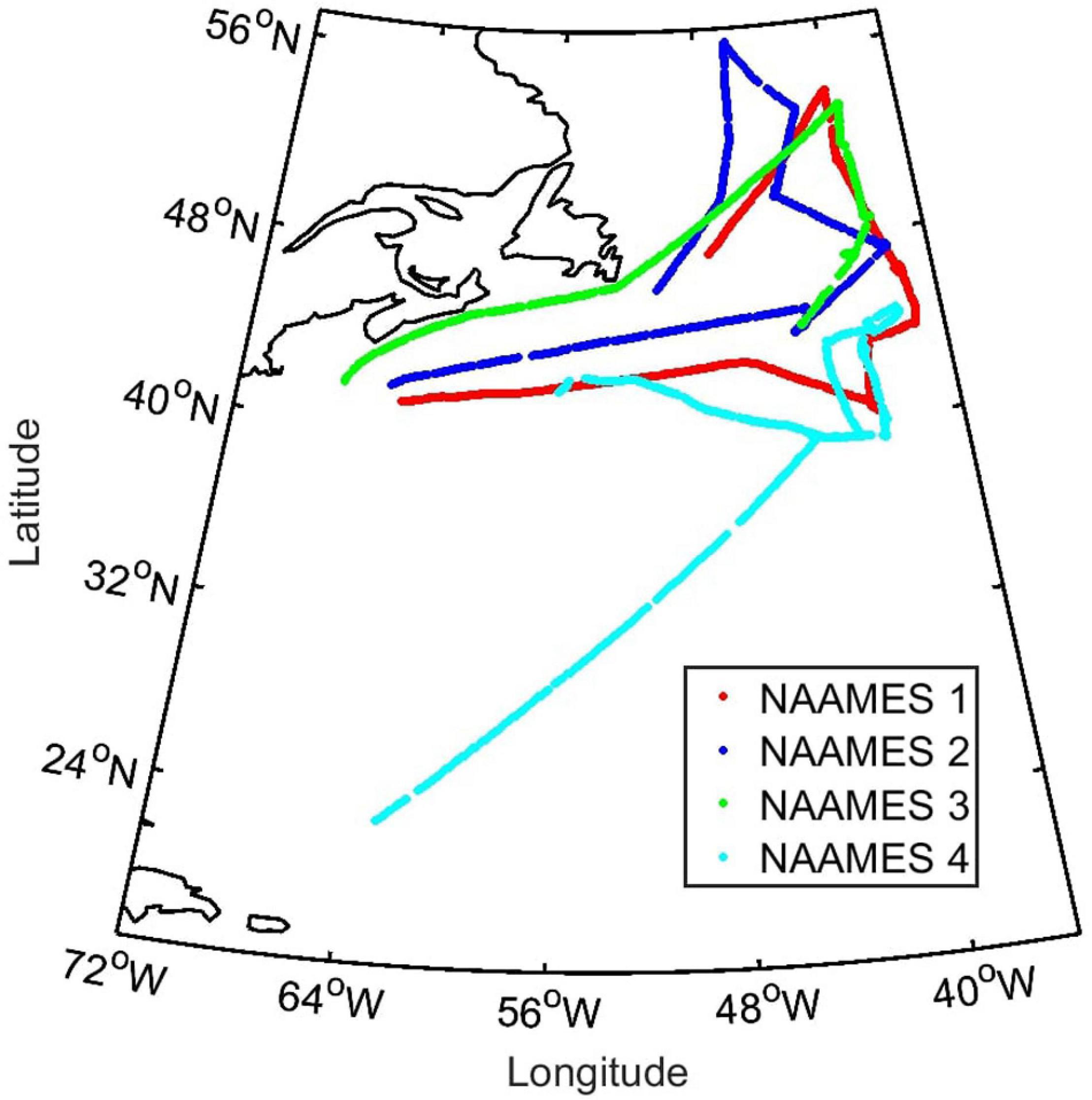
Figure 1. Data collection locations on all NAAMES cruises. NAAMES1 (5th November–2nd December 2015; red), NAAMES2 (11th May–5th June 2016; blue), NAAMES3 (30th August–24th September 2017; green), and NAAMES4 (20th March–13th April 2018; cyan).
CTD profiles and water samples were collected at each station for analysis of plankton stocks, rates, physiology and community composition, and seawater physico-chemical and optical properties. Analyses were also carried out on seawater sampled from the continuously pumped, non-toxic underway supply of the Atlantis. A peristaltic pump for the non-toxic seawater supply was specifically installed during the NAAMES cruises to minimize disruption to the biological community. Samples were collected to characterize the plankton, with Chl estimated from hyperspectral particulate attenuation and absorption (Wetlabs ACS). Chl concentration was derived from the continuous optical data after tuning to the NAAMES region with pigment (HPLC) data (see Fox et al., 2020, for more details). SST measurements were made at 1 Hz with a hull sensor (Seabird SBE 48).
Seawater DMS measurements were made continuously on the underway seawater supply on all four cruises, except during periods of instrument downtime (Figure 1). Seawater DMS data were thus collected before, during, and after the CTD stations.
Seawater DMS Measurements
DMS was measured using a miniCIMS: an atmospheric pressure chemical ionization mass spectrometer coupled to a counterflow membrane equilibrator (for details, see Saltzman et al., 2009). The equilibrator consists of a porous PTFE membrane tube housed within a larger non-porous PFA Teflon tube. High purity air flows inside the porous membrane and seawater counterflows around it. DMS exchanges across the permeable membrane, causing the exiting air stream to approach equilibrium with the entering seawater. The air flow to the equilibrator is mass flow controlled at 0.4 L min–1. The seawater flow rate is approximately 4 L min–1, continuously logged with an ultrasonic flow meter (Cynergy3 UF08B). Upon exiting the equilibrator, the air flow is passed through a Nafion membrane drier, and diluted with 1.1 L min–1 high purity air. The air stream is directed into the heated (300°C), atmospheric pressure ion source of the mass spectrometer. Ionization is carried out by passage of the air over a radioactive 63Ni foil. The ionized gas stream is drawn into the mass spectrometer through a pinhole, and declustered at approximately 1 Torr. A modified residual gas analyzer (Stanford Research Systems RGA-200, containing a quadrupole, and ion multiplier) is used to mass filter and detect DMS as the (CH3SCH3).H+ ion.
A primary, isotope-labeled, aqueous standard (triple deuterated DMS: 43.2 mM d3-DMS) was made prior to each cruise in a gas tight bottle using ethanol as the solvent. DMS is highly soluble in ethanol and thus very little DMS is lost into any headspace that develops. Fresh working standards were prepared daily by diluting 150 μl of primary standard in deionized water. A gas-tight Hamilton syringe was used to pierce the butyl rubber septa of the primary standard bottle and transfer d3-DMS into a working standard syringe containing 50 mL deionized water. Working standard (130 μM d3-DMS) was continuously delivered at 30 μL min–1 by a syringe pump (New-Era NE300) into flowing seawater before it reached the equilibrator.
Variations in the d3-DMS signal demonstrate that the standard was stable. The signal before/after daily syringe changes indicate working standard stability over the course of a day. The signal from newly made working standard was indistinguishable from the 24 h-aged standard signal. Primary standards were kept away from the light and there is no indication that the primary standard degraded over the course of a cruise. The non-isotopic DMS and d3-DMS signals gradually increased during the cruise compared to the signals at the beginning. Overall positive trends in DMS signals were observed during every NAAMES cruise and we attribute this to a gradual improvement in instrument sensitivity. Contaminants with a high proton affinity such as ammonia efficiently scavenge protons from charged water clusters and suppress the DMS signal. High purity air flowing continuously through the measurement tubing and instrument gradually removes contaminants attached to the tubing and instrument walls and the DMS signal increases commensurately.
Seawater DMS concentration (DMSSW) is calculated as follows:
where Sig63 and Sig66 represent the average blank-corrected ion currents (pA) of protonated DMS (CH3SCH3H+; m/z = 63) and d3-DMS (CD3SCH3H+; m/z = 66), respectively, CStd is the concentration of d3-DMS liquid standard (nM); FStd is the syringe pump flow rate (L min–1); and FSW is the seawater flow rate (L min–1).
DMS and d3-DMS were monitored in single ion mode at a frequency of at least 0.5 Hz. NAAMES1 measurements are reported as 5 min averages. The miniCIMS was also used to monitor seawater acetone concentrations during subsequent cruises (NAAMES2–4, results to be discussed in a later publication). The measurements during NAAMES2–4 are 10 min averages, with the instrument alternating between a dried (DMS measurements) and undried (acetone measurements) sample gas stream every 20 min.
A previous intercomparison compared DMS concentrations from the UCI miniCIMS system with results from another seawater measurement technique (Walker et al., 2016). A purge and trap system coupled to a sulfur chemiluminescence detector analyzed discrete water samples from the underway system of a research vessel in the Southern Ocean. The miniCIMS measured DMS in the underway water at the same time as the discrete samples were collected. The data from the two techniques compared well, with a mean residual difference of 1.2 nM (<15% bias). Previous seawater DMS intercomparison exercises have shown agreement within ± 25% (Bell et al., 2012; Swan et al., 2014).
Satellite Data for Seawater DMS Prediction
The following MODIS-Aqua level 3 remote sensing products (10.5067/AQUA/MODIS/L3M) were utilized in this study: SST, Chl, and daily PAR. Monthly composite data were used for NAAMES1 (November 2015), NAAMES2 (May 2016), and NAAMES3 (September 2017). NAAMES4 began in March and ended in April, so a composite product was generated from three 8 day data retrievals (collected between 22nd March 2018 and 14th April 2018). The composite data were required to minimise the patchiness due to clouds in individual 8 day data retrievals. Regional North Atlantic data were extracted from the remote sensing products for statistical analysis. Two areas, a rectangle (36–65°W, 39–43°N) and a square (36–51°W, 43–57°N), were selected and combined to encompass the majority of the NAAMES cruise tracks and to cover the wider North Atlantic region. MODIS SST, Chl, and PAR data were extracted along the NAAMES cruise tracks using the SeaDAS software package (Baith et al., 2001). Gridded sea surface height anomalies (SSHA) are derived by the NASA JPL MEaSUREs project using reference data from TOPEX/Poseidon, Jason-1, Jason-2, and Jason-3 (Zlotnicki et al., 2016).
In situ and Regional DMS Predictions Using Empirical and Neural Network Models
Galí et al. (2018) parameterized seawater DMS using PAR and total DMSP (DMSPt):
where PAR is the daily mean along-ship track MODIS product and DMSPt was predicted using in situ SST, Chl, euphotic zone depth (Zeu), and MLD data (Galí et al., 2015). The choice of DMSPt algorithm is dependent on euphotic zone depth (Zeu) and MLD, which were used to determine whether the water column was stratified (Zeu/MLD > 1) or mixed (Zeu/MLD < 1):
Euphotic zone depth (Zeu) was estimated as a function of Chl, following Morel et al. (2007):
where ζ = log10(Chl). Galí et al. (2015) also estimated Zeu from Chl using Eqn. 5. We chose this in preference to the satellite-derived estimate of Zeu used by Galí et al. (2018). An estimate of Zeu using in situ measurements should be more accurate over smaller spatial and temporal scales than a satellite-derived estimate. Note that Galí et al. (2018) will be referred to as G18 for the rest of this paper.
CTD profiles were collected when the ship was on station, such that there are only relatively few in situ MLD estimates. In addition, MLDs were extracted from a climatology generated using profiles from the Argo float program and a density algorithm for MLD detection (Holte and Talley, 2009; Holte et al., 2017). The MLD input term in Galí et al. (2018) was the Monthly Isopycnal / Mixed-layer Ocean Climatology (MIMOC), which uses multiple data streams including the Argo float data (Schmidtko et al., 2013). All MLD estimates (for in situ CTD, Argo climatology, and MIMOC data) were made using the same density algorithm.
For NAAMES1–3 there was reasonable agreement between the MLDs derived from CTD and Argo profiles (Supplementary Figures S1, S2). The agreement was not as good for NAAMES4. CTD data were only available from the first half of NAAMES4, during which Argo MLDs are much deeper than the CTD MLDs. G18-predicted DMS was calculated using CTD MLDs as well as using Argo MLDs. The G18 predictions calculated using in situ and climatological MLD products are compared and discussed in the Results.
An artificial neural network model was used to estimate DMS concentrations. We use an adapted version of the (Wang et al., 2020) neural network model, with sampling time and location parameters, SST, salinity, Chl, PAR, and MLD all used as potential predictors. The major notable change from Wang et al. (2020) is that we chose not to use nutrients as input variables. Excluding climatological nutrient fields from the analysis ensured that the G18 and neural network predictions used similar input variables and were driven by variables that can be retrieved using satellite and autonomous assets. Model output was not substantially changed by excluding nutrients.
The neural network model was developed using 93,571 data points: 86,785 from the global DMS database1 and 6,786 from NAAMES project. Not all data was used to develop the model, with a certain proportion initially left out for internal testing (∼10%) and external validation (∼13%). The internal testing and validation datasets were not selected at random because using near-neighbor values produces an overfitted model (as discussed in Wang et al., 2020). In situ SST and salinity data collected concurrently with DMS measurements were used for the model wherever possible. Average monthly climatological products were used when in situ data were not available. In addition to the in situ data, the model was developed with climatological Chl and PAR data from satellite and MLD from the MIMOC climatology (Schmidtko et al., 2013). For further detail on the artificial neural network model, the reader is referred to Wang et al. (2020) and to the model code (available at2).
G18 and the neural network model were used to produce regional maps of predicted DMS. The regional map predictions used climatological input fields of SST, Chl and PAR (MODIS), salinity (Garcia et al., 2013) and MLD (MIMOC). The MODIS satellite data products are those detailed in the previous section so the regional DMS outputs match the observation periods of the NAAMES cruises. North Atlantic surface ocean DMS was also extracted from the global seawater DMS climatology (Lana et al., 2011; hereafter referred to as L11).
DMS Flux Calculation
The DMS flux (FluxDMS) calculation uses the thin film model first proposed by Liss and Slater (1974):
where K is the gas transfer velocity and ΔDMS is the air-sea concentration difference. Atmospheric DMS levels were orders of magnitude lower than those in water during NAAMES (Quinn et al., 2019). We thus omit atmospheric DMS from our calculations and assume DMSSW ≈ΔDMS. The gas transfer velocity (K) is estimated as a function of wind speed adjusted to a 10 m measurement height and a neutral stability atmosphere (U10n) following Goddijn-Murphy et al. (2012):
where U10n is calculated from in situ wind speed observations and the COAREG model (Fairall et al., 2011). The in situ Schmidt number for DMS (ScDMS, the diffusivity of DMS through seawater) is used to adjust K at a reference Schmidt number (Sc = 660) to a K specific to DMS at the in situ SST. ScDMS is dependent upon seawater temperature (SST, °C) and was calculated from Saltzman et al. (1993) as follows:
Results
North Atlantic Regional Features
Composite MODIS SST (Figure 2) and Chl (Figure 3) provide a spatial context for data collected along each NAAMES cruise track. The satellite products and shipboard data clearly show the strong North-South SST gradient and the transport of warm, sub-tropical water toward the European continent by the Gulf Stream during all four cruises. Gulf Stream meandering generates warm and cold water eddies and temperature fronts along its boundary. The mesoscale and sub-mesoscale variability driven by meanders, eddies and fronts affects phytoplankton abundance and community composition (McGillicuddy, 2016). Oceanic (sub)mesoscale variability has a strong influence on the physical, chemical and biological properties of waters along the NAAMES 40°W North-South transects (see Della Penna and Gaube, 2019).
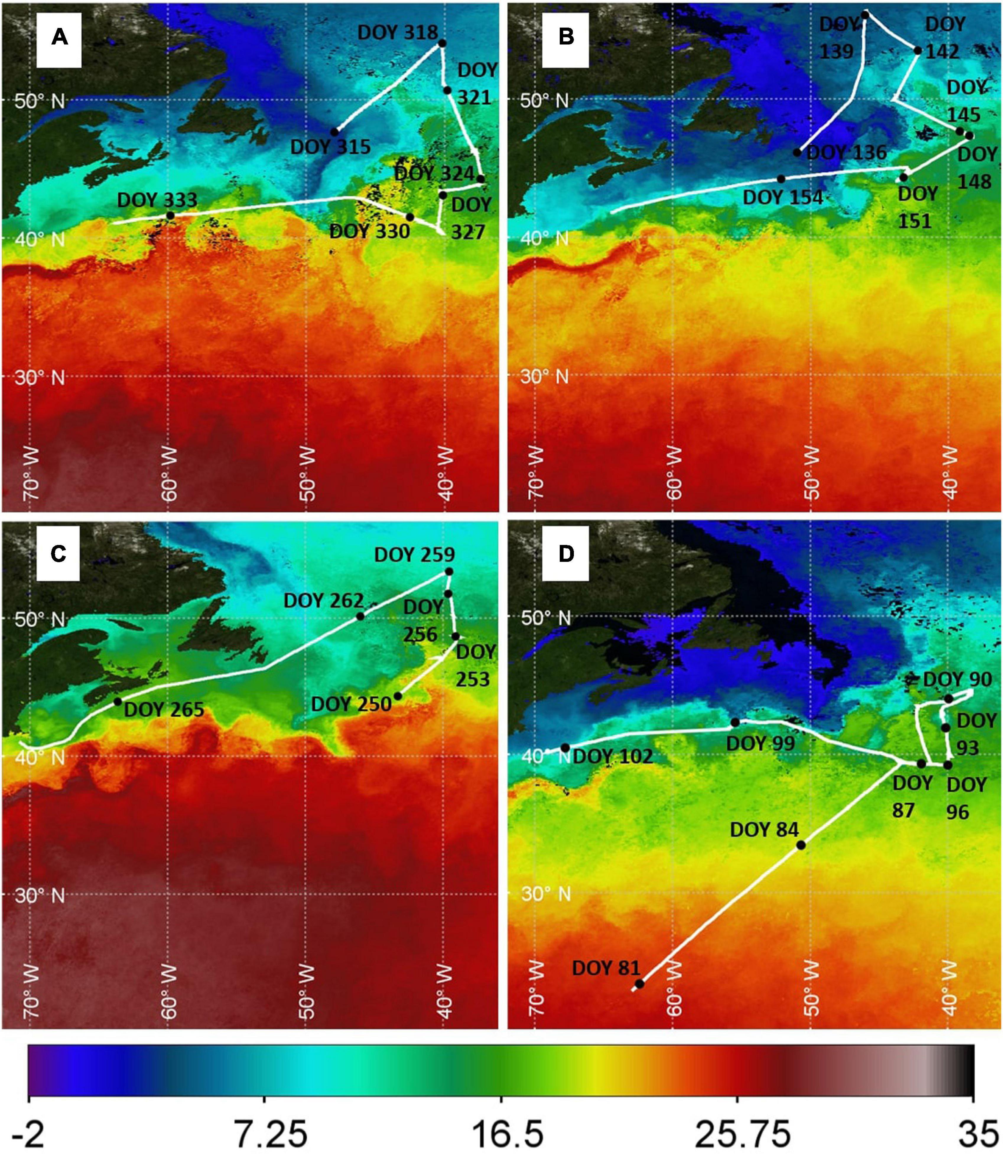
Figure 2. Composite MODIS sea surface temperature (SST, °C) data products for each cruise. (A) NAAMES1: November, 2015; (B) NAAMES2: May 2016; (C) NAAMES3: September 2017; and (D) NAAMES4: March/April 2018. Locations where DMS data were collected are shown (solid white line) with black dots indicating the ship position (labels indicate the Day of Year, DOY).
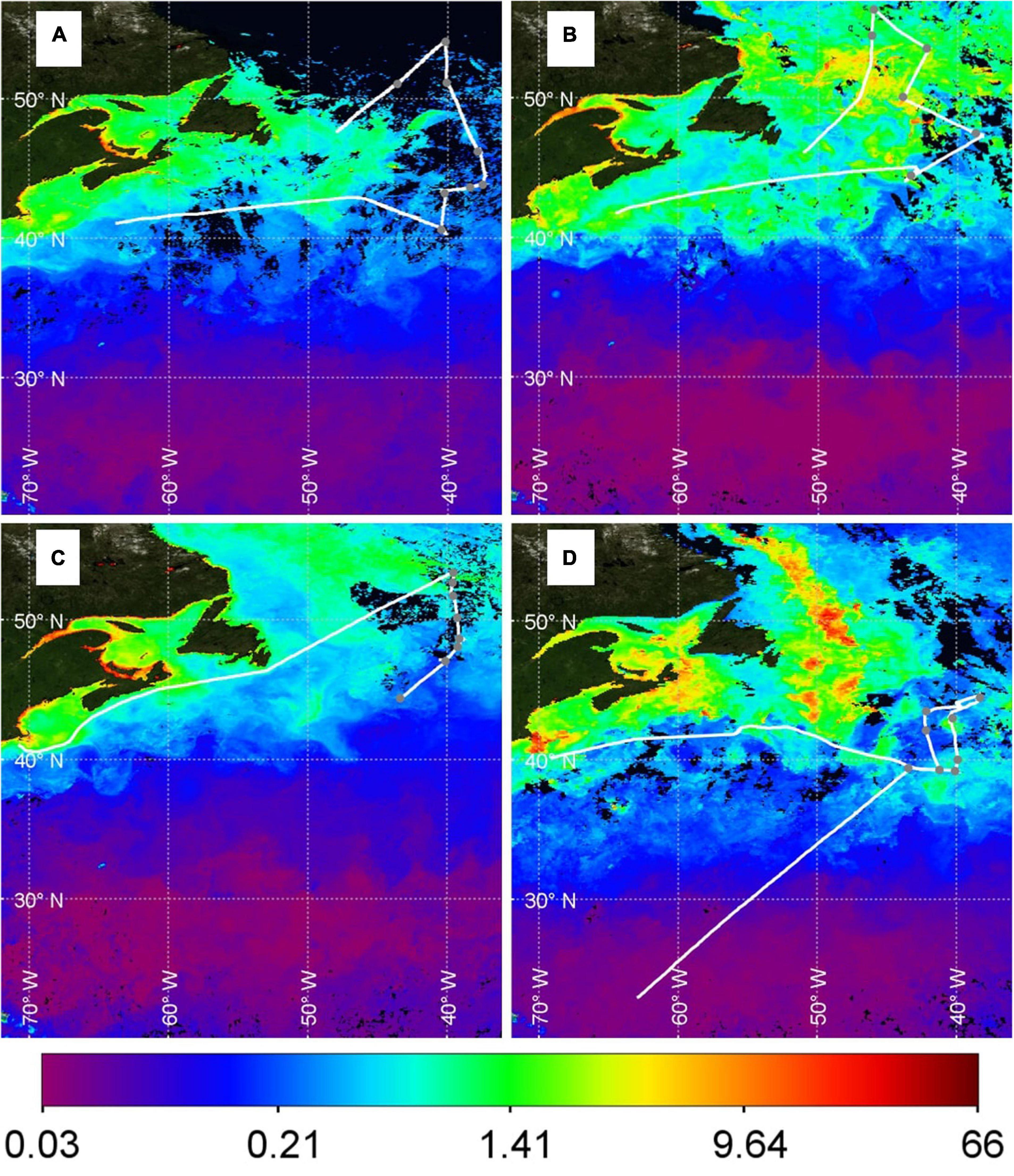
Figure 3. Composite MODIS chlorophyll (Chl, mg/m3) data products for each cruise. (A) NAAMES1: November, 2015; (B) NAAMES2: May 2016; (C) NAAMES3: September 2017; and (D) NAAMES4: March 2018. Black regions correspond to locations where clouds obscured the satellite view for the entire period of data collection. Locations where DMS data were collected are shown (solid white line) with gray dots indicating when the ship was on station (corresponding to the gray bars at the top of each panel in Figures 4–7).
Stations occupied during NAAMES1–3 sampled six cyclonic eddies with upwelling nutrients and seven anti-cyclonic eddies with downwelling nutrients (Della Penna and Gaube, 2019). NAAMES4 was less successful at sampling colder North Atlantic waters, mainly because storms hampered access to the higher latitude stations. The storms meant that the ship spent relatively more time in the Gulf Stream at around 40°N and was only able to sample one cyclonic eddy on Day of Year 92.5 (DOY 92.5; Figure 2D).
The seasonality in phytoplankton biomass is evident in Figure 3. Chl concentrations in May (Figure 3B) and March/April (Figure 3D) were higher than in November (Figure 3A) and September (Figure 3C). North Atlantic MODIS Chl shows strong spatial variability during March/April, May and November. Spatial variations in MODIS Chl during September when the phytoplankton bloom is declining (i.e., post-peak Chl) are much reduced compared to the other cruises. The major Chl features in the North Atlantic were sampled during NAAMES1–3. NAAMES4 was unable to sample the intensely productive region in the North Atlantic (∼50°W, 40–55°N), although multiple features with elevated Chl were encountered in the South. For example, waters within the cyclonic eddy on DOY 92.5 were enhanced in Chl (40.343°W, 43.015°N; Figure 3D).
Time series of ship observations of SST and Chl are presented for all four NAAMES campaigns (Figures 4–7, panels A,B), including MODIS SST and Chl data extracted along the cruise track (solid lines). There is general agreement between in situ observations and the spatially coincident SST and Chl satellite products, despite the inherent temporal mismatch (Figures 4–7, panels A,B). In situ DMS observations are plotted with the along-track, extracted data from L11 and the predictions from the G18 algorithm and the neural network model (Figures 4–7, panel C). Gaps in the G18 predictions of DMS during NAAMES1 and NAAMES4 are periods when there are no available in situ Chl data. The following sections briefly summarize the characteristics of Chl, SST, seawater DMS, wind speed and DMS flux during each cruise.
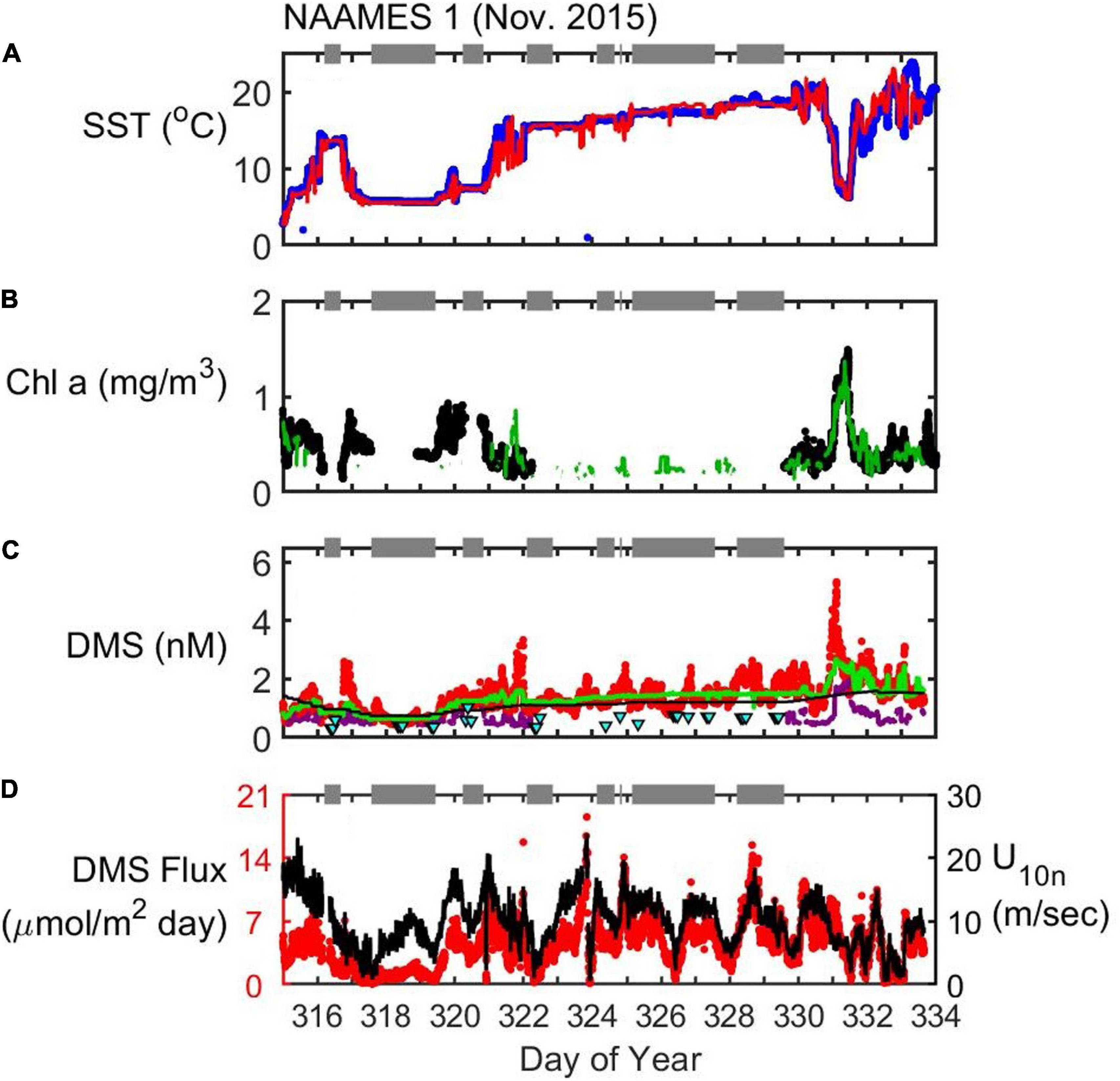
Figure 4. Timeseries of SST (A), Chl (B), seawater DMS (C), and wind speed (U10n)/DMS flux (D) during the NAAMES1 field campaign (November 2015). In situ observations of SST (blue dots) and Chl (black dots) are plotted alongside satellite observations extracted along the cruise track (red and green lines for SST and Chl, respectively). Seawater DMS measurements during the cruise (red dots) are shown alongside data extracted from the Lana et al. (2011) climatology for November (L11, black line), data extracted from neural network model output (green line) and the Galí et al. (2018) estimate (G18, solid purple line). Cyan triangles are the G18 prediction using MLD estimated from in situ CTD (temperature and salinity) profiles. Gaps occur in G18-predicted DMS when there is no available in situ Chl data (e.g., Day of Year 322.2–329.6). Gray bars at the top of each panel indicate periods when the ship was on station. DMS flux (red dots) is calculated from in situ observations of U10n (black line), seawater DMS and SST.
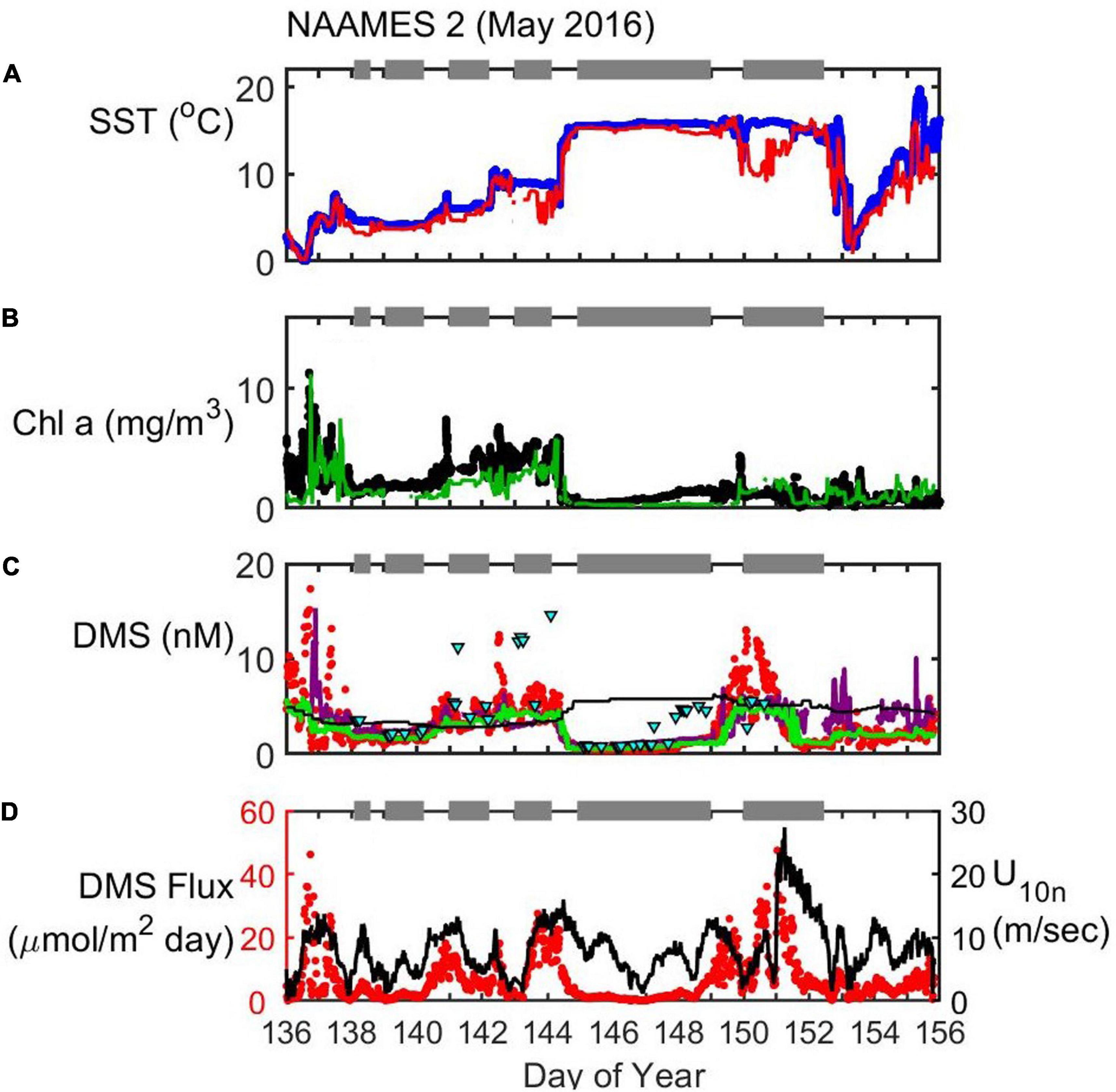
Figure 5. Timeseries of SST (A), Chl (B), seawater DMS (C), and wind speed (U10n)/DMS flux (D) during the NAAMES2 field campaign (May 2016). In situ observations of SST (blue dots) and Chl (black dots) are plotted alongside satellite observations extracted along the cruise track (red and green lines for SST and Chl, respectively). Seawater DMS measurements during the cruise (red dots) are shown alongside data extracted from the Lana et al. (2011) climatology for November (L11, black line), data extracted from neural network model output (green line) and the Galí et al. (2018) estimate (G18, solid purple line). Cyan triangles are the G18 prediction using MLD estimated from in situ CTD (temperature and salinity) profiles. Gray bars at the top of each panel indicate periods when the ship was on station. DMS flux (red dots) is calculated from in situ observations of U10n (black line), seawater DMS and SST.
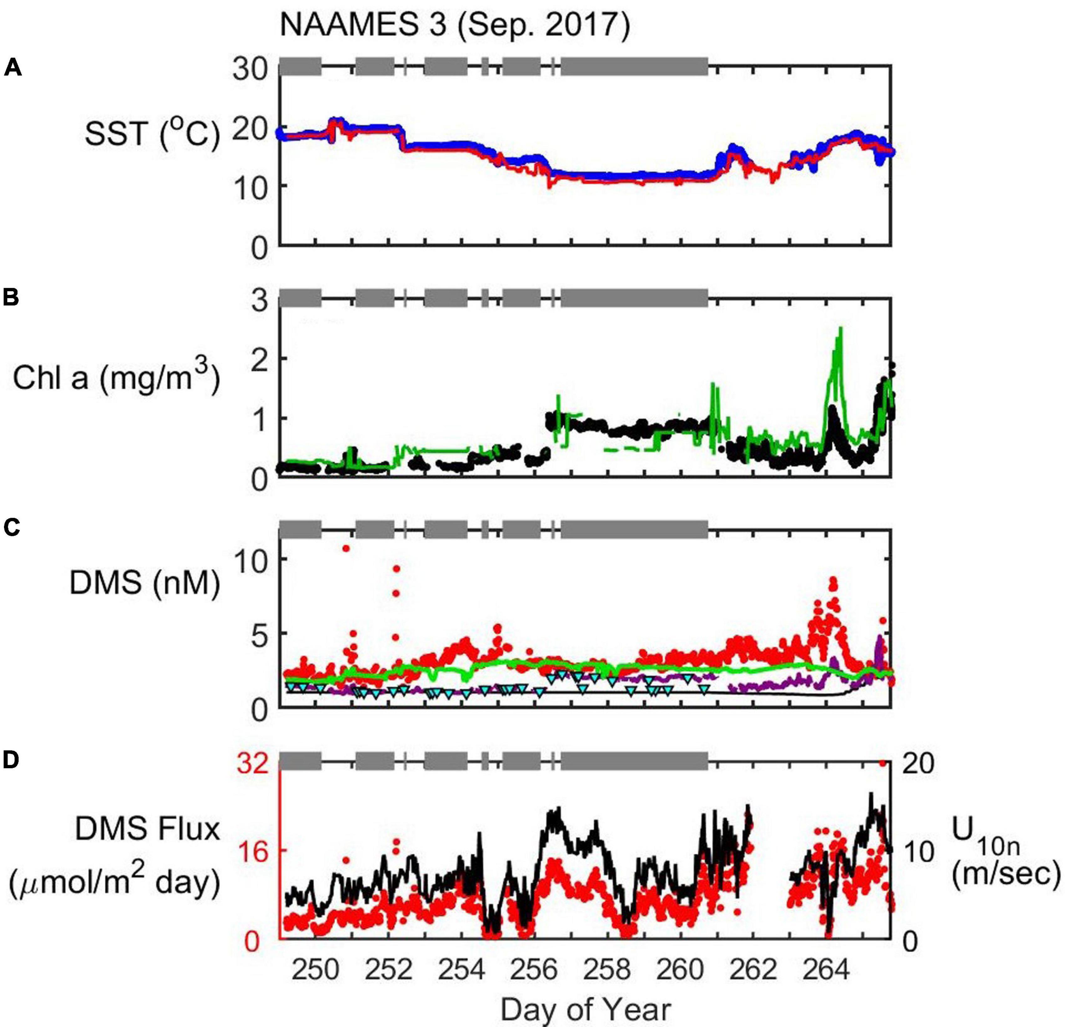
Figure 6. Timeseries of SST (A), Chl (B), seawater DMS (C), and wind speed (U10n)/DMS flux (D) during the NAAMES3 field campaign (September 2017). In situ observations of SST (blue dots) and Chl (black dots) are plotted alongside satellite observations extracted along the cruise track (red and green lines for SST and Chl, respectively). Seawater DMS measurements during the cruise (red dots) are shown alongside data extracted from the Lana et al. (2011) climatology for November (L11, black line), data extracted from neural network model output (green line) and the Galí et al. (2018) estimate (G18, solid purple line). Cyan triangles are the G18 prediction using MLD estimated from in situ CTD (temperature and salinity) profiles. Gray bars at the top of each panel indicate periods when the ship was on station. DMS flux (red dots) is calculated from in situ observations of U10n (black line), seawater DMS and SST.
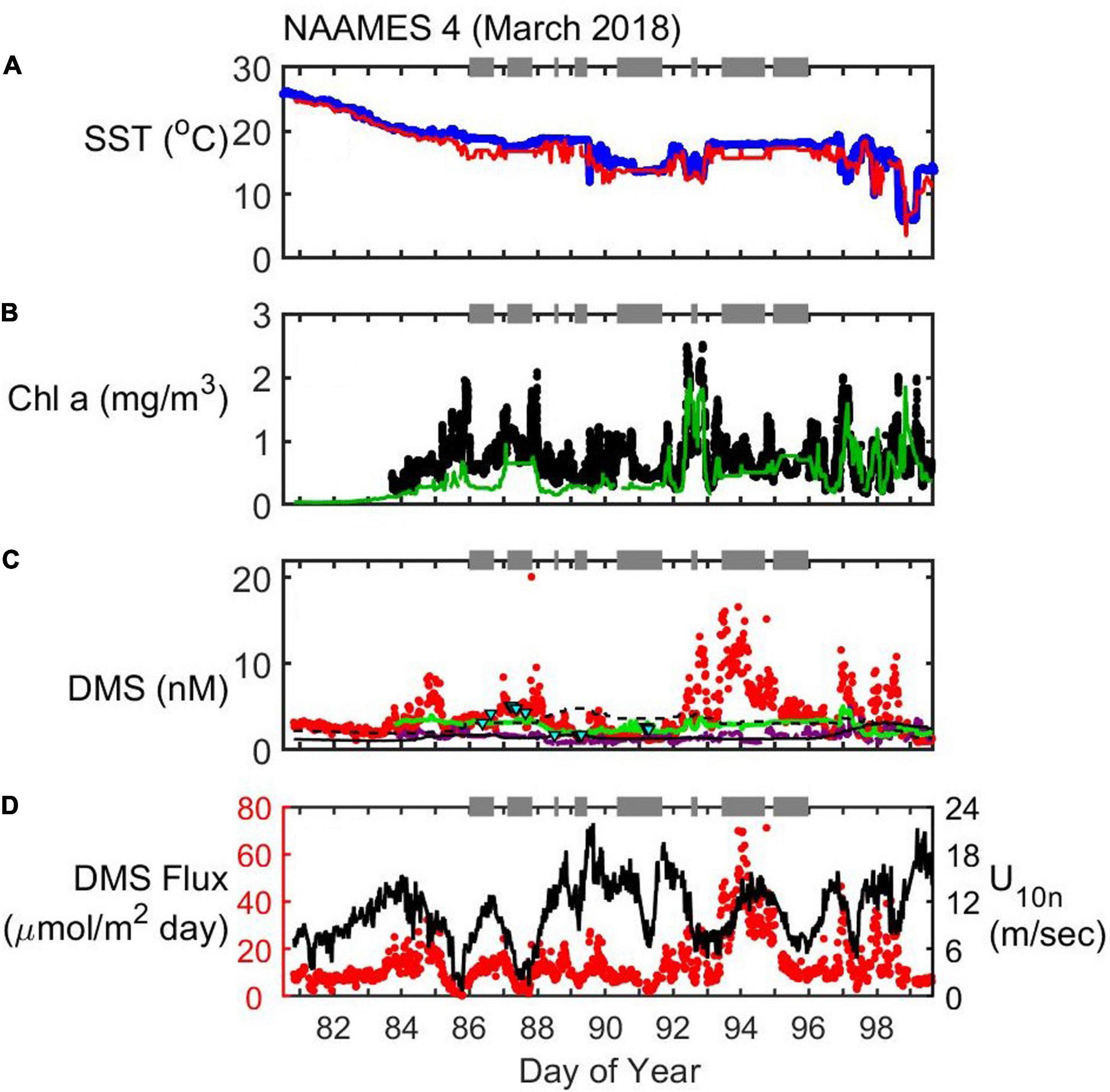
Figure 7. Timeseries of SST (A), Chl (B), seawater DMS (C), and wind speed (U10n)/DMS flux (D) during the NAAMES4 field campaign (March/April 2018). In situ observations of SST (blue dots) and Chl (black dots) are plotted alongside satellite observations extracted along the cruise track (red and green lines for SST and Chl, respectively). Seawater DMS measurements during the cruise (red dots) are shown alongside data extracted from the Lana et al. (2011) climatology for November (L11, black line), data extracted from neural network model output (green line) and the Galí et al. (2018) estimate (G18, solid purple line). Gaps occur in G18-predicted DMS when there is no available in situ Chl data (e.g., prior to Day of Year 83.8). Cyan triangles are the G18 prediction using MLD estimated from in situ CTD (temperature and salinity) profiles. Gray bars at the top of each panel indicate periods when the ship was on station. DMS flux (red dots) is calculated from in situ observations of U10n (black line), seawater DMS and SST.
NAAMES1 (November 2015)
NAAMES1 took place during the early winter transition that initiates the annual phytoplankton bloom (Behrenfeld and Boss, 2014, 2018). The ship stopped to occupy seven stations during the cruise (gray dots in Figure 3, gray bars in Figure 4). The second station was the most northerly (54.1°N, DOY 318) and the last station was the most southerly (40.6°N, DOY 329). The data collected while on station typically show less variability than when the ship was underway. For example, large variations in SST, Chl, and DMS occurred while the ship moved in and out of a region of biologically productive, cold water over ∼21 h (DOY 331; range of 12.5°C, 1.2 mg/m3 and 4.1 nM for SST, Chl, and DMS, respectively). DMS and Chl levels appear to co-vary during the transit into cold waters and back into warm Gulf Stream waters, but the data are only weakly correlated (Spearman’s ρ = 0.32, p < 0.001, n = 168).
Mean DMS concentration was 1.4 nM during NAAMES1, and ranged from 0.4 to 5.3 nM. The variations in seawater DMS occur over relatively small spatial scales and appear to be associated with rapid changes in SST (Figure 4). Variations in surface Chl were sometimes coincident with the DMS changes. For example, DMS increased from 0.75 to 2.6 nM over 40 min on DOY 316.75. SST reduced by 2.9°C over this period and the Chl increased by 0.3 mg/m3. The ship speed was 10.5 knots during the changes in DMS, Chl and SST, corresponding to a distance of ∼13 km. On DOY 322, SST increased rapidly by 4°C and DMS reduced abruptly from 3.4 to 1.0 nM. The change in Chl (−0.2 mg/m3) was not quite as pronounced as on DOY 316.75.
There have been few observations of seawater DMS in the western North Atlantic during November prior to NAAMES1. The L11 climatology uses extrapolation and interpolation of existing data and predicts low levels for the region. The extracted L11 data agree quite well with the seawater DMS observations (Spearman’s ρ = 0.63, p < 0.001, n = 3930; Figure 4C). The L11 data are a climatological product and thus the extracted L11 data do not show a lot of spatial variability. The G18 prediction is spatially variable, but does not fully capture the observed DMS variations and tends to under-predict observed levels. The neural network model output provides a closer approximation to the typical observed DMS concentrations and variability, but tends to underestimate DMS when observed concentrations are elevated (e.g., DOYs 317, 322, and 331).
Wind speed variations had an important influence on the DMS flux during NAAMES1 (Figure 4D). The wind speed during the cruise averaged 9.8 m sec–1 and ranged from close to 0–23.8 m s–1. The calculated flux of DMS into the North Atlantic atmosphere during NAAMES1 ranged from 0.1 to 18.5 μmol m–2 day–1 (NAAMES1 mean flux = 4.4 μmol m–2 day–1).
NAAMES2 (May 2016)
NAAMES2 targeted the climax of the annual phytoplankton bloom. Stations at the northern end of the 40°W transect were targeted at the beginning of the cruise. The second station (S1) was the furthest North (56.3°N, 46.0°W; DOY 139). Measurements made between DOY 136 and 144 (including the first four stations, S0–S3) were in waters with elevated biological activity (mean ± SD Chl = 3.0 ± 1.3 mg/m3) and DMS concentrations (mean ± SD = 3.9 ± 2.7 nM). The latter part of the cruise (after the final station, S5, and during the transit back to Woods Hole) took place in lower latitude waters (<45.1°N). The southern, warmer waters during NAAMES2 were less productive (0.8 ± 0.5 mg/m3) with lower DMS concentrations (2.0 ± 0.8 nM). Rapid changes in DMS associated with rapid SST and Chl changes were sometimes observed during NAAMES2. On DOY 144.4, for example, Chl and DMS reduced by 3.6 mg/m3 and 4.9 Nm, respectively, as the SST increased rapidly from 6.6 to 13.4°C.
The effect of wind-driven mixing on surface Chl and DMS levels is particularly evident in the NAAMES2 data. Station S4 (DOY 145) was targeted because it had recently experienced an intense wind-driven mixing event. The surface layer had been mixed to ∼250 m and this diluted the near-surface with low concentration sub-surface waters (Graff and Behrenfeld, 2018). The mixed layer dilution coupled with the sea-to-air loss of DMS resulted in surface concentrations of Chl (0.4 mg/m3) and DMS (0.6 nM) that were low for the time of year. Calm conditions persisted during the occupation of S4 and the mixed layer shallowed to < 30 m after 3 days. A shallower MLD coincided with a gradual increase in Chl up to 1.5 mg/m3 by DOY 149. The DMS response was slower than the Chl response, but DMS levels had increased to 1.7 nM by DOY 149 when the ship left station. A large, Eastward-moving storm (wind speeds up to ∼25 m sec–1) affected the final station (S5; 44.4°N, 43.4°W). DMS levels during S5 were 11.6 nM on DOY 150.5 but rapidly reduced to 1.0 nM during the storm on DOY 152.4.
The extracted L11 data are typically in good agreement with in situ observations during the first half of the cruise (mean DMS: L11 = 3.3 nM, observed = 3.9 nM; Figure 5). The agreement between in situ and L11 data worsens in the second half of the cruise when storms reduced the in situ DMS concentrations (mean DMS: L11 = 5.2 nM, observed = 2.2 nM). Storms encourage ventilation to the atmosphere and deepen the MLD, reducing light exposure, diluting near-surface concentrations and potentially transporting DMS-producing organisms below the photic zone.
The increase in DMS throughout DOYs 145–149 is relatively well-predicted by the G18 algorithm, which responds to the increase in biomass during this period (Spearman’s ρ = 0.67, p < 0.001, n = 248; Figure 5). The in situ MLD shallowed to 30 m on DOY 148 and this change is not reflected in the Argo MLD (Supplementary Figure S2). The sensitivity of the G18 prediction to MLD is highlighted by the contrast between predictions made using in situ CTD MLD estimates vs. predictions made using monthly averaged Argo MLD (Figure 5). The G18 estimate using the climatological Argo MLD makes a better prediction of in situ DMS than if the in situ MLD was used (Figure 5).
The neural network model predictions throughout NAAMES2 are similar to the G18 predictions (Figure 5). The DMS prediction by the neural network model responds to the change in biomass during DOYs 145–149 and effectively captures the variability (Spearman’s ρ = 0.69, p < 0.001, n = 248; Figure 5). Neither of the predictions from G18 and the neural network are accurate on DOY 150, both underestimating in situ DMS levels by as much as 50%. After the storm passed over the ship during station S5, DMS levels were over-estimated by the G18 algorithm. G18 continued to over-predict DMS while the ship traveled West through storm-influenced waters (until approximately DOY 155). The neural network DMS prediction was lower than the G18 estimate during DOYs 152–155, and in better agreement with the observed DMS levels.
The average wind speed during NAAMES2 (U10n mean = 8.2 m s–1) was lower than NAAMES1 although the large storm on DOY 151 resulted in the strongest winds observed during all NAAMES cruises (U10n max. = 27.4 m s–1). The variation in DMS concentrations was large (from 0.4 to 17.4 nM) and had an important influence on the variability and magnitude of the calculated DMS flux (0.1–47.5 μmol m–2 day–1; Figure 5). The mean flux of DMS into the North Atlantic atmosphere during NAAMES2 is calculated as 6.6 μmol m–2 day–1.
NAAMES3 (September 2017)
NAAMES3 took place during the declining phase of the phytoplankton bloom (Behrenfeld and Boss, 2014, 2018). The 40°W transect began at the southern-most extent and headed North. The first three Stations (S1a, S1, and S1.5) were not sampled for DMS due to instrument problems. DMS measurements began at 44.4°N (during Station S2, DOY 249). Six additional stations were briefly occupied and the final and most northerly station (S6, 53.4°N) was occupied for 4 days. The ship returned to Woods Hole following a route that was relatively close to the coast to avoid the heavy seas associated with Hurricane José (see Behrenfeld et al., 2019). Instrument problems and the return transit close to the coast meant that warmer North Atlantic waters were not sampled for seawater DMS. The maximum SST encountered while measuring seawater DMS was 20.9°C, in contrast to when the ship was South of S2 (maximum SST = 28.0°C).
A range in Chl was encountered during the seawater DMS measurement period of NAAMES3 (DOY 249–266). Station S2 Chl (0.2 mg/m3) was lower than Chl during the northern Station S6 (0.9 mg/m3). The majority of in situ and MODIS Chl data compare well during all the NAAMES cruises. However, in situ Chl data are notably lower than the MODIS Chl retrieval on DOY 264 (Figure 6B). The disagreement between in situ and MODIS Chl occurred as the ship passed through a phytoplankton bloom on the return leg to Woods Hole (Figure 3C, 45.5°N, 58.0°W). The MODIS and in situ Chl levels both increase and decrease as the ship moves in and out of the bloom (Figure 6B). The most likely explanation for the difference is that the ship arrived at the bloom location after the peak in biomass and missed the high Chl levels captured by the monthly MODIS data product.
The average seawater DMS during NAAMES3 (mean ± SD = 3.1 ± 1.0 nM; Figure 6C) was substantially higher than either the extracted L11 data (1.2 ± 0.5 nM) or the G18 prediction (1.7 ± 0.5 nM). In situ SST did not change rapidly during NAAMES3 (Figure 6A) and DMS variability cannot easily be linked to SST fronts (as was possible during NAAMES1 and NAAMES2). Seawater DMS did not show a lot of variability during the cruise, with the exception of the bloom encountered on DOY 264 (Figure 6C). In situ DMS levels increased to 8.6 nM in the center of the bloom on DOY 264. The G18 algorithm also predicts increased DMS, but with a maximum of only 3.3 nM. G18 predictions throughout NAAMES3 were similar irrespective of the choice of in situ MLD or Argo climatological MLD.
DMS predicted by the neural network model is higher than the L11 or the G18 prediction. The neural network model DMS and in situ DMS observations during the cruise are comparable, but the neural network model mean (2.6 nM) is lower than the observations (3.2 nM) mainly because the model poorly represents the periods when DMS is elevated. The neural network model fails to predict the elevated DMS levels on DOY 254 and in particular the high DMS associated with the phytoplankton bloom on DOY 264 (Figure 6C). The neural network model and G18 estimates both under-predict observed DMS on DOY 264 by a similar magnitude (∼5 nM).
The majority of the variability in calculated DMS flux during NAAMES3 is driven by variations in wind speed because seawater DMS did not vary substantially (mean ± SD = 3.2 ± 1.0 nM; Figures 6C,D). Wind speed ranged from 0.6 to 16.5 m s–1 (mean U10n = 7.6 m s–1) with peak wind speeds driving the peak DMS fluxes. NAAMES3 DMS fluxes ranged from 0.4 to 31.6 μmol m–2 day–1 (mean = 7.5 μmol m–2 day–1).
NAAMES4 (March/April 2018)
NAAMES4 took place during the accumulation phase of the phytoplankton bloom (Behrenfeld and Boss, 2014, 2018). As previously discussed, the cold, productive waters at the northern end of the 40°W transect were not sampled because the ship departed from Puerto Rico and storms restricted sampling at higher latitudes. The highest latitude station was S4 (DOY 91; 44.5°N). SST did not vary a lot (mean ± SD SST = 18.5 ± 5.7°C) with few oceanic temperature fronts (i.e., rapid SST changes). Eight stations were sampled during NAAMES4, but only Station SE4 (DOY 92.5) sampled an eddy (Della Penna and Gaube, 2019).
Chl was quite variable during NAAMES4 (0.7 ± 0.4 mg/m3), with lots of spikes that do not correspond to changes in SST (Figures 7A,B). There were fewer spikes in DMS than in Chl, particularly during the first half of the cruise when DMS levels were lower (mean ± SD DMS prior to DOY 92 = 3.0 ± 1.5 nM). The ship moved through waters that were more biologically productive after DOY 92. DMS levels were higher and more variable after DOY 92 (mean ± SD DMS = 5.0 ± 3.3 nM; Figure 7C) and this coincided with a region containing greater variability in sea surface height anomaly (Figure 8A). A high Chl feature was sampled inside a cyclonic eddy before, during, and after Station SE4 (DOY 92.5, Figure 8B). DMS and Chl co-varied within the cyclonic eddy, with elevated DMS when Chl concentrations were high (max. Chl = 2.5 mg/m3 and max. DMS = 13.2 nM; Figure 8C). Note that there were also periods during NAAMES4 when elevated DMS levels did not correspond to high Chl levels (e.g., DOY 93.5 during Station S2RD: DMS = 13.7 nM; Chl = 0.7 mg/m3).
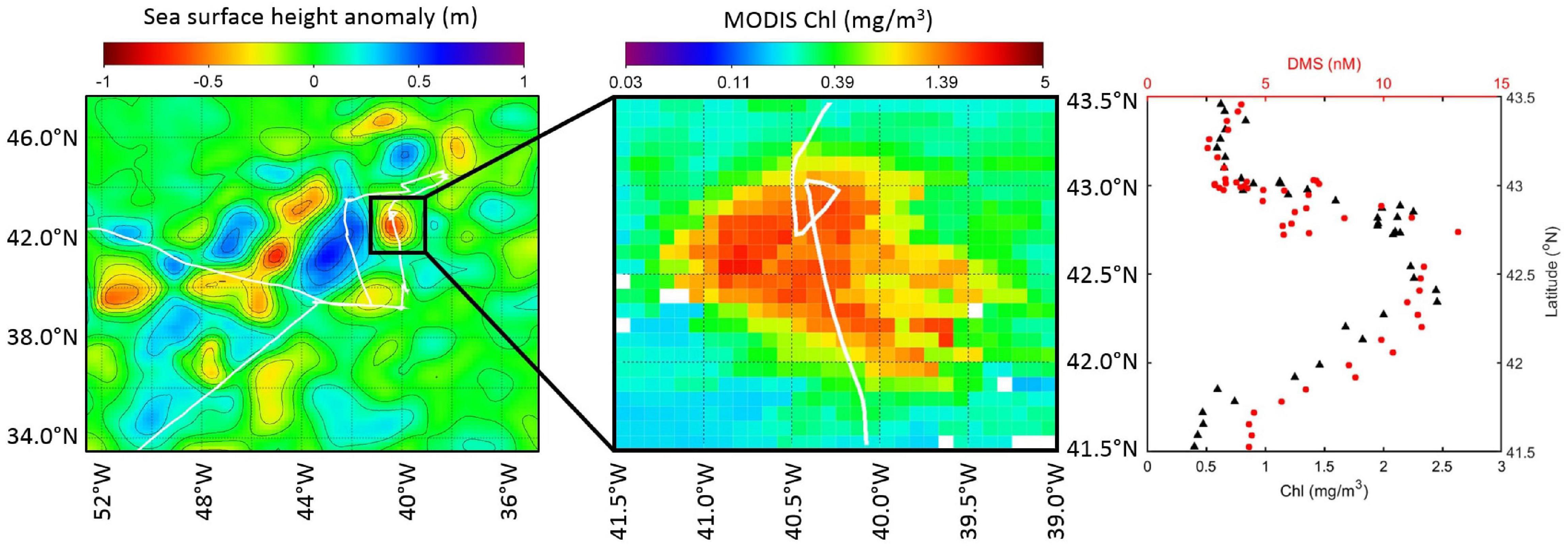
Figure 8. High Chl feature within a cyclonic eddy targeted on DOY 92.5 during NAAMES4 (Station SE4). Cruise track is shown in white. Left panel: Gridded sea surface height anomaly derived from radar altimeter measurements. Middle panel: MODIS Chl spatial distribution within the eddy. Right panel: Latitudinal variation in in situ Chl and DMS within the eddy.
DMS estimates from the extracted L11, neural network model and G18 algorithm are consistently lower than the observed DMS levels, particularly during the latter half of the cruise (DOY 92 onwards; Figure 7C). The G18 DMS prediction improves when in situ CTD MLD can be used (DOY 86–92) instead of climatological Argo MLD. There was no significant correlation between the Argo MLD climatology and MLD from in situ CTD profiles during NAAMES4, whereas there was a moderate correlation for NAAMES1–3 (Spearman’s ρ = 0.37, p < 0.001, n = 106; see Supplementary Figures S1, S2). A winch failure during NAAMES4 (Behrenfeld et al., 2019) meant that CTD profiles were unfortunately only collected prior to DOY 92. The Argo-based G18 prediction and the neural network model underestimate the observed DMS concentrations by up to 15 nM during DOY 92–95. The period of substantial DMS underestimation includes stations with high Chl (Station SE4, DOY 92.5: high Chl, cyclonic eddy, Figure 8) and low Chl (Station S2RD, DOY 93.5). It is not possible to determine whether using in situ MLDs would have substantially improved the G18 and neural network estimates of seawater DMS during this period.
NAAMES4 encountered higher wind speeds on average compared to the other NAAMES cruises (mean U10n = 10.7 m s–1). Winds blew consistently throughout NAAMES4 and, when combined with elevated seawater DMS levels in the latter half of the cruise, resulted in the highest average DMS flux to the atmosphere of all NAAMES cruises (mean = 13.7 μmol m–2 day–1). Variability in DMS concentration (range = 0.9–20.1 nM) dominated the variability in calculated DMS flux (range = 0.3–71.1 μmol m–2 day–1; Figure 7D).
Seasonal Variability in Chl and DMS
The NAAMES cruises span 4 years (2015–2018 inclusive), but can be used to represent the stages of the seasonal phytoplankton bloom over a virtual year (i.e., November → March/April → May → September). The seasonal variation in Chl and DMS is evident when the data are summarized with box and whisker plots (Figure 9). The waters encountered during the NAAMES field campaigns contained similar Chl distributions (mean, median, range and distribution shape) as the MODIS distribution extracted from the wider North Atlantic region (Figure 9A). The similarities between along-track MODIS Chl and regional North Atlantic MODIS Chl suggests that any insight gained from the NAAMES data could be applied to the wider region. Note that alternative measures of the biological community may not show the same spatial and temporal patterns as the Chl, and this is a caveat to any large scale interpretation of the NAAMES data.
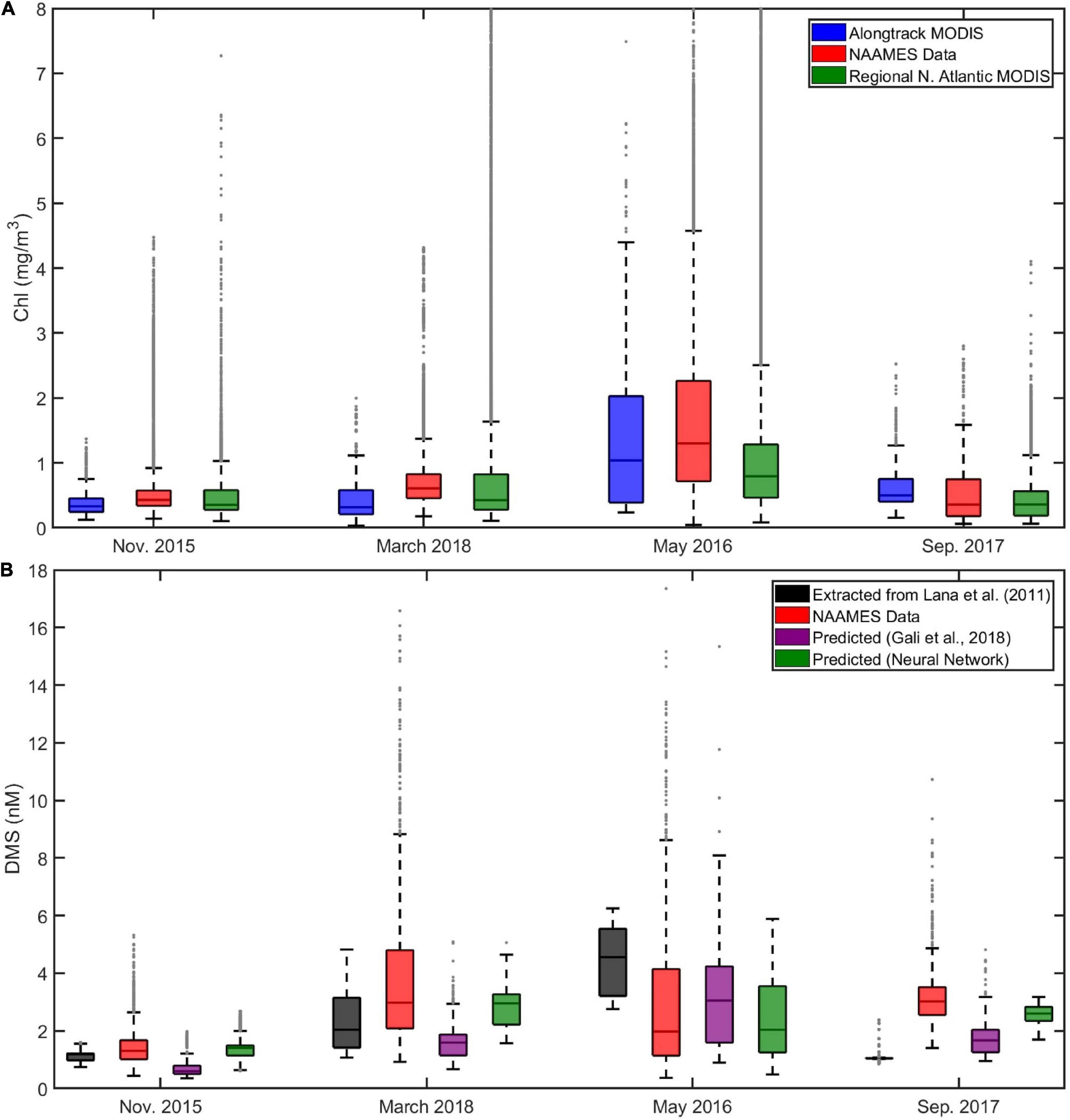
Figure 9. Box and whisker summary of seawater Chl (A) and DMS (B) during the NAAMES cruises (Nov., 2015, NAAMES1; March/April 2018, NAAMES4; May 2016, NAAMES2; September 2017, NAAMES3). The central horizontal line on each box is the median, and the bottom and top edges of the box indicate the 25th and 75th percentiles, respectively. The whiskers extend to the most extreme data points not considered outliers. Outliers (gray dots) are identified as data that is > 1.5 times the interquartile range above the top or below the bottom of the box. The data are presented in an order that highlights the seasonal changes in North Atlantic seawater Chl and DMS (winter through to fall) rather than the chronological order in which the cruises were conducted. In situ NAAMES data are shown in red. Additional plots in (A) are the MODIS Chl data extracted along the cruise track (blue) and from the wider North Atlantic (region limits defined in the text, green). The Y-axis scale has been limited to 8 mg/m3 for clarity. Additional plots in (B) are the DMS data extracted from the Lana et al. (2011) climatology (L11, black), the Galí et al. (2018) prediction (G18, purple) and the artificial neural network prediction (green).
Box and whisker plots provide an overview comparison between DMS observations, extracted L11, and the G18 and neural network model output (Figure 9B). Cruises in March and May encountered DMS concentrations that were higher than the November cruise. Seawater DMS levels during the late summer cruise (September) were also higher than the winter observations, and higher than predicted by either L11 or G18 (Figure 9B). The neural network model did fairly well at predicting the average seasonal cycle in DMS.
The seawater DMS measurements from each NAAMES cruise have a strong skew with a positive tail (i.e., the infrequent occurrence of higher DMS concentrations, Figure 9B). None of the L11, G18 and neural network predictions of DMS have distributions with as strong a skew as the in situ observations. For example, G18-predicted and observed DMS in May are similar in the mean (3.1 and 2.9 nM, respectively), but the skew in the observed data is highlighted by the substantially different median values (G18 = 3.1 nM; observed DMS = 2.0 nM).
The extracted L11 does a particularly poor job at representing the NAAMES DMS data distribution/shape (Figure 9B). The extracted L11 data have a normal distribution, which is in sharp contrast to the skewed distribution of the in situ observations. The characteristics of the L11 data highlight the techniques used to generate the DMS climatology. L11 sorted the DMS database into monthly sub-datasets, calculated the average (mean), then interpolated and smoothed over large spatial scales to produce a seasonal climatology with continuous spatial coverage.
Spatial Variability in Seawater DMS
Spatial variability in seawater DMS predicted by L11, G18, and the neural network model highlights the differences between estimates of DMS in the North Atlantic (Figures 10–13). The spatial variation in the L11 climatological DMS is substantially lower than the G18 and neural network climatologies. All three DMS estimates share some common features such as elevated DMS levels in March in waters southeast of Newfoundland, Canada (Figure 11). Elevated DMS in Atlantic waters North of 40°N in May are predicted by all three climatologies, although the spatial extent of the high DMS region in the L11 climatology is much bigger (Figure 12). Elevated DMS levels in other waters and/or months are only predicted by one or two of the climatologies. For example, the G18 and neural network climatologies predict a large swathe of elevated DMS (> 2 nM) in low latitude waters in March, whereas the L11 does not (Figure 11). The L11 and neural network climatologies predict DMS > 2 nM in low latitude waters in September, whereas the G18 estimate is lower (Figure 13).
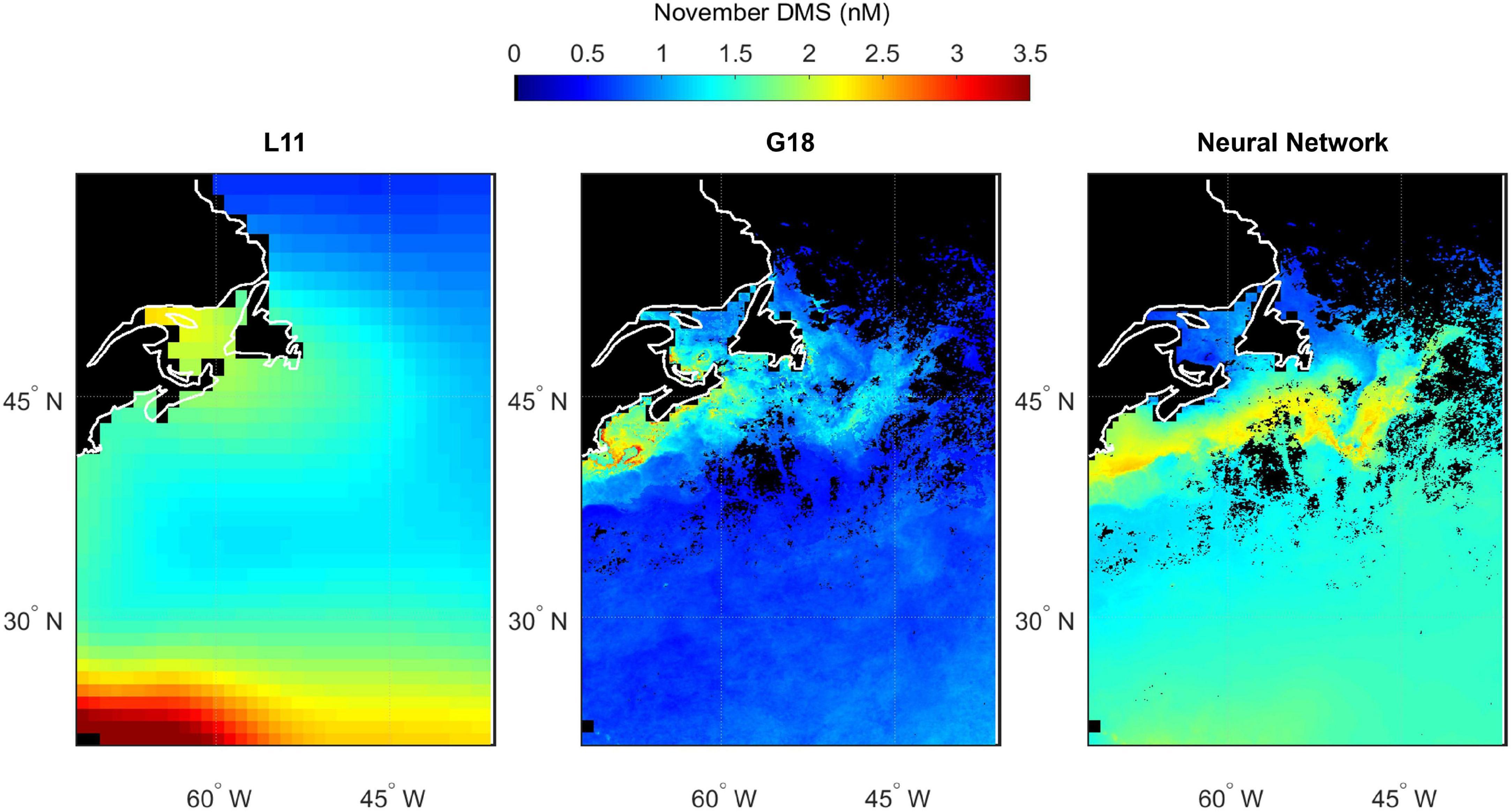
Figure 10. Predicted spatial distribution of seawater DMS in the North Atlantic during November. Climatological maps are extracted from Lana (L11, left panel), the Galí et al. (2018) prediction (G18, middle panel) and the neural network model prediction (right panel). G18 and the neural network output are specific to the NAAMES1 field campaign period because they use MODIS Chl and SST from November 2015, whereas L11 is not specific to a certain year. Scales are capped at 3.5 nM to maintain spatial contrast and aid comparability between panels. Some L11 data exceed the cap (maximum value of 4.2 nM). Pixels with no data/land are filled black.
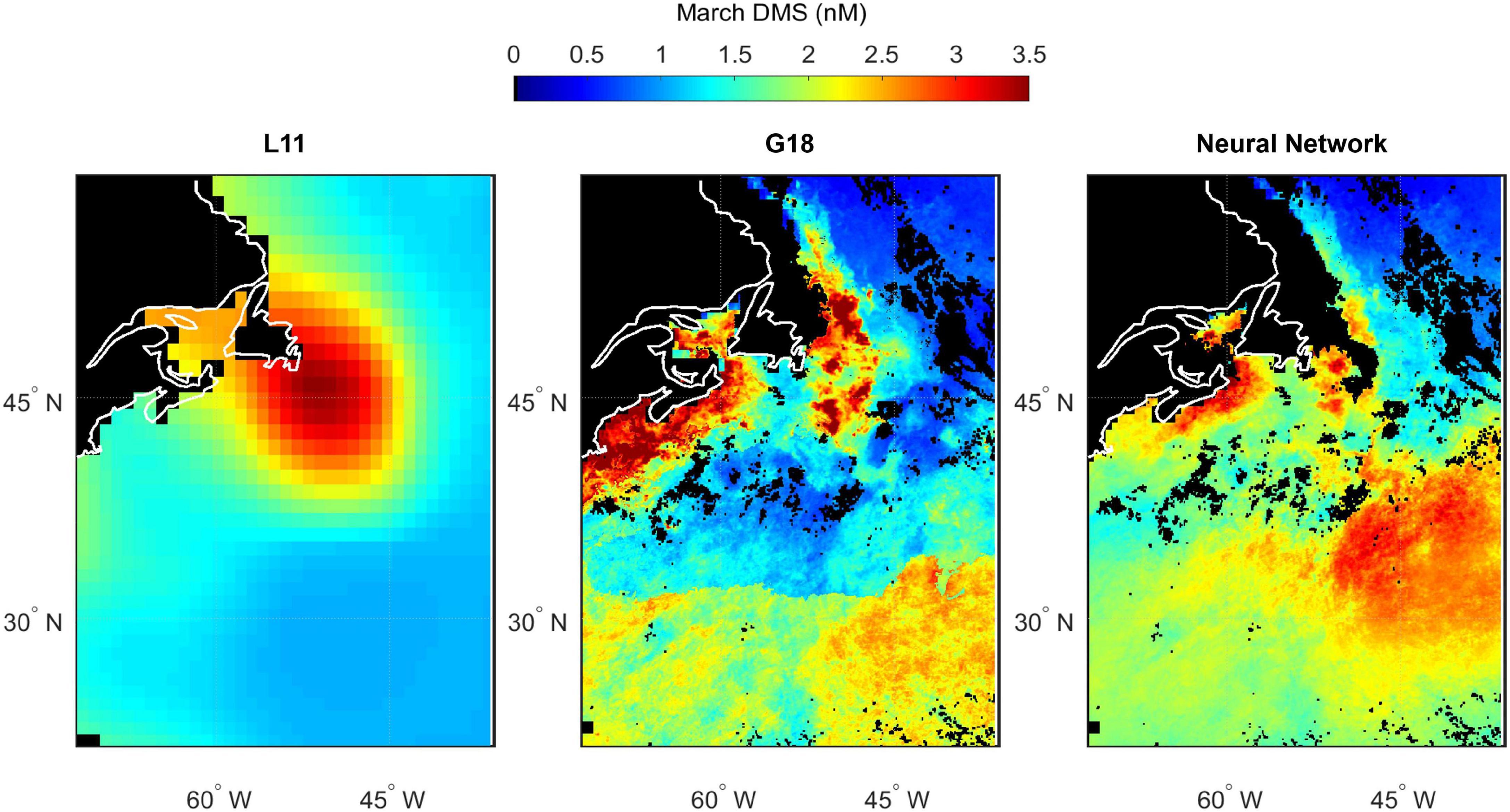
Figure 11. Predicted spatial distribution of seawater DMS in the North Atlantic during March. Climatological maps are extracted from Lana (L11, left panel), the Galí et al. (2018) prediction (G18, middle panel) and the neural network model prediction (right panel). G18 and the neural network output are specific to the NAAMES4 field campaign period because they use MODIS Chl and SST from March/April 2018, whereas L11 is not specific to a certain year. Scales are capped at 3.5 nM to maintain spatial contrast and aid comparability between panels. Some G18 and W20 data exceed the cap (maximum values of 7.2 and 5.0 nM respectively). Pixels with no data/land are filled black.
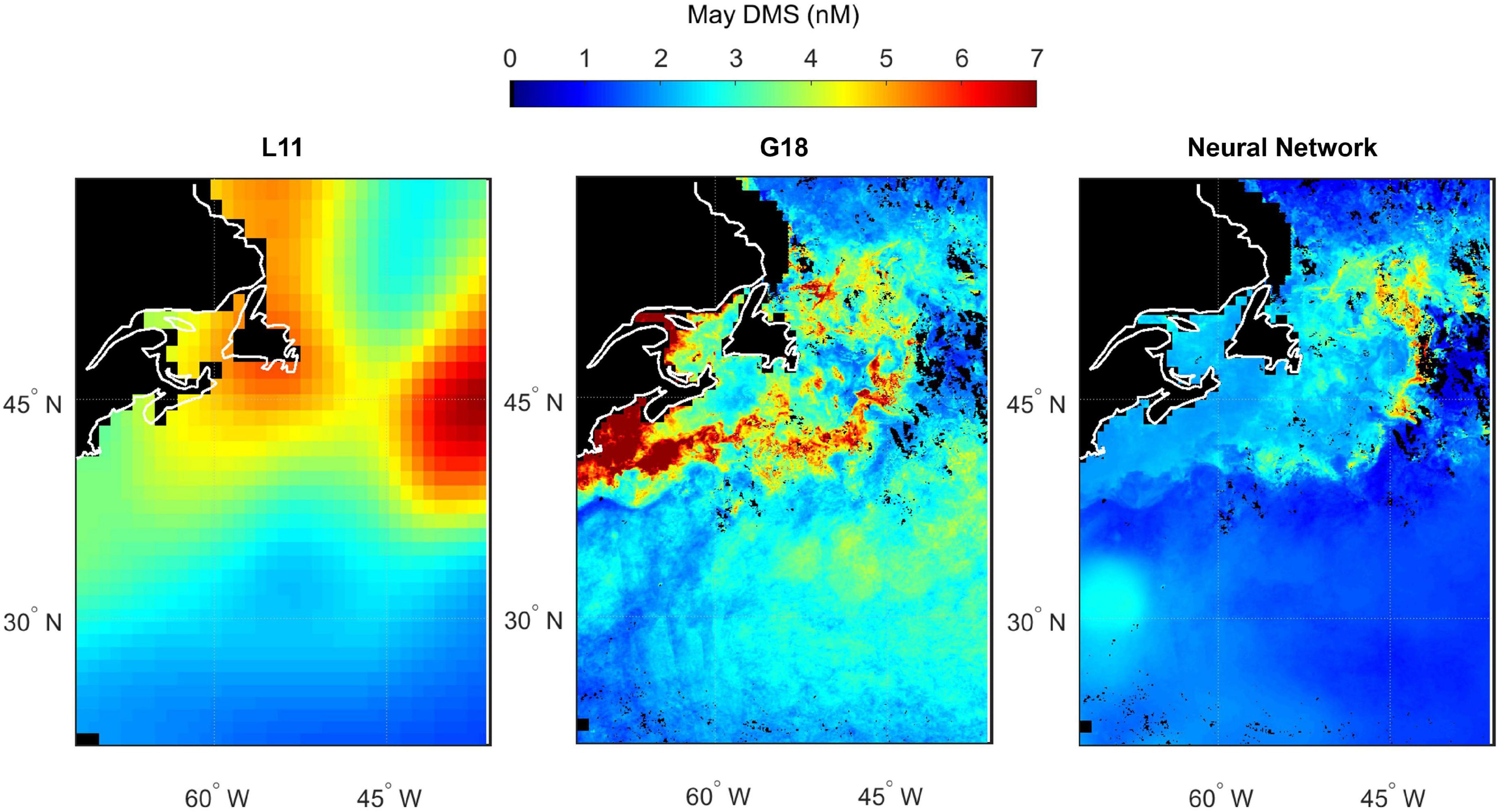
Figure 12. Predicted spatial distribution of seawater DMS in the North Atlantic during May. Climatological maps are extracted from Lana (L11, left panel), the Galí et al. (2018) prediction (G18, middle panel) and the neural network model prediction (right panel). G18 and the neural network output are specific to the NAAMES2 field campaign period because they use MODIS Chl and SST from May 2016, whereas L11 is not specific to a certain year. Scales are capped at 7.0 nM to maintain spatial contrast and aid comparability between panels. Some G18 data exceed the cap (maximum value of 38.5 nM). Pixels with no data/land are filled black.
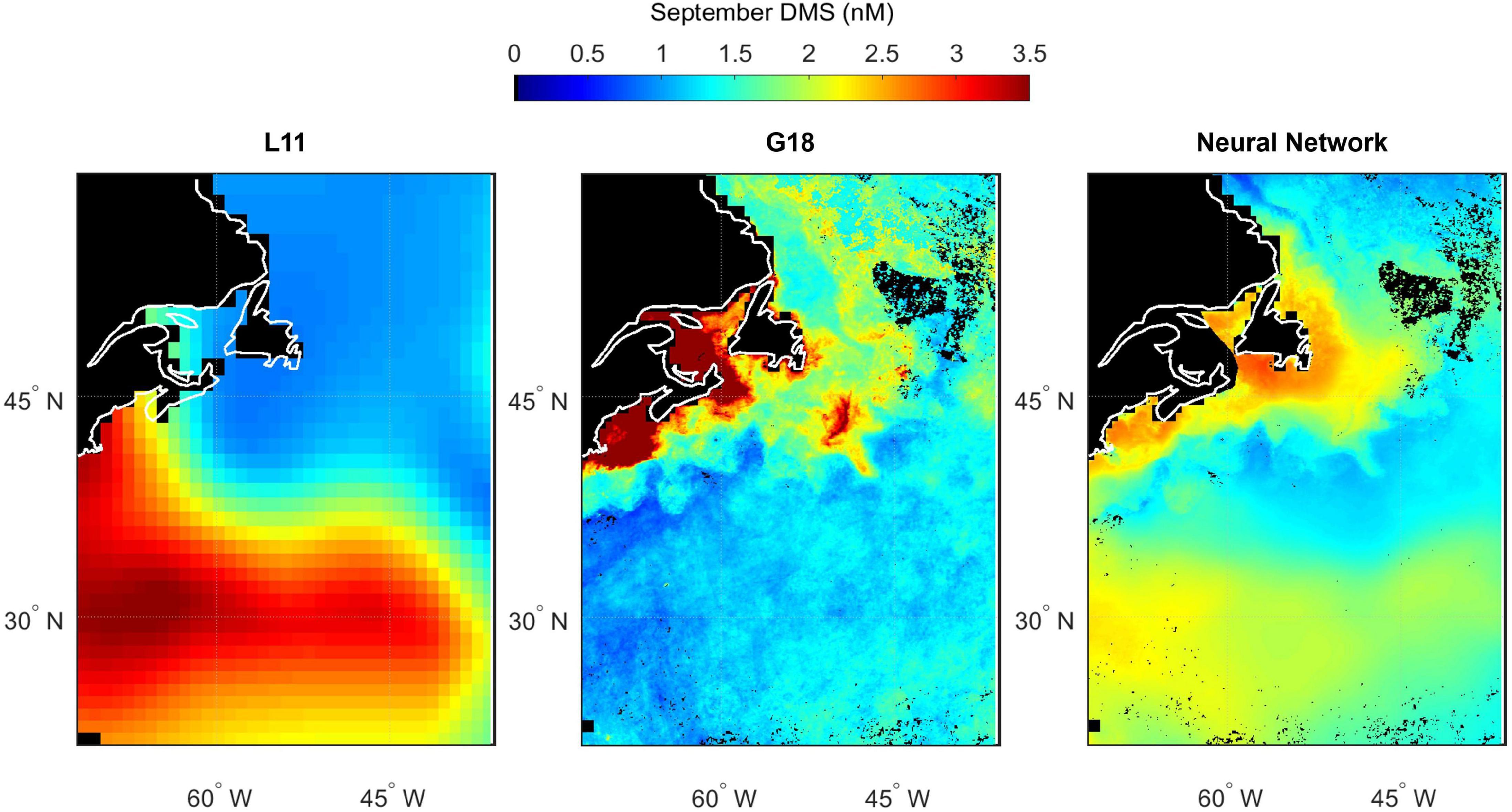
Figure 13. Predicted spatial distribution of seawater DMS in the North Atlantic during September. Climatological maps are extracted from Lana (L11, left panel), the Galí et al. (2018) prediction (G18, middle panel) and the neural network model prediction (right panel). G18 and the neural network output are specific to the NAAMES3 field campaign period because they use MODIS Chl and SST from September 2017, whereas L11 is not specific to a certain year. Scales are capped at 3.5 nM to maintain spatial contrast and aid comparability between panels. Some G18 data exceed the cap (maximum value of 29.2 nM). Pixels with no data/land are filled black.
The input parameters common to the G18 algorithm and neural network model are Chl, SST, PAR, and MLD. The G18 and neural network DMS plots contain features that appear like the ocean (fronts, eddies, etc.). The “oceanic DMS features” are generated by spatial variations in MODIS Chl and SST (Figures 2, 3). A climatological average product was used for MLD and for PAR. The relative sensitivity of the G18 and neural network model estimates to the inputs of Chl and SST is evident when comparing certain regions. For example, the neural network model predicts higher DMS levels in the Gulf Stream in November 2015 than the G18 estimate (Figure 10). The G18 estimate in May 2016 for the same region is higher than the neural network model (Figure 12). The G18 parameterization tends to produce high DMS estimates close to the coast where Chl levels are high, with maximum predictions in May and September of 38.5 and 29.2 nM, respectively (Figures 12, 13).
Observed DMS is consistently under-predicted by the G18 algorithm and neural network model (Figure 14). The G18-predicted average (mean) for November, March/April and September plot below the 1:1 line (Figure 14A). Some of the differences between G18-predicted and observed DMS may be driven by an imperfect estimation of the MLD, although in situ MLDs, and climatological Argo MLD compare well for November and September (Supplementary Figures S1, S2). G18-predicted DMS and observed DMS in May agree well on average (Figure 14A), but this is due to both under and over-prediction at different stages of the cruise. The neural network model under-predicts seawater DMS for all four cruises (Figure 14B), but the agreement with observations is substantially better than the G18 prediction (G18 R2 = 0.17; neural network model R2 = 0.58).
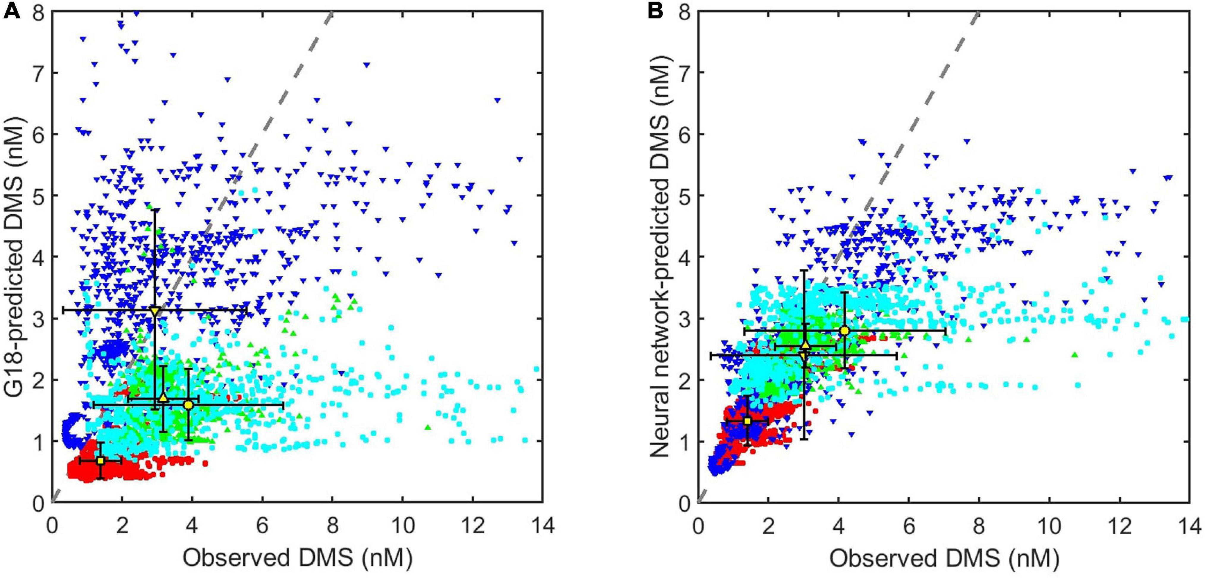
Figure 14. Comparison between observed and predicted seawater DMS concentrations during all four NAAMES cruises (red = November, NAAMES1; cyan circles = March/April, NAAMES4; blue downward triangles = May, NAAMES2; green upward triangles = September, NAAMES3). Mean and uncertainty (error bars are ± 1 SD) DMS for each cruise are identified in yellow (square = November; circle = March/April; downward triangle = May; upward triangle = September). The 1:1 line (dashed gray line) is shown for reference. X and Y-axis limits have been adjusted slightly to maximize clarity, which has resulted in the exclusion of a small number of outlying data points (Figure 9b shows the full extent of the data). DMS predicted by (A) the G18 algorithm (Galí et al., 2018) and (B) a neural network model.
Discussion
The NAAMES DMS data illustrate the interplay of physical and biological forcing on the reduced sulfur cycle in seawater. The qualitative association between DMS and Chl during NAAMES is clear, but the statistical correlation is weak (Spearman’s ρ = 0.32, p < 0.001, n = 4,374) and very little DMS variability is explained by Chl (R2 = 0.15). Physical processes confound the links between DMS and biology, but the correlation of DMS with parameters such as SST and MLD is also weak (DMS vs. SST: Spearman’s ρ = 0.21, p < 0.001, n = 7,043, R2 = 0.004; DMS vs. MLD: Spearman’s ρ = −0.30, p < 0.001, n = 7,061, R2 = 0.02). Elevated surface water DMS are rapidly reduced when the MLD is deepened by wind-driven mixing (e.g., the NAAMES2 high wind speed event on DOY 150, Station S5). Low DMS levels observed on DOY 145 and DOY 152 during the annual bloom climax (NAAMES2, Figure 5) are good examples of how storms can impact DMS levels during a period of the year typically associated with enhanced biological production/DMS. DMS levels are low during the November cruise, with variability associated with frontal variations in SST and Chl (e.g., DOY 322, NAAMES1, Figure 4). The same phenomena is observed during the accumulation phase of the bloom when Chl levels in the North Atlantic are much higher (DOY 92.5, NAAMES4, Figure 7).
The cyclonic eddy sampled in March 2018 during NAAMES4 (Figure 8) is a good example of how environmental conditions can occasionally be conducive to a predictable relationship between DMS and Chl. The conditions that influence the biological community are relatively stable within an eddy. Eddy circulation limits lateral mixing of the phytoplankton community with surrounding waters. Eddy circulation is also an important factor for the depth of the mixed layer. Mixed layer stratification influences the upwelling of sub-surface waters and the supply of nutrients. Pigment analysis suggests that the dominant phytoplankton within the NAAMES4 eddy were the haptophyte group (Kramer et al., 2020). Haptophytes produce a lot of DMS and DMSP relative to other phytoplankton groups (Stefels et al., 2007). It is likely that DMS and Chl levels co-varied because haptophyte biomass and DMS production changed in proportion to the changes in total Chl. DMS levels inside the eddy were high relative to the rest of the March cruise (>10.0 nM at the eddy center, compared to the NAAMES4 mean DMS = 3.9 nM). The NAAMES4 eddy had a retentive surface area of ∼5,000 km2 according to Della Penna and Gaube (2019). The eddy was a substantive feature in the NAAMES study region and features such as this will have a strong influence on the spatial distribution of DMS and make a significant contribution to regional DMS production.
The L11 data are extracted from a smoothed, monthly product and cannot reproduce the observed spatial variability during the NAAMES cruises (Figures 4–7). The L11 climatology infers high seawater DMS concentrations in certain areas of the North Atlantic throughout the year, which does not agree with the predictions from the neural network model or the G18 algorithm (Figures 10–13, also discussed in Galí et al., 2018). The L11 climatology has been invaluable to Earth System modelers, but is ultimately unable to provide a realistic spatial representation of seawater DMS. The L11 climatology is unable to capture DMS spatial variability across ocean temperature fronts in winter, across large mesoscale features such as eddies, or due to short term temporal variability in MLD (e.g., recovery from a strong wind event). The climatological DMS plots predicted by the G18 algorithm and the neural network model clearly demonstrate the impact that using in situ or remotely sensed data (MODIS Chl, SST) would have upon our understanding of spatial variability in seawater DMS (Figures 10–13). The G18 algorithm and neural network model have similar input variables. The differences between the spatial distribution of the G18 and neural network model outputs demonstrate the relative sensitivities that the predictions have to the input variables. The DMS climatologies (Figures 10–13) and SST fields (Figures 2A–D) were used to calculate the sea-to-air DMS flux. The flux calculation uses the mean wind speed from each cruise. The total North Atlantic regional flux estimates can be compared in Table 1. The impact of choosing different climatologies to calculate the DMS flux into the atmosphere is large.
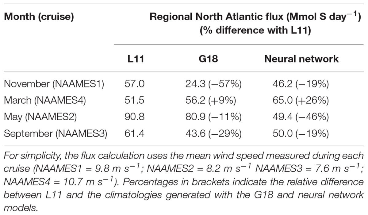
Table 1. Total sea-to-air flux of DMS (Mmol S day–1) in the North Atlantic region (20°–57°N, 72°–38°W) as estimated using the L11 climatology and the G18 and neural network models.
The links between biology and physics are key within many algorithms that use MLD and Chl to predict DMS (e.g., Simó and Dachs, 2002; Vallina and Simó, 2007; Galí et al., 2018). Chl and MLD are also key input variables to the neural network model for DMS presented by Wang et al. (2020). The G18 algorithm and neural network model attempt to resolve DMS variability due to the collective impact of biological and physical processes. An accurate predictive approach coupled with Earth Observation data has enormous potential (Galí et al., 2019). Accurate MLD and Chl are necessary for an accurate prediction, which is highlighted by the difference between the NAAMES4 G18 predictions using in situ MLD vs. climatological MLD.
The neural network model and G18-prediction consistently underestimate the NAAMES in situ DMS data. The underestimation of DMS by these models may be because they were developed using climatological input parameters, which inevitably smooth out the episodic extremes in the predictor variables (Wang et al., 2020). Alternatively, additional parameters may be needed to improve predictive capability. The G18-prediction and neural network model do not explicitly include biological processes that are important in the oceanic reduced sulfur cycle (Stefels et al., 2007): (i) the influence of phytoplankton species composition on DMSP/DMS production; (ii) biological conversion of DMSP to DMS via grazing and algal/bacterial enzyme activity;, and/or (iii) microbial consumption of DMSP and DMS to non-volatile sulfur products.
Previous work in the NW Atlantic has demonstrated the importance of plankton community composition in the DMS/DMSP cycle (Lizotte et al., 2012). Only some of the phytoplankton species that produce DMSP do so in large amounts (e.g., coccolithophores, dinoflagellates), but understanding their spatial distribution may be the key to improving predictions of DMSP and thus DMS (McParland and Levine, 2019). Satellite observations of phytoplankton diversity are improving (see Bracher et al., 2017) and are likely to be required to improve future predictions of seawater DMS from space. Current predictive models are not well-equipped to represent changes in biological community composition and its impact on seawater DMS.
Conclusion
Four cruises in the North Atlantic during the NAAMES project provide a large amount of surface seawater DMS data throughout the different stages of the seasonal phytoplankton bloom. Elevated seawater DMS levels were observed during the seasons of high biological productivity (March/April, May, and September) and lower levels were observed during November. The DMS climatology (Lana et al., 2011) captures the seasonal progression well but, unsurprisingly, does not accurately represent the substantial variability in DMS over short spatial/temporal scales in the North Atlantic. The high frequency data collected during the wintertime transition (November, NAAMES1) and the bloom climax (May, NAAMES2) highlight the interaction between physics (fronts, storms) and biology.
The intention of this paper is to present an overview of the NAAMES seawater DMS observations along with environmental variables that have been shown to influence DMS variability. Previous work has discussed upper water column mixing timescales and the MLD definition that is most relevant to DMS dynamics (Simó and Dachs, 2002). DMS predictions using the G18 algorithm driven by either Argo MLD or in situ MLD during NAAMES4 highlight that an appropriate representation of water mass mixing history may help improve seawater DMS prediction. However, the G18 algorithm and neural network model outputs under-predict measured DMS levels, even when in situ and climatological MLD estimates are consistent with each other (NAAMES1–3). The G18 algorithm and neural network model output may be limited because their input variables do not encapsulate all of the key biological processes. Future work will focus on whether biological measurements can be used to improve satellite-based estimates of seawater DMS.
Data Availability Statement
The datasets presented in this study can be found in online repositories. The names of the repository/repositories and accession number(s) can be found below: doi: 10.5067/SeaBASS/NAAMES/DATA001.
Author Contributions
TB, JP, ML, and EB collected the data. MB and ES conceived the NAAMES project and MB led the fieldwork. TB and ES conceived the data interpretation and analysis. W-LW provided the neural network model output. TB led the manuscript writing, with contributions from all co-authors. All authors contributed to the article and approved the submitted version.
Funding
NAAMES was supported by the NASA Earth Venture Suborbital program (NNX#15AF31G). W-LW acknowledges financial support from DOE Earth System Modeling program (DE-SC0016539).
Conflict of Interest
The authors declare that the research was conducted in the absence of any commercial or financial relationships that could be construed as a potential conflict of interest.
The reviewer CL declared a past co-authorship with several of the authors, TB and ES, to the handling editor.
Acknowledgments
This work is dedicated to Ron Kiene, a leader within the marine DMS community. The body of work that he generated throughout his research career helped guide us to the detailed, present-day understanding we have of the microbial reduced sulfur cycle in seawater. The interpretations in this manuscript would not have been possible without his work and insight. We thank James Allen for his assistance in providing ML from CTD profiles during the NAAMES cruises. We are particularly indebted to Cyril McCormick for his technical assistance and support throughout the NAAMES cruises. NAAMES was supported by a NASA Earth Venture Suborbital program (NNX#15AF31G). W-LW acknowledges financial support from DOE Earth System Modeling program (DE-SC0016539). We gratefully acknowledge the outstanding support from all personnel involved in running the R/V Atlantis during the NAAMES field campaigns.
Supplementary Material
The Supplementary Material for this article can be found online at: https://www.frontiersin.org/articles/10.3389/fmars.2020.596763/full#supplementary-material
Supplementary Figure 1 | Scatter plot comparing in situ CTD estimates of mixed layer depth (MLD) with MLDs extracted from Argo data (climatological MLDs). MLDs were detected using the density algorithm (Holte and Talley, 2009; Holte et al., 2017).
Supplementary Figure 2 | Timeseries comparison of in situ CTD estimates of mixed layer depth (MLD, blue circles) with MLDs extracted from Argo data (climatological MLD, red line) for each NAAMES cruise. MLDs were detected using the density algorithm (Holte and Talley, 2009; Holte et al., 2017).
Footnotes
References
Baith, K., Lindsay, R., Fu, G., and McClain, C. R. (2001). Data analysis system developed for ocean color satellite sensors. EOS Trans. Am. Geophys. Union 82, 202–202. doi: 10.1029/01eo00109
Behrenfeld, M. J., and Boss, E. S. (2014). Resurrecting the ecological underpinnings of ocean plankton blooms. Annu. Rev. Mar. Sci. 6, 167–194. doi: 10.1146/annurev-marine-052913-021325
Behrenfeld, M. J., and Boss, E. S. (2018). Student’s tutorial on bloom hypotheses in the context of phytoplankton annual cycles. Glob. Change Biol. 24, 55–77. doi: 10.1111/gcb.13858
Behrenfeld, M. J., Moore, R. H., Hostetler, C. A., Graff, J., Gaube, P., Russell, L. M., et al. (2019). The North Atlantic Aerosol and Marine Ecosystem Study (NAAMES): science motive and mission overview. Front. Mar. Sci. 6:122. doi: 10.3389/fmars.2019.00122
Bell, T. G., Malin, G., Lee, G. A., Stefels, J., Archer, S., Steinke, M., et al. (2012). Global oceanic DMS data inter-comparability. Biogeochemistry 110, 147–161. doi: 10.1007/s10533-011-9662-3
Bracher, A., Bouman, H. A., Brewin, R. J. W., Bricaud, A., Brotas, V., Ciotti, A. M., et al. (2017). Obtaining phytoplankton diversity from ocean color: a scientific roadmap for future development. Front. Mar. Sci. 4:55. doi: 10.3389/fmars.2017.00055
Carslaw, K. S., Lee, L. A., Reddington, C. L., Pringle, K. J., Rap, A., Forster, P. M., et al. (2013). Large contribution of natural aerosols to uncertainty in indirect forcing. Nature 503, 67–71.
Charlson, R. J., Lovelock, J. E., Andreae, M. O., and Warren, S. G. (1987). Oceanic phytoplankton, atmospheric sulfur, cloud albedo and climate. Nature 326, 655–661.
Della Penna, A., and Gaube, P. (2019). Overview of (sub)mesoscale ocean dynamics for the NAAMES field program. Front. Mar. Sci. 6:384. doi: 10.3389/fmars.2019.00384
Fairall, C. W., Yang, M., Bariteau, L., Edson, J. B., Helmig, D., McGillis, W., et al. (2011). Implementation of the coupled ocean-atmosphere response experiment flux algorithm with CO2, dimethyl sulfide, and O3. J. Geophys. Res. Oceans 116:C00F09. doi: 10.1029/2010jc006884
Falkowski, P. G., Kim, Y., Kolber, Z., Wilson, C., Wirick, C., and Cess, R. (1992). Natural versus anthropogenic factors affecting low-level cloud albedo over the North Atlantic. Science 256:1311. doi: 10.1126/science.256.5061.1311
Fox, J., Behrenfeld, M. J., Haëntjens, N., Chase, A., Kramer, S. J., Boss, E., et al. (2020). Phytoplankton growth and productivity in the western North Atlantic: observations of regional variability from the NAAMES field campaigns. Front. Mar. Sci. 7:24. doi: 10.3389/fmars.2020.00024
Galí, M., Devred, E., Babin, M., and Levasseur, M. (2019). Decadal increase in Arctic dimethylsulfide emission. Proc. Natl. Acad. Sci. U.S.A. 116:19311. doi: 10.1073/pnas.1904378116
Galí, M., Devred, E., Levasseur, M., Royer, S.-J., and Babin, M. (2015). A remote sensing algorithm for planktonic dimethylsulfoniopropionate (DMSP) and an analysis of global patterns. Rem. Sens. Environ. 171, 171–184. doi: 10.1016/j.rse.2015.10.012
Galí, M., Levasseur, M., Devred, E., Simó, R., and Babin, M. (2018). Sea-surface dimethylsulfide (DMS) concentration from satellite data at global and regional scales. Biogeosciences 15, 3497–3519. doi: 10.5194/bg-15-3497-2018
Galí, M., and Simó, R. (2015). A meta-analysis of oceanic DMS and DMSP cycling processes: disentangling the summer paradox. Glob. Biogeochem. Cycles 29, 496–515. doi: 10.1002/2014gb004940
Garcia, H. E., Locarnini, R. A., Boyer, T. P., Antonov, J. I., Baranova, O. K., Zweng, M. M., et al. (2013). World Ocean Atlas 2013, Volume 4: Dissolved Inorganic Nutrients (phosphate, nitrate, silicate), NOAA Atlas NESDIS 76, 25.
Goddijn-Murphy, L., Woolf, D. K., and Marandino, C. (2012). Space-based retrievals of air-sea gas transfer velocities using altimeters: calibration for dimethyl sulfide. J. Geophys. Res. Oceans 117:C08028. doi: 10.1029/2011jc007535
Graff, J. R., and Behrenfeld, M. J. (2018). Photoacclimation responses in subarctic Atlantic phytoplankton following a natural mixing-restratification event. Front. Mar. Sci. 5:209. doi: 10.3389/fmars.2018.00209
Holte, J., and Talley, L. (2009). A new algorithm for finding mixed layer depths with applications to Argo data and subantarctic mode water formation. J. Atmos. Ocean. Technol. 26, 1920–1939. doi: 10.1175/2009jtecho543.1
Holte, J., Talley, L. D., Gilson, J., and Roemmich, D. (2017). An argo mixed layer climatology and database. Geophys. Res. Lett. 44, 5618–5626. doi: 10.1002/2017GL073426
Kramer, S. J., Siegel, D. A., and Graff, J. R. (2020). Phytoplankton community composition determined from co-variability among phytoplankton pigments from the NAAMES field campaign. Front. Mar. Sci. 7:215. doi: 10.3389/fmars.2020.00215
Lana, A., Bell, T. G., Simó, R., Vallina, S. M., Ballabrera-Poy, J., Kettle, A. J., et al. (2011). An updated climatology of surface dimethylsulfide concentrations and emission fluxes in the global ocean. Glob. Biogeochem. Cycles 25:GB1004. doi: 10.1029/2010gb003850
Liss, P. S., and Slater, P. G. (1974). Flux of gases across the air-sea interface. Nature 247, 181–184. doi: 10.1038/247181a0
Lizotte, M., Levasseur, M., Michaud, S., Scarratt, M. G., Merzouk, A., Gosselin, M., et al. (2012). Macroscale patterns of the biological cycling of dimethylsulfoniopropionate (DMSP) and dimethylsulfide (DMS) in the Northwest Atlantic. Biogeochemistry 110, 183–200. doi: 10.1007/s10533-011-9698-4
Lizotte, M., Levasseur, M., Scarratt, M. G., Michaud, S., Merzouk, A., Gosselin, M., et al. (2008). Fate of dimethylsulfoniopropionate (DMSP) during the decline of the northwest Atlantic Ocean spring diatom bloom. Aquat. Microb. Ecol. 52, 159–173. doi: 10.3354/ame01232
Mahajan, A. S., Fadnavis, S., Thomas, M. A., Pozzoli, L., Gupta, S., Royer, S.-J., et al. (2015). Quantifying the impacts of an updated global dimethyl sulfide climatology on cloud microphysics and aerosol radiative forcing. J. Geophys. Res. Atmos. 120, 2524–2536. doi: 10.1002/2014jd022687
McGillicuddy, D. J. (2016). Mechanisms of physical-biological-biogeochemical interaction at the oceanic mesoscale. Annu. Rev. Mar. Sci. 8, 125–159. doi: 10.1146/annurev-marine-010814-015606
McParland, E. L., and Levine, N. M. (2019). The role of differential DMSP production and community composition in predicting variability of global surface DMSP concentrations. Limnol. Oceanogr. 64, 757–773. doi: 10.1002/lno.11076
Merzouk, A., Levasseur, M., Scarratt, M., Michaud, S., Lizotte, M., Rivkin, R. B., et al. (2008). Bacterial DMSP metabolism during the senescence of the spring diatom bloom in the Northwest Atlantic. Mar. Ecol. Prog. Ser. 369, 1–11. doi: 10.3354/meps07664
Morel, A., Huot, Y., Gentili, B., Werdell, P. J., Hooker, S. B., and Franz, B. A. (2007). Examining the consistency of products derived from various ocean color sensors in open ocean (Case 1) waters in the perspective of a multi-sensor approach. Remote Sens. Environ. 111, 69–88. doi: 10.1016/j.rse.2007.03.012
Quinn, P. K., and Bates, T. S. (2011). The case against climate regulation via oceanic phytoplankton sulphur emissions. Nature 480, 51–56. doi: 10.1038/nature10580
Quinn, P. K., Bates, T. S., Coffman, D. J., Upchurch, L., Johnson, J. E., Moore, R., et al. (2019). Seasonal variations in western North Atlantic remote marine aerosol properties. J. Geophys. Res. Atmos. 124, 14240–14261. doi: 10.1029/2019jd031740
Saltzman, E. S., de Bruyn, W. J., Lawler, M. J., Marandino, C. A., and McCormick, C. A. (2009). A chemical ionization mass spectrometer for continuous underway shipboard analysis of dimethylsulfide in near-surface seawater. Ocean Sci. 5, 537–546. doi: 10.5194/os-5-537-2009
Saltzman, E. S., King, D. B., Holmen, K., and Leck, C. (1993). Experimental determination of the diffusion coefficient of dimethylsulfide in water. J. Geophys. Res. Oceans 98, 16481–16486. doi: 10.1029/93jc01858
Sanchez, K. J., Chen, C.-L., Russell, L. M., Betha, R., Liu, J., Price, D. J., et al. (2018). Substantial seasonal contribution of observed biogenic sulfate particles to cloud condensation nuclei. Sci. Rep. 8:3235. doi: 10.1038/s41598-018-21590-9
Scarratt, M. G., Levasseur, M., Michaud, S., and Roy, S. (2007). DMSP and DMS in the Northwest Atlantic: late-summer distributions, production rates and sea-air fluxes. Aquat. Sci. 69, 292–304. doi: 10.1007/s00027-007-0886-1
Schmidtko, S., Johnson, G. C., and Lyman, J. M. (2013). MIMOC: a global monthly isopycnal upper-ocean climatology with mixed layers. J. Geophys. Res. Oceans 118, 1658–1672. doi: 10.1002/jgrc.20122
Simó, R., and Dachs, J. (2002). Global ocean emission of dimethylsulfide predicted from biogeophysical data. Glob. Biogeochem. Cycles 16:GB1078. doi: 10.1029/2001gb001829
Stefels, J., Steinke, M., Turner, S., Malin, G., and Belviso, S. (2007). Environmental constraints on the production and removal of the climatically active gas dimethylsulphide (DMS) and implications for ecosystem modelling. Biogeochemistry 83, 245–275. doi: 10.1007/s10533-007-9091-5
Swan, H. B., Armishaw, P., Iavetz, R., Alamgir, M., Davies, S. R., Bell, T. G., et al. (2014). An interlaboratory comparison for the quantification of aqueous dimethylsulfide. Limnol. Oceanogr. Methods 12, 784–794. doi: 10.4319/lom.2014.12.784
Vallina, S. M., and Simó, R. (2007). Strong relationship between DMS and the solar radiation dose over the global surface ocean. Science 315, 506–508. doi: 10.1126/science.1133680
Veres, P. R., Neuman, J. A., Bertram, T. H., Assaf, E., Wolfe, G. M., Williamson, C. J., et al. (2020). Global airborne sampling reveals a previously unobserved dimethyl sulfide oxidation mechanism in the marine atmosphere. Proc. Natl. Acad. Sci. U.S.A. 117:201919344. doi: 10.1073/pnas.1919344117
Walker, C. F., Harvey, M. J., Smith, M. J., Bell, T. G., Saltzman, E. S., Marriner, A. S., et al. (2016). Assessing the potential for dimethylsulfide enrichment at the sea surface and its influence on air-sea flux. Ocean Sci. 12, 1033–1048. doi: 10.5194/os-12-1033-2016
Wang, W. L., Song, G., Primeau, F., Saltzman, E. S., Bell, T. G., and Moore, J. K. (2020). Global ocean dimethyl sulfide climatology estimated from observations and an artificial neural network. Biogeosciences 17, 5335–5354. doi: 10.5194/bg-17-5335-2020
Woodhouse, M. T., Mann, G. W., Carslaw, K. S., and Boucher, O. (2013). Sensitivity of cloud condensation nuclei to regional changes in dimethyl-sulphide emissions. Atmos. Chem. Phys. 13, 2723–2733. doi: 10.5194/acp-13-2723-2013
Keywords: dimethylsulfide, North Atlantic, marine aerosol, DMS, artificial neural network
Citation: Bell TG, Porter JG, Wang W-L, Lawler MJ, Boss E, Behrenfeld MJ and Saltzman ES (2021) Predictability of Seawater DMS During the North Atlantic Aerosol and Marine Ecosystem Study (NAAMES). Front. Mar. Sci. 7:596763. doi: 10.3389/fmars.2020.596763
Received: 20 August 2020; Accepted: 14 December 2020;
Published: 18 January 2021.
Edited by:
Il-Nam Kim, Incheon National University, South KoreaReviewed by:
Cliff S. Law, National Institute of Water and Atmospheric Research (NIWA), New ZealandMaurice Levasseur, Laval University, Canada
Copyright © 2021 Bell, Porter, Wang, Lawler, Boss, Behrenfeld and Saltzman. This is an open-access article distributed under the terms of the Creative Commons Attribution License (CC BY). The use, distribution or reproduction in other forums is permitted, provided the original author(s) and the copyright owner(s) are credited and that the original publication in this journal is cited, in accordance with accepted academic practice. No use, distribution or reproduction is permitted which does not comply with these terms.
*Correspondence: Thomas G. Bell, dGJlQHBtbC5hYy51aw==