 Zhibing Li
 Xiaohua Wang
 Jianyu Hu
 Fernando Pinheiro Andutta
 Zhiqiang Liu
- 1Department of Ocean Science and Engineering, Southern University of Science and Technology, Shenzhen, China
- 2The Sino-Australian Research Centre for Coastal Management, University of New South Wales, Canberra, ACT, Australia
- 3School of Science, University of New South Wales, Canberra, ACT, Australia
- 4State Key Laboratory of Marine Environmental Science, College of Ocean and Earth Sciences, Xiamen University, Xiamen, China
- 5Oceanographic Institute, University of São Paulo, São Paulo, Brazil
- 6Wikiletters.org, Gold Coast, QLD, Australia
- 7Southern Marine Science and Engineering Guangdong Laboratory (Guangzhou), Guangzhou, China
This research examines a cyclonic-anticyclonic eddy (AE) pair off Fraser Island next to the eastern Australian coast in 2009 using the Bluelink Reanalysis data, where the local eddies are poorly understood. This eddy pair formed in July and dissipated in November. We detailed the horizontal and vertical structures of the eddy pair in terms of three-dimensional variations in relative vorticity, hydrographic properties, velocity, and dynamic structures, which presented notable scales of the eddy pair. The AE formed beside the meandering of the East Australian Current (EAC) at 24°S and had a tilting structure in the upper 1,000 m toward the EAC. A cyclonic eddy (CE) formed a month later and interacted with the AE, which had a tilting structure toward the AE in the upper 1,000 m. Heterogeneity in the AE and CE composing this eddy pair was observed in the horizontal and vertical planes. The AE had a stronger and more coherent dynamic structure than the CE. The AE and the EAC interacted in the generation stage when the EAC path shifted eastward, away from the coast. As the EAC subsequently swung back to the coastal area, the AE and the EAC separated. The AE then interacted with the surrounding eddy fields, propagated westward, before finally merging again with the EAC. The energy transfer during this process also indicated the interactions among the eddy pair, the surrounding eddy fields and the EAC. Baroclinic instability (BCI) was a main contributor to the AE in the generation stage. Barotropic instability (BTI) also contributed energy to the AE when it interacted with the EAC but accounted for a much smaller proportion. Both BCI and BTI contributed to the CE for most of its life cycle but to a much less extend than to the AE. The zonal heat and salt mass transported by the AE and CE were calculated based on a Lagrangian framework method, and these amounts were considerable compared with global zonal averaged heat and salt mass transported by other mesoscale eddies.
Introduction
Eddies alongside major western boundary currents (such as the Kuroshio, the Gulf Stream, and the East Australian Current) have been widely studied for their structures, dynamics, and influences on large-scale ocean circulations, as well as biogeochemical processes (Glenn and Ebbesmeyer, 1994; Kawabe, 1995; Ridgway and Godfrey, 1997; Qiu and Chen, 2004; Meijers et al., 2007; Suthers et al., 2011). The East Australian Current (EAC) is the major western boundary current of the South Pacific subtropical gyre, originating in the southern Coral Sea (Ridgway and Dunn, 2003; Cetina-Heredia et al., 2014). As a bifurcation of the South Equatorial Current that flows southward along the eastern Australian coast (Boland and Church, 1981; Ridgway and Godfrey, 1994), the EAC is associated with strong eddy activities and plays a predominant role in the local hydrodynamic circulation (Shevenell et al., 2004; Ridgway, 2007). According to Ridgway and Dunn (2003), there are four main stages of the EAC, from formation (15°–24°S), intensification (24°–31°S/34°S) and separation (around 32°S) to decay. The EAC is described as a continuous current while it is attached to the coast. It also varies with time and feeds the offshore eddy fields when it separates from the coast (Oke et al., 2019). Possible factors in its variation are the Rossby waves (Marchesiello and Middleton, 2000; Mata et al., 2000), wind forcing (Tilburg et al., 2001; Bull et al., 2017), bathymetric features (Bull et al., 2018), intrinsic EAC variability and its associated eddies (Oke and Middleton, 2001; Bowen et al., 2005; Cetina-Heredia et al., 2014; Schaeffer and Roughan, 2015). However, the mechanisms behind the variation of the EAC, especially its separation from the coast, are intricate and not conclusive (Oke et al., 2019).
Eddies associated with the EAC tend to propagate southward along the eastern Australian coast and the volume transport by these eddies accounts for up to 60% of the net transport by the EAC system (Cetina-Heredia et al., 2014). The characteristics of eddies off the New South Wales coast have been extensively studied (Suthers et al., 2011). Everett et al. (2012) analyzed 20-years of altimeter data and detected a number of long-lived eddies (>28 days) in the EAC region between 32°S and 39°S. They further analyzed the lifetime, propagation and distance traveled, with the diameters in the majority of these eddies being as large as ∼200 km. The diameter of those eddies generated by the detachment of the EAC from the coast at around 32°S, where the EAC separated from the east coast of New South Wales, can even be up to ∼400 km (Ridgway and Godfrey, 1997; Mata et al., 2006; O’Kane et al., 2011; Oke and Griffin, 2011; Suthers et al., 2011). These eddies have considerable scales, which are comparable to or larger than the majority of global eddies (50–150 km; Chelton et al., 2011). The formation of these mesoscale eddies off the coast of New South Wales has been largely attributed to the great variation in the EAC, especially its separation from the coast at around 32°S (Ridgway and Godfrey, 1997; Mata et al., 2006; O’Kane et al., 2011; Oke and Griffin, 2011; Suthers et al., 2011).
However, the EAC and its associated eddy activities to the north of 27°S have not been thoroughly explored compared to those at around 32°S. There are a few studies that examined the general eddy fields in our study area between 24°S and 27°S (Figure 1), where the EAC accelerates and intensifies (Oke and Middleton, 2001; Roughan and Middleton, 2002). Ribbe and Brieva (2016) detected over 50 mesoscale eddies per year in the open seas off Fraser Island (in a 600 km corridor from the coast) and studied the seasonal variability of the cold eddies (invoked as the Fraser Gyre) wedged between the EAC and the coast off the Fraser Island. Ismail et al. (2017) further confirmed the seasonal variation in these particular wind-driven cyclonic eddies (the Fraser Gyre) between Fraser Island and the EAC. They also concluded that the Fraser Gyre induced vast cross-shelf volume and nutrient transport, which is vital to the regional biogeochemical processes. It should be noted that the majority of those previous studies mainly exhibited statistical characteristics of the eddies, with insufficient analyses on the detailed structures of the eddies and the interplay between the EAC and eddies. Qiu and Chen (2004) categorized eddy activities in the open seas off the eastern Australian coast into three bands, and found that the eddy field in the band between 21°–29°S and 165°E–130°W, neighboring the study area of this research (Figure 1), was very active with high eddy kinetic energy (EKE) due to the variabilities in the South Tropical Counter Current (STCC). This eddy field was comparable in activity to other eddy fields in the Northern Hemisphere western boundary currents such as the Gulf Stream and the Kuroshio Current.
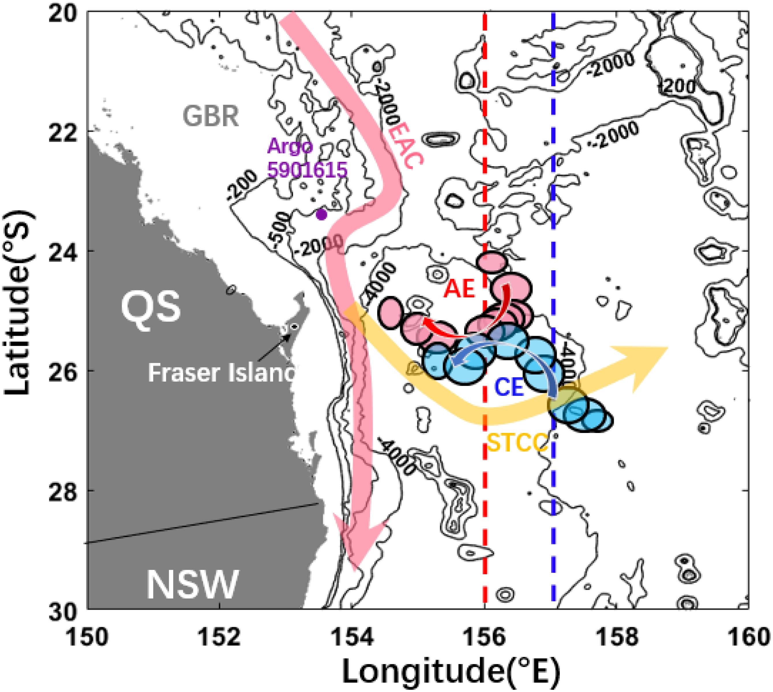
Figure 1. Geographic location of the EAC, AE and CE on a bathymetric map with depth contours (0, –200, –500, –2,000, and –4,000 m). The purple spot indicates the position of Argo float 5901615 on July 10, 2010. The southward pink arrow shows the path of the EAC. Yellow arrow indicates the South Tropical Counter Current (STCC) and Blue arrow stand for the South Caledonia Jet (SCJ). The series of pink and blue circles delineate the general movement of the cores of the AE and CE. Red and blue dashed lines indicate the sections’ location for the Hovmöller plot of the AE and CE in Figure 4. GBR stands for Great Barrier Reef, NSW represents New South Wales, and QS indicates Queensland.
The detection of eddies from the Marine Environment Monitoring Service (CMEMS) altimeter map (delayed-time gridded daily Sea Level Anomaly (SLA) with a resolution of 0.25° × 0.25°) confirmed the existence of large numbers of mesoscale eddies in the deep-basin off Fraser Island (Ribbe and Brieva, 2016). Eddy pairs are common in this region, and usually occupy most of the study areas, as observed on SLA maps. These eddy pairs locate in the study area, where the topography is complex with a substantially narrowed continental shelf at around 24°S. The deepest region, greater than 5,000 m, is to the south of 24°S in this basin, whereas the bathymetry in the north is characterized by a deep passage. Previous studies have identified the crucial role of the narrow continental shelf in regulating the EAC acceleration and separation between 28°S and 32°S (Roughan and Middleton, 2002; Cetina-Heredia et al., 2014). The sudden narrowing in the study area is also possibly a trigger for the EAC meandering, which may further influence the associated eddy fields.
To address the above unsolved questions and fill the gaps in the study area, this study aims to provide an insight of these eddies. The details of the eddies in the study area are explored by scrutinizing an eddy pair’s circulation pattern, hydrographic properties and thermal dynamics. The possible mechanisms that modulate the generation and dissipation of a representative eddy pair are also investigated. We detail the three-dimensional structure of an anticyclonic eddy (AE) and a cyclonic eddy (CE) observed off Fraser Island in the form of an eddy pair using the Bluelink Reanalysis dataset alongside satellite altimetry and Argo observations. This study will fill the gap in understanding the individual eddies’ features and how the straightforward interactions between eddies and current will induce these features. Furthermore, the heat and salt mass transports will be probed to investigate their roles to the local ocean and global ocean.
In the following contents, section “Data and Methods” introduces the data and methods used in this study. Section “Thermal and Dynamical Nature of the Eddy Pair” explores the evolution in sea surface height (SSH), relative vorticity and propagation of the detected eddy pair, together with its three-dimensional thermal and dynamic structures. In section “Potential Generation and Drivers of the Eddy-Pair,” possible contributors to the variability of the eddy pair are discussed, including the topography effect and the interactions between the EAC and the eddies. Heat and salt mass transports by the eddy pair are also investigated. Section “Conclusion” summarizes the findings in this research.
Data and Methods
The Bluelink Reanalysis (BRAN), part of the Global Ocean Data Assimilation Experiment (GODAE), was used to determine the three-dimensional structure of the eddy pair. This simulation, with assimilation of satellite-observed SSH, temperature, and in situ observations from Argo and other sources, was developed by the Commonwealth Scientific and Industrial Research Organization (CSIRO), Bureau of Meteorology and the Royal Australian Navy (Oke et al., 2009). As an ensemble optimal interpolation system, BRAN has been developed as a forecast system based on Modular Ocean Model for mesoscale ocean circulation from 1993 to 2018, and provides 51 unevenly distributed vertical layers of verified model output with a horizontal resolution of ∼10 km, which allows mesoscale ocean circulation and most features of EAC-related processes to be resolved (Mata et al., 2006). As a promising ocean hindcasting and forecasting model, BRAN has been defined as a realistic representation of mesoscale ocean circulation around Australia (Oke et al., 2008). The updated version BRAN3.5 was used in this paper. It has been validated and reanalyzed with the observational data (Oke et al., 2005, 2008, 2013b). Compared with other BRAN products such as BRAN2, it gives better dynamically consistent results for ocean variability and even extreme events (Oke et al., 2013b). Oke et al. (2013a) also validated BRAN3.5 using multi-source observations from, such as CENS-CLS09 (Rio et al., 2011) for mean sea level, the Atlas of Regional Seas from CSIRO (Ridgway and Dunn, 2003) for mixed layer depths, and AMSR-E1 (Reynolds et al., 2007) for the seasonal cycle of the modeled sea surface temperature. Further comparisons of volume transport through straits and passages, salinity, and chlorophyll content were also given. All results led to the conclusion that BRAN3.5 provides realistic predictions most of the time, with some minor errors (Oke et al., 2013a).
To ensure the reliability of BRAN3.5 in resolving the studied eddy pair, we compared the model results with observations from in situ measurements and satellite remote sensing. For example, the SLA data from the Ssalto/Duacs gridded multimission altimeter, produced and distributed by the CMEMS2 was used to evaluate the reliability of BRAN3.5 in reconstructing the evolution and transformation of the eddy pair. The daily SLA data covered the time period from 1993 to 2015 with a horizontal resolution of 0.25° × 0.25° using a 20-year dataset of mean SSH. It was further used to understand the EKE distribution in the study area.
Comparisons of sea level between BRAN3.5 and altimeter data were undertaken for the period from July 1 to September 31, 2009. An example from September 15 is presented in Figures 2A and B. Figure 2A shows the SLA from the altimeter data. Most of the sea level features presented in Figure 2A were also captured in Figure 2B, which shows horizontal maps of SSH simulated by BRAN3.5. Temperature and salinity profiled by the Argo float in the water column were compared with those extracted from BRAN3.5 for every 10 days from June to September 2010 (an example is shown in Figure 2C). Vertical distributions of temperature and salinity from BRAN3.5 showed strong agreement with those observed by the Argo profiler. Thus, it is reasonable to conclude that BRAN3.5 is sufficiently accurate for use in this study.
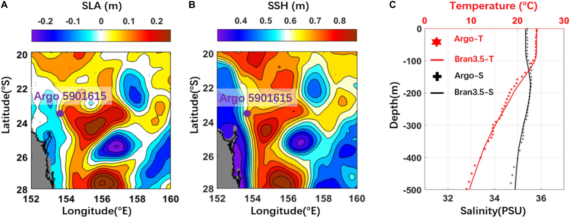
Figure 2. (A) SLA from altimeter data on September 15, 2009; (B) SSH from BRAN3.5 on September 15, 2009; (C) comparison of temperature and salinity distributions from Argo 5901615 (purple dot) and BRAN3.5 in the water column on July 10, 2010.
Thermal and Dynamical Nature of the Eddy Pair
Identification and Evolution of the Eddy Pair
Several mesoscale eddies offshore of Fraser Island were detected by BRAN3.5 from July to November 2009 (Figure 3). Among those mesoscale eddies, this research focuses on an eddy pair composed of two typical eddies (one AE and one CE). Figure 3 shows the SSH and relative vorticity in the water column, which indicates the evolution of the eddy pair in both the horizontal and vertical planes. The relative vorticity is given by , where ν is the meridional velocity and μ is the zonal velocity.
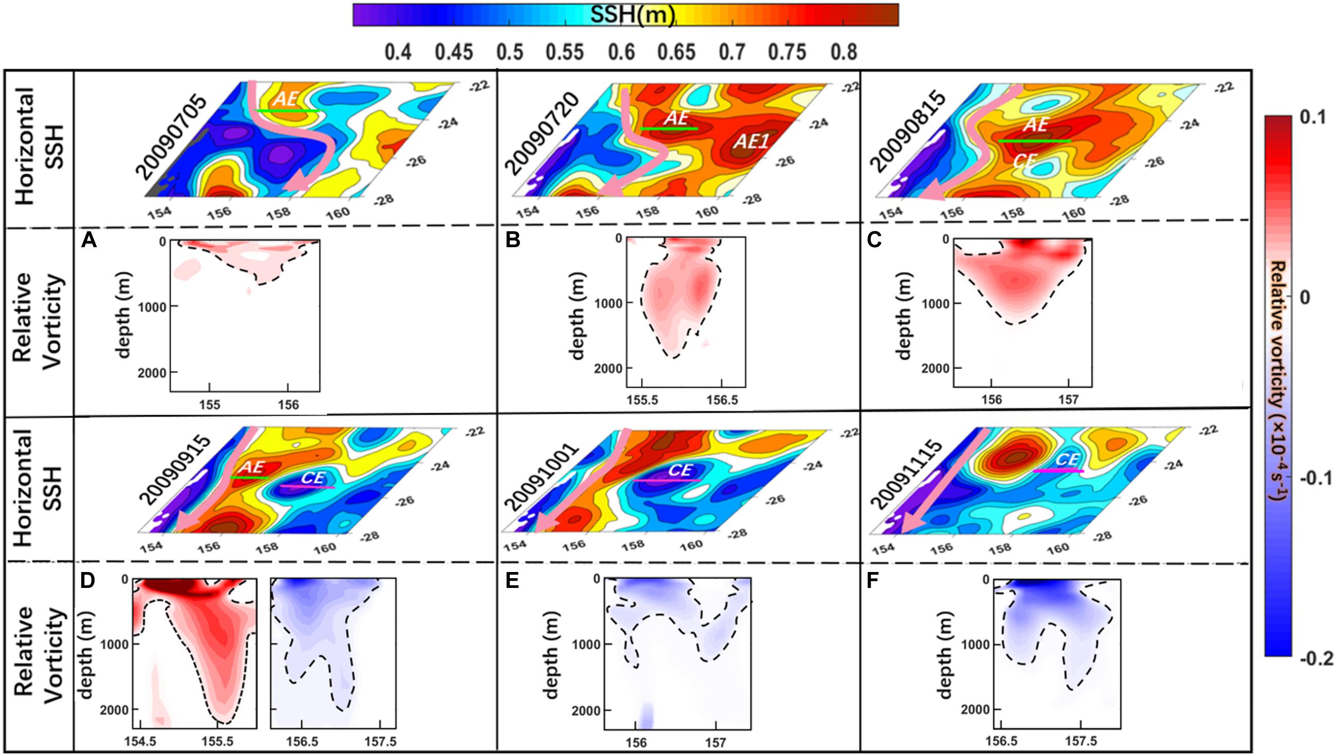
Figure 3. SSH (m) and relative vorticity obtained from BRAN3.5 from July 5 to November 15, 2009 (A–F) showing the evolution of these two eddies in both the horizontal and vertical planes. The dashed lines in the profiles of relative vorticity indicates where |ξ| = 0.02×10⁻⁴s−1 is observed. AE, anticyclonic eddy; CE, cyclonic eddy. Green and pink lines show the selected zonal sections used to determine the relative vorticity of the AE and CE, respectively. The pink southward arrows show the mainstream of the EAC.
The AE was clearly presented by the SSH on July 5 (Figure 3A), whereas the CE occurred on around August 15 (Figure 3C). Figure 3D presents a relatively mature status of both the AE and CE on September 15, 2009, when both the AE and CE showed stronger relative vorticity. The SSH during this period showed the eddy pair evolution east of 155°E between 24°S and 28°S. The AE center occurred around 154.5°E, 25°S, whereas the CE was detected at around 156.5°E, 25.8°S, 240 km away from the AE. The highest SSH contour of the AE appeared on August 15, 25 cm higher than its surrounding waters, whereas the lowest SSH in the CE occurred on September 15, 25 cm lower than the ambient values.
The CE was smaller in diameter than the AE before September 15, based on the horizontal maps of SSH. After that, the SSH of the CE showed a larger horizontal scale than the AE, as the AE started merging and became elongated while the CE was still growing. The enclosed loops of the AE and CE, side by side, were irregular ellipses. The surface SSH indicated that the AE (CE) lasted around two to three months from July (August) to September (November), 2009, respectively.
The evolution of the eddy pair in the vertical plane was analyzed by investigating profiles of the relative vorticity (ξ) in the water column beneath the CE and AE (Figure 3). On July 5, when the AE was weak and just starting to grow, the vertical profile of relative vorticity showed that AE only extended to about 800 m. As it evolved, it penetrated deeper to 2,500 m on September 15. The CE started its lifecycle on August 15 (Figure 3C). After that, the CE kept growing, and its relative vorticity was increased. The vertical profile of relative vorticity further showed that the maximum penetration depth of this CE occurred at 2,500 m on September 15 (Figure 3D), and the CE dissipated after November 15, as evidenced by the horizontal maps of SSH. The positive energy sources that support the growth and evolution of this eddy pair will be further investigated in the section “Possible Topographic Effects,” and they are possibly from the released Available Potential Energy from baroclinic instability (BCI) (Su and Ingersoll, 2016) and inverse cascading of Kinetic Energy from the smaller scale circulations/disturbances (Torres et al., 2018; Klein et al., 2019).
Figure 3 also elucidates asymmetries of the AE and CE in both the horizontal and vertical planes. For example, a strong AE was indicated by its largest SSH scope on August 15 (Figure 3C). However, the relative vorticity of the AE did not form in the water column on the same day. Instead, the positive relative vorticity associated with this AE in the water column maximized and extended much deeper on September 15, when the AE indicated by the SSH at the surface layer was greatly diminished (Figure 3D). A similar asymmetry was also observed in the CE. When its horizontal gradient of SSH dissipated toward November 15, the relative vorticity in the upper layers (shallower than 1,000 m) gradually strengthened (Figures 3E,F).
As mentioned above, the EAC in the study area is more variable and weaker than it is downstream further south, where it intensifies (Ridgway and Dunn, 2003). The AE was generated alongside the EAC, when the EAC separated from the coastline and shifts eastward. As the EAC swung back toward the coast, it shed the AE in August. Figures 3B and C indicate another AE (AE1 in Figure 3B) merged with the studied AE from July 20 to August 15. Later on, this AE propagated westward to reach and re-merge with the EAC. At the time, the CE formed, grew, and “followed” the migration of the AE to the coast. However, when the AE started merging with the EAC, it excited the instability of this strong current to stimulate a “new” AE that ceased the westward propagation of the CE, which instead moved eastward and eventually dissipated (Figures 3E,F).
Because mesoscale eddies are assumed to be propagated westward mostly by Rossby waves (Chelton et al., 2011), and given that both the AE and CE mainly shifted in the zonal direction, we selected two meridional sections at 156°E and 157°E (red and blue dashed lines in Figure 1), along which to plot Hovmöller plots (see Figure 4) and to further track the propagation of the AE and CE. In addition to the previously discussed motion in the zonal direction, this study also found that the AE propagated poleward, whereas the CE moved equatorward. Previous studies (Morrow et al., 2007; Chelton et al., 2011) presented distinct preferential behaviors for anticyclones and cyclones. These different preferential behaviors are mainly attributed to the planetary β effect and the effects of ambient currents on the propagation directions of eddies, either by meridional advection induced by the mean barotropic flow or by the effects of vertical shear on the potential vorticity gradient vector (Chelton et al., 2011). For the AE, the EAC neighboring it is a barotropic flow that may provide meridional advection, which would lead to poleward propagation. When the AE and the EAC separated in August, the poleward propagation disappeared. Interestingly, the CE seemed to be trapped by two anticyclonic vortices and to move poleward before September, then it stopped its equatorward propagation (Figure 4) when another AE appeared after October (Figures 3E,F).
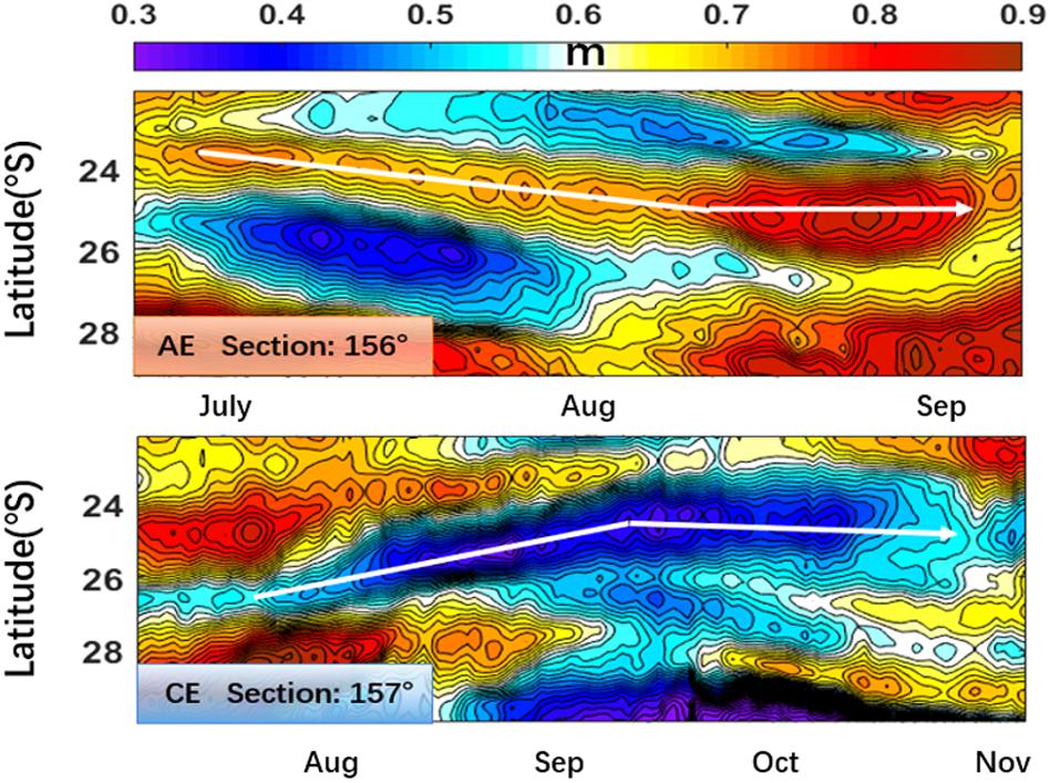
Figure 4. Hovmöller plot of the SSH time-series variation in the AE (section 156°E) and CE (section 157°E) indicating their propagation directions (white arrows).
The propagation of the AE and CE at the selected sections also indicated their lifespans. The AE was born in July and dissipated in September, whereas the CE appeared in August and disappeared in November. The AE had a shorter lifespan because of its westward propagation and merging with the EAC. This finding is also supported by the study of Chelton et al. (2011), which proposed that anticyclonic eddies alongside boundary currents tend to have shorter lifespans because of their tendency to be reabsorbed into the current.
Three-Dimensional Thermal Structures
In the previous section, we explored the general characteristics, propagation, and lifespans of the studied eddy pair by investigating the horizontal maps of SSH, relative vorticity in the water column, and Hovmöller plots of their respective meridional propagation. We detail the dynamic structure of this eddy pair in the following contents.
Inspired by our previous analyses, we scrutinized the temperature of the AE and CE on different layers to understand their thermal structures. As it is shown in Figure 3D, the AE and CE had their largest relative vorticity on September 15 (Figure 3D), so we selected this date as a case study to delineate the development stage of the eddy pair.
The temperature distribution in the AE above the mixed layer was not clearly distinguishable, possibly because of the combined impacts of the changeable heat flux, winds and ocean currents (Figure 5). We therefore selected layers from the top to bottom at depths of 260, 1,000, 1,500, and 2,300 m. The maximum temperature (19°C) in the center of the AE, ∼1°C higher than that at the edge of the AE in the water column, appeared at 260 m. An isotherm with a temperature of 16°C enclosed the CE in the same layer, and the minimum temperature in the center was 1°C lower than its adjacent waters.
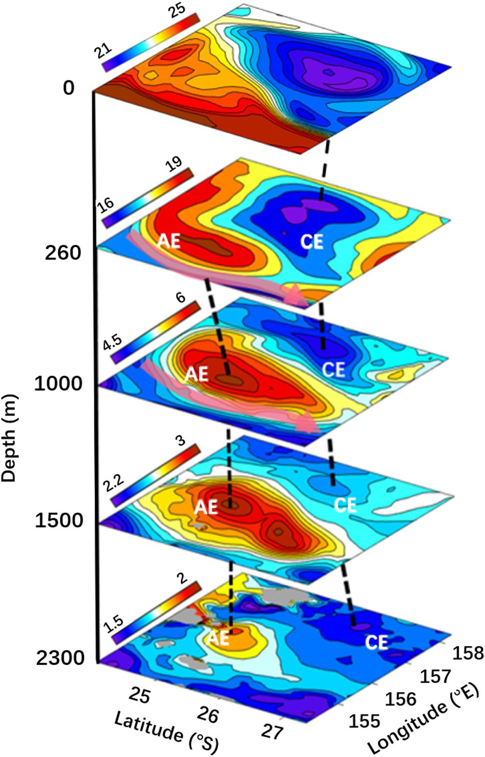
Figure 5. Temperature (°C) distributions of the AE and CE at different depths (0, 260, 1,000, 1,500, and 2,300 m) on September 15, 2009. Black dashed lines connect the cores of the AE and CE, respectively. Pink arrows indicate the location of the EAC. Note that the scale of the color bar in different layers are inconsistent to outstand the AE’s thermal feature.
At 1,000 m, the AE had the largest coverage and a clear thermal boundary on its northern side. The westward-tilting maximum temperature inside the AE above 1,000 m was toward the EAC (Figure 5). The warm core associated with the AE was 0.7°C higher, and the cold core associated with the CE 0.5°C lower, than the temperature of the surrounding water in this layer.
The temperature and its horizontal gradient in the AE gradually decreased in the greater depths below 1,000 m, and the AE had a larger volume, as indicated by both the horizontal and vertical temperature distributions. The largest diameter indicated by the thermal structure was 200 km for AE and CE. A clear temperature gradient still existed in the AE at 2,300 m, which suggested that it can penetrate to 2,300 m in the water column. In contrast, the thermal gradient in the CE decreased dramatically below 1,000 m, which indicated that its vertical penetration greatly diminished below 1,000 m. The horizontal gradient of temperature bordering the AE was also much larger than that surrounding the CE.
Temperature distributions in both the CE and AE were heterogeneous horizontally and vertically in the upper layers. For the AE, a larger horizontal temperature gradient appeared in the west where the EAC was located, and the bathymetry dramatically decreased from 4,500 to 500 m (Figure 1). This steep slope formed a barrier for the westward propagation of the AE and reshaped its western side with the effect of the EAC. However, the AE in the lower layer (2,300 m) did not show a similar pattern to that in the upper layers. At this depth, the AE was not greatly influenced by the boundary current nor by the slope. For the CE, a larger horizontal gradient in temperature mainly existed on its western side where it interacted with the AE. As mentioned above, the horizontal and vertical structures were independent based on different components. A similar situation was found in the temperature structure. The CE had a larger scope than the AE at 260 m on September 15. However, the intensity of the horizontal temperature gradient inside the CE was much smaller than that of the AE in each layer, as shown in Figure 5. The thermal structure of the AE also indicated a tilting structure of the AE because of the asymmetry discussed above (Figure 5). The AE tilted to the west in the upper layers (shallower than 1,000 m) where it interacted with the EAC. The core under 1,000 m depth was barely affected.
Dynamic Structures
The dynamic evolution of the eddy pair was briefly introduced in section “Identification and Evolution of the Eddy Pair” by examining relative vorticity. In this section, the detailed dynamic structure of the eddy pair is further explored. For consistency with the previous section, the specific dynamic structure of the eddy pair is also examined for September 15, when both the AE and CE had large relative vorticity (Figure 3D). The Okubo-Weiss method is first used to better reveal the three-dimensional dynamic structure of the eddy pair. The velocity profiles of the eddy pair are then explored to further understand the asymmetries in their dynamic structures.
The Okubo-Weiss method (Okubo, 1970; Weiss, 1991) has been widely used to determine the spatial dynamic scale of mesoscale eddies (Henson and Thomas, 2008; Isern-Fontanet et al., 2003; Hu et al., 2011; Zhang et al., 2013). Following Isern-Fontanet et al. (2003), the Okubo-Weiss parameter W, is given as follows:
Besides the relative vorticity (ξ) discussed previously, the normal (sn) and shear (ss) components of strain are defined as:
Here, μand ν are the horizontal geostrophic velocity components. To define the boundary of the eddy with the Okubo-Weiss parameter, W = −0.2σw is widely used, where σw is the standard deviation of W (Hu et al., 2011; Zhang et al., 2013). However, the selection of W also changes according to the local circumstance (Chaigneau et al., 2009, 2011), as we also adapted in this research. Once the boundary of an eddy is defined by W, an average radius, R, may be estimated by , where A is the area encircled by W.
Figure 6 shows the largest coherent scopes of the AE and CE at different layers according to the boundary contour of W. In the AE field, W contours had a quasi-circular shape at depths, compared with the temperature structures above. The CE had an obvious filament in the upper layer, which may be a result of strong shear stress on its southern side. As discussed in section “Three-Dimensional Thermal Structures,” the AE and CE penetrated downward to around 2,300 m. Both the dynamic structures from relative vorticity and the Okubo-Weiss parameter were reasonably consistent.
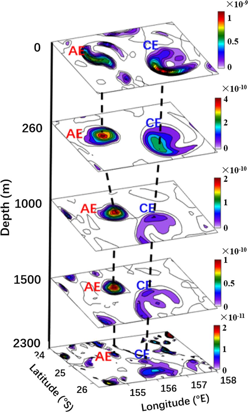
Figure 6. Spatial scales of the AE and CE indicated by their respective Okubo-Weiss parameters, which encircle the eddy and represent the largest coherent scopes at each depth. The units are s– 2.
Again, the AE had a more anomalous shape on the surface than that in the below layers. The horizontal shape of the AE did not change much as the depth increased from around 260 to 1,000 m. In comparison, the CE had a much larger horizontal scope in the upper layers. In contrast, the radius of the AE was more uniform at depth than that of the CE. From 260 to 1,500 m, the radius of the AE ranged from 62 to 50 km. Below 1,500 m toward 2,300 m, the radius of the AE decreased dramatically. The dynamic structure again indicated that the scope of the AE was much larger than that of the CE in the lower layers.
The dynamic structure in Figure 6 indicated similar information to that from the temperature structure (Figure 5). The AE tilted toward the EAC in the upper layers. As discussed above, it is possible a combined result of the planetary β effect, interaction with topography and current-eddy interaction. The AE was driven westward by the planetary β effect. However, its lower part encountered the seamounts during its western propagation, which resulted in the tilting to the coast side in the upper layers. Moreover, the relative vorticity of the AE was smaller than the local Coriolis parameter, hence the AE is easily entrained by the EAC. All these factors could contribute to the titling of the AE. The vertical structure of the CE was much more independent, and the CE had a larger horizontal scale than the AE in the upper layer, but that scale decreased rapidly with increased depth. The AE tended to have a more coherent and uniform structure above 1,500 m. Based on the dynamic structures of the eddy pair defined above, the water mass volumes trapped by the AE and CE were 2.73 × 10¹³ and 5.92 × 10¹² m3, respectively. The volume of the AE thus was around an order of magnitude larger than that of the CE.
To better understand the asymmetric structure of the eddy pair shown in the thermal and dynamic structures, the vertical profiles of horizontal velocity associated with the AE and CE were analyzed using BRAN3.5. Velocity is a very important feature of eddies that can be used to investigate the vertical profile of the eddy pair. Figure 7A shows the maxima of the horizontal velocity of a cross-section (155°E) through the center of the AE. The vertical profile of the CE was through the center of the CE at the cross-section along 157°E (shown by a black line) on the same day. The velocity of the eddy pair in the upper ocean (above 500 m) reached a maximum value of 0.5 m/s. The velocity decreased to 0.1 m/s as depth decreased to ∼2,000 m for the AE and CE.
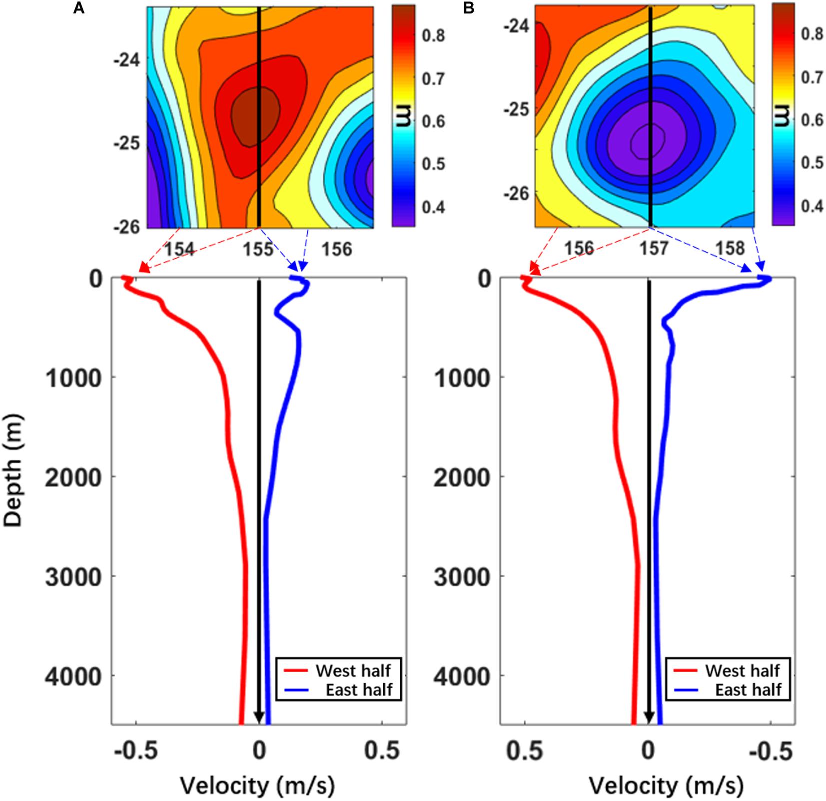
Figure 7. (A) The maxima of horizontal velocities encircling the AE in the west half (red line) and east half (blue line) of 155°E from 23.2°S to 25.5°S on September 15; (B) vertical distribution of the maxima of the horizontal velocity encircling the CE in the west half (red line) and east half (blue line) of 157°E from 26.5°S to 23.8°S on September 15. Black lines in (A) and (B) incise the center sections of the AE and CE. Positive values indicate southward velocity while negative values indicate northward velocity. Note that the x-axis has a reversal sign in (B).
Interestingly, the maximum velocity on the western side of the AE almost doubled that on its eastern side at the sub-surface (below 300 m), consistent with the asymmetry found above. The asymmetry on the western side of the AE (stronger SSH gradient) was possibly due to the intensification caused by the EAC. In the CE, the western side presented a higher velocity than the eastern side. As found in the temperature distribution, this was possibly because of the interaction between the AE and the CE. The rotation directions of the AE and CE were opposite, but the rotation direction for both AE and CE were the same where they interacted. The larger velocity on the western side of the CE may have been strengthened by the AE.
Potential Generation and Drivers of the Eddy-Pair
The above results detailed the three-dimensional structures and evolution of the eddy pair based on examination of their hydrographic properties, relative vorticity, and the Okubo-Weiss parameters. This section explores possible factors contributing to the eddy-pair evolution, including the topography and energy transfer (baroclinic/barotropic instability). As eddies are important contributors to regulating heat and salt balance in the ocean, the heat and salt mass transports by the eddy pair are also estimated.
Ocean eddies are usually affected by one or more of topographic steering, and barotropic instability (BTI) or BCI in the mean flows (Shore et al., 2008; Zhan et al., 2014). As a next step, we explore these possible factors in the eddy field. Topographic steering, which has a significant impact on boundary flow, has little effect in deep water, as is the case in most of the study area. However, the deep bathymetry can provide space for the generation of large eddies. The BCI and BTI of the mean flow are usually considered as major sources of eddy formation at the boundary of the global ocean circulation gyre (Qiu et al., 2009; Zhang et al., 2013; Bulczak et al., 2015). These possible contributors to the eddy pair are explored below.
Possible Topographic Effects
To quantify the variation in the eddy activity, we determined the EKE throughout the region from the velocities calculated from the SLA data provided by CMEMS. These values were annually averaged over the study domain based on daily SLA data. In this study, we calculated the EKE for the year 2009. The formula used in this study is:
Here, h′ is the SSH anomaly in units of meter, g is the gravitational constant (9.8 m/s2), and f is the Coriolis parameter determined based on the latitude.
The annually averaged EKE distribution over the entire study area in 2009 is shown in Figure 8. The high EKE in the study area was comparable to the ambient seas which have been identified as high EKE regions. Qiu and Chen (2004) calculated the averaged (from 1992 to 2002) EKE of several bands near and in this study area as previously introduced. In their estimation, the averaged EKE in the area inside 5°S– 15°S and 150°E–170°W was 242 cm2/s2, while the EKE over the EAC region inside 25°S–40°S and 150°E–167°E was 452 cm2/s2. The averaged EKE (201 cm2/s2) in our study area was comparable with that in the former area and half of that in the later area in Qiu and Chen (2004). Thus, it is important and necessary to investigate the eddy-related processes in the seas to the east of Fraser Island, due to its high EKE.
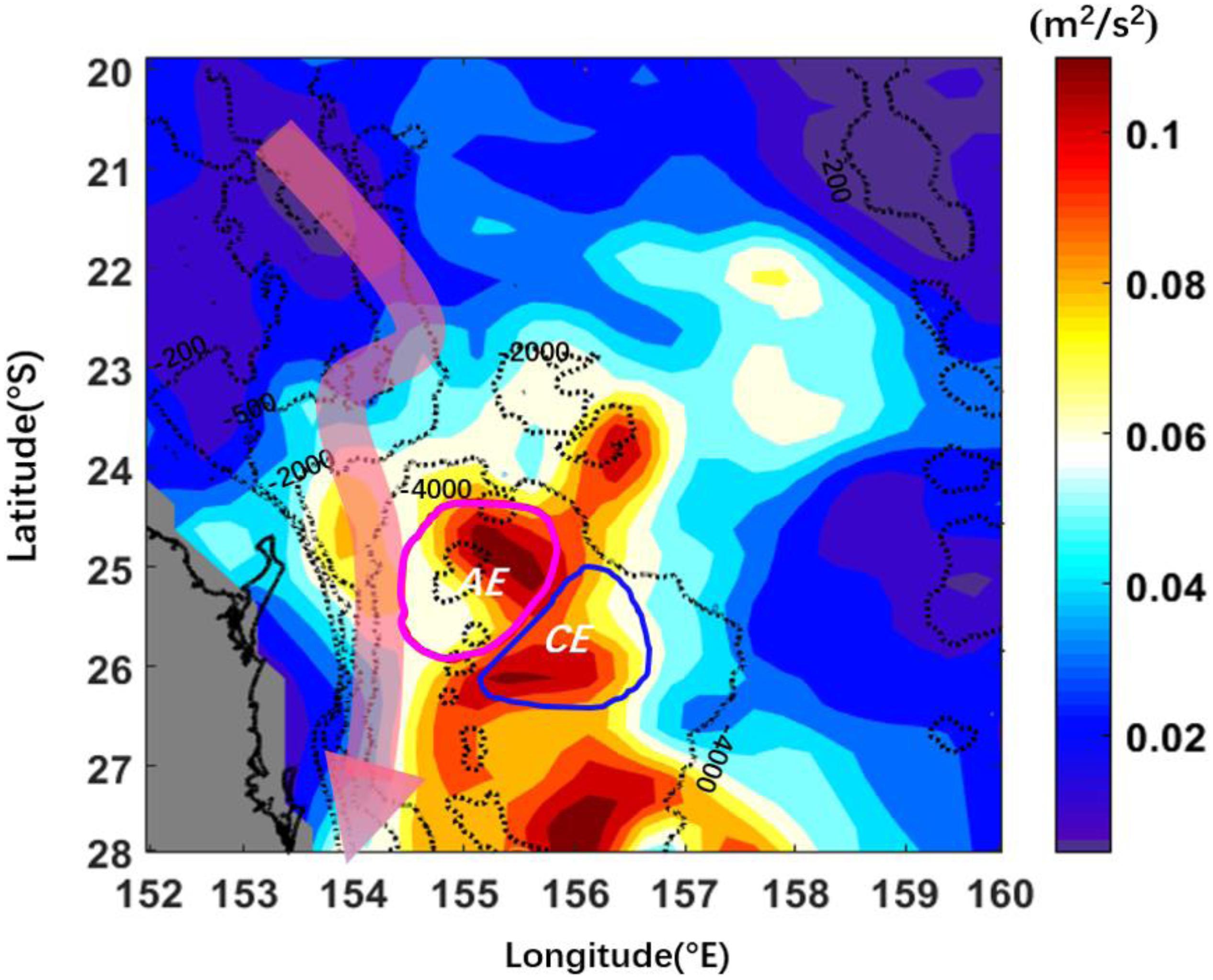
Figure 8. Annually averaged EKE distribution over the study area in 2009, showing the high EKE in the deep middle basin. Black dotted lines are the bathymetry contours. Pink arrow indicates the EAC location. Pink (blue) quasi-circles are the AE (CE) locations.
Another surprising finding was that the high EKE in the middle basin (24°–28°S and 155°–158°E) was not on the eastern boundary of the study area, to which many eddies were expected to be transported westward from the eastern high eddy-activity field by Rossby waves. This interesting phenomenon may indicate that the high EKE was not a result of eddy propagation from the eastern eddy-activity field, and that locally generated eddies existed and may even have accounted for the majority of the total number of eddies. The averaged EKE in the middle basin was twice that in the surrounding water body, which could be attributed to the deep bathymetry that favored the generation of strong eddies, as deep bathymetry provides space for the eddy generation. The AE and CE were generated in the boundary area (e.g., 2,000 to 4,000 m) of the deep basin (Figure 1). As they evolved and propagated to the Tasman basin, they continued to grow and then dissipated near the continental slope and the seamounts (Figure 1), respectively. Thereby, bottom friction induced by topography was important to allow energy cascading to a smaller scale and energy dissipation. The topography in the study area may favor the generation of these mesoscale eddies according to the EKE distribution. The complex topography is also possibly responsible for the energy cascading and dissipation of these eddies in the study area.
In addition, the EAC variability is an important factor in eddy generation, as previously summarized. The instability induced by the local topography is possibly responsible for the EAC meanders (Bowen et al., 2005), and the narrowing of the continental shelf topography is linked to the EAC’s acceleration and separation (Oke and Middleton, 2001; Roughan and Middleton, 2002). Cetina-Heredia et al. (2014) further concluded that the narrow points in the continental shelf favored the EAC separation. Thus, the sudden narrowing of the continental shelf in the study area is also a possible trigger of the variations in the EAC. Furthermore, the EKE greatly increased in the south of the narrow point in our study area (around 24°S), which may also manifest the significance of the narrowing point to the EAC variation. However, a more precise conclusion of the topographic effects is not able to be resolved in this study and will be explored in the future.
Diagnosis of Energy Transition
Energy in the ocean takes different forms including the mean kinetic energy (MKE), EKE, mean available potential energy (MPE), and available eddy potential energy (EPE) (Xie et al., 2007; Von Storch et al., 2012; Zhan et al., 2014). The exact MPE and EPE are not easily calculated, but the energy transfer between the eddy energy components can be determined by analyzing the eddy energy budget (Von Storch et al., 2012; Zhan et al., 2014). Positive BCI values indicate that MPE is converted to EPE in this process. Negative BCI values denote that EPE is converted to MPE. Conversely, positive BTI values indicate energy transfer from MKE to EKE, and negative BTI values show that EKE is converted to MKE. The BCI has been found in previous studies to be a principal source of energy for ocean eddies (Wang and Ikeda, 1997; Stammer, 1998; Zhang et al., 2013). However, the AE interacted with the EAC, which is a strong geostrophic flow and releases high BTI. It is interesting to attempt to diagnose which were the major sources in this case. We used simulations from BRAN 3.5 to distinguish between the contributions of these factors to the eddy field throughout July to October 2009.
The contributions from the BCI/BTI (Baroclinic/Barotropic conversion term) in the study area in 2009 were calculated by the following equations (Oey, 2008; Zhang et al., 2013):
Here, u′ and v′ are the corresponding velocity anomalies referring to the annually averaged zonal and meridional velocities in 2009. To calculate the terms above and be consistent with the previous part of this study, we used the data from BRAN3.5. The variable N in the BCI equation denotes the Brunt-Väisälä frequency, given by , where the variable ρ0 (1027 kg m–3) is the reference density of sea water. is the annually averaged density in 2009, and ρ′ denotes the density anomaly referring to . In this study, we calculated the vertically integrated BCI and BTI in the upper 800 m of the ocean, where majority of the energy in the eddy pair is expected to have been stored, according to their relative vorticity distribution (Figure 3D).
In July and September, the area-averaged BCI in the AE presented large positive values (Figure 9A). These positive values indicated that the BCI released potential energy to the AE in these periods. In contrast, the mean BTI in the AE was much smaller. Both the BCI and BTI were positive contributors to the CE in the growing stage, and therefore were possible major energy sources for the CE (Figure 9B). It should also be noted that during the growing stage, AE may be the main supplier for the potential and kinetic energy as it is closely interacted with the CE, and the merging of AE1 toward the studied AE shown in Figure 3B further strengthened the BCI from July to August. In October, the BTI in the CE was negative, which indicated that a large amount of kinetic energy was drained from the CE. As discussed in section “Identification and Evolution of the Eddy Pair,” this occurred after the AE disappeared in late September (Figure 9B). The contributions of BCI and BTI to the AE were much larger than those to the CE. This finding can explain the differences in the scales of these two eddies: more energy was input to the AE, which resulted in the larger hydrographic scale of the AE; similarly, less energy input led to a smaller hydrographic scale for the CE.
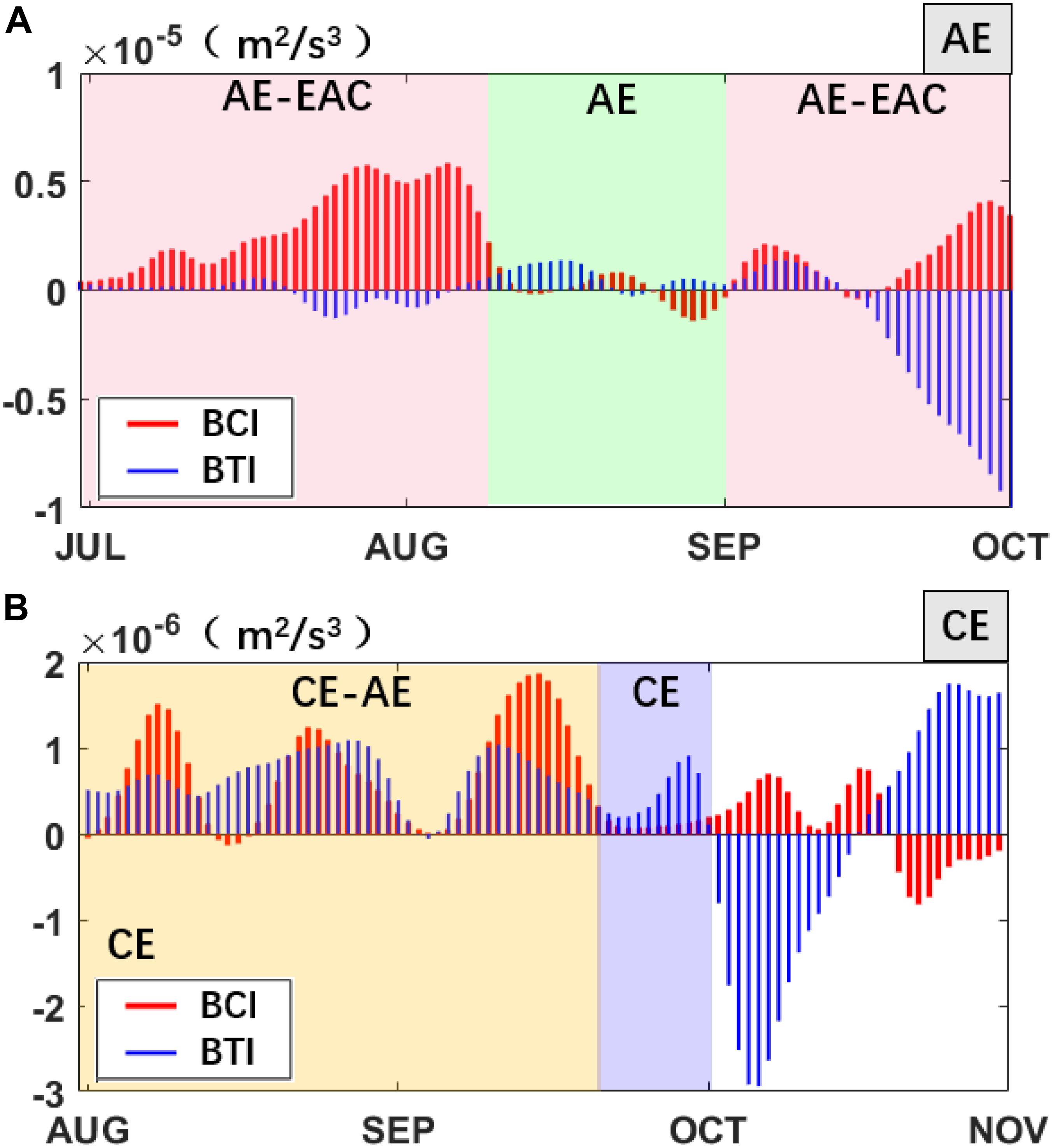
Figure 9. Variation of the daily area-averaged BCI and BTI in the (A) AE and (B) CE. Units are m3/s3. Pink background in (A) indicates the period when the AE interacted with the EAC; green background indicates the separation period for the AE and the EAC. Yellow background in (B) indicates the periods when the CE interacted with the AE, whereas blue background represents the period after the AE disappeared.
As previously noted, the BCI was a main contributor to the AE in July and September, which was the period when the AE interacted with the EAC. Besides, the largest BCI input lasted from mid-July to mid-August, when the AE1 was merging with the AE as mentioned in section “Identification and Evolution of the Eddy Pair.” To investigate the combined role that the EAC and the AE1 played in generating and interacting with the AE, we analyzed monthly variation of BCI/BTI.
The first row in Figure 10 shows the geographical relationship between the EAC and the AE. In July, when the AE was growing, the EAC flow-field interfered with the AE. As the EAC shifted back to the coastal area (section “Identification and Evolution of the Eddy Pair”), the EAC and the AE separated. This phenomenon was also clearly identified from the velocity profile for August (Figure 10). The AE propagated westward until it finally reached the EAC and started to merge with it. Correspondingly, the vertical BCI profiles of the AE were positive on the western side in July, negative in August, and positive again in September because of the above-mentioned attachment and detachment from the EAC. Furthermore, the AE had a large positive BCI on its eastern side in August, which is possibly a result of the merging event with AE1. BTI showed a similar pattern but with a much smaller magnitude. All of these findings verified that the BCI and BTI for the AE were mainly from the EAC and the merging event with AE1.
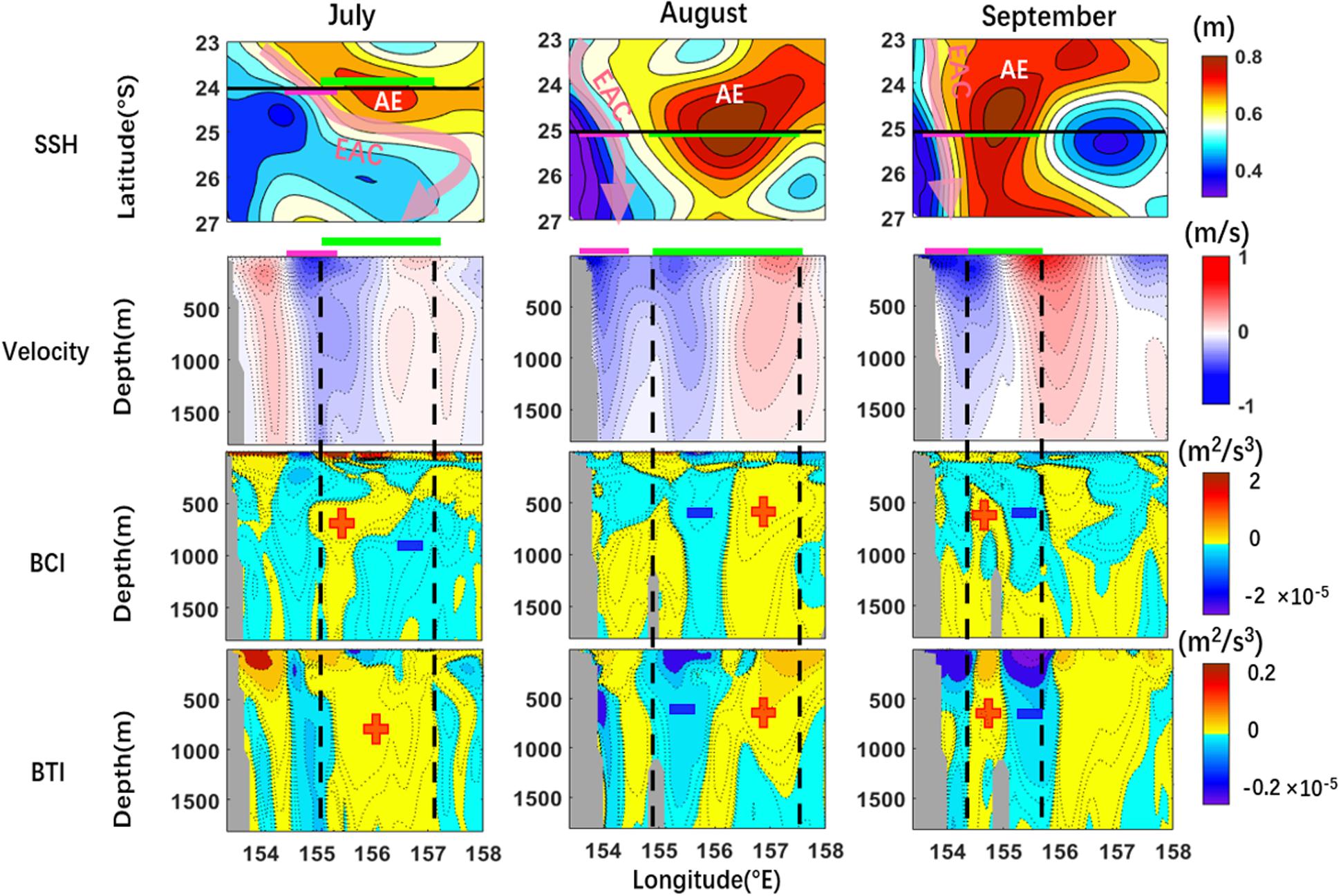
Figure 10. First row: monthly averaged SSH for the AE. Pink lines are the sections across the EAC, and green lines are the sections across the AE. Second row: vertical profile of meridional velocity along the section across the center of the EAC and the AE (corresponding pink/green lines). The northward current was indicated by warm color in these plots. Third row: vertical profile of monthly averaged BCI. Fourth row: vertical profile of monthly averaged BTI. Different color-scales in the third and fourth rows are used to better illustrate the characteristics of EAC and AE.
Previous analyses on the eddy pair further confirm the energy transfer during the interactions among eddies and the interactions between the AE and the EAC. The BCI in the AE greatly diminished from early August (Figure 9A) when it separated from the EAC and its poleward propagation ceased (Figure 4A). Likewise, the BCI in the CE was positive (Figure 9B) before the CE ceased its equatorward propagation and detached from the AE (Figure 4B). The above energy transfer analyses are also coincident with the explanations of the structures of the AE and the CE. The AE and CE’s tilting structures were results of the eddy-current and eddy-eddy interactions: the AE had a tilting structure on the EAC side and the CE tilted to the AE while they interacted. The asymmetry of the velocity on the western and eastern sides of the AE and CE can be revealed by the energy transfer analyses. The AE had a higher speed on its western side, where it gained energy from the EAC. Similarly, the speed of the CE on the western side was higher than that on its eastern side as it gained energy from the AE.
Zonal Heat and Salt Mass Transports by the Eddy Pair
Mesoscale eddies are regarded as important contributors to the heat balance at a global scale (Wunsch, 1999; Dong et al., 2014), especially in the western boundary current areas (Roemmich and Gilson, 2001). Several estimations of heat and salt mass transports based on the Eulerian framework are widely used, and mostly related to the covariation of temperature and velocity anomalies under different assumptions (Stammer, 1998; Qiu and Chen, 2004; Meijers et al., 2007; Volkov et al., 2008). Dong et al. (2014) calculated the global heat and salt mass transports by mesoscale eddies in a Lagrangian framework. The particular dynamic structures of eddies determine the uplift or depression of the pycnocline profiles that lead to T/S anomalies inside the eddies. The induced T/S anomalies (with respect to the background pycnocline) embedded in the eddy field tend to travel with the eddies when the inside waters are trapped. Thus, the heat and salt of an eddy can be transported by its movement. Because we have focused on an individual westward-propagating eddy pair, the Lagrangian method was employed as it gives better estimations of heat and salt mass transports.
According to Dong et al. (2014), zonal heat and salt mass transports can be calculated as shown below. For a single eddy with a radius R and horizontal movement velocity (the eddy movement between two time steps, which is one day in this study), the vertical T/S anomaly profiles are and ( and are calculated by referring to the annually averaged zonal velocity, temperature and salinity in 2009, respectively):
The units of Eqs 6 and 7 are W and kg/s, respectively. The averaged density () in the upper layer and heat capacity (Cp) are 1.025 × 10³ kg/m3 and 4.20 × 10³ J/(kg°C), respectively. Eddies have been categorized into three shapes (bowl, lens, and cone) (Dong et al., 2014). The AE and CE were lens- and bowl-shaped, as shown in previous 3D hydrographic and hydrodynamic structures, with the coefficients S is used as 1 and 0.5, respectively.
Thus, the zonal heat transported by the AE and CE in this study was calculated to be 2.31 × 10¹⁴ W and 5.51 × 10¹³ W, and the zonal salt mass transported 1.65 × 10⁹and 1.26 × 10⁸ kg/s, respectively. According to Dong et al. (2014), the time-averaged zonal heat and salt mass transports by eddies around 25°S in the Pacific Ocean were approximately 2 × 10¹⁴ W and 1 × 10⁹ kg/s, respectively, which are of the same order of magnitude as the amounts for the AE. In contrast, the zonal heat transported by the CE was much smaller than that estimated in Dong et al. (2014). The previously discussed structure and energy input differences can account for the small amount of heat and salt mass transports by the CE. Thus, referring to the aforementioned amounts of heat and salt mass transported by eddies zonally integrated along 25°S in the Pacific Ocean (Dong et al., 2014), both the heat and salt mass transports and horizontal/vertical scales indicate that the studied eddies in the Southern Coral Sea are not negligible with respect to the local ocean conditions.
Conclusion
This study has helped identifying mesoscale eddies offshore from Fraser Island, which have rarely been explored in previous studies. Past studies examined eddies off the northeast coast of Australia formed by the EAC separation (O’Kane et al., 2011; Suthers et al., 2011; Roughan et al., 2017; Oke et al., 2019; Malan et al., 2020), mostly between 30°S and 34°S, giving rise to the Tasman Front (Suthers et al., 2011; Cetina-Heredia et al., 2014). Little attention has been devoted to details of eddies north of the separation points-especially the eddy pair phenomena, which occur frequently. This work focuses on mesoscale eddies in the deep basin and offshore from Fraser Island. It addresses the gap in understanding the detailed temporal and spatial scales of these eddies. An eddy pair (AE and CE) lasting from July to November 2009 in this area was selected to understand the detailed hydrographic features of these eddies. BRAN3.5 was employed to provide confirmation and further insight into the details of this eddy pair, including their propagation, thermal structures, dynamic structures, energy transfer, and heat and salt mass transports.
The maxima of the horizontal scale of the AE and CE is about 200 km, about half the size of the largest eddies (∼400 km) in the EAC separation points. However, the scale was still comparable to the average scales (∼100 km) of the global eddies at similar latitudes (Chelton et al., 2011). The thermal and dynamic structures gave a comprehensive depiction of the eddy pair, their possible mutual interaction and the interaction with the EAC. The structures also provided further details for heat and salt calculation. The large amounts of zonal heat and salt mass transports by the eddy pair, especially those carried by the AE, were not negligible. The heat and salt mass transports by this AE were of the same order of magnitude as the zonal averaged eddies. Thus, we determined that both the horizontal/vertical structures and the heat and salt mass transports indicated that this eddy pair in the study area is non-negligible with respect to the local ocean conditions. As there was a large number of eddies (over 50 per year) in this region as detected by Everett et al. (2012), the total heat and salt mass transports could be considerable. However, the capacity of heat and salt mass transports by individual eddies varies in a wide range, more details about the total heat and salt mass transports will be explored in the future study. The high EKE (∼201 cm2/s2) possibly indicated high eddy activities in the study area which further emphasized the significance of the study eddy field.
Asymmetries in horizontal/vertical structures were found in both the AE and CE. The most energetic profiles (based on relative vorticity) occurred later than the largest horizontal scope for both the AE and CE. When the horizontal scope was merging or dissipating, this eddy pair indicated by relative vorticity in the water column still existed. It would be interesting to further investigate the continuous effects of the eddies after their surface appearance had disappeared. For the AE, it tilted into the side of the EAC in the upper layers. The details of the interaction between the AE and the EAC were explored based on energy analysis. The CE had a weaker thermal/dynamic structure, which was explained through the energy diagnosis.
Energy analysis was carried out to determine the energy contributions of the BCI and BTI to the eddy pair. The BCI contributed energy to the AE in the generation stage when the AE was close to the EAC and merged with the AE1, indicating that the BCI generating the AE was mainly from the EAC and a merging event. As the EAC changed its path and moved toward the coast, this strong current drained energy from the AE, rather than injecting energy into it. After the AE propagated westward and reached the EAC in the coastal area, the EAC recharged energy into it. Because the CE was far from the EAC, it was unlikely to directly receive energy from this strong western boundary current. However, the BCI and BTI provided to the CE may have been derived from the AE and surrounding circulations. The dynamical genesis of eddy pairs and their detailed temporal-spatial evolution will be further investigated in our future studies.
It should be noted that although this research detailed the spatial and temporal evolution of an eddy pair to the east of EAC, mesoscale processes with a horizontal extent less than 50 km are difficult to investigate due to limitations in the observations and numerical simulations. The studied mesoscale process here is more like a coherent vortex in Tarshish et al. (2018). It should also be noticed that the sub-mesoscale symmetric instability possibly exists universally and characterizes a large proportion of the ocean (Yu et al., 2019b), which also plays an important role in modulating the upper oceans stratification (Yu et al., 2019a,b), for example, the sub-mesoscale processes could be five times larger than the mesoscale processes in modulating the vertical heat transport (Su et al., 2018). However, due to the limited resolution of the used simulation, the sub-mesoscale processes cannot be well resolved. The underlying dynamics associated with the sub-mesoscale and fine structures of the eddy pair will be further investigated in our near-future studies by using ultra-high resolution (e.g., 1 km) numerical simulations.
Data Availability Statement
The datasets presented in this study can be found in online repositories. The names of the repository/repositories and accession number(s) can be found below: http://dap.nci.org.au/thredds/remoteCatalogService?catalog=http://dapds00.nci.org.au/thredds/catalog/gb6/BRAN/BRAN3p5/catalog.xml.
Author Contributions
ZBL conducted the analyses and wrote the manuscript. XW and JH as well as FPA read through the manuscript and provided their revisions. ZQL is the corresponding author that designed the structure and sciences of this research. All authors contributed to the article and approved the submitted version.
Conflict of Interest
FPA was employed by Wikiletters.org.
The remaining authors declare that the research was conducted in the absence of any commercial or financial relationships that could be construed as a potential conflict of interest.
The reviewer NM declared a shared affiliation with several of the authors ZBL and XW to the handling editor at the time of review.
Acknowledgments
This work was supported by the National Natural Science Foundation of China (41906016 and 41776027), and the Science, Technology and Innovation Commission of Shenzhen Municipality (JCYJ20190809144411368), Key Special Project for Introduced Talents Team of Southern Marine Science and Engineering Guangdong Laboratory (Guangzhou) (GML2019ZD0210). FPA acknowledges support from the CNPq fund at IO-USP (152424/2019-9). This is publication number 84 of the Sino-Australian Research Centre for Coastal Management. Data used in this project was supported by the Sino-Australian Research Centre for Coastal Management. The results of the simulations from BRAN3.5 can be found at http://dap.nci.org.au/thredds/remoteCatalogService?catalog=http://dapds00.nci.org.au/thredds/catalog/gb6/BRAN/BRAN3p5/catalog.xml.
Footnotes
References
Boland, F. M., and Church, J. A. (1981). The east Australian current 1978. Deep Sea Res. Part A Oceanogr. Res. Pap. 28, 937–957. doi: 10.1016/0198-0149(81)90011-X
Bowen, M. M., Wilkin, J. L., and Emery, B. (2005). Variability and forcing of the East Australian current. J. Geophys. Res. Oceans 110:C03019.
Bulczak, A. I., Bacon, S., Naveira Garabato, A. C., Ridout, A., Sonnewald, M. J., and Laxon, S. W. (2015). Seasonal variability of sea surface height in the coastal waters and deep basins of the Nordic Seas. Geophys. Res. Lett. 42, 113–120. doi: 10.1002/2014gl061796
Bull, C., Kiss, A. E., Jourdain, N. C., England, M. H., and van Sebille, E. (2017). Wind forced variability in eddy formation, eddy shedding, and the separation of the East Australian Current. J. Geophys. Res. Oceans 122, 9980–9998. doi: 10.1002/2017jc013311
Bull, C. Y., Kiss, A. E., van Sebille, E., Jourdain, N. C., and England, M. H. (2018). The role of the New Zealand plateau in the Tasman Sea circulation and separation of the East Australian current. J. Geophys. Res. Oceans 123, 1457–1470. doi: 10.1002/2017JC013412
Cetina-Heredia, P., Roughan, M., Van Sebille, E., and Coleman, M. A. (2014). Long-term trends in the East Australian current separation latitude and eddy driven transport. J. Geophys. Res. Oceans 119, 4351–4366. doi: 10.1002/2014JC010071
Chaigneau, A., Eldin, G., and Dewitte, B. (2009). Eddy activity in the four major upwelling systems from satellite altimetry (1992-2007). Prog. Oceanogr. 83, 117–123. doi: 10.1016/j.pocean.2009.07.012
Chaigneau, A., Texier, M. L., Eldin, G., Grados, C., and Pizarro, O. (2011). Vertical structure of mesoscale eddies in the eastern South Pacific Ocean: a composite analysis from altimetry and Argo profiling floats. J. Geophys. Res. 116:C11025. doi: 10.1029/2011JC007134
Chelton, D. B., Schlax, M. G., and Samelson, R. M. (2011). Global observations of nonlinear mesoscale eddies. Prog. Oceanogr. 91, 167–216. doi: 10.1016/j.pocean.2011.01.002
Dong, C., McWilliams, J., Liu, Y., and Chen, D. (2014). Global heat and salt transports by eddy movement. Nat. Commun. 5:3294. doi: 10.1038/ncomms4294
Everett, J. D., Baird, M. E., Oke, P. R., and Suthers, I. M. (2012). An avenue of eddies: quantifying the biophysical properties of mesoscale eddies in the Tasman Sea. Geophys. Res. Lett. 39:16608. doi: 10.1029/2012GL053091
Glenn, S. M., and Ebbesmeyer, C. C. (1994). The structure and propagation of a Gulf Stream frontal eddy along the North Carolina shelf break. J. Geophys. Res. Oceans 99, 5029–5046. doi: 10.1029/93JC02786
Henson, S. A., and Thomas, A. C. (2008). A census of oceanic anticyclonic eddies in the Gulf of Alaska. Deep Sea Res. Part I Oceanogr. Res. Pap. 55, 163–176. doi: 10.1016/j.dsr.2007.11.005
Hu, J., Gan, J., Sun, Z., Zhu, J., and Dai, M. (2011). Observed three dimensional structure of a cold eddy in the southwestern South China Sea. J. Geophys. Res. Oceans 116:C05016. doi: 10.1029/2010jc006810
Isern-Fontanet, J., García-Ladona, E., and Font, J. (2003). Identification of marine eddies from altimetric maps. J. Atmos. Ocean Technol. 20, 772–778. doi: 10.1175/1520-0426(2003)20<772:iomefa>2.0.co;2
Ismail, M. F. A., Ribbe, J., Karstensen, J., Lemckert, C., Lee, S., and Gustafson, J. (2017). The Fraser Gyre: a cyclonic eddy off the coast of eastern Australia. Estuary Coast. Shelf Sci. 192, 72–85. doi: 10.1016/j.ecss.2017.04.031
Kawabe, M. (1995). Variations of current path, velocity, and volume transport of the Kuroshio in relation with the large meander. J. Phys. Oceanogr. 25, 3103–3117. doi: 10.1175/1520-0485(1995)025<3103:vocpva>2.0.co;2
Klein, P., Lapeyre, G., Siegelman, L., Qiu, B., Fu, L. L., Torres, H., et al. (2019). Ocean-scale interactions from space. Earth Space Sci. 6, 795–817. doi: 10.1029/2018ea000492
Malan, N., Archer, M., Roughan, M., Cetina-heredia, P., Hemming, M., Rocha, C., et al. (2020). Eddy-driven cross-shelf transport in the east australian current separation zone. J. Geophys. Res. Oceans 125, 1–15. doi: 10.1029/2019JC015613
Marchesiello, P., and Middleton, J. H. (2000). Modeling the East Australian current in the western Tasman Sea. J. Phys. Oceanogr. 30, 2956–2971. doi: 10.1175/1520-0485(2001)031<2956:mteaci>2.0.co;2
Mata, M. M., Tomczak, M., Wijffels, S. E., and Church, J. A. (2000). East Australian current volume transports at 30 degrees: estimates from the World ocean circulation experiment hydrographic sections PR11/P6 and the PCM3 current meter array. J. Geophys. Res. Oceans 105, 28509–28526. doi: 10.1029/1999jc000121
Mata, M. M., Wijffels, S. E., Church, J. A., and Tomczak, M. (2006). Eddy shedding and energy conversions in the East Australian current. J. Geophys. Res. Oceans 111:C09034. doi: 10.1029/2006JC003592
Meijers, A. J., Bindoff, N. L., and Roberts, J. L. (2007). On the total, mean, and eddy heat and freshwater transports in the southern hemisphere of a 1/8° ×1/8° global ocean model. J. Phys. Oceanogr. 37, 277–295. doi: 10.1175/JPO3012.1
Morrow, R., Birol, F., Griffin, D., and Sudre, J. (2007). Divergent pathways of cyclonic and anti-cyclonic ocean eddies. Geophys. Res. Lett. 31:L24311.
Oey, L. Y. (2008). Loop current and deep eddies. J. Phys. Oceanogr. 38, 1426–1449. doi: 10.1175/2007JPO3818.1
O’Kane, T. J., Oke, P. R., and Sandery, P. A. (2011). Predicting the East Australian Current. Ocean Model. 38, 251–266. doi: 10.1016/j.ocemod.2011.04.003
Oke, P. R., Brassington, G. B., Griffin, D. A., and Schiller, A. (2008). The Bluelink ocean data assimilation system (BODAS). Ocean Model. 21, 46–70. doi: 10.1016/j.ocemod.2007.11.002
Oke, P. R., Brassington, G. B., Griffin, D. A., and Schiller, A. (2009). Data assimilation in the Australian Bluelink system. Mercator Ocean Quarterly Newsletter 34, 35–44.
Oke, P. R., and Griffin, D. A. (2011). The cold-core eddy and strong upwelling off the coast of New South Wales in early 2007. Deep Sea Res. Part II Top. Stud. Oceanogr. 58, 574–591. doi: 10.1016/j.dsr2.2010.06.006
Oke, P. R., Griffin, D. A., Schiller, A., Matear, R. J., Fiedler, R., Mansbridge, J. V., et al. (2013a). Evaluation of a near-global eddy-resolving ocean model. Geosci. Model. Dev. 6, 591–615. doi: 10.5194/gmdd-5-4305-2012
Oke, P. R., Sakov, P., Cahill, M. L., Dunn, J. R., Fiedler, R., Griffin, D. A., et al. (2013b). Towards a dynamically balanced eddy-resolving ocean reanalysis: BRAN3. Ocean Model. 67, 52–70. doi: 10.1016/j.ocemod.2013.03.008
Oke, P. R., and Middleton, J. H. (2001). Nutrient enrichment off Port stephens: the role of theEast Australian current. Continent. Shelf Res. 21, 587–606. doi: 10.1016/S0278-4343(00)00127-8
Oke, P. R., Roughan, M., Cetina-Heredia, P., Pilo, G. S., Ridgway, K. R., Rykova, T., et al. (2019). Revisiting the circulation of the East Australian current: its path, separation, and eddy field. Prog. Oceanogr. 176, 102139.1–102139.20.
Oke, P. R., Schiller, A., Griffin, D. A., and Brassington, G. B. (2005). Ensemble data assimilation for an eddy-resolving ocean model of the Australian region. Q. J. R. Meteorol. Soc. 131, 3301–3312. doi: 10.1256/qj.05.95
Okubo, A. (1970). Horizontal dispersion of floatable particles in the vicinity of velocity singularities such as convergences. Deep Sea Res. Oceanogr. Abstracts 17, 445–454. doi: 10.1016/0011-7471(70)90059-8
Qiu, B., and Chen, S. (2004). Seasonal modulations in the eddy field of the South Pacific Ocean. J. Phys. Oceanogr. 34, 1515–1527. doi: 10.1175/1520-0485(2004)034<1515:smitef>2.0.co;2
Qiu, B., Chen, S., and Kessler, W. S. (2009). Source of the 70-day mesoscale eddy variability in the Coral Sea and the North Fiji Basin. J. Phys. Oceanogr. 39, 404–420. doi: 10.1175/2008JPO3988.1
Reynolds, R. W., Smith, T. M., Liu, C., Chelton, D. B., Casey, K. S., and Schlax, M. G. (2007). Daily high-resolution-blended analyses for sea surface temperature. J. Clim. 20, 5473–5496. doi: 10.1175/2007JCLI1824.1
Ribbe, J., and Brieva, D. (2016). A western boundary current eddy characterisation study. Estuar. Coast. Shelf Sci. 183, 203–212. doi: 10.1016/j.ecss.2016.10.036
Ridgway, K. R. (2007). Long term trend and decadal variability of the southward penetration of the East Australian current. Geophys. Res. Lett. 34:L13613.
Ridgway, K. R., and Dunn, J. R. (2003). Mesoscale structure of the mean East Australian current system and its relationship with topography. Prog. Oceanogr. 56, 189–222. doi: 10.1016/S0079-6611(03)00004-1
Ridgway, K. R., and Godfrey, J. S. (1994). Mass and heat budgets in the East Australian current: a direct approach. J. Geophys. Res. Oceans 99, 3231–3248. doi: 10.1029/93JC02255
Ridgway, K. R., and Godfrey, J. S. (1997). Seasonal cycle of the East Australian current. J. Geophys. Res. Oceans 102, 22921–22936. doi: 10.1029/97JC00227
Rio, M. H., Guinehut, S., and Larnicol, G. (2011). New CNES-CLS09 global mean dynamic topography computed from the combination of GRACE data, altimetry, and in situ measurements. J. Geophys. Res. Oceans 116:C07018. doi: 10.1029/2010JC006505
Roemmich, D., and Gilson, J. (2001). Eddy transport of heat and thermocline waters in the North Pacific: a key to interannual/decadal climate variability? J. Phys. Oceanogr. 31, 675–687. doi: 10.1175/1520-0485(2001)031<0675:etohat>2.0.co;2
Roughan, M., Keating, S. R., Schaeffer, A., Cetina-Heredia, P., Rocha, C., Griffin, D., et al. (2017). A tale of two eddies: the biophysical characteristics of two contrasting cyclonic eddies in the East Australia current system. J. Geophys. Res. Oceans 122, 2494–2518. doi: 10.1002/2016JC012241
Roughan, M., and Middleton, J. H. (2002). A comparison of observed upwelling mechanisms off the east coast of Australia. Continent. Shelf Res. 22, 2551–2572. doi: 10.1016/S0278-4343(02)00101-2
Schaeffer, A., and Roughan, M. (2015). Influence of a western boundary current on shelf dynamics and upwelling from repeat glider deployments. Geophys. Res. Lett. 42, 121–128. doi: 10.1002/2014GL062260
Shevenell, A. E., Kennett, J. P., and Lea, D. W. (2004). Middle Miocene southern ocean cooling and Antarctic cryosphere expansion. Science 305, 1766–1770. doi: 10.1126/science.1100061
Shore, J., Stacey, M. W., and Wright, D. G. (2008). Sources of eddy energy simulated by a model of the northeast Pacific Ocean. J. Phys. Oceanogr. 38, 2283–2293. doi: 10.1175/2008JPO3800.1
Stammer, D. (1998). On eddy characteristics, eddy transports, and mean flow properties. J. Phys. Oceanogr. 28, 727–739. doi: 10.1175/1520-0485(1998)028<0727:oeceta>2.0.co;2
Su, Z., and Ingersoll, A. P. (2016). On the minimum potential energy state and the eddy size-constrained APE density. J. Phys. Oceanogr. 46, 2663–2674. doi: 10.1175/JPO-D-16-0074.1
Su, Z., Wang, J., Klein, P., Thompson, A. F., and Menemenlis, D. (2018). Ocean submesoscales as a key component of the global heat budget. Nat. Commun. 9:775. doi: 10.1038/s41467-018-02983-w
Suthers, I. M., Young, J. W., Baird, M. E., Roughan, M., Everett, J. D., Brassington, G. B., et al. (2011). The strengthening East Australian Current, its eddies and biological effects—an introduction and overview. Deep Sea Res. Part 2 Top. Stud. Oceanogr. 58, 538–546. doi: 10.1016/j.dsr2.2010.09.029
Tarshish, N., Abernathey, R., Zhang, C., Dufour, C. O., Frenger, I., and Griffies, S. M. (2018). Identifying Lagrangian coherent vortices in a mesoscale ocean model. Ocean Model. 130, 15–28. doi: 10.1016/j.ocemod.2018.07.001
Tilburg, C. E., Hurlburt, H. E., O’Brien, J. J., and Shriver, J. F. (2001). The dynamics of the East Australian current system: the Tasman Front, the East Auckland current, and the East Cape current. J. Phys. Oceanogr. 31, 2917–2943. doi: 10.1175/1520-0485(2001)031<2917:tdotea>2.0.co;2
Torres, H. S., Klein, P., Menemenlis, D., Qiu, B., Su, Z., Wang, J., et al. (2018). Partitioning ocean motions into balanced motions and internal gravity waves: a modeling study in anticipation of future space missions. J. Geophys. Res. Oceans 123, 8084–8105. doi: 10.1029/2018JC014438
Volkov, D. L., Lee, T., and Fu, L.-L. (2008). Eddy-induced meridional heat transport in the ocean. Geophys. Res. Lett. 35:L20601. doi: 10.1029/2008GL035490
Von Storch, J., Eden, C., Fast, I., Haak, H., Hernández-Deckers, D., Maier-Reimer, E., et al. (2012). An estimate of the Lorenz energy cycle for the world ocean based on the STORM/NCEP simulation. J. Phys. Oceanogr. 42, 2185–2205. doi: 10.1175/jpo-d-12-079.1
Wang, J., and Ikeda, M. (1997). Diagnosing ocean unstable baroclinic waves and meanders using quasi-geostrophic equations and Q-Vector method. J. Phys. Oceanogr. 27, 1158–1172. doi: 10.1175/1520-0485(1997)027<1158:doubwa>2.0.co;2
Weiss, J. (1991). The dynamics of enstrophy transfer in two-dimensional hydrodynamics. Phys. D Nonlinear Phenomena 48, 273–294. doi: 10.1016/0167-2789(91)90088-q
Wunsch, C. (1999). The interpretation of short climate records, with comments on the North Atlantic and Southern Oscillations. Bull. Am. Meteorol. Soc. 80, 245–255. doi: 10.1175/1520-0477(1999)080<0245:tioscr>2.0.co;2
Xie, L., Liu, X., and Pietrafesa, L. J. (2007). Effect of bathymetric curvature on Gulf Stream instability in the vicinity of the Charleston Bump. J. Phys. Oceanogr. 37, 452–475. doi: 10.1175/jpo2995.1
Yu, X., Naveira Garabato, A. C., Martin, A. P., Buckingham, C. E., Brannigan, L., and Su, Z. (2019a). An annual cycle of submesoscale vertical flow and restratification in the upper ocean. J. Phys. Oceanogr. 49, 1439–1461. doi: 10.1175/jpo-d-18-0253.1
Yu, X., Naveira Garabato, A. C., Martin, A. P., Evans, D. G., and Su, Z. (2019b). Wind-forced symmetric instability at a transient mid-ocean front. Geophys. Res. Lett. 46, 11281–11291. doi: 10.1029/2019gl084309
Zhan, P., Subramanian, A. C., Yao, F., and Hoteit, I. (2014). Eddies in the Red Sea: a statistical and dynamical study. J. Geophys. Res. Oceans 119, 3909–3925. doi: 10.1002/2013jc009563
Keywords: East Australian Current, eddy pair, eddy transmission, eddy evolution, eddy-circulation interactions
Citation: Li ZB, Wang XH, Hu JY, Andutta FP and Liu Z (2020) A Study on an Anticyclonic-Cyclonic Eddy Pair Off Fraser Island, Australia. Front. Mar. Sci. 7:594358. doi: 10.3389/fmars.2020.594358
Received: 13 August 2020; Accepted: 12 November 2020;
Published: 08 December 2020.
Edited by:
Arnaud Laurent, Dalhousie University, CanadaReviewed by:
Ahmad Fehmi Dilmahamod, Dalhousie University, CanadaNeil Christopher Malan, University of New South Wales, Australia
Copyright © 2020 Li, Wang, Hu, Andutta and Liu. This is an open-access article distributed under the terms of the Creative Commons Attribution License (CC BY). The use, distribution or reproduction in other forums is permitted, provided the original author(s) and the copyright owner(s) are credited and that the original publication in this journal is cited, in accordance with accepted academic practice. No use, distribution or reproduction is permitted which does not comply with these terms.
*Correspondence: Zhiqiang Liu, liuzq@sustech.edu.cn