Numerical Simulation of Inline Forces on a Bottom-Mounted Circular Cylinder Under the Action of a Specific Freak Wave

Freak waves pose a great threat to the tension-leg platforms (TLPs) and monopile foundations of offshore wind turbines (OWTs), which necessitates comprehensive investigations on the characteristics of freak waves and the wave actions on those offshore renewable energy structures with circular cylinder. The recorded freak wave series “New Year Wave” (NYW) was numerically simulated using the Computational Fluid Dynamics methods. The compensation measure was adopted to effectively improve simulation accuracy. Under the action of the NYW, the inline forces and secondary load cycle (SLC) on a vertical-mounted cylinder, as the classic form for the TLPs and foundation of OWTs, were fully addressed. The simulation results were compared with the empirical formulations and experimental data to reveal the differences and the possible causes. The development of SLC was found to be closely related to the downstream vortex and return flow, which induces the reduction of the wall pressure and thus the inline force. The maximum inline forces vary with the cylinder position relative to the wave peak, and the simulation results reveal that the linear inline forces calculated by Morison formulation may be less than 65% of the total wave forces.

Introduction

With the utilization of the renewable marine energy and resources, the offshore structures, including the tension-leg platforms (TLPs) and offshore wind turbines (OWTs) have rapidly developed over the past few decades. Cylindrical structures, e.g., the support structures for TLPs and monopile foundations of the OWTs, are the most common structural forms in ocean engineering, which are easily threatened by extreme freak waves. Freak waves may occur on a calm sea and reach very high amplitude. Klinting and Sand (1987) defined freak waves with the following criteria: (1) H_i > 2H_s; (2) H_i > H_i–1, H_i > H_i+1; (3) η_c > 0.65H_i, where H_i and H_s represent the maximum wave height and the significant wave height, H_i–1 and H_i+1 are the immediate wave height before and after H_i, and η_c is the crest height of the maximum wave. Given the difficulty in fully satisfying the above conditions in a real sea environment, Kharif and Pelinovsky (2003) proposed regarding H_i > 2H_s as the criterion of freak waves. One such example, the “New Year Wave” (NYW, with a maximum wave height of 25 m, and the significant wave height is 10.6 m) in the North Sea, recorded at the Draupner platform on January 1st, 1995 (Haver, 2003), is a well-known representative freak wave. Freak wave is believed to be one major culprit to destruct marine structures and ships (Kharif and Pelinovsky, 2003; Bertotti and Cavaleri, 2008; Kharif et al., 2009), and would pose great threats to the wind turbines, offshore platforms, etc. Therefore, the actions of the freak wave on the marine structures should be discreetly studied to guarantee a safe design.

The freak wave has attracted wide attentions, most of previous studies are limited to moderate waves. For the simulation of the freak wave, it is usually treated as a focused wave, and a large amount of experimental and numerical investigations on the generation of the focused waves have been conducted. Tromans et al. (1991) proposed the NewWave theory, by which the target wave can be effectively generated in the experimental wave tank. Chaplin (1996) proposed the phase convergence method to experimentally generate the focused wave. Based on the wave spectrum energy distribution, Kriebel and Alsina (2000) proposed a method to simulate focused waves and its effectiveness was verified in the wave tank. For the numerical simulation methods, Ning et al. (2008) adopted the quadratic higher order boundary element model to numerically generate the focused waves, and the efficiency of this method was verified. Pakozdi et al. (2016) simulated freak waves by using Star-CCM+, in which the fluid was considered to be inviscid and incompressible. Ghadirian et al. (2016) applied the OceanWave3D potential flow wave model and a coupled OceanWave3D-OpenFOAM solver to simulate two- and three-dimensional focused waves, and the results agree well with those of the experiments.

Many methods were proposed to calculate the wave forces (Morison et al., 1950; Rainey, 1995), and some attempts were also made to predict the higher-order wave forces based on the third-order perturbation theories (Faltinsen et al., 1995; Molin, 1995). However, there were limitations to apply those theories to calculate the higher-harmonic wave forces (Rainey, 2007; Paulsen et al., 2014). Experimental and numerical explorations have been extensively performed to reveal the higher-harmonic non-linear characteristics of wave forces induced by the extreme waves. Chaplin et al. (1997) and Bredmose and Jacobsen (2010) experimentally studied the inline forces on the cylinder structures under the action of the freak wave, and found that the maximum wave forces are larger than the results calculated by Morison formulation. Chen et al. (2018) experimentally studied the non-linear harmonic components of hydrodynamic forces on a fixed cylinder and found the linear forces are only about 60% of the total forces for some cases. Deng et al. (2016) experimentally investigated the freak wave forces acting on a vertical cylinder, and the inline force is found to be closely related to the wave steepness. Liu et al. (2019) numerically studied the freak wave loads on a small diameter cylinder using OpenFOAM. A high slamming force is observed under the spilling breaking waves induced by the hitting of the local flow with high horizontal velocity on the structure. Ning et al. (2017) found the fully non-linear potential flow theory could well predict the maximum pressure on the structure under the action of focused wave. Kim et al. (2012) found that the inline force can be doubled when the wave elevation increased by 25%. Tang et al. (2020) numerically studied the effects of breaking wave loads on a 10-MW large-scale monopile offshore wind turbine, and found the breaking wave created larger inline forces than the traveling wave, and the Morison formulation would underestimate the wave load. Besides, as mentioned by Bachynski and Moan (2014), none of the aforementioned theoretical approaches could capture the secondary load cycle (SLC) that was observed in experimental and numerical studies, and Grue et al. (1993) believed that SLC makes a crucial contribution to higher-harmonic component of inline force, which may cause the ringing vibrations of the marine structures.

To the authors’ knowledge, the previous simulations for the specific freak wave “NYW” were not accurate enough, which may cause errors in the simulation of wave forces and its higher-harmonic components. In this study, the specific freak wave series, “NYW,” is numerically simulated and further modified. The non-linear inline forces acting on a bottom-mounted vertical cylinder (widely used for the support structures for TLPs and monopile foundations of the OWTs) and the characteristics of the SLC are analyzed. The remainder of the paper is organized as follows. The numerical methodology is introduced in section 2. In section 3, the two-dimensional (2-D) numerical models are used to simulate the “NYW,” and the simulation accuracy is verified. In section 4, the three-dimensional (3-D) numerical simulation of the actions of the “NYW” on a vertical cylinder is presented. The non-linear wave forces and the SLC are comprehensively investigated. In section 5, the influences of wave front steepness (kA) on the non-linear wave force, and the effects of the flow fields on the SLC magnitude are investigated. Finally, the conclusions are given in section 6.

Numerical Methodology

Governing Equations of Fluid

The time-filtered Navier-Stokes equations in the Eulerian frame were applied to describe the incompressible, viscous fluid flow. The continuity and momentum conservation equations can be presented as:

$${\displaystyle \frac{\partial {\overline{u}}_i}{\partial x_i}}=0(\mathrm{1a})$$

$${\displaystyle \frac{\partial {\overline{u}}_i}{\partial t}}+{\displaystyle \frac{\partial {\overline{u}}_i{\overline{u}}_j}{\partial x_j}}=-{\displaystyle \frac{1}{\mathrm{\rho }}}{\displaystyle \frac{\partial \overline{p}}{\partial x_i}}+{\displaystyle \frac{\partial }{\partial x_j}}\left(\mathrm{\nu }{\displaystyle \frac{\partial {\overline{u}}_i}{\partial x_j}}-\overline{u_i^{\prime }{u}_j^{\prime }}\right)+f_i(\mathrm{1b})$$

where t is the time, and x_i and x_j (i,j = 1, 2, and 3) and ith and jth Cartesian coordinates, ${\overline{u}}_i$ and $u_i^{\prime }$denote the time-averaged and fluctuating flow velocity components, respectively, $\overline{p}$denotes the time-averaged pressure, ρ and υ are the fluid density and kinematic viscosity. f_i represents the volume force. The pressure-implicit with splitting of operators (PISO) algorithm was used for the solution of pressure-velocity coupling. The second order upwind scheme was used for the momentum term. The least-squares cell-based scheme was used for gradient terms.

Free Surface Tracking

The volume of fluid (VOF) (Hirt and Nichols, 1981) scheme was adopted to simulate the two-phase flow and the Geo-reconstruct scheme enables to capture the free surface, and the volume ratio relation between two phases and transport equation can be presented as:

$${\displaystyle \sum _{q=1}^2}{\mathrm{\alpha }}_q=1(q=1,2)(\mathrm{2a})$$

$${\displaystyle \frac{\partial {\mathrm{\alpha }}_q}{\partial t}}+{\overline{u}}_i\cdot \nabla {\mathrm{\alpha }}_q=0(\mathrm{2b})$$

where α_q is the volume fraction, representing the volume fraction coefficient of the fluid. When the cell is full of the water, the value of the volume fraction is 1, and when the cell is empty of water, the value is 0. Besides, the parameter is between 0 and 1 when the cell interface between the two phases cuts the cell, therefore the volume fraction can be evaluated as:

$$\mathrm{\alpha }(x,t)=\{\begin{array}{c}\hfill \mathrm{\alpha }=1\mathit{\hspace{1em}\hspace{1em}\hspace{1em} }Water\hfill \\ \hfill (0,1)\mathit{\hspace{1em}\hspace{1em}\hspace{1em} }interface\hfill \\ \hfill \mathrm{\alpha }=0\mathit{\hspace{1em}\hspace{1em}\hspace{1em} }air\hfill \end{array}\begin{array}{}\end{array}(3)$$

Wave Generation

The dynamic grid methods were applied to simulate the piston-type wavemaker, and the transfer function (Tr) between wave height (H) and wavemaker stroke (S) can be written as:

$$Tr=\frac{H}{S}=\frac{4{\sinh }^2(kd)}{2kd+\sinh (2kd)}(4)$$

where k and d are the wave number and still water depth, respectively.

For the wave absorbing methods, a source term was introduced into the momentum equation to avoid wave reflection. The damping term was added to the momentum equation to construct the following wave elimination equation:

$${\displaystyle \frac{\partial u}{\partial t}}+u{\displaystyle \frac{\partial u}{\partial x}}+w{\displaystyle \frac{\partial u}{\partial z}}=-{\displaystyle \frac{1}{\mathrm{\rho }}}{\displaystyle \frac{\partial p}{\partial x}}+w\left({\displaystyle \frac{{\partial }^{2}u}{\partial x^2}}+{\displaystyle \frac{{\partial }^{2}u}{\partial z^2}}\right)-\mathrm{\mu }(x)u(\mathrm{5a})$$

$${\displaystyle \frac{\partial v}{\partial t}}+u{\displaystyle \frac{\partial u}{\partial x}}+w{\displaystyle \frac{\partial u}{\partial z}}=-{\displaystyle \frac{1}{\mathrm{\rho }}}{\displaystyle \frac{\partial p}{\partial z}}+w\left({\displaystyle \frac{{\partial }^{2}v}{\partial x^2}}+{\displaystyle \frac{{\partial }^{2}v}{\partial z^2}}\right)-\mathrm{\mu }(w)w(\mathrm{5b})$$

where u and w denote the velocity components in the x and z directions, respectively. μ(x) and μ(z) are the corresponding attenuation coefficients, which can be respectively calculated as:

$$\mathrm{\mu }(x)=a_x{\displaystyle \frac{x-x_1}{x_2-x_1}}(\mathrm{6a})$$

$$\mathrm{\mu }(z)=a_z{\displaystyle \frac{x-x_1}{x_2-x_1}}(\mathrm{6b})$$

where the empirical coefficients a_x and a_z in the x and z direction were set as 0.5 and 4, respectively, x₁ and x₂ are the boundaries of the wave absorbing zone.

The “NYW” was recorded at a sampling frequency of 2.133 Hz in North Sea in 1995, and the wave series are shown in Figure 1A. Considering the wave crest occurred at 264 s, the wave series from 120 to 500 s were selected as the target to save the calculation resources, the number of the total data is 812. In addition, the target wave series were simulated at a scale of 1:100 based on the Froude similarity criterion. Therefore, the sampling frequency of the scaled wave series is 21.333 Hz and the frequency intervals Δf = 0.0263 Hz.

FIGURE 1

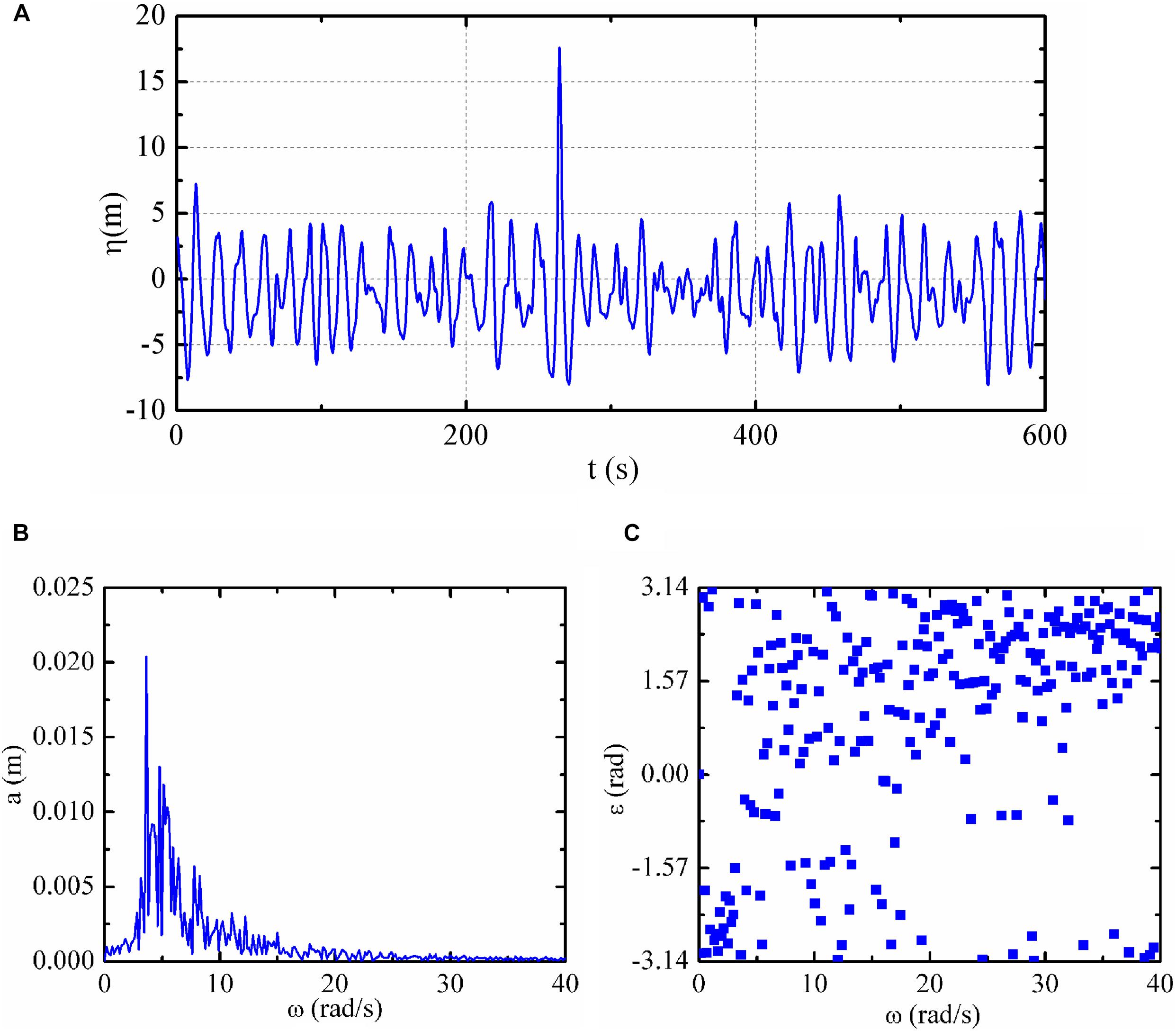
Figure 1. “NYW” recorded in the North Sea. (A) Wave elevations, (B) amplitude, and (C) initial phase.

The superposition of the simple harmonics (Longuet-Higgins, 1974) was carried out to generate the focused wave at specified location and time, the wave surface elevations (η) can be calculated as:

$$\mathrm{\eta }(x,t)=\sum _{i=1}^N{a}_i\cos (k_{i}x-{\mathrm{\omega }}_{i}t-{\mathrm{\epsilon }}_i)(7)$$

where k_i, a_i, and ε_i are the component wave numbers, amplitudes and the initial phases, respectively. For the scaled wave series, and the FFT decomposition was performed to obtain a_i and ε_i, which are shown in Figures 1B,C, respectively. Besides, a_i with higher frequency (ω ≥ 30 rad/s) components were almost negligible and only 182 wave components were incorporated for the mathematical formulations of the target wave series.

Numerical Simulation of “NYW”

To improve the simulation efficiency, the 2-D numerical model without the cylinder was firstly built up to simulate the “NYW.” The numerical wave tank (Figure 2) is 15 m long, with a 2.5 m length of wave absorbing zone. The still water depth is 0.9 m. The wave surface elevations at 11 positions (arranged with the uniform interval of 0.1 m) were monitored.

FIGURE 2

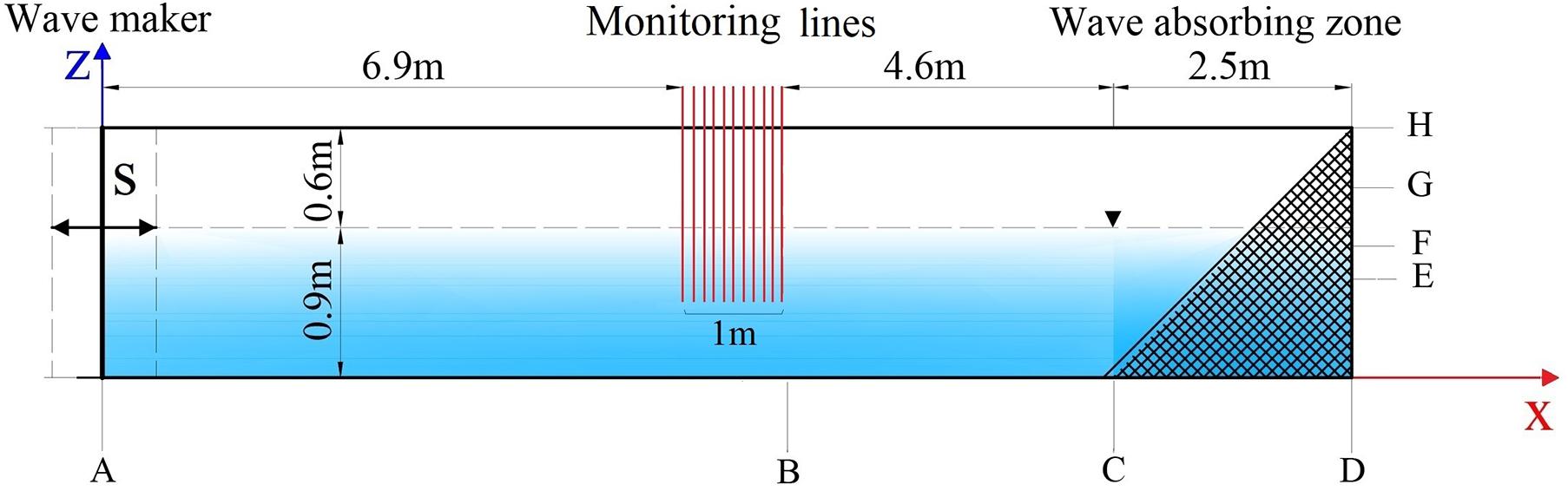
Figure 2. General arrangement sketch of the 2-D wave tank.

A mesh convergence study was carried out for the numerical simulation of the “NYW.” The mesh arrangements for the 2-D numerical models are list in Table 1.

TABLE 1

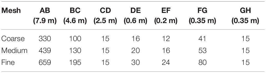
Table 1. Summary of grid parameters in the 2-D models.

The target wave series were numerically reproduced at x = 7.3 m and the horizontal velocity of the wavemaker can be presented as:

$$U_1(t)=\sum _{i=1}^N\frac{2a_i{\mathrm{\omega }}_i}{T{r}_i}\cos \left[k_i(x-7.3)-{\mathrm{\omega }}_{i}t-{\mathrm{\epsilon }}_i\right](8)$$

The calculating time step (Δt) is preliminarily set as 0.001 s. The simulated waves with stable wave from the Coarse, Medium, and Fine mesh cases, and the target wave surface elevation (η) are shown in Figure 3A, where η_c is the crest height, and the stable simulated results were selected to quantify the error. Because the control signal of the wavemaker was based on the linear wave theory which takes no consideration of non-linearity effects and the wave-wave non-linear interaction. Even with the fine mesh model, the errors for the initially calculated H and η_c are 14.4 and 22.9%, respectively, and the standard deviation for theΔη₁(t)is 0.018, whereΔη₁(t) represents the differences between η₀(t) and η₁(t). The time-step interval convergence analyses were also conducted, 0.002, 0.001, and 0.0005 s, respectively. The results of wave elevations with three time-steps were shown in Figure 3B. It is clearly found that the errors between the simulation results and the target values cannot be further reduced by improving the grid quality and decreasing the time-step.

FIGURE 3

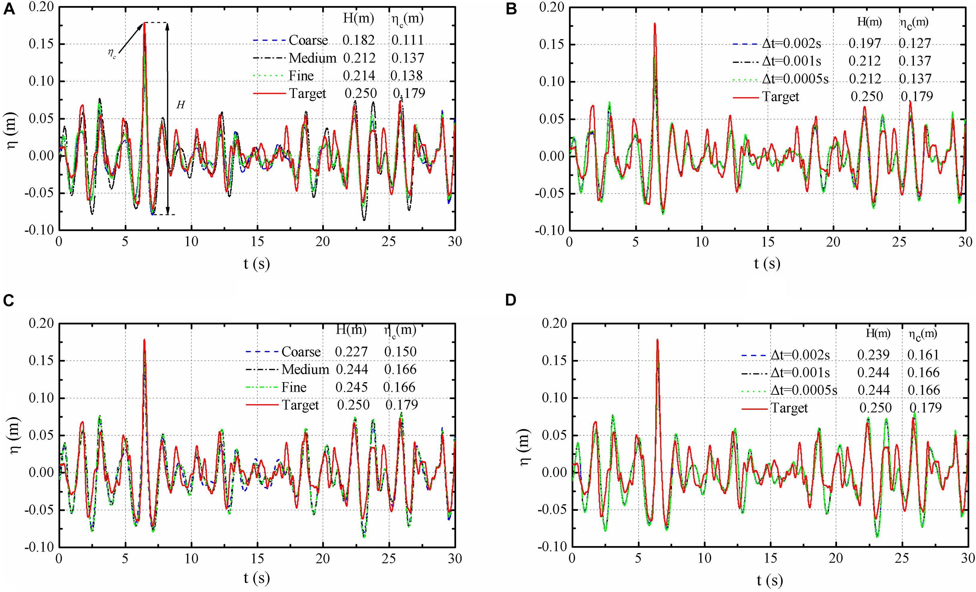
Figure 3. Grid and time-step refinement results. (A) Non-modified grid convergence, (B) non-modified time-step convergence, (C) modified grid convergence, and (D) modified time-step convergence.

The wavemaker control signal required to be modified to eliminate the deviations between the initial simulated wave elevations η₁(t) and the target data η₀(t). The modification for the horizontal velocity of the wavemaker can be presented as:

$$U_2\left(t\right)=\left(1+c\right)U_1\left(t\right)-U_1^{\prime }\left(t\right)(9)$$

where U₁(t) and $U_1^{\prime }(t)$ represent the wavemaker horizontal velocities. c is the modification coefficient, which is not only affected by the numerically simulated H and η_c, but also the simulated mild random waves. The modification quality criteria could set as: the errors for the simulated H and η_c need to be less than 4.8 and 7.6%, respectively, which approximate a third of the errors for the initial simulation. Besides, the standard deviation forΔη₂(t) [whereΔη₂(t) = η₂(t)−η₀(t)] should be less than 0.020, which is approximately 1.1 times larger than the standard deviation forΔη₁(t). The optimal c can be obtained after several attempts.

It’s worth noting that the optimal values of c may be different in those three mesh cases. Therefore, the Fine mesh model was selected as the standard case to obtain the optimal c. And the same value was used in the other mesh cases to simulate the wave series. After several attempts, 0.18 was selected as the optimal value and the newly-calculated results for the three mesh cases are shown in Figure 3C. Both H and η_c are much closer to the target values than those without using the modification technique. The errors for the newly- calculated H and η_c are 2.4 and 7.3%, respectively. In order to further evaluate the effectiveness of the modification method, kth (k = 1, 2, 3, and 4) order statistics of Δη₁(t) and Δη₂(t)were calculated, which denote the mean value, standard deviation, skewness and kurtosis, respectively. The first four orders statistic ofΔη₁(t)are 0.0032, 0.018, 0.157, and 3.598, respectively. And the first four orders statistic of Δη₂(t) are 0.0024, 0.019, 0058, and 3.239, respectively. The results by using the Medium and Fine meshes are fairly close. In addition, it is apparent that (Figures 3B,D) time-step convergence is reached for Δt = 0.001 s. It is clear that the modification method can improve the simulation accuracies of H and η_c without sacrificing the simulation quality of the mild random wave series. So, the Medium mesh and Δt = 0.001 s were adopted in consideration of both simulation accuracy and computation time.

Moreover, the wave height, respectively by using the phase iteration (Gao et al., 2015) and amplitude-phase iteration (Deng et al., 2015) methods are 0.240 and 0.236 m, and the wave crest are 0.150 and 0.159 m, the modification results in this study are closer to the target values, by which the efficacy of the modification method can be verified.

In addition, the numerical simulation accuracy can be improved by several iterations, and the results are shown in Figure 4, the mean value and standard deviation of the simulation deviation with the target became smaller with the increase of iterations. However, the modified quality would not be further improved in the fifth iterative simulation.

FIGURE 4

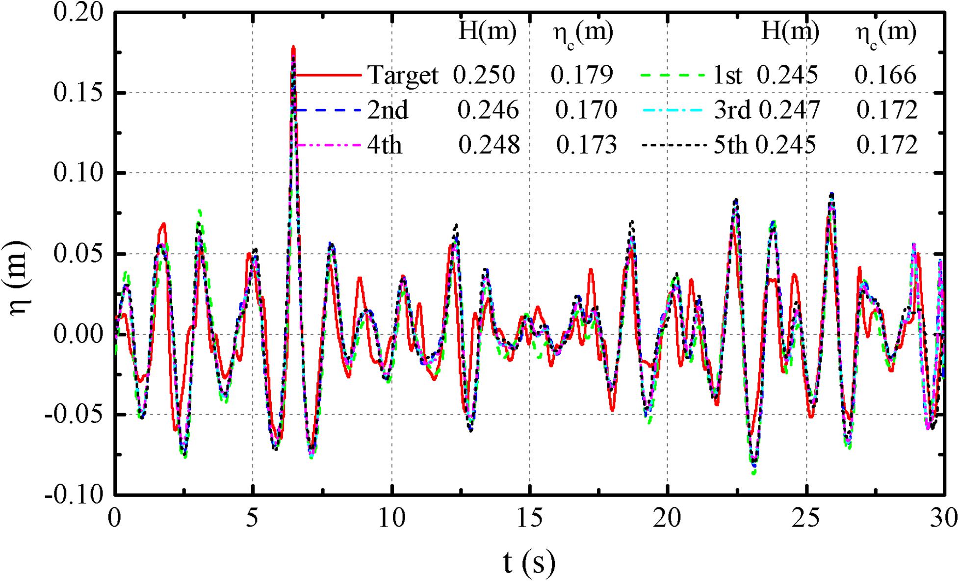
Figure 4. Comparison of the iterative modification results with the targets.

The wave elevations of the first-time modification result monitored at eleven positions are shown in Figure 5A, where 0 m corresponds with x = 7.3 m, A represents the difference between η_c and the wave front trough, which varies from the traditional definition of the wave height (H). The development process of the freak wave can be observed. η_c and A range from 0.145 to 0.177 m, and 0.219 to 0.266 m, where A is the wave front height. The maximum η_c and A occur at x = 0.3 and −0.1 m, respectively.

FIGURE 5

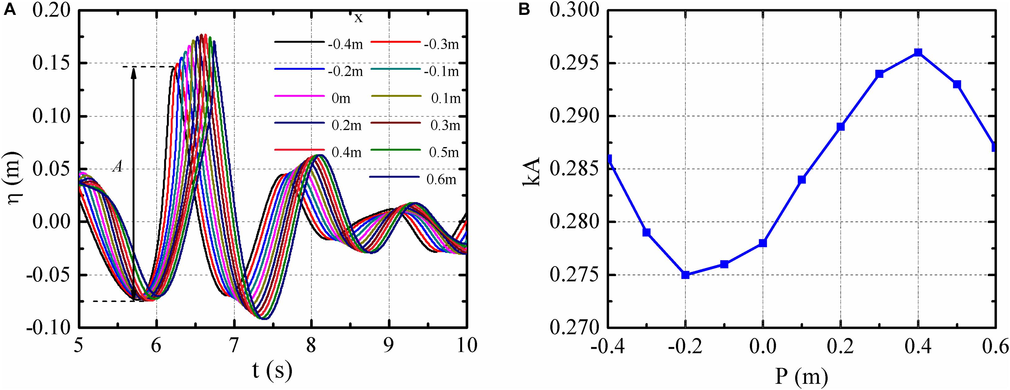
Figure 5. Wave elevation histories and wave front steepness kA at different locations. (A) Wave elevation histories, (B) wave front steepness kA at different locations.

The wave front steepness kA at different locations are shown in Figure 5B, where k is the wave number calculated by the trough-to-trough period of the freak wave. The maximum and minimum kA are 0.296 and 0.275, which occur at x = 0.4 and −0.2 m, respectively. Overall, the kA in this region are very close.

Action of the “NYW” on a Bottom-Mounted Vertical Cylinder

Empirical Formulations of Inline Forces

Morison formulation is used to calculating the inline force on the fixed unit length vertical cylinder, which can be presented as:

$$f_M(t,z)=\frac{1}{2}{C}_D\mathrm{\rho }D{u}_x(t,z)\left|u_x(t,z)\right|+C_M\mathrm{\rho }\frac{\mathrm{\pi }{D}^2}{4}\frac{d{u}_x(t,z)}{dt}(10)$$

where f_M is the wave force acting on unit length body, ρ is the water density, u_x is the horizontal water particle velocity, C_D, C_M are the empirical drag and inertial coefficients, which are selected as 1.0 and 2.0, respectively. However, the Morison formulation can be used only for the calculation of the linear harmonic force and it cannot be used for prediction of the high-order non-linear wave forces.

In order to refine the Morison inertia term, the formulations for the “axial divergence force” and “surface intersection force” on a slender body were proposed by Rainey (1995), which brings the accuracy up to the second-order in Stokes expansion. The corresponding correction terms to calculate the inline forces can be written as:

$$F_A={\displaystyle {\int }_{-d_s}^{\mathrm{\eta }}}\mathrm{\rho }{\displaystyle \frac{\mathrm{\pi }{D}^2}{4}}{u}_x\left({\displaystyle \frac{\partial u_z}{\partial z}}\right)\mathit{d}z(\mathrm{11a})$$

$$F_I=-({\displaystyle \frac{\mathrm{\pi }{D}^2}{4}})u_x^2{\displaystyle \frac{\partial \mathrm{\eta }}{\partial x}}(\mathrm{11b})$$

where the cylinder submerged depth (d_s) and wave surface elevation (η) are the lower and upper integral bounds for the “axial divergence force,” respectively. Eq. 11a is the second order in Stokes expansion and Eq. 11b represents a point force that exists at the instantaneous free-surface elevation due to the entry and exit forces. The summation of F_M, F_A, and F_I can be denoted as F_MAI, i.e., F_MAI = F_M+F_A+F_I.

3-D Numerical Simulation of the Inline Forces Induced by the “NYW”

The aforementioned wave generation method of the “NYW” was applied to the 3-D numerical wave tank, and modified the wavemaker control signal for one time. The cylinder is located at x = 7.3 m, and the diameter (D) and submerged depth (d_s) of the cylinder are 0.1 and 0.3 m, respectively. For the 3-D numerical model, the grids around the cylinder in the x-y plane are shown in Figure 6, where N_C, N_L, and N_Y are the cell numbers around the cylinder, body-fitted cell layers, and Y-axis grids, respectively. The simulation need to avoid the buffer layer while determining the y⁺(= $\frac{u^{*}y}{\upsilon }$, where u^∗ is the friction velocity; y is the wall spacing, and υ is the dynamic viscosity.), which in other words is to guarantee either y⁺ < 5 (viscous sublayer) or 300 > y⁺ > 30 (logarithmic sublayer), and y+ were kept inside this region (300 > y⁺ > 30) for all the simulations in the present study. The maximum dimensionless wall distance y⁺ of the first layer grids was lower than 100.

FIGURE 6

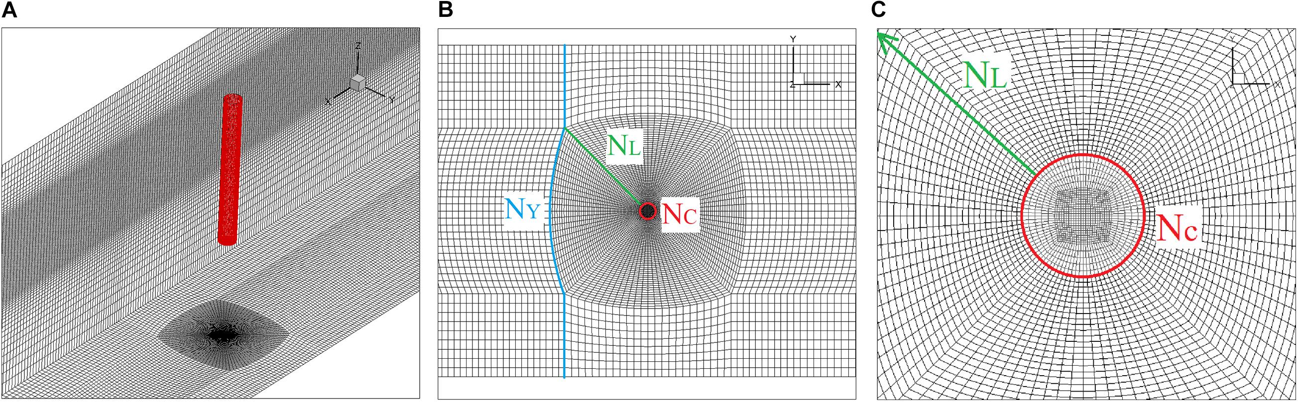
Figure 6. Overall and detailed mesh arrangements. (A) Global mesh, (B) local mesh around the cylinder, and (C) zoomed local mesh.

In order to further study the influences of the mesh arrangement around the cylinder on the evaluate inline forces accuracy, a mesh convergence study on the 3-D numerical model was carried out, and the grid parameters are listed in Table 2. All of the cases in this study were computed on a workstation with 4 × Intel(R) Xeon 6148 CPUs.

TABLE 2

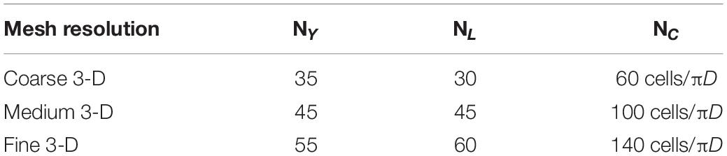
Table 2. Grid parameters for mesh convergence study of the 3-D model.

The actions of the “NYW” on a bottom-mounted vertical cylinder with different grid numbers are shown in Figure 7A. Generally, the results from Medium and Fine meshes are fairly close, and the Medium (3-D) mesh is adopted for the following analysis in consideration of both simulation accuracy and computation time. Based on the numerically simulated wave elevations, the FFT decomposition was performed to obtain the related linear wave components, including the component wave numbers, amplitudes and the initial phases. For an irregular wave series, a common practice is to superimpose water velocity and acceleration of each wave component. The F_M, F_MAI, and experimental results (Deng et al., 2016) are also shown in Figure 7A for comparisons. Some findings can be summarized as follows:

FIGURE 7

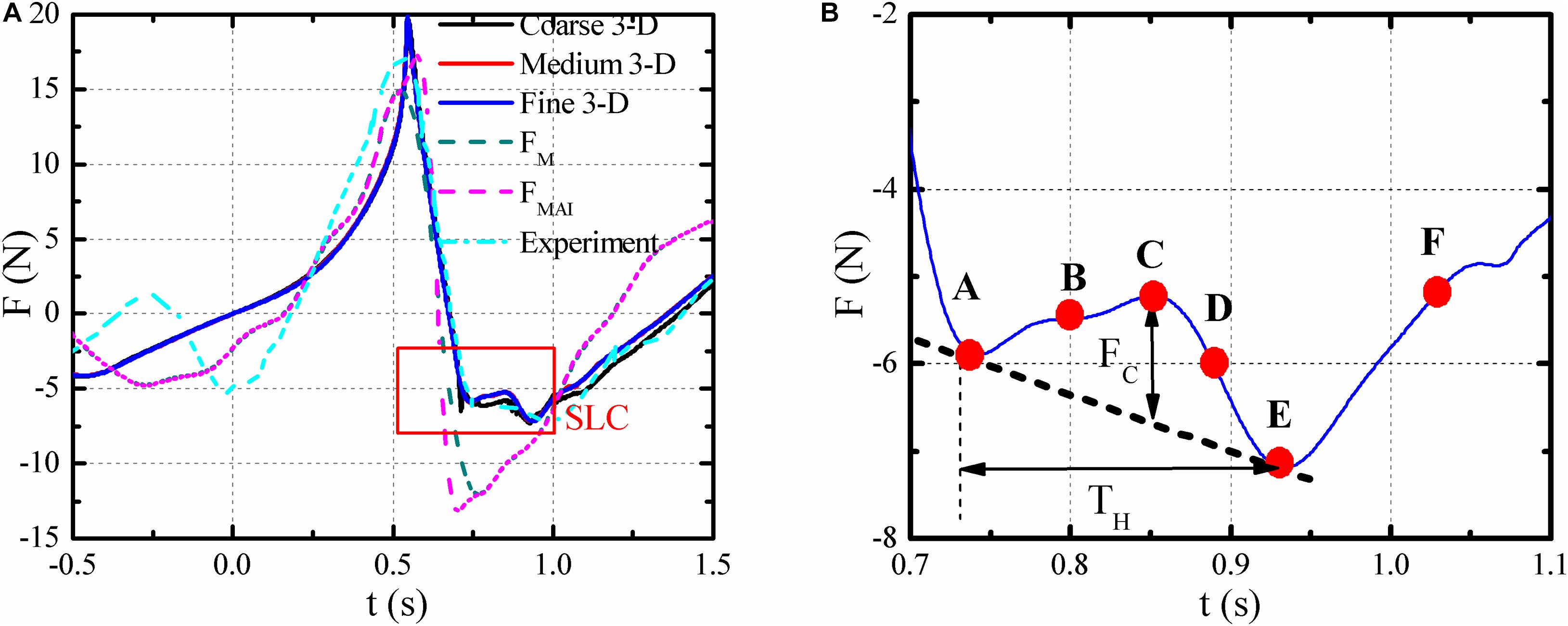
Figure 7. Inline forces acting on the cylinder. (A) Inline forces, (B) numerical results of the SLC.

(1) Because the Morison formulation cannot accurately calculate the high-order non-linear wave forces, the maximum F_M is smaller than those of the numerical and experimental cases. F_MAI improves the accuracy to the second-order in Stokes expansion, and the peak result is closer to the numerical value. As shown in Figure 7A, both F_M and F_MAI deviate from the numerical and experimental results with SLC, it should be stated that the SLC stage can be predicted by neither F_M and nor F_MAI.

(2) The numerically simulated inline forces histories are fairly close to the experimental results. The differences are mainly due to the different target wave elevations. The target in the experiment was derived from the JONSWAP spectrum, which unavoidably deviates much or less from the actual “NYW” series. H and η_c in the experiment are also smaller than those of the numerical simulation.

Analyses of the SLC

The SLC, which is an additional longitudinal short-duration force prior to the minimum wave force, may appear when a steep crest passes the vertical cylinder, and it was firstly identified by Grue et al. (1993). The wave forces that calculated by the theoretical methods (e.g., Morison formulation, slender body theory, and FNV) have some weaknesses in predicting the inline forces, especially for the minimum forces and SLC stage. Compared with the experimental method, the computational fluid dynamics (CFD) methods have some superiorities in revealing the mechanism of SLC of vertical cylinders, because more flow details around the structure can be obtained. For the SLC, F′_c (= F_ck/ρgπr²) and F_c/F_p were respectively used by Chaplin et al. (1997) and Liu et al. (2019) to quantify the magnitude of SLC, where F_p is the peak-to-peak value of the total inline wave force, F_c is shown in Figure 7B. The F′_c and F_c/F_p are 0.043 and 0.053, respectively. In addition, the dimensionless parameter T′_H (= T_H/T) was used to quantify the duration of the SLC, where T_H is the duration of SLC, and the T′_H = 0.152 in this case.

Paulsen et al. (2014) numerically studied the SLC of bottom-mounted cylinders under regular waves conditions, the downstream vortex was observed in the SLC cases. However, the detailed relationship between the downstream vortex and the SLC was not unveiled. In this study, six typical moments were selected, which were marked as A–F in Figure 7B, to investigate the effects of the vortices on the SLC. The instantaneous flow fields in the slice of z = 0.75 m are shown in Figure 8A. As the vortex structures in the SLC stage remain symmetric, the wall pressure distributions also keep symmetry along the wave propagating direction, so the side-wall pressure distribution is shown in Figure 8B.

FIGURE 8

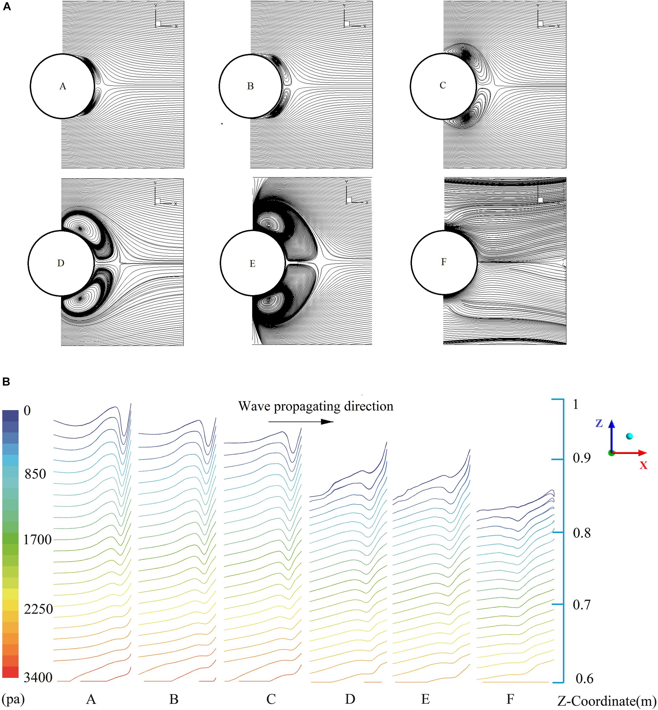
Figure 8. Downstream vortices and side-wall pressure distribution during SLC. (A) downstream vortices, (B) pressure contour lines on the side-wall surface.

Two symmetric vortices appear at moment A, the wall pressure shows visible changes near the position of the downstream vortices, the non-smoothed pressure contour line indicates that the wall pressures decrease in those areas. Then the downstream vortices become larger and the influences on the side-wall pressure are more notable. The influences of the vortical structures on the wall pressure becomes more significant with decreasing submerged depths. The inline force continues to decrease with the rising of vortex size, and the inline force is slightly upward during the moment A–C. The downstream vortices become largest at moment E and move from the downstream to the lateral sides of the cylinder. At the same time, the nonsmoothed pressure contour line also moves to the side of the cylinder. At moment F, the vortices structures disappeared and the pressure changes become less pronounced. According to the relationships between the development of SLC and the vortex processes, it can be inferred that the downstream vortices lead to the decrease of wall pressures, which may be the main cause of SLC.

Figure 9 presents the flow velocity distributions along the z-direction with 0.5r, r, and 1.5r (r is the radius of the cylinder) downstream the cylinder. At Moment A, the return flow was observed at position 0.5r, the velocity changes more obviously with the increase in the z coordinate, which induced the wall pressure changes more notably near the water surface. Then the range of the return flow area becomes larger with the development of SLC, and the return flow was observed at positions 0.5r, r, and 1.5r. As shown in Figure 9, it indicates that the return flow is induced by the downstream vortex, and larger vortices will produce more distinct effects on the flow velocity, which finally results in the SLC (additional inline forces). According to the analysis of the numerical computations, the SLC may be induced by downstream vortex associated with the changes of the wall pressure and return flow.

FIGURE 9

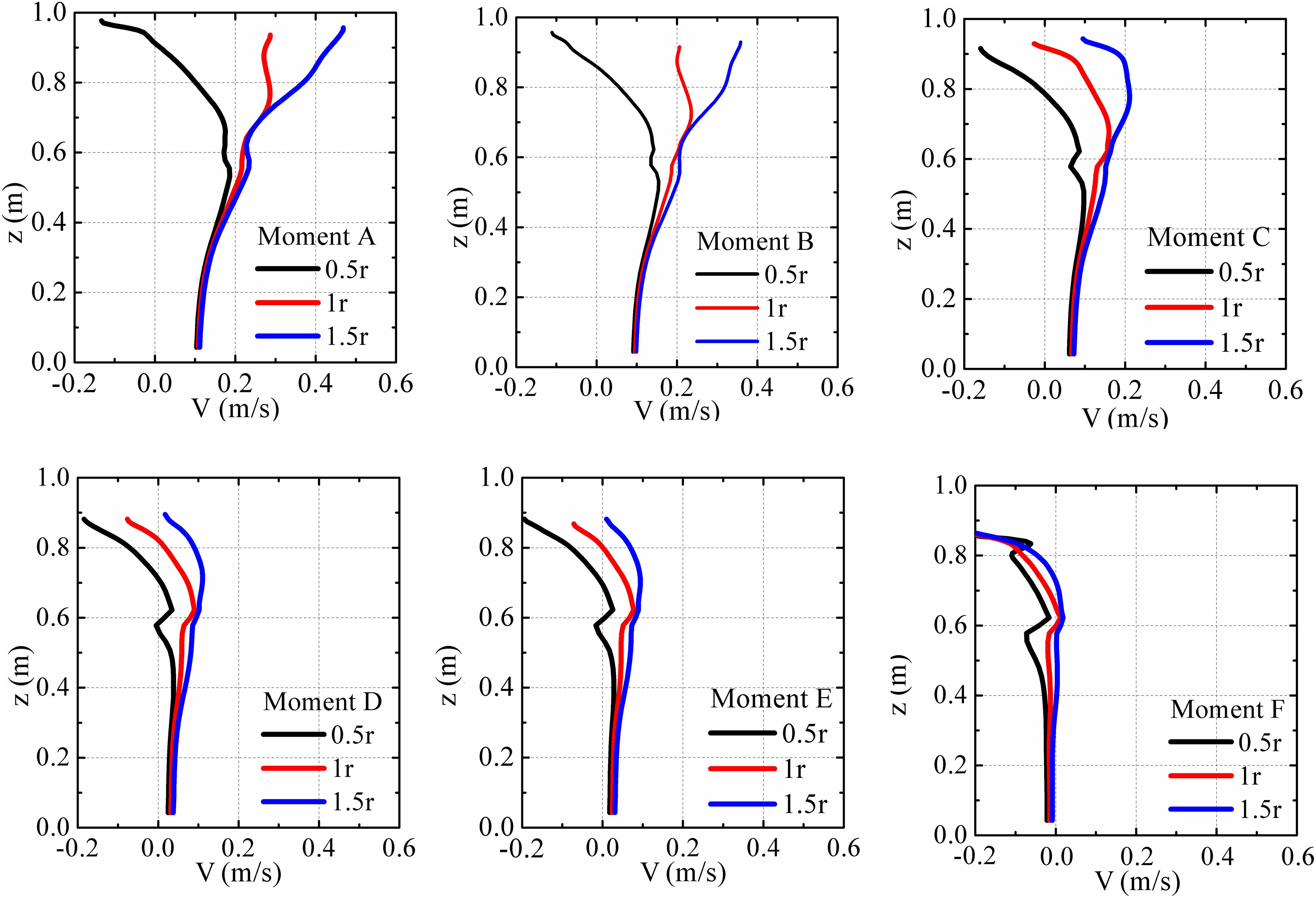
Figure 9. Distributions of flow velocity during SLC.

Inline Forces With Different Cylinder Positions

In order to study the effects of kA on the maximun inline forces and the magnitude of the SLC. Seven more cases with different cylinder locations, i.e., x = −0.2, −0.1, 0.1, 0.2, 0.3, 0.4, and 0.5 m were calculated. The time histories of inline forces are shown in Figure 10. The related maximum inline forces are listed in Table 3, where the dimensionless parameter kA could be obtained from Figure 5B.

FIGURE 10

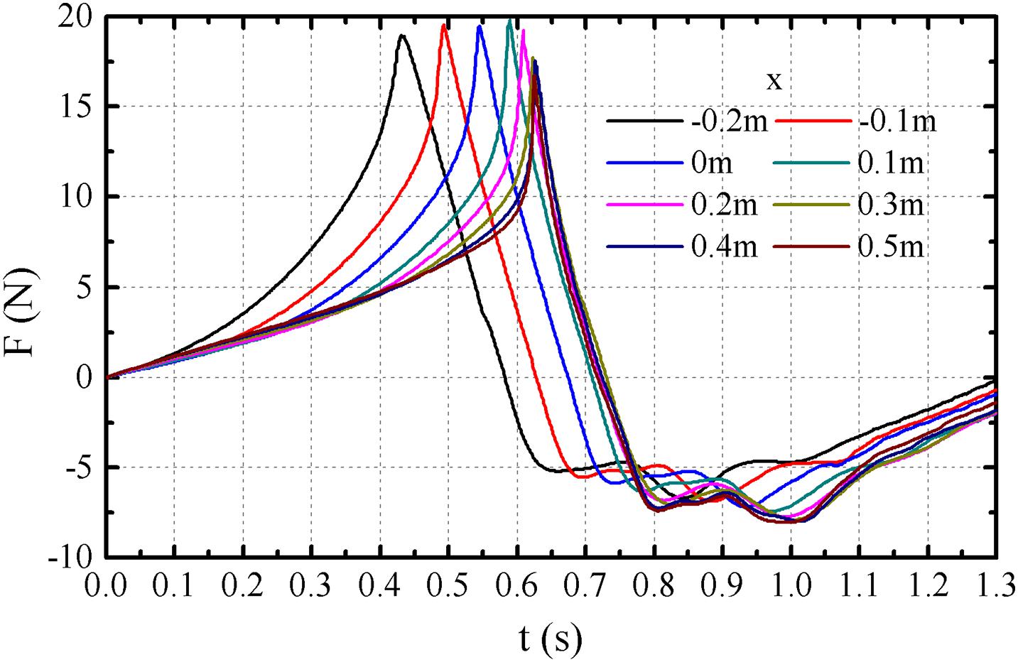
Figure 10. Inline forces at different positions.

TABLE 3

Table 3. Maximum inline forces on cylinders at different positions.

It found that the F_CFD/F_M and F_CFD/F_MAI increase with increasing the kA, which indicates the occupation of the non-linear components correspondingly become larger. According to the results of F_CFD/F_M, the ratio of linear inline force to the total is less than 65% when kA equals to 0.296. For the inline forces induced by the freak waves, such as the “NYW,” both F_M and F_MAI would underestimate the maximum inline forces that contain the higher-order components and slamming forces. Besides, the maximum forces occurred before the wave crest and the delta-T among the range from 0.08 to 0.11 s for the eight cases, which are close to the experimental results (Deng et al., 2016). Based on the numerical results, the moment of the force peak is not the instant when the still water passes through the central axis of the cylinder. Therefore, it is inappropriate to predict the moment of the maximum wave force through the regular wave theory.

As shown in Figure 11, F′_c and F_c/F_p vary from 3.3 to 4.3%, and 4.3 to 5.4%, respectively. F′_c decreases with increasing kA when kA is larger than 0.276. The dimensionless parameter T′_H varies from 0.127 to 0.140, which show fairly satisfactory agreements with the values (T′_H < 0.150 and <0.173) that were respectively monitored by Grue et al. (1993) and Liu et al. (2019).

FIGURE 11

Figure 11. The relationship between F′_c, F_c/F_p, and kA.

Considering the SLC is a complex phenomenon, the kA in the aforementioned 3-D cases were relatively close, more focused wave cases were numerically simulated to further study the influence of the flow fields on the wave forces. The focused waves for C745, C765, and C775 in the experiments of Chaplin et al. (1997) were simulated. The related parameters of the three waves could be obtain from the descriptions for the focused waves (Chaplin et al., 1997). The still water depth was 0.525 m and the duration between troughs was close to 1.1 s.

As mentioned in the experiment, the focused wave series was generated by the superposition of 34 simple harmonic wave components, the frequencies of which ranged from 0.511 to 1.244 Hz, with a step of 0.0222 Hz. Same with the generation of the NYW, the superposition of the simple harmonics (Longuet-Higgins, 1974) was taken as the target of the numerical simulation. The numerically simulated wave series are shown in Figure 12A, and the experimental results are also offered for comparison. The simulated wave height and wave crest coincide well with those of the experimental results.

FIGURE 12

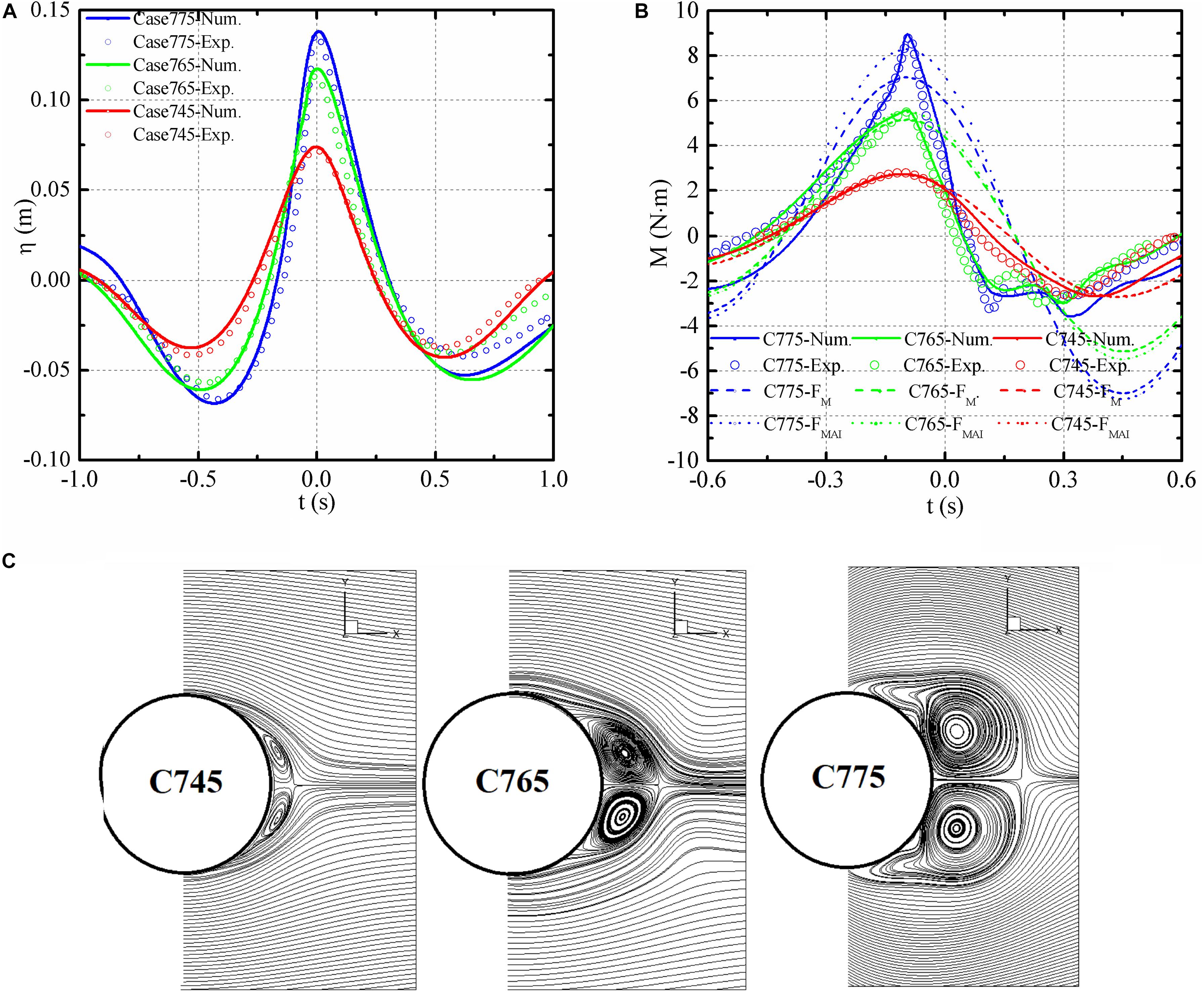
Figure 12. Simulation results for the focused wave cases. (A) Wave elevations, (B) overturning moments, and (C) velocity streamlines at z = 0.425 m.

Based on the experiments conducted by Chaplin et al. (1997), the vertical cylinder was located in the center of the working zone, which the diameter is 100 mm. The numerical and experimental overturning moments are shown in Figure 12B. Overall, the two sets of histories match fairly well, especially for the maximum moments. For the cases with smaller wave steepness, the F_M and F_MAI could predict the maximum overturning moments accurately, but both the Morison formula and the slender body theory would underestimate the maximum overturning moments when the wave steepness becomes larger. Similar to the results in Figure 7A, the maximum M_M is smaller than those of the numerical and experimental cases. M_MAI improves the accuracy to the second-order in Stokes expansion, and the peak result is closer to the numerical and experimental values. In addition, the SLC appeared for C765 and C775, whereas it was not observed for C745. Those existing theoretical formula could not predict SLC stage, because those formulas considered the fluid is idealized and assumed to be irrotational and non-viscous, therefore, the suction forced induced by the downstream vortex could not be monitored. Moreover, the CFD method could predict the SLC stage satisfactorily, this also verified the numerical simulation accuracy.

The horizontal velocity streamlines at Moment E are shown in Figure 12C, in which the velocity streamlines are in a horizontal plane perpendicular to the axis of the cylinder for z = 0.425 m. For C765 and C775, two symmetric vortices were generated on the near-wall surfaces of both sides of the cylinder during the SLC stage. In comparison, the vortices in C745 were much smaller. The corresponding magnitudes of the SLC, F′_c of C745, C765, and C775 were 0, 0.044, and 0.059, respectively. Thus, the vortex size is one important factor affecting the magnitude of the SLC.

Concluding Remarks

The “NYW” was numerically simulated based on the 2-D CFD model and the modification method was applied to improve the simulation accuracy. In addition, the action of the “NYW” on a bottom-mounted vertical cylinder was numerically simulated based on the 3-D model. Sensitivity analysis for the grid resolution was conducted to ensure the computational accuracy, and the simulation results were compared with the experimental and empirical formulation results, the differences were analyzed to unveil the possible causes. Finally, the influences of kA on the maximum inline forces were analyzed. Some major conclusions are drawn as follows:

(1) For the simulation of the extreme freak wave, e.g., “NYW,” the simulation accuracy can be improved by the compensation for the difference between the target wave series and initial numerical results.

(2) Under the action of “NYW,” the cylinder maximum and minimum inline forces including the high-order non-linear components cannot be accurately predicted by the Morison and the slender body theoretical formulations. In addition, the pressure contour line and distribution of velocities at six typical moments during the SLC stage shows that the appearance of SLC is closely related to the downstream vortex, the vortex size is one important factor affecting the magnitude of the SLC.

(3) The non-linear components of the inline force increase with increasing kA. The numerical results reveal that the linear inline force may be less than 65% of the total wave loading. The Morison and slender body theoretical formulations would underestimate the maximum inline forces that contain the higher-order components andslamming forces. This paper provides a useful reference for the design of the support structures for TLPs and monopile foundations of the OWTs under the actions of the freak waves.

Data Availability Statement

The raw data supporting the conclusions of this article will be made available by the authors, without undue reservation.

Author Contributions

YW: methodology, formal analysis, data curation, and writing-original draft. FX: conceptualization, supervision, resources, writing-review and editing, and visualization. ZZ: software and validation. All authors contributed to the article and approved the submitted version.

Funding

This work is supported by the National Science Foundation of China (51978130). The authors would like to sincerely thank Sverre Haver from Statoil for providing the New Year Wave series.

Conflict of Interest

The authors declare that the research was conducted in the absence of any commercial or financial relationships that could be construed as a potential conflict of interest.

References

Bachynski, E. E., and Moan, T. (2014). Ringing loads on tension leg platform wind turbines. Ocean Eng. 84, 237–248. doi: 10.1016/j.oceaneng.2014.04.007

CrossRef Full Text | Google Scholar

Bertotti, L., and Cavaleri, L. (2008). Analysis of the Voyager storm. Ocean Eng. 35, 1–5. doi: 10.1016/j.oceaneng.2007.05.008

CrossRef Full Text | Google Scholar

Bredmose, H., and Jacobsen, N. G. (2010). “Breaking wave impacts on offshore wind turbine foundations: focused wave groups and CFD,” in Proceedings Of The Asme 2010 29th International Conference On Ocean, Offshore And Arctic Engineering, (New York: ASME).

Google Scholar

Chaplin, J. R. (1996). On frequency-focusing unidirectional waves. Int. J. Offsh. Polar Engin. 6, 131–137.

Google Scholar

Chaplin, J. R., Rainey, R. C. T., and Yemm, R. W. (1997). Ringing of a vertical cylinder in waves. J. Fluid Mech. 350, 119–147. doi: 10.1017/s002211209700699x

CrossRef Full Text | Google Scholar

Chen, L. F., Zang, J., Taylor, P. H., Sun, L., Morgan, G., Grice, J., et al. (2018). An experimental decomposition of nonlinear forces on a surface-piercing column: Stokes-type expansions of the force harmonics. J. Fluid Mech. 848, 42–77. doi: 10.1017/jfm.2018.339

CrossRef Full Text | Google Scholar

Deng, Y., Yang, J., Zhao, W., Li, X., and Xiao, L. (2016). Freak wave forces on a vertical cylinder. Coast Eng. 114, 9–18. doi: 10.1016/j.coastaleng.2016.03.007

CrossRef Full Text | Google Scholar

Deng, Y., Yang, J., Zhao, W., Xiao, L., and Li, X. (2015). An efficient focusing model of freak wave generation considering wave reflection effects. Ocean Eng. 105, 125–135. doi: 10.1016/j.oceaneng.2015.04.058

CrossRef Full Text | Google Scholar

Faltinsen, O. M., Newman, J. N., and Vinje, T. (1995). Nonlinear wave loads on a slender vertical cylinder. J. Fluid Mech. 289, 179–198. doi: 10.1017/s0022112095001297

CrossRef Full Text | Google Scholar

Gao, N., Yang, J., Zhao, W., and Xin, L. (2015). Numerical simulation of deterministic freak wave sequences and wave-structure interaction. Ships Offsh. Struct. 11, 1–16.

Google Scholar

Ghadirian, A., Bredmose, H., and Dixen, M. (2016). Breaking phase focused wave group loads on offshore wind turbine monopiles. Proc. J. Phys. 753:2016.

Google Scholar

Grue, J., Gunnhild, B., and Øyvind, S. (1993). Higher harmonic wave exciting forces on a vertical cylinder. Mech. Appl. Math. 1993, 1–30.

Google Scholar

Haver, S. (2003). Freak wave event at Draupner jacket January 1 1995. Statoil Technical Report. Netherland: Springer.

Google Scholar

Hirt, C. W., and Nichols, B. D. (1981). Volume of fluid (VOF) method for the dynamics of free boundaries ⋆. J. Comput. Phys. 39, 201–225. doi: 10.1016/0021-9991(81)90145-5

CrossRef Full Text | Google Scholar

Kharif, C., and Pelinovsky, E. (2003). Physical Mechanisms of the Rogue Wave Phenomenon. Eur. J. Mech. B Fluid 22, 603–634. doi: 10.1016/j.euromechflu.2003.09.002

CrossRef Full Text | Google Scholar

Kharif, C., Pelinovsky, E., and Slunyaev, A. (2009). Rogue waves in the ocean. Netherland: Springer Science & Business Media.

Google Scholar

Kim, J., O Sullivan, J., and Read, A. (2012). “Ringing analysis of a vertical cylinder by Euler overlay method,” in Proceedings Of The Asme 31st International Conference On Ocean, Offshore And Arctic Engineering, (New York: ASME).

Google Scholar

Klinting, P., and Sand, S. E. (1987). Analysis of Prototype Freak Waves, SCE Special Conference Nearshore Hydrodynamics. Hoersholm: Dansk Hydraulisk Ins, 618–632.

Google Scholar

Kriebel, D. L., and Alsina, M. V. (2000). “Simulation of extreme waves in a background random sea,” in Proceedings of the Tenth International Offshore and Polar Engineering Conference, (United State: International Society of Offshore and Polar Engineers).

Google Scholar

Liu, S., Jose, J., Ong, M. C., and Gudmestad, O. T. (2019). Characteristics of higher-harmonic breaking wave forces and secondary load cycles on a single vertical circular cylinder at different Froude numbers. Mar. Struct. 64, 54–77. doi: 10.1016/j.marstruc.2018.10.007

CrossRef Full Text | Google Scholar

Longuet-Higgins, M. S. (1974). “Breaking waves in deep or shallow water,” in Proceedings of the Proc. 10th Conf. on Naval Hydrodynamics, (New York: Springer).

Google Scholar

Molin, B. (1995). Third-harmonic wave diffraction by a vertical cylinder.. J Fluid Mech. 302, 203–229. doi: 10.1017/s0022112095004071

CrossRef Full Text | Google Scholar

Morison, J. R., Johnson, J. W., and Schaaf, S. A. (1950). The force exerted by surface waves on piles. J. Petrol. Technol. 2, 149–154. doi: 10.2118/950149-g

PubMed Abstract | CrossRef Full Text | Google Scholar

Ning, D. Z., Teng, B., Taylor, R. E., and Zang, J. (2008). Numerical simulation of non-linear regular and focused waves in an infinite water-depth. Ocean Eng. 35, 887–899. doi: 10.1016/j.oceaneng.2008.01.015

CrossRef Full Text | Google Scholar

Ning, D., Wang, R., Chen, L., Li, J., Zang, J., Cheng, L., et al. (2017). Extreme wave run-up and pressure on a vertical seawall. Appl. Ocean Res. 67, 188–200. doi: 10.1016/j.apor.2017.07.015

CrossRef Full Text | Google Scholar

Pakozdi, C., östman, A., Bachynski, E. E., and Stansberg, C. T. (2016). “CFD reproduction of model test generated extreme irregular wave events and nonlinear loads on a vertical column,” in Proceedings of the ASME 2016 35th International Conference on Ocean, Offshore and Arctic Engineering, (New York: ASME).

Google Scholar

Paulsen, B. T., Bredmose, H., Bingham, H. B., and Jacobsen, N. G. (2014). Forcing of a bottom-mounted circular cylinder by steep regular water waves at finite depth. J. Fluid Mech. 755, 1–34. doi: 10.1017/jfm.2014.386

CrossRef Full Text | Google Scholar

Rainey, R. (1995). Slender-body expressions for the wave load on offshore structures. Proc. Roy. Soc. London. Ser A 450, 391–416. doi: 10.1098/rspa.1995.0091

CrossRef Full Text | Google Scholar

Rainey, R. (2007). Weak or strong nonlinearity: the vital issue. J. Eng. Math. 58, 229–249. doi: 10.1007/s10665-006-9126-2

CrossRef Full Text | Google Scholar

Tang, Y., Shi, W., Ning, D., You, J., and Michailides, C. (2020). Effects of Spilling and Plunging Type Breaking Waves Acting on Large Monopile Offshore Wind Turbines. Front. Mar. Sci. 7:427.

Google Scholar

Tromans, P. S., Anaturk, A. R., and Hagemeijer, P. (1991). “A new model for the kinematics of large ocean waves-application as a design wave,” in Proceedings of the First International Offshore and Polar Engineering Conference, (United State: International Society of Offshore and Polar Engineers).

Google Scholar