 April B. Cook1*
 Andrea M. Bernard1
 Kevin M. Boswell2
 Heather Bracken-Grissom2
 Marta D’Elia2
 Sergio deRada3
 Cole G. Easson1,4
 David English5
 Ron I. Eytan6
 Tamara Frank1
 Chuanmin Hu5
 Matthew W. Johnston1
 Heather Judkins7Chad Lembke5
 Jose V. Lopez1
 Rosanna J. Milligan1
 Jon A. Moore8,9
 Bradley Penta3
 Nina M. Pruzinsky1John A. Quinlan10
 Travis M. Richards6
 Isabel C. Romero5
 Mahmood S. Shivji1
 Michael Vecchione11
 Max D. Weber6
 R. J. David Wells6
 Tracey T. Sutton1
- 1Guy Harvey Oceanographic Center, Halmos College of Arts and Sciences, Nova Southeastern University, Dania Beach, FL, United States
- 2Institute of Environment, Department of Biological Sciences, Florida International University – Biscayne Bay Campus, North Miami, FL, United States
- 3United States Naval Research Laboratory, Stennis Space Center, Washington DC, United States
- 4Department of Biology, Middle Tennessee State University, Murfreesboro, TN, United States
- 5College of Marine Science, University of South Florida, Tampa, FL, United States
- 6Department of Marine Biology, Texas A&M University at Galveston, Galveston, TX, United States
- 7Integrative Biology, University of South Florida St. Petersburg, St. Petersburg, FL, United States
- 8Wilkes Honors College, Florida Atlantic University, Jupiter, FL, United States
- 9Florida Atlantic University, Harbor Branch Oceanographic Institute, Fort Pierce, FL, United States
- 10Southeast Fisheries Science Center, National Oceanic and Atmospheric Administration, Miami, FL, United States
- 11NMFS National Systematics Laboratory, National Museum of Natural History, Washington, DC, United States
The pelagic Gulf of Mexico (GoM) is a complex system of dynamic physical oceanography (western boundary current, mesoscale eddies), high biological diversity, and community integration via diel vertical migration and lateral advection. Humans also heavily utilize this system, including its deep-sea components, for resource extraction, shipping, tourism, and other commercial activity. This utilization has had impacts, some with disastrous consequences. The Deepwater Horizon oil spill (DWHOS) occurred at a depth of ∼1500 m (Macondo wellhead), creating a persistent and toxic mixture of hydrocarbons and dispersant in the deep-pelagic (water column below 200 m depth) habitat. In order to assess the impacts of the DWHOS on this habitat, two large-scale research programs, described herein, were designed and executed. These programs, ONSAP and DEEPEND, aimed to quantitatively characterize the oceanic ecosystem of the northern GoM and to establish a time-series with which natural and anthropogenic changes could be detected. The approach was multi-disciplinary in nature and included in situ sampling, acoustic sensing, water column profiling and sampling, satellite remote sensing, AUV sensing, numerical modeling, genetic sequencing, and biogeochemical analyses. The synergy of these methodologies has provided new and unprecedented perspectives of an oceanic ecosystem with respect to composition, connectivity, drivers, and variability.
Introduction
Of the ecotypes of the Gulf of Mexico (GoM) affected by the Deepwater Horizon oil spill (DWHOS), the open-ocean pelagic ecotype was by far the largest. The spill began on April 20, 2010, about 66 km off the coast of Louisiana, at a depth ∼1,500 m and continued for 87 days (Beyer et al., 2016). Some percentage of oil, other hydrocarbons, and injected dispersant reached the sea surface and seabed, whereas 100% occurred within the deep-pelagic domain (200 m depth to just above the seafloor). During the summer of 2010, a continuous plume of oil over 35 km in length was discovered at approximately 1,100 m depth (Camilli et al., 2010). This plume persisted for several months, prompting concern about the effects of the DWHOS on the meso- and bathypelagic (200–1000 and >1,000 m depths, respectively; deep-pelagic, cumulatively) faunas. Deep-pelagic animals are known to vertically migrate to shallow, epipelagic (0–200 m depth) waters at night to feed (Sutton et al., 2020), a process which ostensibly increases exposure throughout the water column and connects the shallower and deeper parts of the oceanic GoM.
Gaining insight and understanding of pelagic ecosystems over time requires a multidisciplinary approach, given their complex physical (4-D, Lagrangian), biological, and ethological (vertically migratory) nature. Here we describe the sampling, sensing, and analysis methods of two major research programs, both aimed at characterizing effects, or potential effects, of the DWHOS on the epi-, meso-, and bathypelagic faunas of the northern GoM. The first program, ONSAP (Offshore Nekton Sampling and Analysis Program), was supported by the National Oceanic and Atmospheric Administration (NOAA) as part of the DWHOS Natural Resource Damage Assessment (NRDA) conducted in 2010–2015. This program encompassed in situ net sampling, water column profiling, and active acoustic sensing (Supplementary Tables 1,2) to address the question, “What could have been affected by the DWHOS in the deep-pelagic GoM?” The dearth/lack of pre-DWHOS data and the needs of the NRDA process required this initial approach. The second program was DEEPEND (DEEp PElagic Nekton Dynamics), a research consortium supported by The Gulf of Mexico Research Initiative (GoMRI) from 2015 to 2020. This program, which added satellite remote sensing, AUV sensing, physical oceanographic numerical modeling, pelagic microbial ecology, genetic analysis, biogeochemical analysis, and trophic ecology (Supplementary Tables 3,4) was both a continuation and evolution of ONSAP. The additions to DEEPEND, when integrated with foundational information from ONSAP, addressed the questions, “What are the natural drivers of pelagic ecosystem structure in the GoM?” and “Did pelagic faunal abundance variations after DWHOS exceed this ‘natural envelope’?”
Survey Approach
The overall goal of the initial ONSAP project was to survey and quantify the deep-pelagic life forms living within or traveling through the area of the GoM affected by the oil spill (Frank et al., 2020; Sutton et al., 2020). Of interest was the water column fauna at the mesopelagic/bathypelagic interface, the depth stratum containing the deep hydrocarbon plume. The plume was discovered in areas surrounding the Macondo wellhead where the spill originated. To accomplish this goal, a multi-disciplinary approach was used. Acoustic profiles were collected to synoptically quantify organisms distributed throughout the water column. These can easily be repeated for comparisons across space and time. While a very useful tool, acoustics cannot discern between individual species nor can it detect many deep-pelagic organisms without swim bladders or air pockets. Discrete-depth midwater trawling was conducted to identify and quantify the organisms collected during both day and night to account for vertical migration. These results also help to ground truth the acoustic profiles. Environmental factors such as temperature, conductivity, and dissolved oxygen were collected from both trawl-mounted sensors and CTD rosette profiling from 0 to 1500 m depth. Details of survey design and methodologies are described further below.
When planning the DEEPEND program, several additional components were added to the survey approach to fill in data gaps and to expand on research objectives. A remote sensing and satellite imagery component was added to identify mesoscale oceanographic and riverine discharge features to inform planning and execution of field work (e.g., Androulidakis et al., 2019). A glider was deployed to collect oceanographic data that were assimilated in the ocean model which was used to establish DEEPEND cruise tracks. This multidisciplinary methodology, integrating physical oceanographic modeling, satellite observation, and in situ sensing, provided the spatiotemporal habitat context by which pelagic faunal composition, abundance and distribution were analyzed (i.e., biophysical coupling; Meinert et al., 2020; Milligan and Sutton, 2020; Pruzinsky et al., 2020).
A biogeochemical component was added to directly measure the amount of petrogenic contamination in animal organs, muscle tissues, and eggs using polycyclic aromatic hydrocarbons (PAHs) as a proxy (Romero et al., 2018, 2020). A molecular taxonomy component (DNA barcoding; Hebert et al., 2003) was added to help identify damaged, cryptic, and juvenile specimens where morphological characters do not yet exist or could not differentiate between species (e.g., Moore et al., 2020). The gene sequences analyzed are well established as robust markers for species identification of marine fishes (Ward et al., 2009) and invertebrates (Mantelatto et al., 2018). A population genomics component was added (double-digest Restriction Associated DNA sequencing; ddRADseq) to study genetic diversity and connectivity of the GoM and adjacent water deep-pelagic fauna (Timm et al., 2020b). Genetic diversity and connectivity can be used as proxies to measure population health and resilience (Oliver et al., 2015). Over a time-series, these measures can show how diversity is maintained and restored in the face of anthropogenic and/or natural disasters. A trophic ecology component, using Stable isotope analysis (SIA), was added to identify feeding relationships among taxa, estimate trophic positions, and delineate energy flow (Richards et al., 2020). Understanding the flow of energy through this deep-sea ecosystem is essential to be able to identify linkages which may be vulnerable to disasters such as an oil spill. A microbial ecology component was added to help characterize pelagic habitats (along with environmental and ocean modeling data) and to investigate the dynamics of diel vertical migration using acoustic backscatter data and eDNA sampling (Easson et al., 2020).
The time-series aspect of these two programs provides information on the patterns of abundance and distribution of the pelagic fauna, the concentration of PAHs therein, and the pattern of genetic diversity following a major marine disaster. Information such as this also provides a basis against which to compare hindcast-derived abundance estimates using proxies for data that did not previously exist (e.g., larval and adult deep-pelagic fish abundance relationships; the former data were collected prior to the DWHOS, while the latter were not). The multidisciplinary nature of these two programs facilitates an ecosystem-based approach to guide interpretations of assemblage-level data. For example, using ddRADseq in combination with physical oceanographic modeling provided evidence that the Loop Current could be facilitating genetic connectivity in pelagic shrimps, with its concomitant implications for the recovery and resilience of a species (Timm et al., 2020a). In another example, microbial assemblages were characterized using abiotic and biotic data collected via CTD sensing and their dynamics interpreted using MODIS satellite imagery (Easson and Lopez, 2019). In summary, results derived from each component were valuable in their own right, but each also added necessary information for other working groups.
Transect Design
During ONSAP field operations, a subset of the Southeast Area Monitoring and Assessment Program (SEAMAP; Eldridge, 1988) stations surrounding the DWHOS site was sampled (Figure 1), with original station nomenclature maintained. Sampling the entire 46-station grid took approximately 3 months, requiring that sampling be divided into several legs for resupply and personnel changes. This necessity dictated that sampling transects be arranged by logistics (time to station, weather, and personnel availability) in lieu of oceanographic and/or ecological considerations. Sampling, acoustic sensing, and water column profiling were conducted twice at each station (day and night). Sampling of the entire grid was conducted three times over a 9-month period, with each station being occupied either three (most stations) or two times over the course of ONSAP (Figure 1).
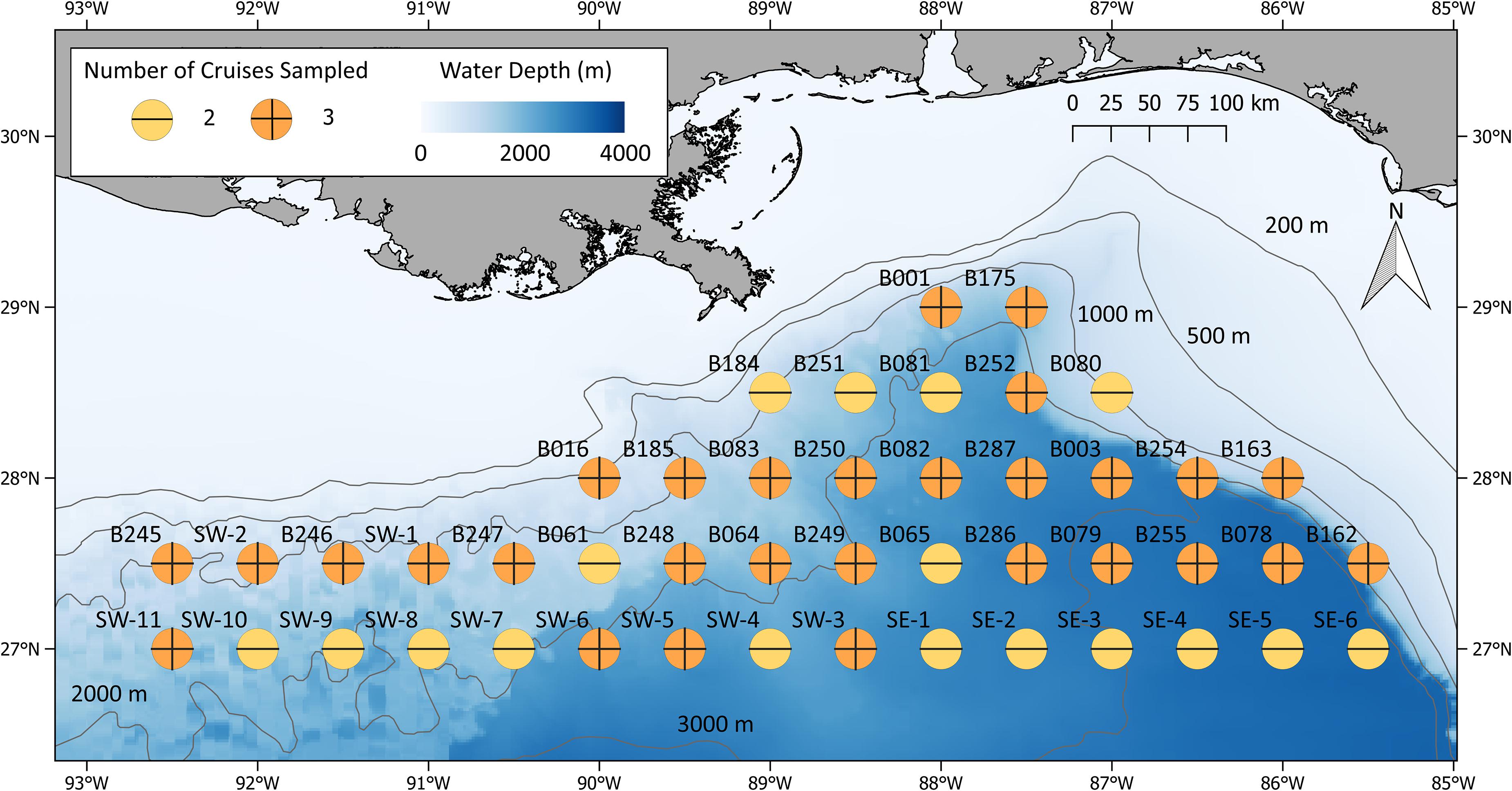
Figure 1. ONSAP MOC10 stations sampled during the winter, spring, and summer 2011. Symbol colors represent the number of seasons (up to three) each location was sampled.
Due to time constraints, only a portion of the stations sampled during ONSAP were sampled during individual DEEPEND cruises, each of which lasted approximately 15 days. DEEPEND cruise tracks were designed to transect as many water masses (Common Water and Loop Current, sensu Johnston et al., 2019; Boswell et al., 2020) and mesoscale features (eddies, Mississippi River plumes) as possible during each cruise in order to model faunal assemblage structure, abundance, and distribution as a function of biophysical drivers. Because the location, intensity, and persistence of the GoM’s salient oceanographic features are constantly in flux, we considered both hindcasts and forecasts of hydrographic conditions from the United States Naval Research Laboratory’s Hybrid Coordinate Ocean Model (HYCOM; see section “Hybrid Coordinate Ocean Model”) along with satellite imagery (see section “Remote sensing/chlorophyll”) in selecting the location and timing of DEEPEND sampling stations from the original ONSAP sampling grid (Figure 2). This “directed sampling” approach allowed statistical analysis of population and assemblage variability as a function of environmental variability, a methodology applied to both DEEPEND and the preceding ONSAP data.
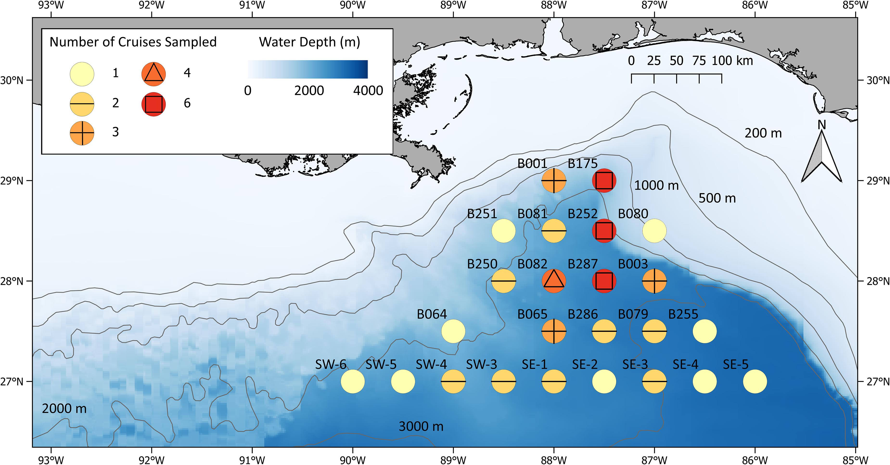
Figure 2. DEEPEND MOC10 stations sampled between 2015 and 2018. Symbol colors represent the number of cruises during which each location was sampled.
Hybrid Coordinate Ocean Model
Hybrid Coordinate Ocean Model (HYCOM), implemented at 1/25° horizontal-resolution for the GoM (18 to 31° N., 77 to 98° W.), was run in “real-time” in the weeks before and during the DEEPEND cruises (DP01 through DP06, Supplementary Table 3), providing surface and sub-surface predictions through the pelagic ocean. In order to sample important features, pre-determined cruise tracks and stations were adjusted depending on proximity to these predicted mesoscale oceanographic features (e.g., eddies and fronts). Model predictions were delivered in the form of “first-look” visualizations via web portals. The model was configured with a 32-layer hybrid (σ/z/ρ) time-variant vertical structure, which was post-processed into a time-invariant, 50-level, z-vertical structure for end-user dissemination. In this configuration, the model assimilated daily observations using 3-D variational data-assimilation, received (initial) boundary information from the Global Ocean Forecasting System (Metzger et al., 2014), and was forced by 3-h momentum and heat fluxes from the Navy Global Environmental Model (NAVGEM). Tidal boundary conditions for water level and barotropic velocity were provided by the global Ocean Tide Inverse Solution (OTIS), and rivers were implemented as a “precipitation bogus,” specified by a monthly climatological database. Further information and detailed documentation about HYCOM can be found at hycom.org.
For the DEEPEND cruise campaigns, the model provided up to 120 h of forecasts, at 3-h frequency, of the 3-D oceanic physical environment (sea surface height, ocean currents, temperature, and salinity). The HYCOM model was initialized on January 1, 2015 and ran continuously through December 31, 2018. Its outputs for 2015 (Cruises DP01 and DP02), 2016 (DP03 and DP04), 2017 (DP05), and 2018 (DP06) were deposited in the Gulf of Mexico Research Initiative Information and Data Cooperative (GRIIDC; Supplementary Table 5).
Remote Sensing/Chlorophyll
In the GoM, the location and intensity of mesoscale features can change dramatically in a few days, requiring that ocean color imagery be used to determine the precise location of surface features (e.g., Figure 3), especially the location of Mississippi River plumes and the Loop Current. While the location of surface fronts may not coincide with water mass boundaries at bathypelagic depths, the material and energetic relationships between euphotic and deeper waters were considerations when planning DEEPEND sampling transects.
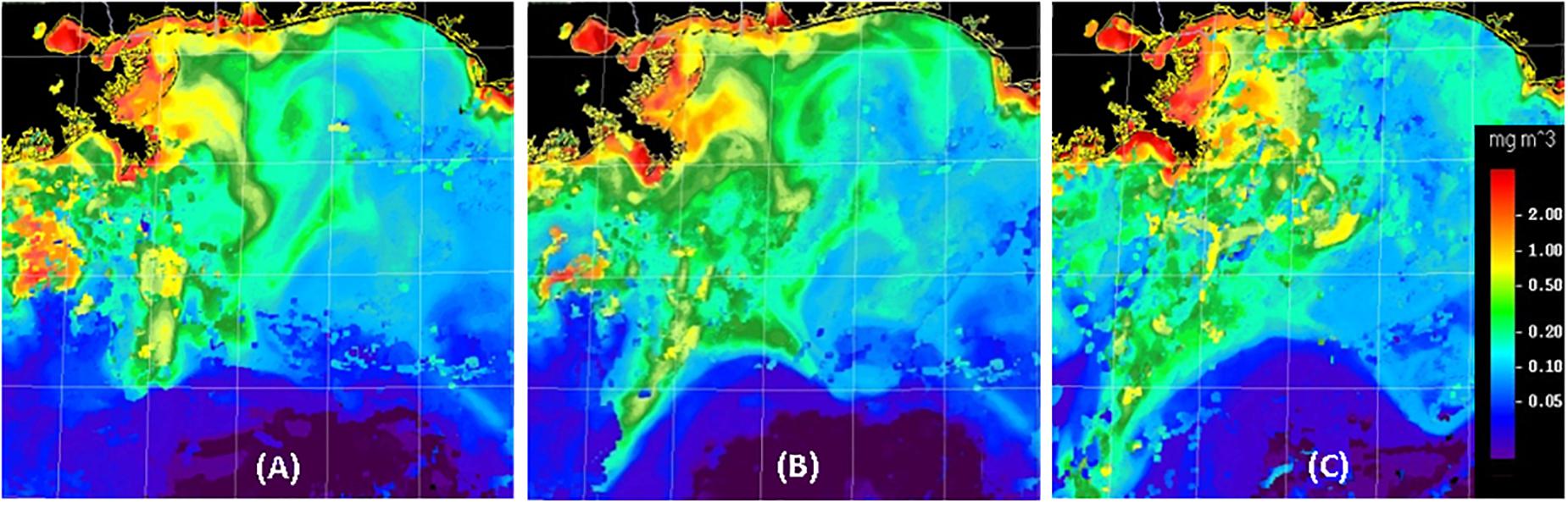
Figure 3. Examples of MODIS ocean-color composite images created for the DEEPEND study region (26–30°N, 85–91°W) during DP06 (A–C for July 22, 25, and 30, 2018, respectively). Imagery from several days was combined to emphasize recent surface feature locations. In agreement with HYCOM model predictions, features in the left portion of these images tended to move toward the southwest at more than 20 km per day, while features in the lower central portion of the images were influenced by the Loop Current and moved to the east-southeast at about 50 km per day.
Ocean color satellite images from the Moderate Resolution Imaging Spectroradiometer (MODIS) satellite were processed at the University of South Florida (USF) Optical Oceanography Laboratory through a Virtual Antenna System (VAS; Hu et al., 2013). Ocean color imagery is based on spectral reflectance of the surface ocean, which depends on the absorption and scattering of sunlight in near surface waters and therefore carries information on surface water constituents such as phytoplankton chlorophyll and colored dissolved organic matter (CDOM). The chlorophyll imagery was derived using NASA standard algorithms to remove atmospheric effects and convert surface reflectance to chlorophyll (Hu et al., 2012). Clouds, sunlight, and limited viewing angles can reduce the area of reliable ocean color satellite data. Thus, multi-day composites of MODIS ocean color imagery were created to decrease the fraction of the cruise area imagery that would otherwise have been masked or obscured. Due to the movement of surface fronts (sometimes more than 20 km over several days; Figure 3), satellite images from several days (up to a week) were combined such that the locations of ocean color features in the most recent images would be emphasized. The composites were sent to the Chief Scientist aboard the ship and the supervisor of glider operations so that transects could be adjusted to avoid or examine particular features. While sea surface temperature (SST) imagery was also examined, solar heating of the surface waters diminished the practical use of SST imagery to monitor the changing location of mesoscale features during the late-season (August) cruises.
Field Sampling and Water-Column Sensing
Net Sampling
The vertical distribution of micronekton in the water column from the surface to 1,500 m was quantified by sampling discrete-depth intervals using a Multiple Opening Closing Net and Environmental Sensing System (Wiebe et al., 1985; Sutton et al., 2010) with an effective mouth area of 10 m2 (referred to as MOC10 hereafter; Figure 4) when towed at a 45o angle. The MOC10 (3.41 × 4.69 m mouth opening) was equipped with six nets of 3-mm uniform mesh which were opened and closed at specific depth intervals on command from the ship through conducting trawl wire. This procedure yielded one oblique sample from the surface to the maximum depth sampled (net 0) and five discrete-depth samples (nets 1–5, Table 1). The rationale for these depth intervals, following Sutton (2013) and listed from deep to shallow, was: Net (1) sample the bathypelagic fauna living below the deep hydrocarbon/dispersant plume [i.e., below 1,200 m depth; Net (2)] sample the bathypelagic fauna within the stratum occupied by the deep plume (1,000 to 1,200 m depth); Net (3) sample the deep mesopelagic fauna (600 to 1,000 m, the daytime depths of occurrence of most vertically migrating taxa and persistent depth of occurrence of non-migrating mesopelagic taxa); Net (4) sample the fauna within the upper mesopelagic zone (200–600 m, daytime depths of shallow mesopelagic migrators and nighttime depth of weakly migrating taxa); and Net (5) sample the fauna of the epipelagic zone (0–200 m, the nighttime depths of most vertically migrating mesopelagic taxa and persistent depth of non-migrating surface fauna). Trawling was conducted twice at each station, centered at solar noon and midnight, to quantify diel vertical migration. Instruments were mounted to the trawl frame to measure depth, temperature, and salinity [conductivity], as well as the mouth angle of the net through the water. The volume of water filtered by each MOC10 net was measured by a Tsurumi-Sikie-Kosakusho Co., Ltd. flowmeter mounted on the MOC10 frame (adjusted for towing angle) facing directly into the flow of water. The trawl was towed at 1.5–2.5 knots and retrieved at a rate of 5 m min–1. The total volume of water filtered varied by net depth stratum and ranged from 6,500 to 70,000 m3 (Supplementary Tables 1,3). During the ONSAP, MOC10 sampling on the M/V Meg Skansi occurred almost continuously from January to September 2011 (Figure 1). In total, 241 trawl deployments were conducted at 58 stations, yielding 936 quantitative, discrete-depth samples (Supplementary Table 1). During DEEPEND, sampling occurred in either May or August (the height of dry and wet seasons in the GoM, respectively) aboard the R/V Point Sur from 2015–2018 (Figure 2). In total, 122 trawl deployments were conducted at 24 stations, yielding 470 quantitative, discrete-depth samples (Supplementary Table 3). A quantitative sample was defined as having been collected within the depth bins detailed in Table 1 as well as having a valid measurement of the volume of seawater filtered by that net.
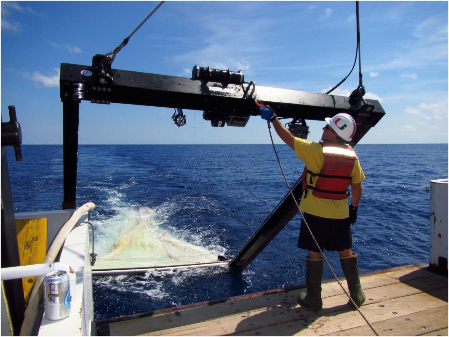
Figure 4. MOC10 unit used to quantitatively sample discrete-depth strata during ONSAP and DEEPEND cruises. Image courtesy of DEEPEND/Danté Fenolio. Written informed consent was obtained from the individual for the publication of any potentially identifiable images included in this article.
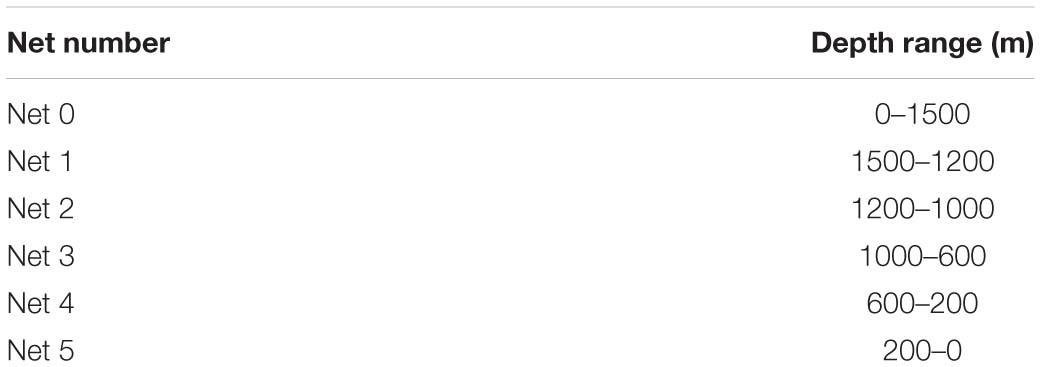
Table 1. Discrete-depth ranges targeted for sampling via MOC10 during both ONSAP and DEEPEND cruises.
The MOC10 system was chosen for its discrete-depth sampling capability (versus non-closing nets), a key consideration for quantifying the abundance of vertically migrating taxa. The 10 m2 MOCNESS was chosen over a 1 m2 MOCNESS, as the former selects for micronekton (2–20 cm body length) as opposed to plankton (Wiebe and Benfield, 2003). The fixed mouth area and the integrated flow meter allow for precise quantitative sampling, a prerequisite for time-series analysis. Lastly, the MOC10 can be deployed from an intermediate (regional-class) research size vessel with a single aft winch and conducting cable. Larger, dual-warp trawls require larger, fisheries-capable research vessels whose expense and availability are often prohibitive. That said, there are caveats with any sampling system, including the MOC10. The mouth and mesh size of rectangular midwater trawls limit the speed at which they can be towed, allowing for net avoidance by larger, more mobile taxa (Pearcy, 1983; Kaartvedt et al., 2012; Kwong et al., 2018). The multiple opening/closing nets may also be prone to “net contamination,” where animals from non-target strata can squeeze through the mouth bars of a closed net. We found the latter to be infrequent, and readily recognizable when it occurred. Taking all these factors into consideration, the MOC10 was determined to be the best gear to sample deep-pelagic micronekton/nekton in the GoM in a quantitative fashion in order to accomplish the goals of ONSAP and DEEPEND.
Midwater Trawl Sample Processing
ONSAP
After each MOC10 deployment and retrieval, individual nets were washed down with seawater and the contents of each codend were rinsed into separate numbered containers. Specimens from each codend sample were then concentrated with a sieve and placed into labeled collection jars and preserved. Larger specimens were curated separately in labeled jars. Nets 1–5 were preserved with buffered 10% formalin: seawater, while net 0’s were preserved in 95% non-denatured ethanol (EtOH) for genetic analyses. When the size or amount of gelatinous zooplankton exceeded storage capacity, individuals of each taxon were sorted into a graduated beaker, the volume and weight recorded, and the animals discarded at sea. The remaining gelatinous individuals were preserved with the rest of the catch. No sub-sampling occurred during at-sea processing. After each cruise, the samples were transported to Nova Southeastern University’s (NSU) Oceanic Ecology Laboratory, where they were sorted by major taxon, and distributed to the appropriate laboratory for species-level identifications by experts within each major taxonomic group. Specimens were then enumerated, weighed, and measured. Data were entered and stored as described in section “Biotic databases.”
DEEPEND
Midwater trawl sample processing at sea was more involved during DEEPEND than ONSAP (i.e., there was extensive subsampling for genetic and biogeochemical analyses), requiring additional handling and data management procedures. Upon retrieval of the MOC10, catches from each net were rinsed into separate containers and kept in cold (4°C) seawater during shipboard processing. This step is extremely important; deep-pelagic animals tend to degrade quickly at room temperature due to their chemical composition. Samples were sorted separately and sequentially to avoid mixing specimens from different collection nets (i.e., depth strata). While each sample was being processed, all others were stored in a refrigerator at 4°C.
Fishes, crustaceans, and cephalopods were rough-sorted by higher taxon and then identified to lower taxonomic levels (usually species) by onboard taxonomic specialists. Identified animals were counted and weighed to the nearest gram on a motion-compensating scale in batches per lowest taxonomic unit. Up to 25 specimens of each taxonomic unit were measured to the nearest millimeter per sample. All data were entered directly into the DEEPEND Nekton Database at sea (see section “Biotic databases” for biotic database description). Animals that were not subsampled for other analyses (described below) were preserved and brought back to the lab. Animals that were not identified to species at sea were examined in the lab post-cruise for further identification.
Genetics sub-sampling
As part of DEEPEND’s initiative to catalog the species diversity of the deep-pelagic waters of the GoM, a ∼650 bp segment of the mitochondrial Cytochrome c oxidase I (COI) gene and/or a ∼550 bp segment of the large mitochondrial subunit 16 or 28S genes were sequenced from a subset of fishes, crustaceans, and cephalopod species. This method, “DNA barcoding,” allows researchers to use a partial DNA sequence to identify an organism to the species level. It is particularly helpful in cases where the specimen represents an undescribed, “cryptic” species, an undescribed early-life-history form, or when definitive morphological characters are not available (e.g., male anglerfishes, trawl-damaged specimens, etc.).
Tissue samples for genetic barcoding were taken from up to 10 specimens of each fish species and up to five specimens of each crustacean and cephalopod species collected during DEEPEND cruises. Initial morphological identifications were conducted at sea, and subsequently checked by COI, 16S, and/or 28S barcoding (depending on taxonomic group). Tissues were preserved in either 95% non-denatured EtOH or RNALater. In addition to these samples, up to 50 tissue samples per cruise were collected for temporal population genomics studies (ddRADseq; Peterson et al., 2012) of eight fish species and six crustacean species (Timm et al., 2020b, Supplementary Table 6). Additionally, tissue samples from three species of cephalopods were used to compare the genetic connectivity of each species between the GoM (Supplementary Table 6) and the Bear Seamount region of the northern Atlantic Ocean (Timm et al., 2020a). In all cases, paired plastic identification tags were kept with each tissue sample and the corresponding individual voucher specimen to maintain data integrity before, during, and after barcoding procedures.
These methods have proven useful for the study of diversity, health and resilience in the GoM (Judkins et al., 2016, 2020; Timm et al., 2019, 2020a,b). A major challenge of the DNA barcoding method was matching the genetic sequences with those already submitted by other researchers in the Barcode of Life Database. There were many instances where either one genetic sequence had more than one species name assigned to it, multiple sequences were attributed to the same species, or the species name listed in the database conflicted with the identification made by DEEPEND taxonomic experts.
Stable isotope analysis sub-sampling
A thorough understanding of deep-pelagic ecosystems requires detailed knowledge of food webs including descriptions of feeding relationships among taxa, estimations of trophic position, and delineations of energy flow. Food webs have traditionally been examined through gut content analysis (GCA) which can require thousands of samples, a high level of taxonomic expertise, and is best suited for organisms that ingest prey whole. SIA is a powerful complement to GCA, as it is not as dependent on taxonomic expertise, can be applied to a range of taxa regardless of feeding mode, and can be conducted with fewer samples. However, interpretation of SIA data can be difficult due to significant spatiotemporal variation in the isotopic signatures of primary producers (isotopic baseline) which can be conserved in higher-order consumers resulting in misinterpretation of feeding relationships and incorrect trophic position estimates. Amino acid compound-specific isotope analysis (AA-CSIA) is a more refined technique that can help distinguish between variation in consumer isotopic signatures caused by changes in the isotopic baseline and changes in the diets and feeding habits of consumers (Popp et al., 2007). The method uses “source” amino acids that accurately reflect the isotope values of primary producers and “trophic” amino acids that can be used as indicators of change in consumer feeding and diet (McClelland and Montoya, 2002; Chikaraishi et al., 2009). Given the advantages of SIA, and because several high quality GCA datasets currently exist for deep-pelagic assemblages in the GoM (Flock and Hopkins, 1992; Hopkins et al., 1996), SIA and AA-CSIA were employed to provide a complementary description of the trophic structure of deep-pelagic assemblages in the GoM (Richards et al., 2019, 2020). To better inform the study design, catch data from MOC10 sampling and prior GCA investigations in the GoM were leveraged to identify numerically dominant species that represent important energy vectors connecting primary and secondary production with higher-order consumers. These species encompassed an array of migratory strategies (synchronous vertical migrators, asynchronous vertical migrators, and non-migrators) and feeding modes (Supplementary Table 6). Additionally, data from the HYCOM and MODIS were used to ensure specimens were collected from salient mesoscale features (e.g., cyclonic and anticyclonic eddies, Mississippi River plume), providing as complete a representation of deep-pelagic trophic structure as possible.
Following collection through MOC10 sampling, specimens for SIA and AA-CSIA were identified and enumerated at sea, with specimens selected for bulk SIA frozen whole at −20°C, while specimens selected for AA-CSIA were frozen whole in liquid nitrogen before transport to Texas A&M University at Galveston. SIA and AA-CSIA specimens were kept in long-term storage at −20 and −80°C, respectively. Muscle tissue used for SIA and AA-CSIA was dissected from the lateral musculature of fishes, from the anterior portion of the mantle from cephalopods, and from the dorsal portion of the abdomen in decapod crustaceans. Samples were then rinsed with deionized water to remove trace carbonates, freeze dried, and homogenized using mortar and pestle. Information on remaining procedures during SIA and AA-CSIA can be found in Richards et al. (2019) and Richards et al. (2020).
Polycyclic aromatic hydrocarbon analysis sub-sampling
Polycyclic aromatic hydrocarbon (PAH) analyses were conducted on GoM deep-pelagic micronekton to determine the extent and persistence of DWHOS-derived oil contamination. Smaller fishes (<15 mm), cephalopods, and shrimp samples collected for PAH analysis were stored whole in pre-combusted (450°C for 4 h) glass vials and frozen in a −20°C freezer. The larger fishes (>15 mm) were dissected at sea to remove internal organs (liver, stomach, heart, and intestines), gills, muscle tissue, and eggs (if present). Each dissected tissue was stored separately and frozen. All samples were transported on dry ice to USF (Supplementary Table 6). Whole-body samples were dissected at USF to collect internal organs, muscle tissue, and eggs (if present) from fishes and shrimps, and mantle tissue and eggs (if present) from cephalopods. For a complete description of methods and findings for fishes see Romero et al. (2018) and for cephalopods see Romero et al. (2020).
In situ Sensing
Abiotic Sensing
MOC10 sensors
The MOC10 was outfitted with pressure (depth), temperature, and conductivity (salinity) sensors, which were calibrated annually. The sensors recorded a reading once every four seconds during the entire tow.
CTD sensors
ONSAP
A Sea-Bird SBE 19 plus V2 CTD profiling package was deployed at each station to at least 1,500 m (when the bottom depth was greater than 1600 m). Stations with water depths less than 1,600 m were profiled to full water column depth within 100 m of the bottom (Supplementary Table 2). The CTD was mounted to a 12-Niskin bottle (12-L) rosette and equipped with a dissolved oxygen sensor (Sea-Bird SBE-43), two fluorometers (WET Labs CDOM and WET Labs ECO-AFL/FL), and a turbidity meter (WET Labs ECO-NTU). The CTD data were processed following the DWH-NRDA CTD processing protocol. Calibrated data from each sensor were averaged in 1-m bins within Sea-Bird’s SBE Processing software. For all deployments, only data from the downcasts were used in characterizing the water column structure.
DEEPEND
A 12-Niskin bottle (12-L) rosette with CTD was deployed from the R/V Point Sur at DEEPEND stations (Figure 2), usually to depths greater than 1,000 m. There were 106 CTD profiles collected during the DEEPEND cruises (Supplementary Table 4). The Sea-Bird 911plus CTD on the sampling rosette combined measurements of conductivity, temperature, and pressure, with additional sensors connected to the CTD on a per-cruise basis. These sensors included one or more dissolved oxygen sensors (Sea-Bird SBE-43), a transmissometer (WET Labs C-Star), and fluorometers (WET Labs ECO CDOM, ECO chlorophyll a, or Chelsea UV Aquatracka). The number and type of sensors varied between cruises, but information from the dissolved oxygen sensor and chlorophyll fluorometer was available at almost all of the DEEPEND stations. The CTD data were post-processed using Sea-Bird’s SBE Data Processing software, which converted the data to engineering units as well as computed salinity and dissolved oxygen concentrations. To increase the consistency of in situ chlorophyll a fluorometer results between the DEEPEND cruises, the measurements of water-sample chlorophyll a and CDOM absorbance were used to scale the CTD’s in situ fluorometer measurements. The measurements were binned (using median values) into 1-m depth intervals. Both the raw and binned CTD data for each DEEPEND cruise are available through the GRIIDC data repository (Supplementary Table 5).
Slocum glider sensing
During select DEEPEND cruises, a 1000-m depth-rated Slocum Electric Glider (Figure 5) was used to characterize the upper 400 m (on average) of the GoM water column. The glider was equipped with a Seabird SBE41CP CTD, two WET Labs fluorometers, two Satlantic radiometers, and an Aanderaa dissolved oxygen sensor. The fluorometers were equipped to sample for chlorophyll, CDOM, backscatter at 660 and 880 nm, and turbidity. All sensors sampled at 0.25 Hz. The radiance and irradiance sensors sampled at four wavelengths: ∼412, 443, 556, and 683 nm. The glider transited vertically between 2 m and max depth (ranging from 400–800 m) at ∼0.1 m/s which resulted in a vertical sample resolution of ∼0.4 m. The measurements were taken at various depths and included conductivity, temperature, depth, chlorophyll fluorescence, gelbstoff fluorescence, dissolved oxygen, and light field measurements. While the glider was deployed at sea, it surfaced and communicated to an onshore control station at predetermined intervals, typically every 3 h. Launch, transit progress, and recovery of the glider position were planned and conducted, in part, by utilizing the HYCOM to provide context of the predicted current structure of the Loop Current and eddies. Model input for mission planning allowed glider adaptive sampling of features and assisted piloting to avoid unfavorable currents wherever possible. Once recovered, the complete measurement suite was downloaded from the vehicle, processed, and made available through USF and national data archives, including GRIIDC. The glider temperature and salinity data were assimilated into the HYCOM to assist in analyses of subsurface water characteristics and validation of ocean models, which was used to support the DEEPEND cruises.
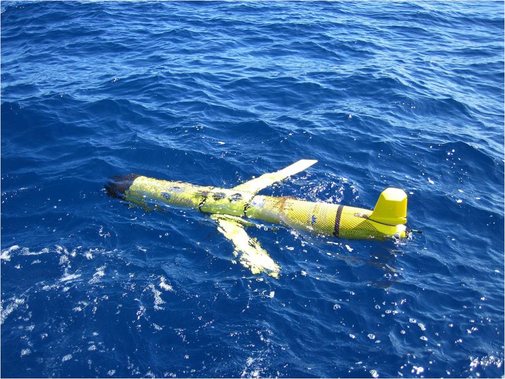
Figure 5. Slocum glider during DP02 cruise deployment.
Biotic Sensing
Acoustic backscatter
Two different vessels collected hydroacoustic data during the ONSAP and DEEPEND sampling programs. Simrad split-beam echosounder systems (EK60 and EK80) were used on both vessels; however, the transmitted frequencies varied according to vessel (Table 2). Transducers were mounted from a pole mount on both the M/V Meg Skansi and R/V Point Sur. While both vessels transmitted at 18 and 38 kHz, the higher frequencies were intermittently available. During each survey, the echosounder system was calibrated following the standard sphere method described by Demer et al. (2015). Measured gains and offsets derived from the Simrad lobe calibration program were recorded and input into the data analysis process. The echosounders were operated consistently among the surveys to ensure comparability over time. Multifrequency backscatter data were recorded simultaneously from each transceiver with a ping rate set to 0.2 Hz.

Table 2. Echosounder system properties used during multi-vessel studies in the GoM.
Analyses of raw backscatter data were processed in Echoview (PTY. Ltd.). Data were manually scrutinized for interference, noise, and other artifacts, and data processing routines were applied to reduce the effects of these on the processed data following methods outlined in D’Elia et al. (2016). Specifically, data were corrected for the effects of attenuation due to propagation losses and absorption. Intermittent noise spikes and transient noise were removed with Echoview (Ryan et al., 2015). Following that, a background noise removal process was applied (De Robertis and Higginbottom, 2007). Data were re-sampled at 500 m × 5 m (horizontal by vertical) elementary distance sampling units (EDSU) to generate analysis cells in which the echo integral was derived for each transect. Multifrequency comparisons were drawn to examine water-column backscatter between 18 and 38 kHz (D’Elia et al., 2016; Boswell et al., 2020).
The main limitation or bias associated with this method is attributing the backscatter to specific taxa. Using “ground-truth” data from direct biological sampling (i.e., nets) to interpret the backscatter patterns is the ideal methodology and was employed in both ONSAP and DEEPEND. Another potential limitation when using acoustic data across wide depth ranges is the potential effect of resonance when vertically migrating animals with gas bladders change depth. This effect occurs because backscattering intensity changes as a function of the surface area of a gas bladder. Therefore, it is important to interpret acoustic data carefully to account for this possibility (Davison et al., 2015; Proud et al., 2019).
Water Sampling
During DEEPEND cruises, CTD profiles were used to identify the depths of four “features of interest” at each station where water samples were collected. The features of interest included the surface layer, the chlorophyll-maximum layer, the oxygen-minimum zone, and the maximum trawl depth at each station. The depths of the chlorophyll maximum and oxygen-minimum zone, which varied by station, were determined visually during the CTD downcast using real-time data collected by fluorometer and oxygen sensors. Once the station-specific water collection depths were determined, three Niskin bottles were fired at each of the four targeted depths during the CTD upcast, yielding 36 L per depth.
Optical Absorption of Particulate and Dissolved Material and Determination of Chlorophyll a Concentration
The absorption of light within the surface waters is a dominant factor in determining ocean color. Measurements of the optical absorption spectra for particulates and dissolved material in water samples were collected because they provide information for the validation of ocean color imagery (e.g., section “Remote sensing/chlorophyll”), information about the pigment composition of phytoplankton in a water sample, and a measurement of the concentration of chlorophyll and dissolved material in that water sample. Samples from waters near the sea surface (<5 m depth) and the chlorophyll maximum were used not only to estimate the chlorophyll a concentration, but also to separate the water’s optical absorption spectra into contributions from the sample’s particulate material, ap(λ), detrital material, ad(λ), and CDOM, aCDOM(λ). Shortly after collection, samples were filtered through a glass fiber filter to separate the particulate constituents from a water sample, with additional filtration to partition the dissolved material. Both the filter pad and filtrate were then stored for additional processing and analysis ashore.
The chlorophyll a and CDOM measurements from the water samples were used to standardize the in situ fluorometry values as mentioned in section “DEEPEND”. While the variability in the relationship between in situ fluorometric measurements and chlorophyll a concentrations and the necessity of validation measurements is often acknowledged, the normalization of the fluorometric data is frequently omitted in presentations of the in situ fluorometry (Roesler et al., 2017). Not only was the in situ environment during the DEEPEND cruises different than those used for factory fluorometer calibrations, different fluorometers were used with the CTD on different cruises. The optical absorption information from the filter pads was used to improve the consistency of in situ fluorometric measurements between different casts and cruises.
The determination of optical absorption using this filter pad method requires several liters of sample water for the clear waters found throughout much of the DEEPEND sampling region. This relatively large volume of sample water, and the time and effort needed to filter and process that water, limits the number of water sampling depths that can be practically collected from a CTD cast. Though the samples were intended to capture representative waters from CTD profile features (e.g., chlorophyll maximum depth intervals), unsampled variations in planktonic composition and optical properties may occur within features. Chlorophyll a concentration and optical absorption spectra data are available through the GRIIDC data repository (Supplementary Table 5).
Microbial Community Characterization
Seawater microbial sampling followed routine methods, as described in Easson and Lopez (2019), to capture the dynamics of microbial plankton communities in relation to a host of biotic and abiotic factors. Briefly, seawater samples from all four targeted depths (surface, chlorophyll maximum, oxygen minimum, and maximum depth) were passed through 0.45-um hydrophilic mixed cellulose ester filters, which were then frozen and stored at −20°C for subsequent DNA extractions post-cruise. Subsequent next-generation sequencing and microbial community analyses were conducted following the methods of Easson and Lopez (2019). During seawater collection, environmental metadata were simultaneously collected with instruments on the CTD. These metadata provided context for determining function and structure of the subsequently described microbial communities.
The two main limitations of this method are that it does not directly identify the function of community members or provide an absolute abundance estimation (only relative abundance). Assumptions are made based on substantial literature evidence that these communities are responding directly to a particular influence. Despite these limitations, these data remain useful in capturing how microbial plankton dynamics are related to several biological and oceanographic variables.
Stable Isotope Analysis of Particulate Organic Matter
Because a consumer’s isotopic signature is determined by both its position in the food web and the isotope value of primary producers, isotopic variation in primary producers can lead to isotopic variation in consumers not reflective of a change in diet or trophic status. Thus, when conducting SIA it is essential to characterize the isotopic signatures of relevant primary producers so that variation in consumer isotope values caused by shifting isotope values in primary producers can be distinguished from changes caused by differences in the feeding habits of consumers. In order to establish an isotopic baseline in the pelagic GoM, we conducted SIA on samples of particulate organic matter (POM) to serve as a proxy for phytoplankton primary production in the region. Water samples for POM were initially collected from 12-L Niskin bottles deployed during CTD casts and then transferred to clean 1-L Nalgene bottles, which were inverted into 500-ml Pall magnetic filter funnels. Samples of POM were then obtained by filtering 5 – 20 L of water through pre-combusted (2 h at 450°C) 47-mm (surface and chlorophyll maximum) and 25-mm (oxygen minimum and maximum trawl depth) glass microfiber filters (GF/F) under low pressure. Once sufficient material had been obtained, filters were stored frozen at −20°C until processing for SIA.
Collections and Databases
Specimen Collections
The majority of specimens (fishes, crustaceans, and gelatinous zooplankton) collected during both ONSAP and DEEPEND are housed at the Guy Harvey Oceanographic Center, Nova Southeastern University, Dania Beach, FL and tracked through the biotic databases described in section “Biotic databases.” Molluscan specimens were deposited in the National Museum of Natural History, Washington, DC, United States, or at the USF St. Petersburg, St. Petersburg, FL, United States. All crustacean specimens used for genetics, including tissue and DNA extracts, were assigned catalog numbers (HBG#) in curated, databased research collections. All voucher specimens and tissues were archived in the Florida International Crustacean Collection (FICC), which currently houses over ∼10,000 curated crustacean specimens.
The holotypes and paratypes for new species discovered during these projects (e.g., Pietsch and Sutton, 2015; Judkins et al., 2020) were deposited in museum collections appropriate for each taxonomic group. Crustaceans and cephalopods were deposited at the National Museum of Natural History, Washington, DC, United States. Fishes will be deposited in one of several museums based on the specific taxon: Lophiiformes will be deposited at the Burke Museum, University of Washington, Seattle, WA, United States; Stomiiformes will be deposited at the Museum of Comparative Zoology, Harvard University, Cambridge, MA, United States; and representative subsets of the entire collection, or select specimens, will be deposited at the Scripps Institution of Oceanography, the Louisiana State University Ichthyology Collection, the Tulane Ichthyology Collection, the Virginia Institute of Marine Science Ichthyology Collection, the Yale Peabody Museum of Natural History, and the Florida Museum of Natural History.
Biotic Databases
All biotic data are stored in Microsoft Access databases at the Oceanic Ecology Laboratory at NSU (T. Sutton). Data collected during the ONSAP are stored as “Nekton_Database_DDMMYY.accdb” and data collected during DEEPEND are stored as “DEEPEND_Nekton_Database_DDMMYY.accdb.” These are relational databases stored on NSU’s servers with replication. There are three main tables: (1) Field Sample/Trawl Field Data table containing the station and sampling depth information, (2) Nekton Database table containing the catch information (taxon, catch in numbers, weight, etc.), and (3) Taxon List table containing the hierarchical taxonomic information (class, order, family, etc.).
In addition, there are other tables to look up and combine data. A Primary Key connects these tables to one another.
Database Availability
DIVER
Biotic and abiotic data collected during the ONSAP are publicly available through NOAA’s Data Integration Visualization Exploration and Reporting (DIVER) tool found at https://www.diver.orr.noaa.gov/. DIVER is a data warehouse and query tool that allows public access to NOAA’s Damage Assessment, Remediation, and Restoration Program data. These data are collected in response to, and/or restoration of, environmental damage caused by oils spills, releases of hazardous waste, or vessel groundings. The DIVER Explorer query tool can be used to search, filter, and download these data using links to popular datasets, guided queries, or keyword searches. Data mentioned in this paper can be located by linking to the popular dataset “Deepwater Horizon NRDA data” and performing a keyword search for “Meg Skansi.”
GRIIDC
Biotic (ONSAP and DEEPEND) and abiotic (DEEPEND only) data are also publicly available through the GRIIDC, housed at the Harte Research Institute for GoM Studies at Texas A&M University, Corpus Christi. GRIIDC is a team of researchers, data and topic specialists, and information technology professionals who have developed a data management system to organize, store, and disseminate data collected by GoM researchers as part of the Master Research Agreement between British Petroleum (BP) and the GoM Alliance. GRIIDC has secured a funding agreement with the GoMRI, the funding body of the GoM Alliance, to continue providing data management and the dissemination of datasets to the scientific community (both GoMRI funded and non-GoMRI funded research) for a minimum of 10 years beyond the conclusion of formal GoMRI funding in 2020 (i.e., through the year 2030, at a minimum).
All data produced by GoMRI-funded individuals and research consortia (such as DEEPEND) are required to be submitted to the GRIIDC repository in a timely fashion, typically within one year of data collection and/or processing. Upon submission, all datasets undergo a rigorous vetting process led by GRIIDC subject matter experts who work with researchers and the Data Manager to ensure data integrity, organization, and discovery, including descriptive, ISO-19115-2 compliant metadata. All datasets housed by GRIIDC are assigned Digital Object Identifiers (DOIs) in the same manner as publications to allow future researchers to use and cite the data. See Supplementary Table 5 for a list of datasets and their corresponding DOIs. All datasets are available at https://data.gulfresearchinitiative.org/.
NCEI
Most environmental data, such as CTD and ship along-track measurements, were submitted on behalf of DEEPEND to the National Centers for Environmental Information (NCEI) through a proprietary process developed between NCEI and GRIIDC. Calibrated water column acoustic backscatter data, including associated metadata, collected during the DEEPEND program are also archived at NCEI. The archive includes raw acoustic backscatter data for each station that has corresponding net tow data (Supplementary Table 5).
NCBI
DNA sequences obtained from barcoding were submitted on behalf of DEEPEND to the National Center for Biotechnology Information (NCBI) database. A compendium of specimen information that includes ID Number, Cruise Number, Collection Date, Collection Location, Taxonomic Species Identity (Order, Family, Genus, and Species), and NCBI GenBank Accession Numbers have been deposited into GRIIDC (Supplementary Table 5). Additionally, the small subunit rRNA gene was sequenced from samples collected in the water column to identify the microbial community. These sequences were deposited in the NCBI Short Read Archive where bioproject accession numbers were assigned.
Data Availability Statement
Data are publicly available through the Gulf of Mexico Research Initiative Information & Data Cooperative (GRIIDC) at https://data.gulfresearchinitiative.org (doi: 10.7266/N7R49P43; 10.7266/N7MC8XDC; 10.7266/n7-ceq1-5g82; 10.7266/N7GM85P1; 10.7266/N73R0QSX; 10.7266/N7PV6HS1; 10.7266/N7Q52N08; 10.7266/N7KD1W8J; 10.7266/N7VM49MP; 10.7266/N7QR4VK0; 10.7266/N7X065FZ; 10.7266/N70K26W5; 10.7266/n7-77gs-w736; 10.7266/N7FF3QFK; 10.7266/N7610XD5; 10.7266/N72805Q8; 10.7266/N7XG9P7F; 10.7266/N7JD4V45; 10.7266/n7-j3c9-4s47; 10.7266/N7TM78J6; 10.7266/N7ZC818X; 10.7266/N7NC5ZK6; 10.7266/N7ZK5F24; 10.7266/n7-bhzk-nh73; 10.7266/N7CN729W; 10.7266/N7H41PX6; 10.7266/N7474871; 10.7266/N76T0K11; 10.7266/N7BK19RB; 10.7266/n7-ac8e-0240; 10.7266/N70P0X3T; 10.7266/N7VX0DK2; 10.7266/N7XP7385; 10.7266/N7902234; 10.7266/n7-dd3p-t155; 10.7266/n7-05f6-th15; 10.7266/N7ZG6QQ9; 10.7266/N7XP73B2; 10.7266/N7HM56TD; 10.7266/N71C1TZC; 10.7266/n7-1xs7-4n30; 10.7266/n7-3p3y-g470; 10.7266/n7-hhnq-kh83; 10.7266/N75M63Q3; 10.7266/n7-c56k-dp86; 10.7266/N7VX0F19; 10.7266/n7-9yq3-3177; 10.7266/n7-rg4t-2k74; 10.7266/n7-67wg-mz19; 10.7266/n7-ws46-0612; 10.7266/n7-rmfn-4d68; 10.7266/N7GF0RW0; 10.7266/N7Z036HF; 10.7266/n7-k9tp-y248; 10.7266/n7-033n-s709; 10.7266/n7-awwx-4g13; 10.7266/N79K48MZ; 10.7266/N7P55KWX; 10.7266/N7833QCP; 10.7266/N7XD1026; 10.7266/N7QZ28B4; 10.7266/n7-jxss-1s14; 10.7266/n7-bf8a-hq12; 10.7266/n7-bzef-0e24; 10.7266/N7ZS2V04; 10.7266/N75D8Q7Z; 10.7266/n7-3t9h-8p38; 10.7266/N7319T92; 10.7266/N7ZP44GF; 10.7266/N73B5XHK; 10.7266/N7TX3CQ8; and 10.7266/N70Z71NN).
Ethics Statement
The animal study was reviewed and approved by the Florida Atlantic University Institutional Animal Care and Use Committee.
Author Contributions
All authors conducted the research, analyzed the data, and contributed to the manuscript. AC and TS oversaw all aspects of this research, including specimen, sample, and data collection, analysis and data management. All authors have agreed to being listed as such and approve of the submitted version of this manuscript.
Funding
This research was funded in part by the NOAA Office of Response and Restoration and in part by a grant from The Gulf of Mexico Research Initiative (GoMRI).
Conflict of Interest
The authors declare that the research was conducted in the absence of any commercial or financial relationships that could be construed as a potential conflict of interest.
Acknowledgments
We thank the captains and crews of the M/V Meg Skansi and R/V Point Sur for their excellent shipboard services. We are thankful for the shore-based support from Continental Shelf Associates, particularly Gray Lawson and Eddie Hughes, and from the Louisiana Universities Marine Consortium. We thank Okeanus Science and Technology and Sea-Gear Corporation for equipment support. Our sincerest thanks to all of the students, laboratory techs, and research scientists who have helped collect and process an enormous sample set. This is contribution #230 from the Center for Coastal Oceans Research in the Institute of Water and Environment at Florida International University.
Supplementary Material
The Supplementary Material for this article can be found online at: https://www.frontiersin.org/articles/10.3389/fmars.2020.548880/full#supplementary-material
References
Androulidakis, Y., Karourafalou, V., Le Hénaff, M., Kang, H. S., Sutton, T. T., Chen, S., et al. (2019). Offshore spreading of Mississippi waters: pathways and vertical structure under eddy influence. J. Geophys. Res. Oceans 124, 5952–5978. doi: 10.1029/2018JC014661
Beyer, J., Trannum, H. C., Bakke, T., Hodson, P. V., and Collier, T. K. (2016). Environmental effects of the Deepwater Horizon oil spill: a review. Mar. Poll. Bull. 110, 28–51. doi: 10.1016/j.marpolbul.2016.06.027
Boswell, K. M., D’Elia, M., Johnston, M. W., Mohan, J. A., Warren, J. D., Wells, R. J., et al. (2020). Oceanographic structure and light levels drive patterns of sound scattering layers in a low-latitude oceanic system. Front. Mar. Sci. 7:51. doi: 10.3389/fmars.2020.00051
Camilli, R., Reddy, C. M., Yoerger, D. R., Van Mooy, B. A. S., Jakuba, M. V., Kinsey, J. C., et al. (2010). Tracking hydrocarbon plume transport and biodegradation at Deepwater Horizon. Science 330, 201–204. doi: 10.1126/science.1195223
Chikaraishi, Y., Ogawa, N. O., Kashiyama, Y., Takano, Y., Suga, H., Tomitani, A., et al. (2009). Determination of aquatic food-web structure based on compound-specific nitrogen isotopic composition of amino acids. Limnol. Oceanogr.-Meth. 7, 740–750. doi: 10.4319/lom.2009.7.740
Davison, P. C., Koslow, J. A., and Kloser, R. J. (2015). Acoustic biomass estimation of mesopelagic fish: backscattering from individuals, populations, and communities. ICES J. Mar. Sci. 72, 1413–1424. doi: 10.1093/icesjms/fsv023
De Robertis, A., and Higginbottom, I. (2007). A post-processing technique to estimate the signal-to-noise ratio and remove echosounder background noise. ICES J. Mar. Sci. 64, 1282–1291. doi: 10.1093/icesjms/fsm112
D’Elia, M., Warren, J. D., Rodriguez-Pinto, I., Sutton, T. T., Cook, A., and Boswell, K. M. (2016). Diel variation in the vertical distribution of deep-water scattering layers in the Gulf of Mexico. Deep Sea Res. Part I 115, 91–102. doi: 10.1016/j.dsr.2016.05.014
Demer, D. A., Berger, L., Bernasconi, M., Bethke, E., Boswell, K., Chu, D., et al. (2015). Calibration of acoustic instruments. ICES Coop. Res. Rep. No. 326:133. doi: 10.25607/OBP-185
Easson, C. G., Boswell, K. M., Tucker, N., Warren, J. D., and Lopez, J. V. (2020). Combined eDNA and acoustic analysis reflects diel vertical migration of mixed consortia in the Gulf of Mexico. Front. Mar. Sci. 7:552. doi: 10.3389/fmars.2020.00552
Easson, C. G., and Lopez, J. V. (2019). Depth-dependent environmental drivers of microbial plankton community structure in the northern Gulf of Mexico. Front. Microbiol. 9:3175. doi: 10.3389/fmicb.2018.03175
Eldridge, P. J. (1988). The Southeast Area Monitoring and Assessment Program (SEAMAP): a state-federal-university program for collection, management, and dissemination of fishery-independent data and information in the southeastern United States. Mar. Fish. Rev. 50, 29–39.
Flock, M. E., and Hopkins, T. L. (1992). Species composition, vertical distribution, and food habits of the sergestid shrimp assemblage in the eastern Gulf of Mexico. J. Crust. Biol. 12, 210–223. doi: 10.2307/1549076
Frank, T. M., Fine, C. D., Burdett, E. A., Cook, A. B., and Sutton, T. T. (2020). The vertical and horizontal distribution of deep-sea crustaceans in the order Euphausiacea in the vicinity of the Deewater Horizon oil spill. Front. Mar. Sci. 7:99. doi: 10.3389/fmars.2020.00099
Hebert, P. D. N., Cywinska, A., Ball, S. L., and deWaard, J. R. (2003). Biological identifications through DNA barcodes. Proc. R. Soc. Lond. B 270, 313–321. doi: 10.1098/rspb.2002.2218
Hopkins, T. L., Sutton, T. T., and Lancraft, T. M. (1996). The trophic structure and predation impact of a low latitude midwater fish assemblage. Prog. Oceanogr. 38, 205–239. doi: 10.1016/s0079-6611(97)00003-7
Hu, C., Barnes, B. B., Murch, B., and Carlson, P. R. (2013). Satellite-based virtual buoy system to monitor coastal water quality. Opt. Eng. 53:051402. doi: 10.1117/1.OE.53.5.051402
Hu, C., Lee, Z., and Franz, B. (2012). Chlorophyll a algorithms for oligotrophic oceans: a novel approach based on three-band reflectance difference. J. Geophys. Res. 117:C01011. doi: 10.1029/2011JC007395
Johnston, M., Milligan, R., Easson, C., DeRada, S., Penta, B., and Sutton, T. (2019). An empirically-validated method for characterizing pelagic habitats in the Gulf of Mexico using ocean model data. Limnol. Oceanogr.-Meth. 17, 362–375. doi: 10.1002/lom3.10319
Judkins, H., Lindgren, A., Villanueva, R., Clark, K., and Vecchione, M. (2020). A description of three new bathyteuthid squid species from the North Atlantic and Gulf of Mexico. Bull. Mar. Sci. 96, 281–296. doi: 10.5343/bms.2019.0051
Judkins, H., Vecchione, M., and Rosario, K. (2016). Morphological and molecular evidence of Heteroteuthis dagamensis in the Gulf of Mexico. Bull. Mar. Sci. 92, 51–57. doi: 10.5343/bms.2015.1061
Kaartvedt, S., Staby, A., and Aksnes, D. L. (2012). Efficient trawl avoidance by mesopelagic fishes causes large underestimation of their biomass. Mar. Ecol. Prog. Ser. 456, 1–6. doi: 10.3354/meps09785
Kwong, L. E., Pakhomov, E. A., Suntsov, A. V., Seki, M. P., Brodeur, R. D., Pakhomova, L. G., et al. (2018). An intercomparison of the taxonomic and size composition of tropical macrozooplankton and micronekton collected using three sampling gears. Deep Sea Res. Part I 135, 34–45. doi: 10.1016/j.dsr.2018.03.013
Mantelatto, F. L., Terossi, M., Negri, M., Buranelli, R. C., Robles, R., Magalhães, T., et al. (2018). DNA sequence database as a tool to identify decapod crustaceans on the São Paulo coastline. Mitochondrial DNA Part A 29, 805–815. doi: 10.1080/24701394.2017.1365848
McClelland, J. W., and Montoya, J. P. (2002). Trophic relationships and the nitrogen isotopic composition of amino acids in plankton. Ecology 83, 2173–2180. doi: 10.1890/0012-9658(2002)083[2173:tratni]2.0.co;2
Meinert, C. R., Clausen-Sparks, K., Cornic, M., Sutton, T. T., and Rooker, J. R. (2020). Taxonomic richness and diversity of larval fish assemblages in the oceanic Gulf of Mexico: links to oceanographic conditions. Front. Mar. Sci. 7:579. doi: 10.3389/fmars.2020.00579
Metzger, E. J., Smedstad, O. M., Thoppil, P. G., Hurlburt, H. E., Cummings, J. A., Wallcraft, A. J., et al. (2014). US Navy operational global ocean and Arctic ice prediction systems. Oceanography 27, 32–43. doi: 10.5670/oceanog.2014.66
Milligan, R. J., and Sutton, T. T. (2020). Dispersion overrides environmental variability as a primary driver of horizontal assemblage structure of the mesopelagic fish family Myctophidae in the northern Gulf of Mexico. Front. Mar. Sci. 7:15. doi: 10.3389/fmars.2020.00015
Moore, J. A., Fenolio, D. B., Cook, A. B., and Sutton, T. T. (2020). Hiding in plain sight: elopomorph larvae are important contributors to fish biodiversity in a low-latitude oceanic ecosystem. Front. Mar. Sci. 7:169. doi: 10.3389/fmars.2020.00169
Oliver, T. H., Heard, M. S., Isaac, N. J., Roy, D. B., Procter, D., Eigenbrod, F., et al. (2015). Biodiversity and resilience of ecosystem functions. Trends Ecol. Evol. 30, 673–684.
Pearcy, W. G. (1983). Quantitative assessment of the vertical distributions of micronektonic fishes with opening/closing midwater trawls. Biol. Oceanogr. 2, 289–310.
Peterson, B. K., Weber, J. N., Kay, E. H., Fisher, H. S., and Hoekstra, H. E. (2012). Double digest RADseq: an inexpensive method for de novo SNP discovery and genotyping in model and non-model species. PLoS One 7:e37135. doi: 10.1371/journal.pone.0037135
Pietsch, T. W., and Sutton, T. T. (2015). A new species of the ceratioid anglerfish genus Lasiognathus Regan (Lophiiformes: Oneirodidae) from the northern Gulf of Mexico. Copeia 103, 429–432. doi: 10.2307/1446097
Popp, B. N., Graham, B. S., Olson, R. J., Hannides, C. C., Lott, M. J., López-Ibarra, G. A., et al. (2007). Insight into the trophic ecology of yellowfin tuna, Thunnus albacares, from compound-specific nitrogen isotope analysis of proteinaceous amino acids. Terr. Ecol. 1, 173–190. doi: 10.1016/s1936-7961(07)01012-3
Proud, R., Handegard, N. O., Kloser, R. J., Cox, M. J., and Brierley, A. S. (2019). From siphonophores to deep scattering layers: uncertainty ranges for the estimation of global mesopelagic fish biomass. ICES J. Mar. Sci. 76, 718–733. doi: 10.1093/icesjms/fsy037
Pruzinsky, N. M., Milligan, R. J., and Sutton, T. T. (2020). Pelagic habitat partitioning of late-larval and juvenile tunas in the oceanic Gulf of Mexico. Front. Mar. Sci. 7:257. doi: 10.3389/fmars.2020.00257
Richards, T. M., Gipson, E. E., Cook, A., Sutton, T. T., and Wells, R. D. (2019). Trophic ecology of meso-and bathypelagic predatory fishes in the Gulf of Mexico. ICES J. Mar. Sci. 76, 662–672. doi: 10.1093/icesjms/fsy074
Richards, T. M., Sutton, T. T., and Wells, R. D. (2020). Trophic structure and sources of variation influencing the stable isotope signatures of meso- and bathypelagic micronekton fishes. Front. Mar. Sci. 7:507992. doi: 10.3389/fmars.2020.507992
Roesler, C., Uitz, J., Claustre, H., Boss, E., Xing, X., Organelli, E., et al. (2017). Recommendations for obtaining unbiased chlorophyll estimates from in situ chlorophyll fluorometers: a global analysis of WET Labs ECO sensors. Limnol. Oceanogr.-Meth. 15, 572–585. doi: 10.1002/lom3.10185
Romero, I. C., Judkins, H., and Vecchione, M. (2020). Temporal variability of polycyclic aromatic hydrocarbons in deep-sea cephalopods of the northern Gulf of Mexico. Front. Mar. Sci. 7:54. doi: 10.3389/fmars.2020.00054
Romero, I. C., Sutton, T. T., Carr, B., Quintana-Rizzo, E., Ross, S. W., Hollander, D. J., et al. (2018). Decadal assessment of polycyclic aromatic hydrocarbons in mesopelagic fishes from the Gulf of Mexico reveals exposure to oil-derived sources. Envir. Sci. Tech. 52, 10985–10996. doi: 10.1021/acs.est.8b02243
Ryan, T. E., Downie, R. A., Kloser, R. J., and Keith, G. (2015). Reducing bias due to noise and attenuation in open-ocean echo integration data. ICES J. Mar. Sci. 72, 2482–2493. doi: 10.1093/icesjms/fsv121
Sutton, T. T. (2013). Vertical ecology of the pelagic ocean: classical patterns and new perspectives. J. Fish Biol. 83, 1508–1527. doi: 10.1111/jfb.12263
Sutton, T. T., Frank, T. M., Romero, I. C., and Judkins, H. (2020). “As Gulf oil extraction goes deeper, who is at risk? Community structure, distribution, and connectivity of the deep-pelagic fauna,” in Scenarios and Responses to Future Deep Oil Spills – Fighting the Next War, eds S. A. Murawski, C. Ainsworth, S. Gilbert, D. Hollander, C. B. Paris, M. Schlüter, et al. (Cham: Springer), 403–418. doi: 10.1007/978-3-030-12963-7_24
Sutton, T. T., Wiebe, P. H., Madin, L., and Bucklin, A. (2010). Diversity and community structure of pelagic fishes to 5000 m depth in the Sargasso Sea. Deep Sea Res. Part II 57, 2220–2233. doi: 10.1016/j.dsr2.2010.09.024
Timm, L., Browder, J. A., Simon, S., Jackson, T. L., Zink, I. C., and Bracken-Grissom, H. D. (2019). A tree money grows on: the first inclusive molecular phylogeny of the economically important pink shrimp (Decapoda, Farfantepenaeus) reveals cryptic diversity. Invertebr. Syst. 33, 488–500.
Timm, L., Bracken-Grissom, H., Sosnowski, A., Breitbart, M., Vecchione, M., and Judkins, H. (2020a). Population genomics of three deep-sea cephalopod species reveals connectivity between the Gulf of Mexico and northwestern Atlantic Ocean. Deep Sea Res. Part I 158:103222. doi: 10.1016/j.dsr.2020.103222
Timm, L., Isma, L. M., Johnston, M. W., and Bracken-Grissom, H. (2020b). Comparative population genomics and biophysical modeling of shrimp migration in the Gulf of Mexico reveals current-mediated connectivity. Front. Mar. Sci. 7:19. doi: 10.3389/fmars.2020.00019
Ward, R. D., Hanner, R., and Hebert, P. D. (2009). The campaign to DNA barcode all fishes, FISH-BOL. J. Fish Biol. 74, 329–356. doi: 10.1111/j.1095-8649.2008.02080.x
Wiebe, P. H., and Benfield, M. C. (2003). From the Hensen net toward four-dimensional biological oceanography. Progr. Oceanogr. 56, 7–136. doi: 10.1016/s0079-6611(02)00140-4
Keywords: micronekton, epipelagic, mesopelagic, bathypelagic, sampling, hydrography, acoustics, ecosystem structure
Citation: Cook AB, Bernard AM, Boswell KM, Bracken-Grissom H, D’Elia M, deRada S, Easson CG, English D, Eytan RI, Frank T, Hu C, Johnston MW, Judkins H, Lembke C, Lopez JV, Milligan RJ, Moore JA, Penta B, Pruzinsky NM, Quinlan JA, Richards TM, Romero IC, Shivji MS, Vecchione M, Weber MD, Wells RJD and Sutton TT (2020) A Multidisciplinary Approach to Investigate Deep-Pelagic Ecosystem Dynamics in the Gulf of Mexico Following Deepwater Horizon. Front. Mar. Sci. 7:548880. doi: 10.3389/fmars.2020.548880
Received: 03 April 2020; Accepted: 27 November 2020;
Published: 29 December 2020.
Edited by:
Jose Angel Alvarez Perez, Universidade do Vale do Itajaí, BrazilReviewed by:
Malcolm Ross Clark, National Institute of Water and Atmospheric Research (NIWA), New ZealandAdela Roa-Varon, National Marine Fisheries Service (NOAA), United States
Copyright © 2020 Cook, Bernard, Boswell, Bracken-Grissom, D’Elia, deRada, Easson, English, Eytan, Frank, Hu, Johnston, Judkins, Lembke, Lopez, Milligan, Moore, Penta, Pruzinsky, Quinlan, Richards, Romero, Shivji, Vecchione, Weber, Wells and Sutton. This is an open-access article distributed under the terms of the Creative Commons Attribution License (CC BY). The use, distribution or reproduction in other forums is permitted, provided the original author(s) and the copyright owner(s) are credited and that the original publication in this journal is cited, in accordance with accepted academic practice. No use, distribution or reproduction is permitted which does not comply with these terms.
*Correspondence: April B. Cook, YWNvb2sxQG5vdmEuZWR1