 Dano Roelvink
 Bas Huisman
 Ahmed Elghandour
 Mohamed Ghonim
 Johan Reyns
- 1IHE Institute for Water Education, Delft, Netherlands
- 2Deltares, Delft, Netherlands
- 3Delft University of Technology, Delft, Netherlands
- 4Department of Civil Engineering, Faculty of Engineering, Port Said University, Port Said, Egypt
With large-scale human interventions and climate change unfolding as they are now, coastal changes at decadal timescales are not limited to incremental modifications of systems that are fixed in their general geometry, but often show significant changes in layout that may be catastrophic for populations living in previously safe areas. This poses severe challenges that are difficult to meet for existing models. A new free-form coastline model, ShorelineS, is presented that is able to describe large coastal transformations based on relatively simple principles of alongshore transport gradient driven changes as a result of coastline curvature, including under highly obliquely incident waves, and consideration of splitting and merging of coastlines, and longshore transport disturbance by hard structures. An arbitrary number of coast sections is supported, which can be open or closed and can interact with each other through relatively straightforward merging and splitting mechanisms. Rocky parts or structures may block wave energy and/or longshore sediment transport. These features allow for a rich behavior including shoreline undulations and formation of spits, migrating islands, merging of coastal shapes, salients and tombolos. The main formulations of the (open-source) model, which is freely available at www.shorelines.nl, are presented. Test cases show the capabilities of the flexible, vector-based model approach, while field validation cases for a large-scale sand nourishment (the Sand Engine; 21 million m3) and an accreting groin scheme at Al-Gamil (Egypt) show the model’s capability of computing realistic rates of coastline change as well as a good representation of the shoreline shape for real situations.
Introduction
Sandy beaches are extremely valuable natural resources, providing the first line of defense against coastal storm impacts, as well as other ecosystem services (Barbier et al., 2011) such as ecological habitats and recreation areas. These beaches often are an essential part of a nation’s heritage. However, many of the world’s coastlines suffer erosion, due to interruption of sand flows from upstream (Syvitski et al., 2005) and alongshore, sand mining and sea-level rise effects, which is especially the case in the vicinity of tidal inlets (Ranasinghe et al., 2013). Science-based strategies for managing complex sandy coasts are, therefore, of the utmost importance, requiring stable, robust and rapid evaluation methods.
Coastline changes along sandy beaches at timescales beyond events and seasons often are dominated by gradients in wave-driven longshore transport. The first practical concept for predicting coastline change due to interruption of this wave-driven longshore transport was developed by Pelnard-Considère (1956), who derived a diffusion-type equation based on the assumptions of a small angle of incidence and a constant cross-shore profile shape. The first very limiting assumption of a small wave angle was relaxed to some extent by numerical, one-dimensional (1D) model approaches, such as GENESIS (Hanson, 1989), LITPACK (Kristensen et al., 2016), and UNIBEST (Tonnon et al., 2018). These models, which we will refer to as ‘standard 1D models’ also applied increasingly powerful and more advanced physics-based approaches using newer transport formulations (e.g., Bijker, 1967; Kamphuis, 1991; van Rijn, 2014), to estimate the transport rate as a function of incident wave conditions, sediment parameters and profile shape. However, the main characteristic of the transport curve as a function of the wave angle remained a sine curve, with a maximum at roughly 45°. For relative angles beyond this critical angle, longshore transport decreases for increasing angles and the morphological behavior of the coastline becomes fundamentally unstable.
While the existing coastline models had no real solution for this instability, the Coastal Evolution Model (CEM) proposed by Ashton et al. (2001) addressed this point using a grid-based, upwind approach, which they showed to be able to explain a variety of coastal forms found in nature. The high angle wave instability mechanism (HAWI) has been studied extensively through linear and non-linear stability analysis (Falqués and Calvete, 2005; e.g., Ashton and Murray, 2006; van den Berg et al., 2011; Falqués et al., 2017) the latter included both this and the low angle instability mechanism (LAWI) proposed by Idier et al. (2011). These analyses pointed out the importance of the refraction on the foreshore of shoreline undulations, which generally stabilize the coastline relative to the original HAWI mechanism proposed by Ashton et al. (2001). Recently, Robinet et al. (2018, 2020), starting from the same grid-based one-line approach, extended the concept by coupling it with a 2D wave refraction model and including cross-shore transport. Such models are quite powerful in describing complex coastal shapes but at the cost of requiring complex and relatively time-consuming codes.
The standard 1D models approaches so far address either a single, possibly curving, coastline or disparate sections of coastline represented by separate models. However, there are many cases where islands, shoals and spits shield other parts of the coast from waves. In other situations, spits weld onto the coast to form lagoons that in turn may break up into different parts, or islands migrate toward the coast and weld onto it. Even though some gradual reshaping from a straight beach to a bay shape was achieved with numerical models (e.g., Hanson, 1989), still the grid definition in existing models only allows for a small re-curvature of the coast, generally much less than 90°. As a result, research often focuses on a final stage of the morphological development (e.g., a static bay shape; Hsu et al., 2010). The flexible generation of the grid at each time step is a requisite to deal with complex shoreline shapes which may change substantially over time, such as spits, salients and tombolos.
A vector-based approach to represent the coastline was first used by Kaergaard and Fredsoe (2013a), as part of a system that coupled a one-line coastline approach with a two-dimensional description of the wave and sediment transport, on an unstructured mesh. They applied a quite complicated approach to ensure the volume balance, using triangular and trapezoidal elements. The original coastline representation proposed by Kaergaard and Fredsoe (2013a) was adopted by Hurst et al. (2015) which followed a similar approach to the one presented in this manuscript but for a single coastline (i.e., no splitting or merging was included). Kaergaard and Fredsoe (2013a) and Hurst et al. (2015) implicitly assumed sediment rich environments. Payo et al. (2017) extended the use of vector-based coastline models to sediment-starved environments and applied it to a field study case to simulate the coastal change after defense removal (Payo et al., 2018). In all these vector-based models the coastline followed is at the top of the active profile. This choice implies a strong need to correct the volume balance for strongly curved coasts. As we will explain in detail, our approach follows a more representative coastline, situated approximately at Mean Sea Level (MSL). This recognizes the fact that typically, over longer periods aimed at by this model, the active profile extends from a closure depth to the crest of foredunes; these are at approximately equal vertical distances from the MSL contour. The approach has two advantages: the contour usually extracted from satellite imagery is the MSL contour, and as we will show, complex curvature corrections to the sediment balance are not needed, which makes our method much simpler.
It is noted that computations can be made with complex two-dimensional horizontal (2DH) process-based models, as was shown for the recent case of the ‘Sand Engine’ in Holland (Luijendijk et al., 2017) as well as for other complex coastal forms. However, this comes at great computational expense and requires considerable expertise. Even though an effort was made to increase the robustness and efficiency of the process-based morphological models (Kaergaard and Fredsoe, 2013a), still these detailed field models are appropriate for the investigation of specific processes (i.e., science), but are often less suited to apply in engineering (design phase) for data poor environments where quick scenario evaluations are needed. So, engineers are rather stuck with one approach which does not capture the complexity of coastal evolution and another which is too expensive.
Consequently, a new approach is needed to robustly follow coastal features through complete lifecycles at reasonable computational cost. The main objective of the current paper is to demonstrate the capabilities that arise when a model with a flexible, coastline-following grid is used: namely, straightforward definition of a complex planform, freedom to allow coastal evolution in any direction, and the possibility to merge and split coastline sections where needed. The characteristic features of the model are presented for a selection of analytical and principle test cases. In addition, the practical simulation of coastline evolution is validated for a large-scale, manmade land reclamation and a case of a groin field filling in. In this paper we do not yet consider event-scale and seasonal variations, which are mostly due to cross-shore transport. Methods for including this as recently described by e.g., Vitousek et al. (2017), Robinet et al. (2018), Antolínez et al. (2019), Palalane and Larson (2020), and Tran and Barthélemy (2020) are currently under consideration.
Model Description
Introduction
To overcome the severe limitations of existing coastline models with a fixed reference line, while avoiding the complexities of grid-based approaches and geometrically complex volume reconstructions, a new Shoreline Simulation model (ShorelineS) was developed, which is aimed at predicting coastline evolution over periods of years to centuries. Its description of coastlines is of strings of grid points (see Figure 1) that can move around, expand and shrink freely. The coastline points are assumed to be representative of the movement of the active coastal profile, and hence are situated at the MSL contour. The model can have multiple sections which may be closed (islands, lagoons). Sections can develop spits and other features and they may break up or merge as the simulation continues.
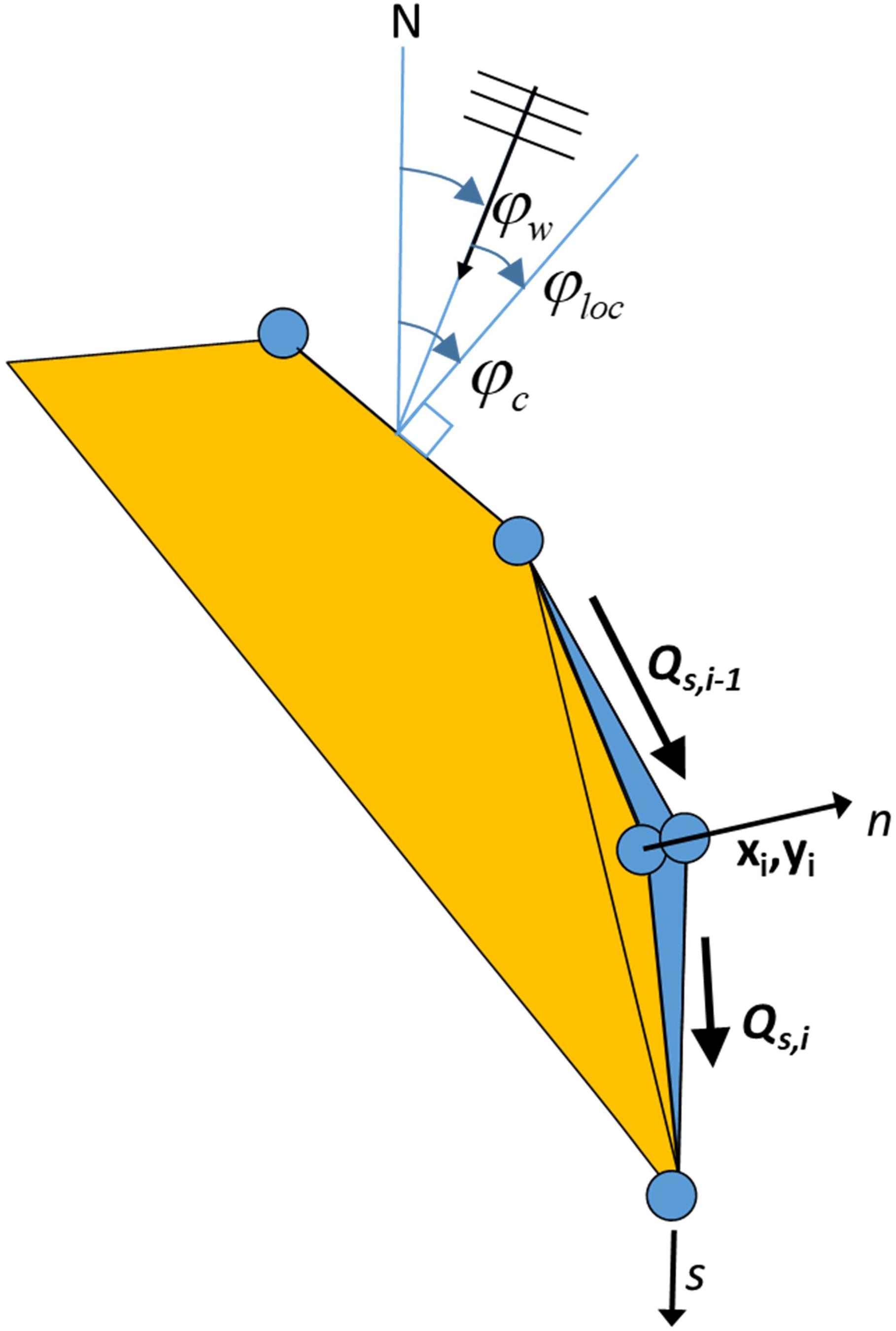
Figure 1. Coastline-following coordinate system and definition of wave and coast angles. φc is the orientation of the shore normal with respect to North; φw is the angle of incidence of the waves with respect to North and φlocthe local angle between waves and coast, defined as φc−φw.
Basic Equation
The basic equation for the updating of the coastline position is based on the conservation of sediment:
where n is the cross-shore coordinate, s the longshore coordinate, t is time, Dc is the active profile height, Qs is the longshore transport (m3/yr), tan β is the average profile slope between the dune or barrier crest and the depth of closure, RSLR is the relative sea-level rise (m/yr) and qi is the source/sink term (m3/m/yr) due to cross-shore transport, overwashing, nourishments, sand mining and exchanges with rivers and tidal inlets. In the Volume Balance section in the Supplementary Information we explain why equation (1) correctly represents the balance of both dry land area and the sediment volume, even for curved coasts.
Transport Formulations
The coastline changes are driven by wave-driven longshore transport, which is computed using a choice of formulations, which can be calibrated to match the local transport rates. The formulations listed in Table 1 have been implemented. The definitions of the angles are as in Figure 1.
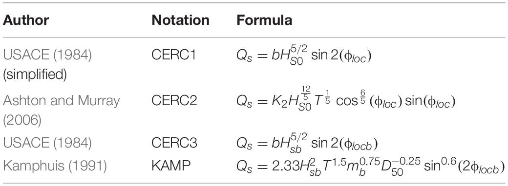
Table 1. Implemented longshore transport formulations.
CERC1 and CERC2 are defined in terms of the offshore wave angle, and CERC3 and KAMP are defined in terms of the breaking wave angle. However, in all cases the transport follows a shape rather similar to CERC1 when plotted against the deep water wave angle, with a maximum occurring at an offshore angle of 40° to 45° from wave incidence.
CERC1 is the simplest formula and is mainly meant for illustrating the principles of the behavior of the coastline model. CERC2 is derived from the official CERC formula to formally include the effect of refraction and shoaling. Though its behavior is quite similar to CERC1, it allows for a direct comparison with the Coastal Evolution model that utilizes it. The CERC3 and KAMP formulas are widely used in models worldwide such as GENESIS or UNIBEST and again can be useful for intercomparison with such models. CERC1, CERC2 and CERC3 have a single calibration coefficient, whereas the KAMP formula requires, usually uncertain, extra inputs such as beach slope and grain size but has the ambition to be a more accurate, predictive formula.
In Table 1, HS0 and Hsb are the significant wave height at the offshore location and point of breaking respectively (m), T is the peak wave period (s), D50 is the median grain diameter (m), mb is the mean bed slope (beach slope in the breaking zone), Φloc is the relative angle of wave incidence for waves offshore and Φlocb is the relative angle of waves at the breaking point; b and K2 are the calibration coefficients of CERC1 and CERC2 formulations respectively, which are computed as:.
where k is the default calibration coefficient according to the Shore Protection Manual USACE (1984), ρ the density of the water (kg/m3), ρs the density of the sediment (kg/m3), g the acceleration of gravity (m/s2) and γ the breaker criterion.
Numerical Implementation
The ShorelineS model is implemented in Matlab. The flow diagram of the model is depicted in Figure 2. In the following we will describe the procedure point by point.
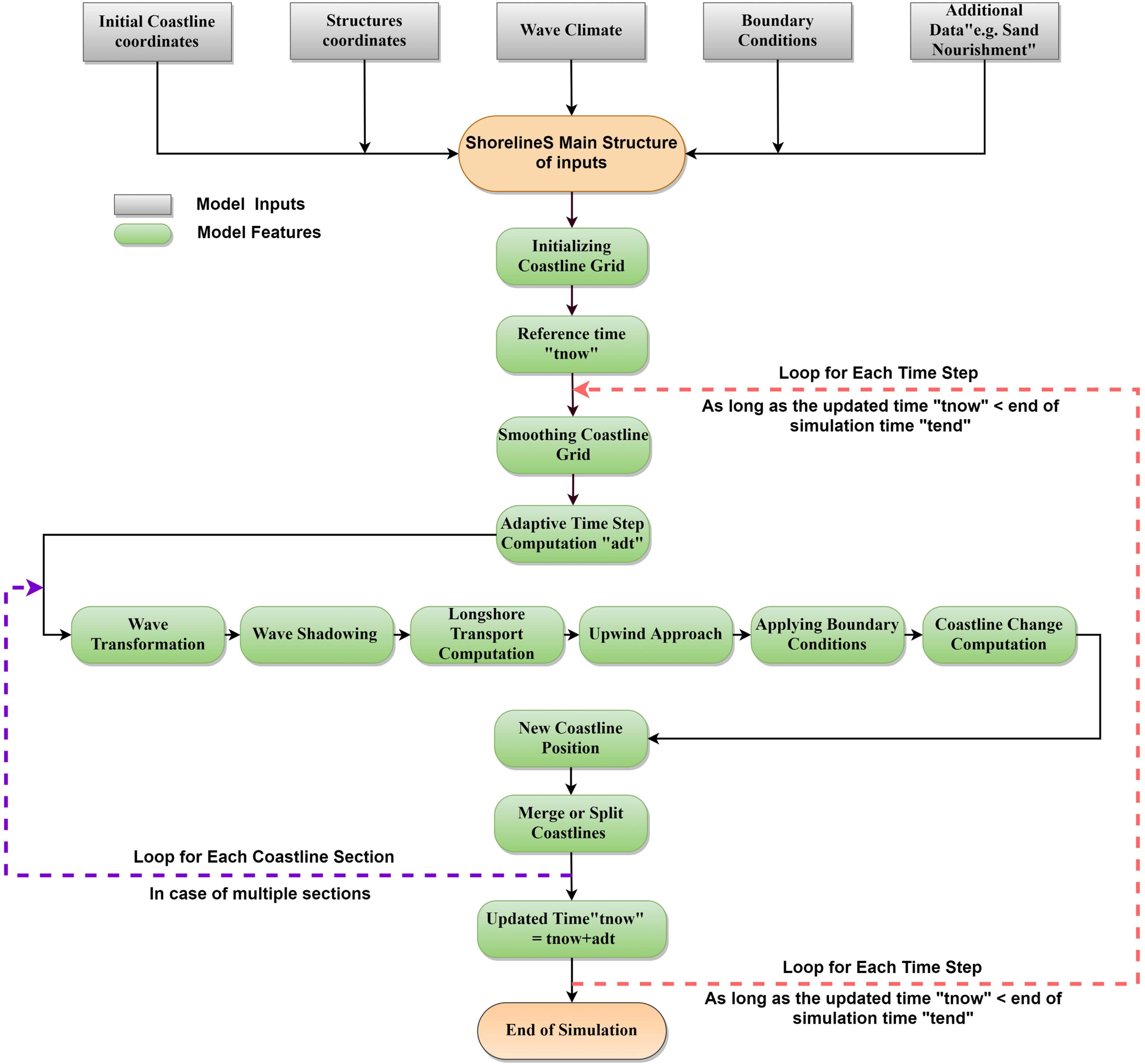
Figure 2. Flow diagram of the ShorelineS model.
The coastline positions are given in two column vectors xmc and ymc, where the different coast sections are separated by NaN’s. The sea is defined to the left when following the coastline positions. If a section ends at the same coordinates as where it starts, it is treated as a cyclic section and may represent either an island or a closed lagoon. The coordinates may be in any Cartesian (metric) system. Structures are defined in a similar way, as two column vectors where different structures may be defined, separated by NaN’s.
The offshore wave climate can be specified in three ways:
• By means of wave direction and a spreading sector, where a uniform distribution is assumed between the mean wave direction and plus or minus half the spreading sector. For each time step a random wave direction will be chosen from this sector.
• By a wave climate consisting of a number of wave conditions characterized by significant wave height, peak period and mean wave direction, each with equal probability of occurrence. A condition will be chosen randomly for each time step.
• By a time series of these wave conditions, from which the model will interpolate in time.
Various lateral boundary conditions were implemented in the model to represent a variety of coastal situations. For the non-cyclic sections the lateral boundary conditions are specified by controlling the sediment transport rate at the start and end of the boundary, thereby specifying a constant coastline position, a constant coastline orientation or a periodic boundary condition. One type of boundary condition is applied at all open-ended sections, whether existing or newly created. The model detects when a section end point is near the section start point and then always applies cyclic boundary conditions.
Nourishments can be prescribed through a number of polygons within which each nourishment takes place, start and end times, and the total volume of each nourishment. This information is then internally converted into a shoreline accretion rate by dividing the total volume by the time period, the length of coastline within the polygon and the profile height, Dc. By the same mechanism sediment discharged by a river can be distributed over a coastline section within a specified polygon. Shoreline recession as a result of relative sea level rise can be specified, e.g., resulting from the Bruun rule (Bruun, 1962), as given by eq. (1).
All inputs are collected in a single structure S that is passed on to the main function ShorelineS. Preparation of the input can be done in a tailor-made script, but ShorelineS and its sub-functions normally do not have to be altered for a specific application. The main function ShorelineS contains default values for all inputs that are not application-dependent.
The cumulative distance s along each coast section is computed, and this is then distributed over equidistant longshore grid cells based on a given initial grid size. The x and y positions of the coastline then are interpolated along s to obtain the x and y positions of the grid points.
In cases where the grid sizes expand (e.g., at the tip of an expanding spit), new grid points are inserted where the grid size exceeds twice the initial prescribed grid size. Where the grid distances shrink (e.g., at an infilling bay or a shrinking spit) grid points are removed when the grid distance becomes less than half the original grid size.
To avoid strong variations in grid size after inserting or extracting grid cells in expanding or shrinking sections, some smoothing of the s-grid is applied. The smoothing factor has to be chosen carefully as too much smoothing may lead to a loss of planform area and will tend to straighten out sections that should not move at all. The smoothing formulation applied is a simple 3-point smoothing according to:
where f is a smoothing factor, with default value of 0.1. Smoothing can lead to losses in the sediment balance and in situations where this is critical a value closer to zero is advised.
The local wave angle is estimated through the wave transformation from deep water to the nearshore using Snell’s law of refraction and from the nearshore to the breaking line using the equations of van Rijn (2014). The refraction from deep water to the toe of the dynamic profile can be done based on the assumption of parallel offshore depth contours, or using a 2D refraction model to provide alongshore-varying wave conditions.
Some parts of the coastline might be sheltered by structures or other parts (sections) of the coast. Hard structures or rocky shores are represented by an arbitrary number of polylines, which shield waves and block longshore transport where they cross a coastline. Thus, sea walls, hard rocks and headlands can represent supply limited situations where the transport is determined by the updrift sand supply and ‘plugs’ of sand are bypassed. The waves at any location can be shielded by other coast sections or hard structures, see Supplementary Figure SI01. This approach is valid when the scale of the structures is much larger than the wave length; if this is not the case, diffraction can be activated using different approximations (Elghandour, 2018).
Given the local wave angle with respect to the coast normal and the refracted wave conditions (or deep water wave directions in the case of the CERC1 and CERC2 formulas) the longshore transport can be computed at each transport point between two adjacent coastline points. At present, a choice of formulations as listed in Table 1 is available to be used.
Coastline Evolution
At each point the local direction of the coast is determined from the two adjacent points (as a reference line), then the longshore transport is calculated for each segment. The difference leads the points to build out or to shrink. The mass conservation equation is solved using a staggered forward time–central space explicit scheme (see Figure 1):
where j is the time step index, Δtis the time step (yr), i is the point/node index and Li is the length of the considered grid element computed from and xi and yi are the Cartesian coordinates of point i. From the normal displacement it follows that the change in position of point i then becomes:
The scheme can be shown to be conserving the land area. Since an explicit scheme is applied, the time step is limited by the following criterion (Vitousek and Barnard, 2015):
where the diffusivity ε is related to the maximum gradient of the sediment transport with respect to the wave angle relative to the coast, which can be approximated by:
where Qmax is the maximum transport rate in the model.
Therefore the following is obtained:
This criterion can be restrictive for small grid sizes (e.g., less than 100 m). Stability is, however, guaranteed through this adaptive timestep.
High-Angle Instability
A special treatment takes care of so-called high-angle instability (Ashton et al., 2001), which allows spits to develop. In cases where the local angle exceeds the critical angle on one side and is less than the critical angle at the updrift side, the transport at the downdrift point is set to the maximum transport (or the angle is set to the critical angle). Figure 3 illustrates the effect of this treatment, where a central scheme would lead to unstable behavior, the local upwind treatment ensures a smooth development into a spit. The physics in the model is the same as in Ashton et al. (2001, 2016), and Ashton and Murray (2006), and therefore it inherits most of the behavior of their Coastal Evolution Model. The novelty in ShorelineS is that it achieves the same behavior with a vector-based rather than a grid-based approach. This is more elegant and more efficient, especially when large areas need to be covered.
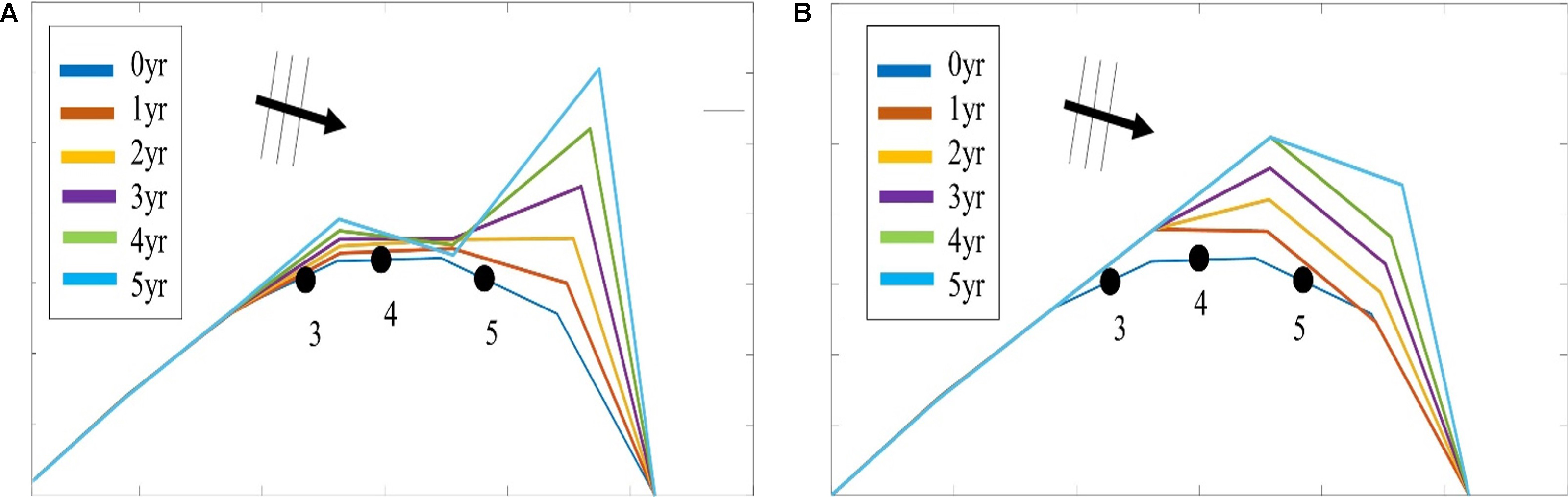
Figure 3. Example of high-angle instability with standard central scheme (A) and upwind scheme (B).
Barrier or Spit Overwash
For simulating barriers that already exist or that are in the form of developed spits due to high wave angle instability, it was necessary to represent the overwash process as it maintains the width of the barrier to a certain limit (Leatherman, 1979).
(Ashton and Murray, 2006) introduced the physical process of overwash by assuming a minimum barrier width such that sediment eroded from the seaward side is deposited on the landward side. By simultaneously retreating the seaward and landward sides of a section narrower than the specified critical width, the retreating section creates a longshore transport gradient that tends to fill it up; thus, the retreating helps maintain the width.
A similar concept was implemented in ShorelineS in a simple approach for treating the barrier width. At each time step, the model checks the local barrier width at each point/node, measured in the incident wave direction. If the barrier is narrower than the critical width, then overwash occurs. The overwash process moves the landward point a distance equal to the difference between the actual width and the critical width. Such a distance is not allowed to exceed a given percentage (e.g., 10%) of the local spatial discretization distance of the grid per time step to avoid discretization artifacts. Then the model looks for the closest node on the seaward side to erode it by the same amount (Supplementary Figure SI02). A possible refinement is, as in Ashton and Murray (2006), to assume different profile depths on the seaward and landward sides, as is logical in some settings, e.g., for the case of an eroding barrier island. In this case the landward extension would be larger than the erosion on the seaward side.
Merging and Splitting
One of the advantages of the ShorelineS model is that it can simulate multiple coastal sections at the same time, and these sections can affect each other by shielding the waves. Small parts of the coast are allowed to split and migrate as the spits are growing and in some cases break up and migrate as a small island. An example of the splitting procedure is shown in Supplementary Figure SI03. Such splitting typically happens when the seaward side of a section erodes by more than the overwashing process allows for or when the latter is not activated. The numbering is indicated to show how the grid cell connections change after the splitting procedure: from one continuous coastline section to two separately numbered sections.
If two sections intersect, they may merge into one section as the simulation continues, as is illustrated in Supplementary Figure SI04. Such merging typically happens due to shoreward migration or extension of a spit toward the mainland coast. Again, the numbering is included to indicate how the separate spit and mainland coast sections are now joined at the seaward side as a continuous coastline numbered 12-20 and a lagoon numbered 1-10.
Treatment of Groins
Groins can be treated simply as any structure crossing the coastline, where the transport at the transport point closest to the intersection between the structure polyline and the coastline is set to zero. However, such a treatment does not give a very accurate representation of the groin position and local coastline evolution, and does not account for bypassing in a smooth way. Therefore, a more eleborate treatment was presented in Ghonim (2019), which is summarized as follows. First, additional grid points exactly on either side of each groin are introduced. Second, the local coastline position at either side of the groin is forced to move along the groin. Third, bypassing and transmission are accounted for, according to the following mechanisms.
Bypassing can be simulated in two ways, either as starting only when the updrift accretion has reached the tip of the groin, or gradually increasing if the depth at the tip of the groin is less than the depth of active transport. The first approach follows the considerations of, assuming a fully impermeable structure, such as a groin with complete blockage of the longshore transport. Sand bypassing takes place only when the groin is filled with sand. Based on that, the longshore sediment transport is set to zero at the structure and the sand bypassing factor (BPF) also is set to zero from the start of the simulation until the moment when the sediment reaches the tip of the groin. Then, the bypassing factor is set to its maximum value (BPF = 1), which means that all sediment bypasses the groin’s tip and moves towards its downdrift side. In that case the lateral boundary condition at grid point i (see Supplementary Figure SI05), which is located at the groin representing the bypassed volume can be expressed as:
where QSi is the longshore transport at grid point i. There were many options for how the bypassed sediment should be distributed downdrift of the groin. The most appropriate distribution of the bypassed sediment, in line with the expected flow pattern around the groin, which attaches roughly at the end of the sheltered area, is to pass all the bypassed sediment at the last sheltered grid point ilast and to leave the sheltered area untouched. To do so numerically, the lateral boundary conditions at the downdrift side of the groin are set as follows:
Eq. (11) ensures that only the last sheltered grid point obtains all the bypassed sediment and equal signs indicate that there is no sediment transport gradient from the grid point i to the last sheltered grid point ilast. This approach keeps the sheltered grid points fixed in their positions except for the last one, which gives a transport gradient to its following grid point.
That this treatment is more realistic than the classical Pelnard-Considère solution where an erosion peak at the downdrift end of the groin is assumed follows from many examples worldwide, where the erosion peak is rarely found right next to the groin but always some distance downdrift, due to the wave sheltering and recirculation in this area. An example is shown in Supplementary Figure SI06, for a groin field at Eastbourne, United Kingdom.
The second approach (Larson et al., 1987) assumes that sand bypassing does not take place only when the groin is totally filled with sand, but it may take place just after the construction of the groin. While sand moves along the coastline, it is influenced by the presence of the shore-normal structures, such as groins and the response of the coastline to those structures varies for different locations and different types of structures. The main parameters that influence the response of the shoreline at the structure are the structure permeability and the bypassing ratio, which is the ratio between the water depth at the head of the structure Ds and the water depth of the active longshore transport DLT. The bypassing ratio varies between 0 and 1 (Hanson and Kraus, 2011).
Sand bypassing occurs at the seaward end of the groin as long as Ds is less than DLT. The depth of the active longshore transport is similar to the depth of the highest 1/10 waves at the updrift side of the structure (Hanson, 1989), and represents the time-dependent depth for longshore sediment transport, which is often less than closure depth Dc, and can be estimated as:
where Aw = 1.27, a factor that converts the 1/10 highest wave height to significant wave height [-]; γ is the breaker index, the ratio between wave height to wave depth at breaking line [-] and (H1/3)b is the significant wave height at the line of breaking [m].
Based on the assumption of equilibrium profile shape (Dean, 1991), the water depth at the structure’s head Ds can be determined as:
where Ap is the sediment scale parameter [m1/3] and ystr is the distance from the structure’s head to the nearest point of the coastline [m]. In that case, the bypassing factor (BPF) is estimated based on the following equation:
and the bypassing volume increases until reaching its maximum value when the groin is filled with sediment [BPF = 1]. The lateral boundary conditions at the groin are otherwise equal to those for the first approach, as given by Eqs. (6) and (7).
Analytical Tests
A number of analytical tests were done to verify the correct implementation of the governing equations and the numerical scheme. They are described extensively in Elghandour (2018). Here, for brevity, the results are summarized for only two of these tests.
Linear Diffusion Test
The first test is the verification test used by Vitousek and Barnard (2015) to validate the CoSMoS model. The shoreline starts with the configuration y = acos(kx), where k = 4π/L and the analytical solution of the shoreline evolution is y = aexp(−vk2t)cos(kx) where v = 2Qo/Dc. The model was run with an adaptive time step based on the criterion Δt < Δx2/2ν. The amplitude of the shoreline perturbation was 100 m, the domain length 5 km, the wave angle 0°. Qo was taken at 105 m3/yr, the space step was 50 m and the total simulation time 30 yr. The resulting evolution is stable and accurate, see Figure 4.
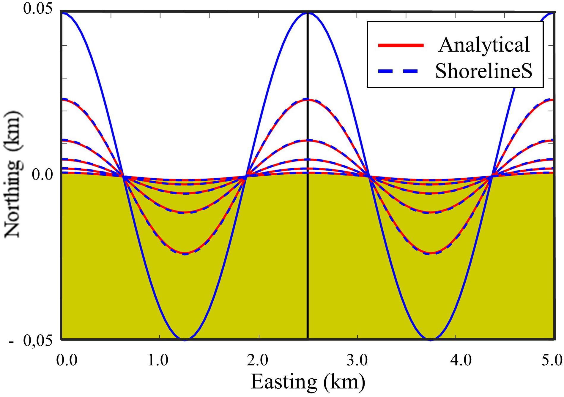
Figure 4. The diffusion test result using the adaptive time step; results shown every 6 years.
Pelnard-Considère Groin Test
This test reproduces the well-known analytical solution for the accretion and erosion on either side of a groin on a uniform coast, according to Pelnard-Considère (1956). However, the validity of that solution ends when the updrift side of the groin is completely filled with sand or when the incident wave angle is too high. Both bypassing approaches were tested with different incident wave angles. As expected, the first approach has produced a perfect agreement with the analytical solution for a wave angle of 10° (see Figure 5A), while a slight difference in the shoreline position is observed for a wave angle of 25°, at which the analytical solution loses its validity and overestimates the rate of change in the shoreline position (see Figure 5B). That difference increases when applying the second approach, due to the partial bypassing which slows down the shoreline movement; moreover, the difference downdrift of the groin is due to the effect of the wave shadowing which is not taken into account in the analytical solution (see Figure 5C).
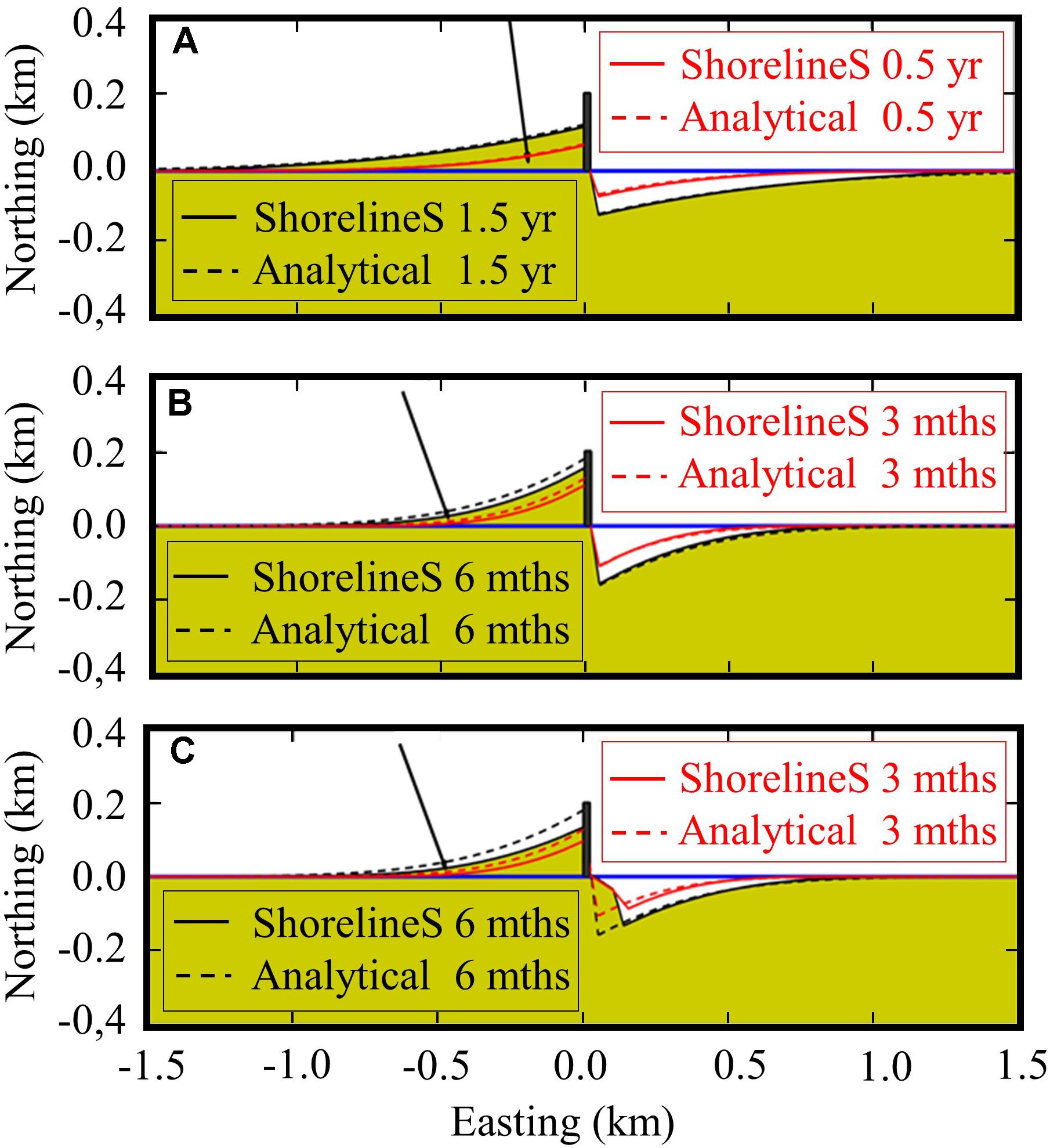
Figure 5. Shoreline response for both the analytical solution and ShorelineS with different wave angles and bypassing approaches. Panel A: incident angle 10°, no shadowing; panel B: incident angle 25°, no shadowing; panel C: incident angle 25°, with partial bypassing and shadowing.
Overall it may be concluded that the comparison with analytical test cases is satisfactory, both for the diffusion test and the groin case, and that the basic equations and numerical scheme have been implemented correctly.
Principle Tests of Complex Behavior
Island Deformation
This test was designed to investigate the behavior of a deforming island under different wave spreading and spit overwashing scenarios. The initial coastline is a perfect circle with a radius of 500 m. The mean wave direction is from the West, 270° N. A wave height of 1 m and a transport coefficient of the CERC1 formula was applied, leading to a maximum transport of 1 Mm3/year. The simulation ran for 4 years in all cases. The wave spreading varied between 0°, 90°, and 180° and the grid resolution was 50 m.
For the case without wave spreading two long and narrow spits extend from the island, under the theoretical (Ashton et al., 2016) angle of 45° relative to the wave propagation direction. In the case where no spit overwashing is allowed the section of the spits nearest to the island becomes thinner and at some point breaches; this process repeats itself. The overwashing process paradoxically ensures the survival of the spit as the landward migration attracts sediment due to the longshore transport gradient that is created by the local retreat due to overwashing. In Figure 6 the effect of the critical spit width is illustrated. In the left panel, without the overwash mechanism, the spit breaks apart; the overwashing with spit width of 100 m (middle panel) or 200 m (right panel) clearly leads to more robust spit behavior. For the case with 90° spreading the coastline is more curved and the spit wider because (a) waves can initially reach further around the island and (b) the transport can get around the tip of the spits more easily during the conditions most perpendicular to the spit. For the case of 180° spreading the spits cannot fully develop and are wrapped around the island, which turns into a retreating, jellyfish-like shape. For the cases with larger spreading the spit overwashing has a much less dominant effect.
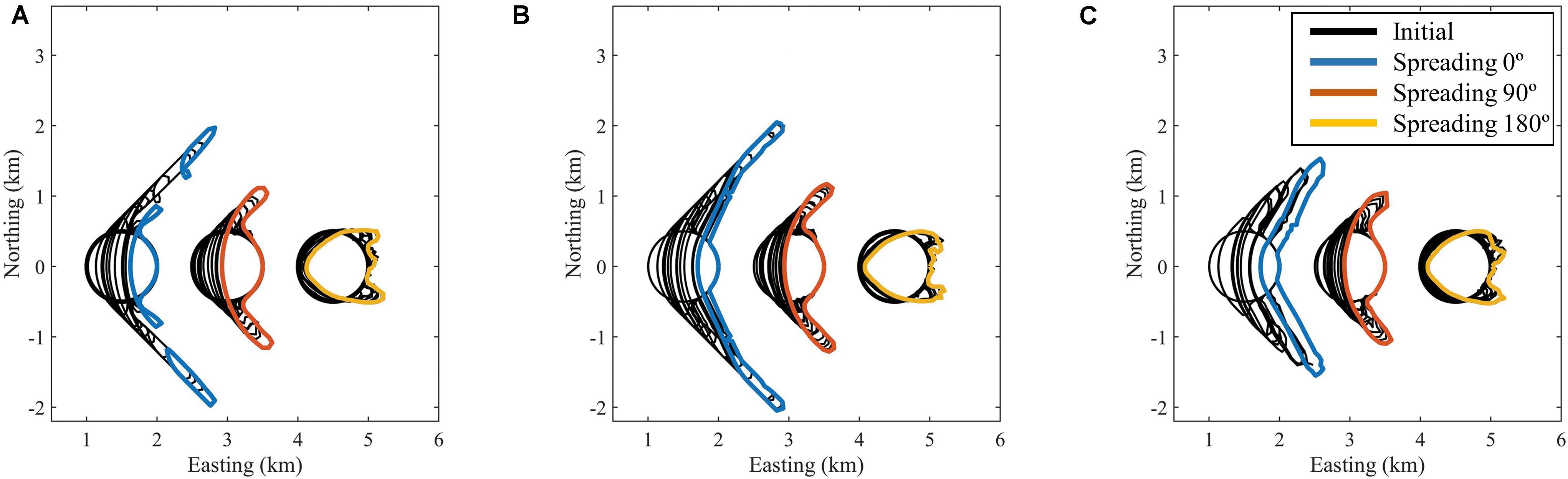
Figure 6. Deformation of an island due to waves with mean direction from the West; wave spreading uniform 0°, 90°, and 180°, respectively. Left panel (A): no overwash. Middle panel (B): critical spit width 100 m. Right panel (C): critical spit width 200 m.
Island Merging
This test has been designed to examine the model stability and behavior under the merging and splitting of different coastal sections. The initial island configuration and the wave conditions and other settings are the same as in the previous test case, but now the island is located 800 m from a straight beach facing West. The duration of the simulation is 10 years in this case. In Figure 7 the process of island deformation, migration to the coast and welding with the coast is illustrated for the case of a critical spit width of 100 m. In the top panels, the case of no directional spreading shows the formation of a lagoon after 2 years. The barrier overwash procedure allows for the rollover of the barrier enclosing the lagoon, leading to a rapid landward migration and welding of the barrier with the original coastline, after which the island has interestingly left two distinct humps and two small lagoons on the original coastline. A similar process, though slower and with less longshore extent, takes place with the higher spreading of 90°. In this case one extended lagoon remains. Finally, for a large directional spreading of 180° the island as a whole migrates onshore and welds to the beach, leaving only a small lagoon. Since the island is shielding northerly wave directions in the South and southerly directions in the North, it also acts like an offshore breakwater, attracting sand behind the island at the cost of erosion at some distance. For this case the final coastal shape is quite stable, as the southern part is oriented toward waves from the South and shielded from those from the North and vice versa.
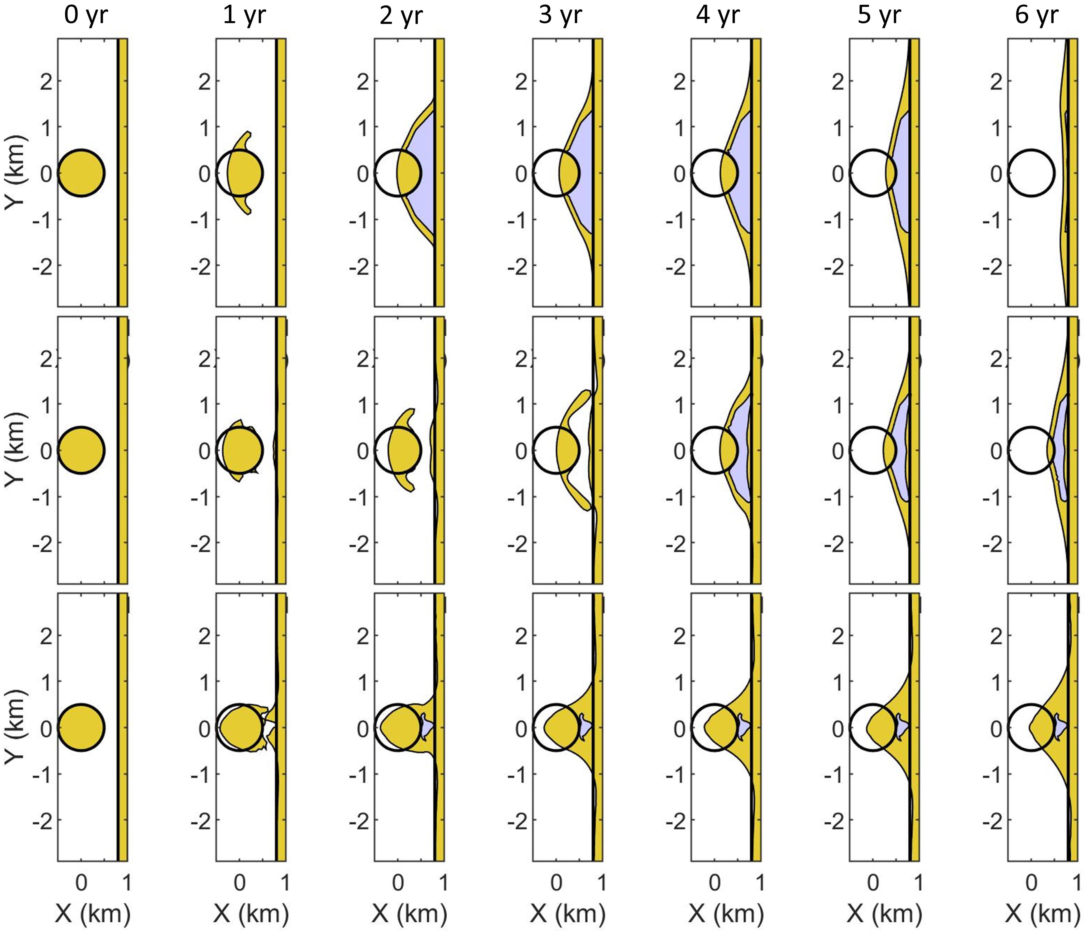
Figure 7. Evolution of an island merging with the coast, for a critical spit width of 100 m. Top row: directional spreading 0°; middle row: 90° and bottom row: 180°. Time between subsequent figures approximately 1 year.
These developments appear to be realistic and demonstrate the capability of the model to evolve coastal shapes through significant changes. Welding of a spit to the coast is frequently observed, as in, for instance, the case of the Sandmotor, shown in Section “FIELD VALIDATION.” Configurations such as the final one for a spreading of 180° are commonly seen when the wave climate has a large spreading, as for instance for the island heads in Zeeland, in the south of the Netherlands. A jellyfish-like shape migrating in the wave propagation direction as seen in the bottom panels of Figure 7 and the right-hand shapes of Figure 6 are clearly visible in, e.g., the Noorderhaaks, a sandy island between the coasts of North Holland and Texel in the Netherlands.
Flying Spits
In order to test the model performance under a high angle of wave incidence, and to verify the model ability to grow spits through the instability mechanism according to Ashton et al. (2001), the test conditions follow the numerical test introduced by Kaergaard and Fredsoe (2013b). For this test the initial grid size = 250 m, spit width = 250 m, closure depth = 15 m and the CERC2 formula was applied; the total simulation time was 250 years. The total shoreline length was 100 km, the initial undulation length was set to 5 km and the initial amplitude of the undulation was 50 m. The wave conditions were kept constant at a wave height of 1 m, a peak wave period of 5 s and a mean wave direction of 300°.
Periodic boundary conditions were used to the left and Neumann boundary conditions were used on the right boundary. Figure 8 shows a section of 50 km in the middle of the test coastline at different stages. We clearly see the initial disturbances grow into wave-like patterns, which grow and merge into larger length scales, and finally reach the stage of flying spits, from which even small islands can be detached.
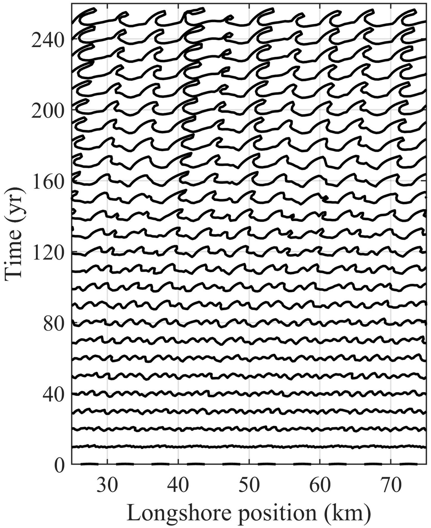
Figure 8. Shoreline undulations under test conditions of Kaergaard and Fredsoe (2013a).
The single high angle wave direction leads to small protuberances, which accrete forming larger bumps (around 100 years) and the bumps’ crests evolve while the flanks retreat. This continues until they reach the point when the shoreline angle is equal to the maximum transport angle, when the upwind correction applies so that a spit forms. The shoreline angle at the up drift side increases but cannot exceed the maximum transport angle. The spit evolves to the down drift direction. As shown in Figure 8, after a while sometimes breaching might occur at the spit neck so small islands can be detached. Part of the shoreline at the down drift side of the spit is shadowed from the approaching waves; that feature does not change after spit formation. This is not always the case in reality as it might be filled up by aeolian transport, due to overwashing or due to wave approach from the down drift direction.
As the spit extends offshore, the spit tip migrates toward the down drift direction and repeatedly a new spit tip forms, taking over the old tip. The spit migration speed is 28 m/yr on average. The growth rate of the spit was approximately estimated to be 15 m/yr at Walvis Bay, Namibia according to Elfrink et al. (2003).
Though different in details from the results of Kaergaard and Fredsoe (2013a) we also see the development of the spits with a wave length in the order of 5 km after approx. 120 years; their model includes nearshore wave refraction over the evolving bathymetry and thereby suppresses smaller-scale disturbances apparent in our model.
Overall the growth rate is slower than estimated by the model presented by Ashton and Murray (2006); the reason for the slower growth rate is mainly that the transport coefficient they applied leads to sediment transport in the tens of millions of m3/yr, which is not realistic.
In natural conditions, the entire coast is affected by multiple wave approach angles and also the alongshore boundary condition impacts the evolution behavior. More complicated conditions and real cases will be the subject of further studies. The current case, however, shows that the new numerical approach is capable of reproducing similar flying spit features as in both Ashton and Murray (2006) and Kaergaard and Fredsoe (2013a).
Van Rijn’s Compendium of Coastal Forms
The following case is inspired by the picture in van Rijn (1998), see Figure 9. It describes a compendium of coastal features, based on the author’s experience, and the authors’ ambition was to re-create most of them in a single simulation, highlighting that any coastal shape predominantly created by wave-driven longshore transport can be produced by the proposed model.
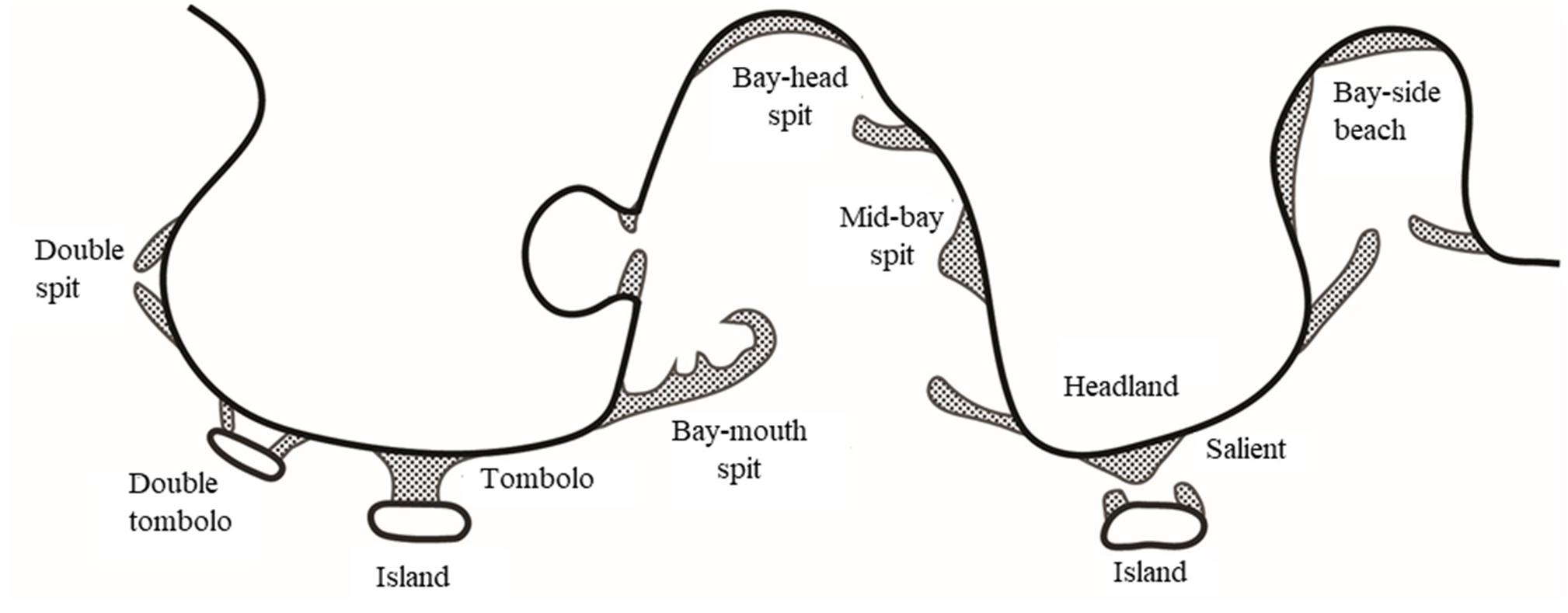
Figure 9. Overview of sandy coastal shapes, from van Rijn (1998).
The initial setup is shown in the top panel of Figure 10. It contains a coast with sharp variations in orientation with a sandy island and two hard offshore breakwaters or rocky obstacles. The wave climate is from the South with a constant offshore significant wave height of 1m and a random spreading of 120°. The CERC1 formula was used, with a coefficient b of 1 Mm1/2/yr. The grid resolution was 200 m and a fixed time step of 1/50 yr was applied. The profile height was taken as 6 m and the critical spit width was taken as 100 m. We see a number of spits developing, on the sides of the island and on all protruding parts of the coast ‘bay-mouth spits’ can be seen (Figure 10). After 20 years the island spits weld to the coast creating a lagoon. The western breakwater captures the westward longshore transport, creating a tombolo. After 50 years the central spits merge together and start extending seaward, while the island has fully disappeared, its sand distributed along the eroding coast. On the western coast the headland spit has welded to the coast, creating a curved embayment with an enclosed lagoon.
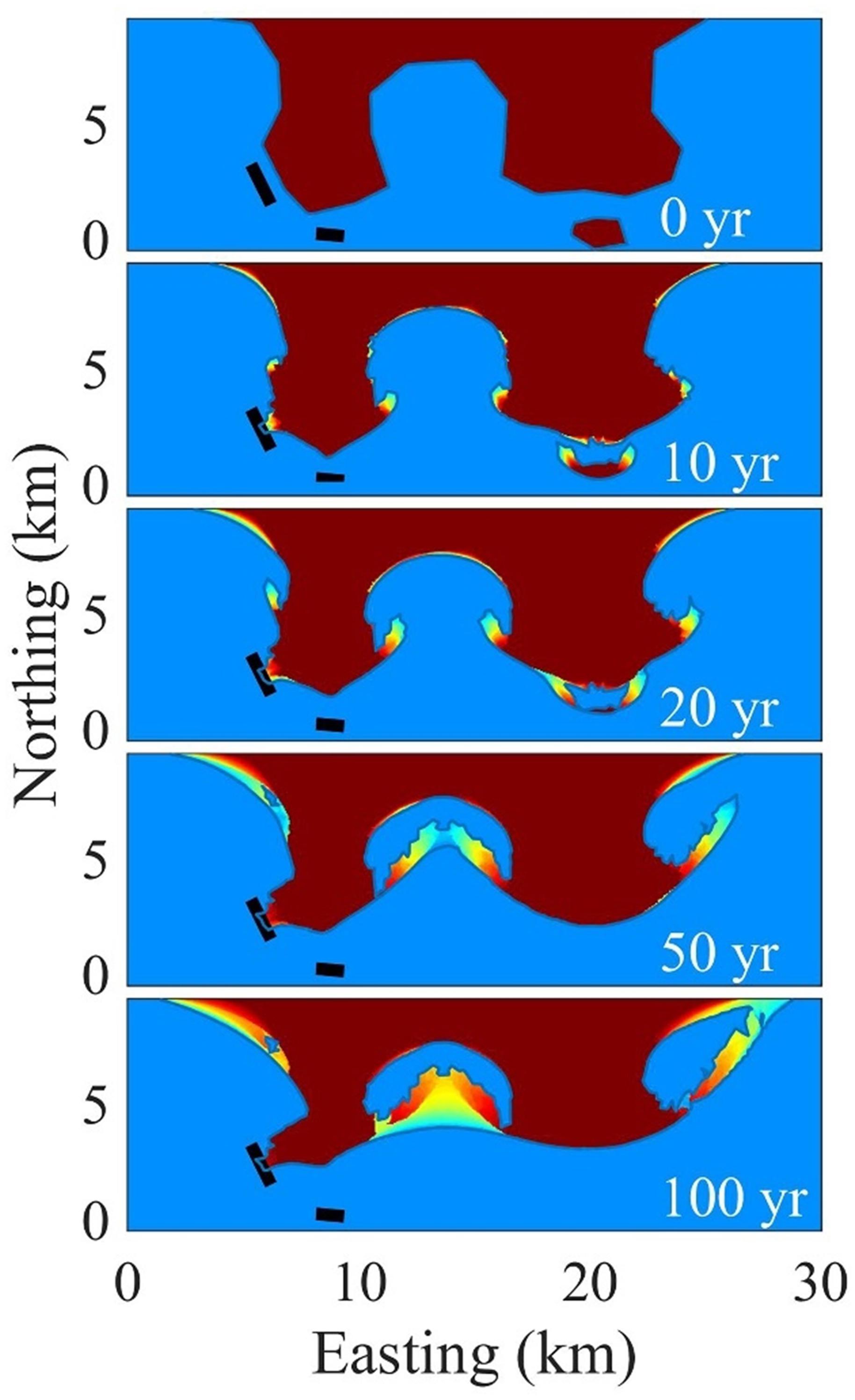
Figure 10. Evolution of coastal features in a geometry resembling van Rijn’s overview of coastal shapes. Colors indicate age of deposition, with green the most recent deposition to dark red for the oldest deposition.
These developments seem quite realistic and intermediate shapes bear substantial resemblance to the sketches in Figure 9. They form an illustration of the capability of ShorelineS to represent not just incremental coastal changes, but radical transformations of the coast over long timescales.
The coloring of Figure 10 is done through post-processing on a fine grid, where for each pixel a record is kept of when it has become land or sea. This representation facilitates a comparison with observed horizontal stratigraphic features such as beach ridges.
In order to test the sensitivity of the model, in this case involving drastic transformations, to the grid resolution an additional test was done with half the grid size, e.g., 100 m instead of 200 m. The resulting evolution over the first 50 years is shown in Supplementary Figure SI07. Qualitatively, the same features are generated and on several elongated coastal stretches the differences are quite small. Because of the random variation of wave conditions, the differences are relatively larger in the beginning than at the end of the simulation; largest differences occur near the tips of spits, as would be expected.
It may be concluded from this test case that ShorelineS is capable of producing a range of observed coastal features, just based on an initial coastal configuration. Whether ShorelineS also predicts the properties of these features and the rate of change of their evolution correctly will be the subject of further study. In the following, two field case studies are given that show a (still limited) validation of this capability to quantitatively predict coastal evolution for complex cases.
Field Validation
The capability of ShorelineS to represent real-world coastal evolution is illustrated through the example of the Sand Engine (Stive et al., 2013; de Schipper et al., 2016), as well as for a groin scheme at Al-Gamil Beach, Egypt. Especially, the appropriate representation of rates of change (i.e., transport rates and subsequent gradients) and the shape of the coastline are considered essential properties of a shoreline model.
Sand Engine, Ter Heijde, the Netherlands
The Sand Engine is a large-scale sand nourishment (21 million m3 of sand) which can also be seen as a temporary land reclamation. The hydrodynamics and morphology at the Sand Engine have been the subject of intensive modeling efforts with 2DH process-based models (Luijendijk et al., 2017; Huisman et al., 2018), 1D line models (Tonnon et al., 2018) and hybrid approaches (Arriaga et al., 2017), all of which take considerable time to set up, calibrate and run (run times of up to months), and require a high level of expertise. The results are reasonable after considerable tuning, but only the most expensive process-based approach leaves behind a lagoon after the spit has merged with the mainland. Furthermore, typical coastline models represent either the shape (e.g., Ashton et al., 2001) or transport rates (Tonnon et al., 2018) well, but seldom perform well for both.
The ShorelineS model, on the other hand, requires only the initial, complex coastline and a nearby deep water wave climate. The latter is given as a probability distribution of (50) wave direction bins, each with equal total energy flux, with one wave height class per direction, as depicted in Supplementary Figure SI08, since an accurate representation of the directional wave climate is the most important aspect in the schematization. The shape of the distribution is constant in time. Dots indicate offshore measurements over a 10-year period. Each bin (contained in the red boxes) contains the same total energy flux and the representative wave height for each bin is denoted by the red dots. Each time step a wave condition is selected randomly from these 50 conditions.
The initial model resolution was set at 100 m. After this the only tuning needed was of the transport magnitude (formula CERC1, b = 500,000 m1/2/yr/rad), and the profile height (10 m). These parameters only influence the speed of developments, not the shape.
The results of the Sand Engine forecast (Figure 11) qualitatively reproduce well the shoreline reshaping over time and quantitatively reproduce the observed behavior, at minimal runtime (approximately 15 min). Even the shape of the spit is reproduced well in the model showing a smooth elongated connection to the mainland in September 2016 similar to the field observations. The temporal development of the erosion (middle panel in Figure 11) obviously misses the seasonal component (with sudden steps of erosion due to storm events) which is due to the use of an average climate, but the use of a temporally varying nearshore wave climate would also allow for the computation of the steps over time.
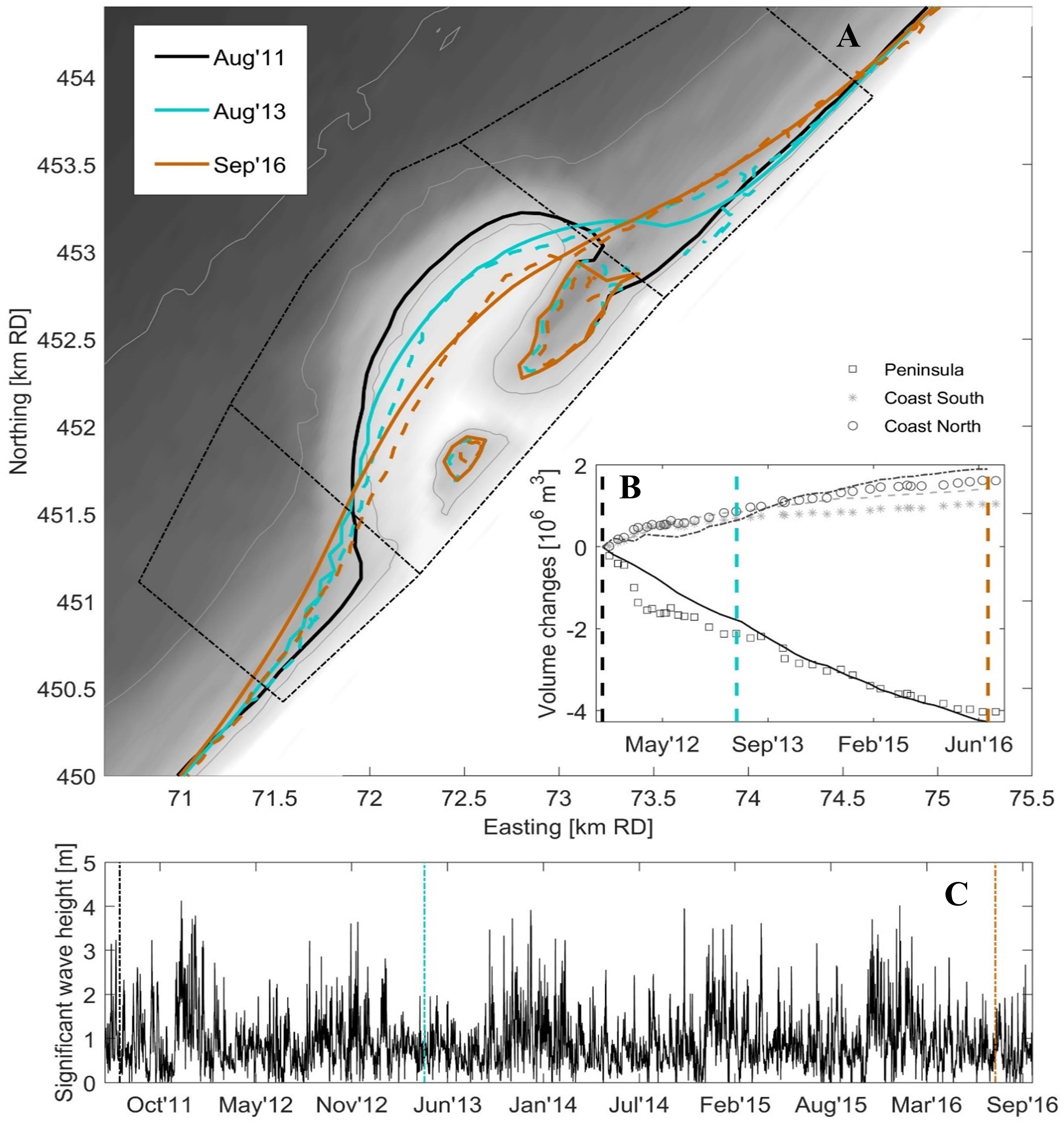
Figure 11. (A) Observed and simulated evolution of the Sand Engine using ShorelineS; Color-coded lines are coastlines extracted from repeat topo-bathymetry surveys (drawn lines) and from calculations (dashed lines) for 2011 (initial), 2013 and 2016. (B) Observed and computed volume change for the areas indicated by the black dash-dot lines. (C) Time series of actual significant wave height.
To quantitatively assess the performance of the model the distances distmess(t)–initial between two observed coastlines and between the observed and computed coastlines at a given time, distcomp(t)–meas(t) are computed. These distances are assigned a positive sign when the coastline moves seaward and negative when it moves landward. The following parameters:
In these parameters, biasm denotes the net measured shift of the coastline (positive seaward), rmsm the root-mean- square deviation of the measured coastline, biascm is the net shift between measured and computed coastline positions, rmscm is the root-mean-square difference between measured and computed coastline and BSS is the Brier Skill Score, a measure of the model skill frequently used in morphodynamic modeling, e.g., Figure 12 shows an example of this computation, with the observed and computed coastlines in the left panel, along with their error parameters, and the distances as a function of the alongshore distance in the right panel. Region A shows accretion in measurements and computations, Region B has a huge erosion. Region C is the area where the spit welds to the coast and then spreads North. In region D the lagoon that is formed by this welding is seen. Region E includes the original lake that does not move much. The rms error between measured and computed coastlines at this time is 42 m, whereas the rms difference between the initial and measured profiles at the same time is 144 m. In Figure 13 the development of the errors in time is visualized, showing that the error between observations and computation increases slowly in time, whereas the observed change keeps increasing; hence, the skill, as represented by the Brier Skill Score (BSS) commonly used to assess morphological model results, increases from 0.22 in the first half year to 0.65–0.7 and remains relatively constant. The relatively low skill in the beginning is due to a combination of the occurrence of a very stormy season and a low signal to noise ratio. According to the classification given by Sutherland et al. (2004) the skill develops from good (0.2–0.5) to excellent (0.5–1.0).
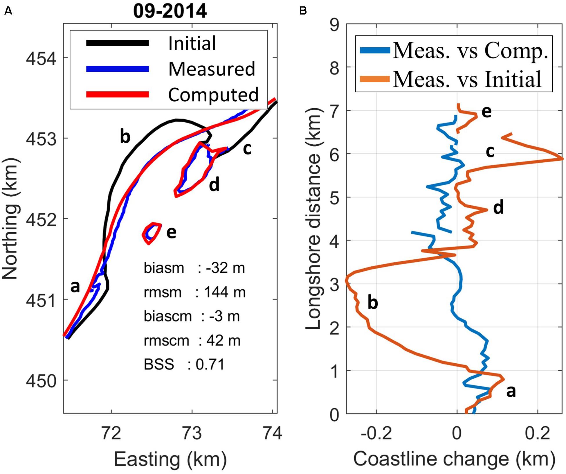
Figure 12. Initial (2011), measured (meas.) and computed (comp.) coast lines after 3 years (A); coastline change vs alongshore distance: measured vs computed, and measured vs. initial (B) Letters in both panels indicate the corresponding areas.
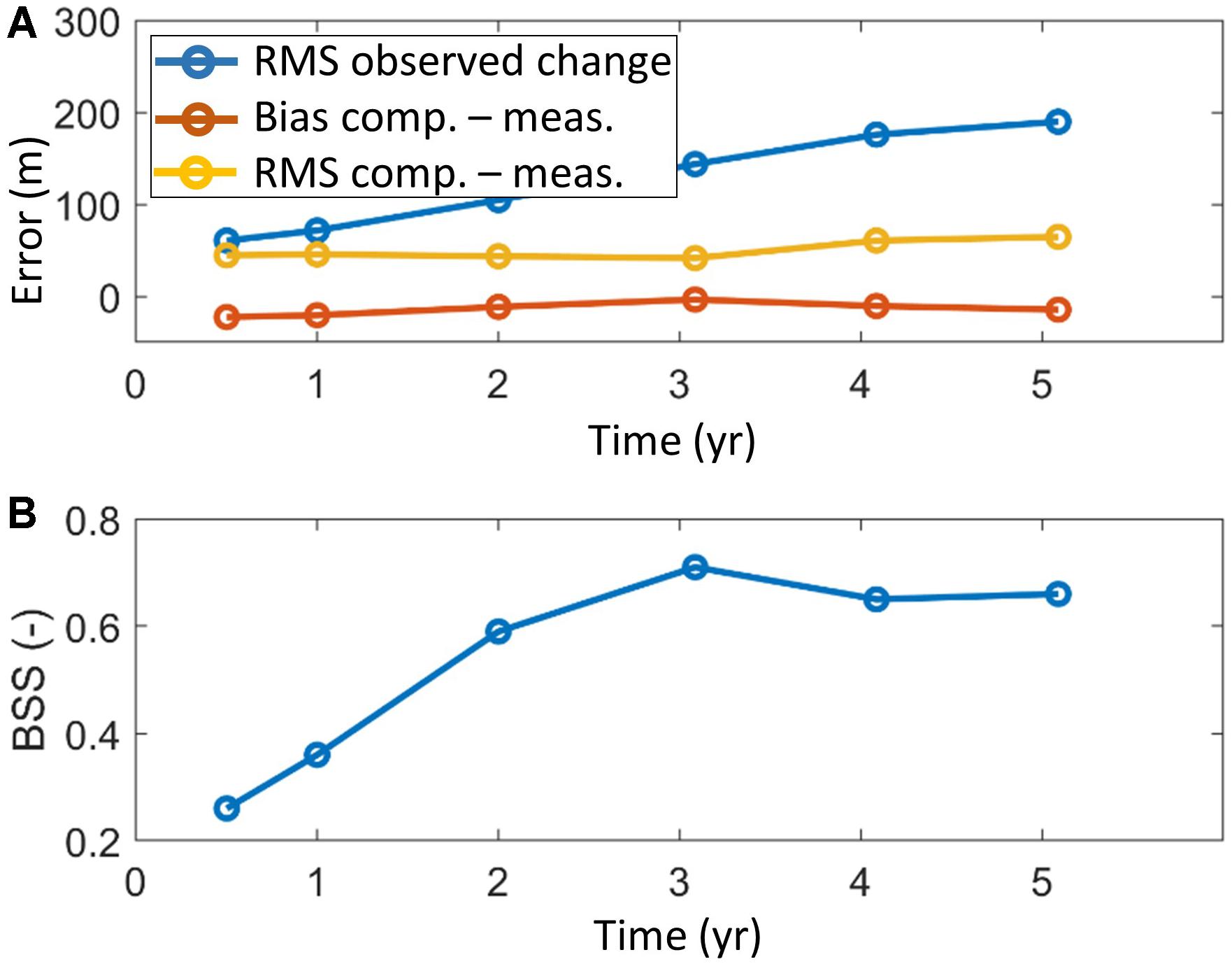
Figure 13. Bias between computed and measured coastlines, rms observed change and rms error vs time (A); Brier Skill Score (BSS) vs. time (B).
Application at Al-Gamil Beach, Port Said, Egypt
The main aim of this application is to validate the model in simulating shoreline response within a groin field where sand nourishment with different nourishment rates has been placed along the groin field. Moreover, it is aimed to evaluate the effect of the sand bypassing introduced through the new treatment of the groins, as discussed in Section “Treatment of Groins” and (Ghonim, 2019) in obtaining more realistic results. Data for this case were obtained from the Egyptian Shore Protection Authority through personal communication.
Background
Port Said is a coastal city located in the North-East of Egypt and stretches about 30 km along the Mediterranean Sea. Supplementary Figure SI09 shows the study area which is located west of the city and lies between (31°16′52.6″N, 32°14′48.43″E) and (31°16′33.31″N, 32°17′05.96″E). The existence of a tidal inlet in the west of the area causes imbalances in the longshore sediment distribution as it works as a sink, where the longshore drift tends to be deposited inside the inlet. This has caused erosion problems in the study area which is located downdrift of the tidal inlet, given that waves are dominantly approaching the coast from the North-west direction. A groin field that consists of 14 groins with different lengths varying from 80 to 50 m, and constant spacing of 170 m was constructed from 2010 to 2011 to minimize the erosion in that area. Moreover, a sand nourishment of around 125,000 m3 was placed in the spaces in between the western 6 groins, while approximately 75,000 [m3] of sand was nourished in the areas in between the remaining groins since they are shorter, so as to accelerate the effectiveness of the groin field in countering erosion. In addition, 800 m along the downdrift side of the groin field were nourished with around 280,000 m3 of sand to compensate for the shortage of sediment there and to let the sand move naturally along the coastline. The nourishment work started just after the construction of the groin field and took six months to be completed.
Wave Climate and Historical Shoreline
The historical satellite images in Google Earth Engine were used to manually extract the groin field location and shoreline locations in 2011 and 2018 in World Geodetic System (WGS) 84; then, all coordinates were converted to Universal Transverse Mercator (UTM) coordinates. The wave climate of the ERA5 reanalysis with 0.25°× 0.25° resolution, produced by the European Centre for Medium-Range Weather Forecasts (ECMWF) was used to extract wave climate during the simulation period at a location 1 km offshore of the study area. The wave climate was schematized to 50 wave directions and their representative heights using the same method as for the Sand Engine case; the resulting distribution is shown in Supplementary Figure SI10, showing a dominance of wave directions from the North-west.
Model Setup
The initial coastline in 2012 and the groin field were introduced as land boundaries in UTM coordinates. The partial bypassing approach according to Larson et al. (1997) was used in this application as it gives a better representation of the real bypassing around groins. The model estimates the bypassing factor, BPF, based on the water depth at the tip of each groin Ds (Eq. 13) and the depth of the active longshore transport DLT (Eq. 12). The median grain size D50 is 0.20 mm as the Port Said coast is characterized by fine sand. The sand nourishment was introduced in the model as nourishment rates with start and finish dates, based on the applied nourishment volumes and the active profile height. An initial grid size of 25 m was chosen. Since the sand nourishment was introduced in the model within the first six months of the simulation, the nourishment rates were set to zero from the first of July 2012 until the end of the simulation. The nourishment volumes were 125,000 m3, 75,000 m3, and 280,000 m3 in between the western six groins, in between the remaining groins and along the area downdrift of the groin field, respectively. The width of the nourishment area in between the groins was set to 170 m representing the constant spacing between the groins, and 800 m for the area downdrift the groin field. The active profile height is the beach berm height plus the closure depth, Dc, which is equal to approximately 9Hs where Hs is the mean annual significant wave height (m). The period of the nourishment process was set to six months. The wave climate is discretized based on a probability distribution of 50 wave direction bins, each with equal total energy flux and one wave height class per direction as seen in Supplementary Figure SI10, At each time step, a wave condition was selected randomly from this distribution and the transport was estimated using the CERC1 formulation. The beach profile was estimated using a Dean (1991) profile, and the depth of active longshore transport is estimated every time step according to the wave height (Eq. 12). The partial bypassing method was chosen since the depth of active longshore transport frequently exceeded the estimated depth at the tip of the groins.
Model Results
The model results at the end of the simulation (2018) are shown in Figure 14. The figure also indicates the shoreline location extracted from the historical satellite images in Google Earth Engine in 2011 and 2018.
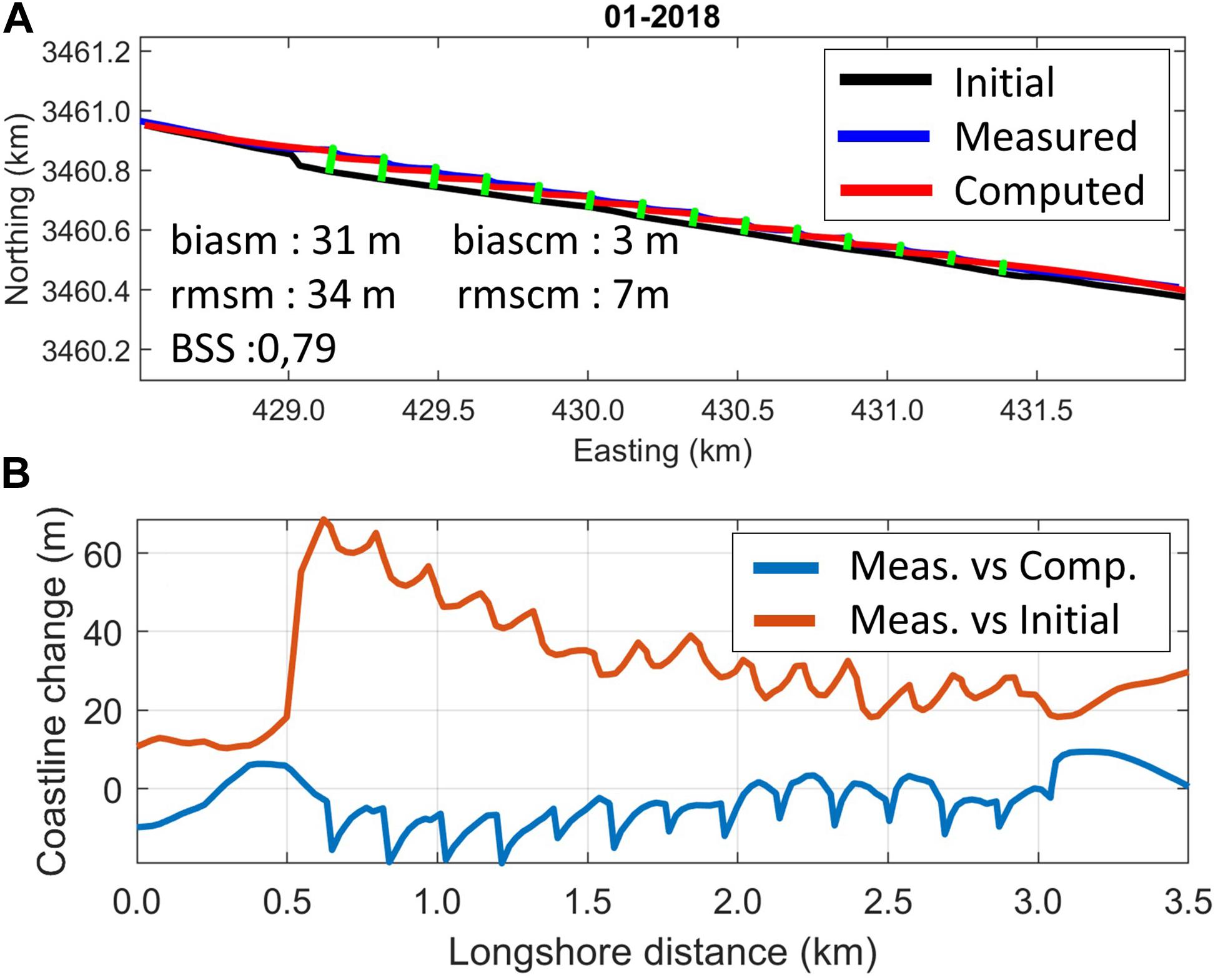
Figure 14. Measured (meas.) and computed (comp.) coastline evolution 2011-2018, Al-Gamil (A); observed change and difference between measurements and model results (B).
Figure 14 indicates that the model has produced satisfactory results compared to reality, although the diffraction phenomena behind the structures were not taken into account, leading to local errors just in the lee of each groin. The advancement of the coastline and the increase of the bypassing factor, BPF, were high during the first six months due to the high nourishment rates. Then, the nourishment was stopped and the coastline kept advancing due to the longshore transport and the bypassed sediment. Furthermore, the coastline reached a stable state at the tips of the groins where the maximum bypassing factor, BPF, was achieved, proving the validity of the model in representing the effect of bypassing in stabilizing the coastline.
Similar error statistics as for the Sand Engine case were computed, with a small bias and rms error of 3 m and 7 m, respectively, between measured values and model results, compared to rms of measured changes of 34 m. The model performed in the category excellent, with a BSS of 0.79.
Discussion
The flexible grid in the ShorelineS model allows for the evaluation of coastline changes for a wide range of applications that are not covered in most existing models, such as complex spit development and merging islands. At the same time, the standard cases with mildly curved coastlines are dealt with successfully. The model is extremely easy to run, as it merely requires initial coastline polylines, polylines of hard structures, offshore wave data and some parameter settings. These data are generally readily available through satellite imagery and global or regional wave hindcasts, or local wave data.
A first validation with a complex real-world case (the Sand Engine; de Schipper et al., 2016) shows that the methodology has the potential to be used as an efficient engineering tool, accurately reproducing the average erosion of the peninsula over time. The initial deformation of the spit and welding to the coast is impossible to simulate with standard coastline models, and the detailed 2DH morphodynamic models that can, in principle, describe this take several orders of magnitude more computation time (months vs. tens of minutes). Also the accretion on both sides of the harbor of IJmuiden, as described in Roelvink and Reniers (2011), is readily reproduced. Apparently, the shielding of waves at the structures is already sufficient to reproduce the local coastline orientation. The case of Al Gamil, Egypt also shows that the effect of local structures such as the groin scheme implemented there, in combination with nourishments, can be simulated with excellent skill, when a realistic bypassing function is applied.
The active profile depth is typically fixed in coastline models such as ShorelineS, but may, in practice, vary spatially and temporally depending on the wave conditions and the pre-existing bathymetry. The current approach is considered suitable for coastlines with rather uniform profiles (with similar orientation toward the sea), which is often the case for a shelf sea coast (e.g., in the Netherlands or Gulf countries). The Sand Engine case could, for example, be modeled well with just a single active height despite being a complex landform with slightly different conditions acting at the seaward extending head and lateral sides. However, the antecedent bathymetry may play a large role for landward propagating coastal barriers or spits over low-lying marshes or lagoons, where the seaward side is much more exposed to waves than the landward side, which is much shallower. Consequently, the landward retreat of spits due to overwash may be less than computed by the model, taking into account that less sand is needed on the landward side to build the profile. A more precise definition of the active heights based on global and local resources would, therefore, be very desirable for such situations to precisely assess these changes at landward propagating coastal barriers or spits over low-lying marshes or lagoons.
In sediment-starved nearshore regions, the actual alongshore sediment transport is smaller than the potential transport, which eventually affects the alongshore gradient and corresponding morphological change, as shown by Payo et al. (2018). In our model such processes are not yet represented.
An easy step to take into account variations in wave height and direction due to refraction over uneven offshore bathymetry is to create a transformation table from offshore to nearshore wave conditions along a depth contour or on a large-scale grid, from which ShorelineS can interpolate the alongshore-varying wave direction and height. Such applications are already applied in practice and ShorelineS supports this through the use of a fast 2D wave refraction solver. Steps further are to feed back the shoreline changes into the bathymetry used in the wave model, as e.g., in Robinet et al. (2018), or to even consider emerged, un-erodible layers due to geological formations, which may potentially be buried by sand but may have a significant influence on shoreline evolution, as in Robinet et al. (2020).
The flexible grid is essential for unconstrained modeling of strongly curved local coastline features such as salients and tombolos at offshore breakwater schemes. Many methods are available to estimate the effect of diffraction and refraction behind offshore breakwaters and other hard structures or headlands (Wiegel, 1962; Goda et al., 1978; Dabees, 2000), which can, in combination with the flexible grid of ShorelineS, be used to quickly and accurately evaluate the morphological development of salients or tombolos behind structures. This will be a great step forward since the existing reduced complexity coastline models on the other hand suffer from the requirement that a reference position of the grid should be provided (Hsu et al., 2010; Ruggiero and Buijsman, 2010) which cannot follow the considerable changes in coastline curvature that may take place when a tombolo develops. Even the complex field models solving these features on a map often need very dense grids or require rather elaborate wave modeling, such as Boussinesq wave modeling (Karambas and Samaras, 2014), thus slowing down simulations considerably. These models often have difficulties in assessing the precise position of the waterline as a natural profile shape is difficult to maintain (Grunnet et al., 2004; van Duin et al., 2004). First steps to include diffraction in ShorelineS were taken in Elghandour (2018) and full implementation and validation will be described in an upcoming paper.
The current approach used in the ShorelineS model assumes a static profile which can move in the cross-shore direction depending on incoming sand supply and the defined active height. In practice this works well for most engineering problems, which are dominated by the alongshore wave-driven transport and act at a yearly time scale. Over longer time-frames the smaller but consistently present cross-shore losses play an increasingly important role as was shown by Vitousek et al. (2017) for the erosion at the Pacific Coast of California. In their study they estimated that sea level rise will contribute 69% of the losses over the period 2010 to 2100, while it contributes only 1% over the hindcast period from 1995 to 2010. Approaches to account for sea-level rise (e.g., effect, barrier rollover and basin infilling) will be needed to further enhance the capabilities of ShorelineS on longer time horizons. In addition, it is considered relevant to also include seasonal changes due to wave energy variations (Yates et al., 2009) to keep track of a set of cross-shore profile positions (Larson et al., 2016). It will then be possible to also assess seasonal variations in beach position and potential retreat rates for extreme situations (Ranasinghe et al., 2012). Ensemble forecasts can then be made with the relatively swift ShorelineS model to assess a number of realizations of the future coastline position accounting for variations in initial and boundary conditions as well as uncertainty in model parameters. The potential for such approaches was recently shown by Montaño et al. (2020) in a unique comparison of a number of mostly equilibrium-type cross-shore models and data-driven models against a 15-year calibration dataset followed by a blind 3-year ‘shorecast.’
The relatively straightforward model input of the ShorelineS model provides a unique opportunity to automatically process large data sets of remotely sensed coastal information, as the precise definition of the coastal reference lines does not affect the forecasts. Satellite derived time-series of shoreline positions (Luijendijk et al., 2018) may be derived at intervals of days to a few months (depending on the number of cloudy days) with sub-pixel accuracy. This provides a basis for calibration and validation of coastline models, which continuously improve the predictions through data-assimilation.
Coastline models are typically not suitable for the details of the rather complex three-dimensional (3D) bathymetries in the vicinity of tidal inlets, but as an outlook to the future it is envisioned that 2DH bathymetry can be coupled to the ShorelineS model for which computations of tide and waves can be performed with a numerical model. A two-way coupling between the coastline and a relatively coarse hydraulic 2DH model such as Delft3D (Lesser et al., 2004), can already provide very accurate morphological computations solving the tidal currents, without the need of placing very detailed grid cells in the 2DH model as the transport processes close to the coast are solved within ShorelineS. Changes in coastline position feed back into the 2DH model bathymetry by assuming a cross-shore profile shape. Such developments are also considered essential for long-term computations of coastline development to assess the effects of climate change or geological reconstructions of coasts and deltas, since the computational power of present-day computers is hardly sufficient to solve the effects of longshore currents at large coastal sections (> 100 km) over yearly time scales. As such, the potential of ShorelineS to be easily coupled to more complex field models with relatively coarse grids is a necessity for answering future questions related to sea level rise at century time scales.
Another, much less cumbersome method to treat the behavior of river mouths and tidal inlets through simple algorithms that keep a mouth open at a specified width depending on the discharge, redistribute sediment locally or add the sediment discharge of the river to the adjacent coastal areas. Such approaches have recently been tested and will be the subject of upcoming papers.
Conclusion
The development of a new coastline model is described and the model was applied to a number of theoretical and field cases, showing the value of the application of a flexible grid. The test cases show that the model can represent the physics of both low and high-angle wave incidence coasts with simple structures. Quantitatively the model can accurately hindcast the erosion of a large-scale temporary land reclamation (Sand Engine), providing confidence that not only the patterns but also the spatial distribution of changes can be predicted, with only a single transport coefficient as a calibration parameter. The Brier Skill Score (BSS) increases with time from 0.22 shortly after construction to around 0.7 after a few years. A second validation case describing a groin scheme in Egypt show similar skill when an appropriate groin bypassing function is applied. As such the model is very capable of resolving coastline changes at intermediate time scales (years) for rather alongshore uniform coasts or coasts with spit features. Still, a number of relevant aspects could be improved that are likely to affect performance of the model at short (days to months) and long (decades to centuries) timescales, such as the inclusion of small but consistent losses due to sea level rise (e.g., profile adaptation and ingress of sediment in tidal basins) and a potential retreat due to storms for statistical analyses of coastal safety.
In general, a large number of coastal issues can be solved with the ShorelineS model thanks to the flexible grid, which will allow its application to coasts with large changes in shape such as present at local salient and tombolo developments. Even the migration of barrier islands and tidal inlets is expected to be possible in the near future when ShorelineS is coupled with relatively simple 2DH models (e.g., Delft3D, XBeach) that provide nearshore source/sink terms while ShorelineS updates the 2D bathymetric changes. Development is continuing on a number of issues as previously outlined.
Data Availability Statement
Publicly available datasets were analyzed in this study. This data can be found here: https://data.4tu.nl/repository/collection:zandmotor. Matlab source code for the ShorelineS model is available at www.shorelines.nl.
Author Contributions
DR developed the original code, carried out the principle tests, supervised AE and MG and is lead author. BH improved the code structure, implemented different transport formulations, developed the Sand Engine test case and contributed to the manuscript. AE carried out validation tests, solved a number of issues with the code and contributed to the manuscript writing. MG improved the treatment of groins and carried out the Al Gamil field test. JR co-supervised AE and MG and contributed to the model code and manuscript. All authors contributed to the article and approved the submitted version.
Funding
AE was funded by Portuguese Science Foundation (FCT) through project: ALG-01-0145-FEDER913 28949 “ENLACE”. BH contributed in the framework of Deltares Strategic Research.
Conflict of Interest
The authors declare that the research was conducted in the absence of any commercial or financial relationships that could be construed as a potential conflict of interest.
Supplementary Material
The Supplementary Material for this article can be found online at: https://www.frontiersin.org/articles/10.3389/fmars.2020.00535/full#supplementary-material
References
Antolínez, J. A. A., Méndez, F. J., Anderson, D., Ruggiero, P., and Kaminsky, G. M. (2019). Predicting climate-driven coastlines with a simple and efficient multiscale model. J. Geophys. Res. 124, 1596–1624. doi: 10.1029/2018JF004790
Arriaga, J., Rutten, J., Ribas, F., Falqués, A., and Ruessink, G. (2017). Modeling the long-term diffusion and feeding capability of a mega-nourishment. Coast. Eng. 121, 1–13. doi: 10.1016/J.COASTALENG.2016.11.011
Ashton, A. D., and Murray, A. B. (2006). High-angle wave instability and emergent shoreline shapes: 1. Modeling of sand waves, flying spits, and capes. J. Geophys. Res. Earth Surf. 111, 1–19. doi: 10.1029/2005JF000422
Ashton, A. D., Murray, A. B., and Arnoult, O. (2001). Formation of coastline features by large-scale instabilities induced by high-angle waves. Nature 414, 296–300. doi: 10.1038/415666a
Ashton, A. D., Nienhuis, J., and Ells, K. (2016). On a neck, on a spit: controls on the shape of free spits. Earth Surf. Dyn. 4, 193–210. doi: 10.5194/esurf-4-193-2016
Barbier, E. B., Hacker, S. D., Kennedy, C., Koch, E. W., Stier, A. C., and Silliman, B. R. (2011). The value of estuarine and coastal ecosystem services. Ecol. Monogr. 81, 169–193. doi: 10.1890/10-1510.1
Bijker, E. W. (1967). Some Considerations About Scales for Coastal Models with Movable Bed. Publication No. 50. Delft: Delft Hydraulics Laboratory.
Bruun, P. (1962). Sea level rise as a cause of shore erosion. J. Waterways Harb. Divis. 88, 117–132.
Dabees, M. (2000). Efficient Modeling of Beach Evolution. Ph.D. Thesis, Queen’s University, Kingston.
de Schipper, M. A., de Vries, S., Ruessink, G., de Zeeuw, R. C., Rutten, J., van Gelder-Maas, C., et al. (2016). Initial spreading of a mega feeder nourishment: observations of the Sand Engine pilot project. Coast. Eng. 111, 23–38. doi: 10.1016/J.COASTALENG.2015.10.011
Dean, R. G. (1991). Equilibrium beach profiles: characteristics and applications. J. Coast. Res. 7, 53–84.
Elfrink, B., Prestedge, G., Rocha, C. B. M., and Juhl, J. (2003). “Shoreline evolution due to highly oblique incident waves at Walvis Bay, Namibia,” in Proceeding International Conference on Coastal Sediments 2003, (Clearwater Beach, FL: U. S. World Scientific).
Elghandour, A. M. (2018). Efficient Modelling of coastal evolution Development, verification and validation of ShorelineS Model. Delft: IHE Delft Insitute for Water Education.
Falqués, A., and Calvete, D. (2005). Large-scale dynamics of sandy coastlines: diffusivity and instability. J. Geophys. Res. Oceans 110, 1–15. doi: 10.1029/2004JC002587
Falqués, A., Ribas, F., Idier, D., and Arriaga, J. (2017). Formation mechanisms for self-organized kilometer-scale shoreline sand waves. J. Geophys. Res. Earth Surf. 122, 1121–1138. doi: 10.1002/2016JF003964
Ghonim, M. E. (2019). Recent Developments in Numerical Modelling of Coastline Evolution Advanced Development and Evaluation of ShorelineS Coastline Model. Delft: IHE Delft Institute for Water Education.
Goda, Y., Takayama, T., and Suzuki, Y. (1978). “Diffraction diagrams for directional random waves,” in Proceedings of the Coastal Engineering 1978 (New York, NY: American Society of Civil Engineers), 628–650.
Grunnet, N. M., Walstra, D.-J. R., and Ruessink, B. G. (2004). Process-based modelling of a shoreface nourishment. Coast. Eng. 51, 581–607. doi: 10.1016/J.COASTALENG.2004.07.016
Hanson, H., and Kraus, N. C. (2011). Long-term evolution of a long-term evolution model. J. Coast. Res. 59, 118–129. doi: 10.2112/SI59-012.1
Hsu, J. R.-C., Yu, M.-J., Lee, F.-C., and Benedet, L. (2010). Static bay beach concept for scientists and engineers: a review. Coast. Eng. 57, 76–91. doi: 10.1016/J.COASTALENG.2009.09.004
Huisman, B. J. A., Ruessink, B. G., de Schipper, M. A., Luijendijk, A. P., and Stive, M. J. F. (2018). Modelling of bed sediment composition changes at the lower shoreface of the Sand Motor. Coast. Eng. 132, 33–49. doi: 10.1016/J.COASTALENG.2017.11.007
Hurst, M. D., Barkwith, A., Ellis, M. A., Thomas, C. W., and Murray, A. B. (2015). Exploring the sensitivities of crenulate bay shorelines to wave climates using a new vector-based one-line model. J. Geophys. Res. F Earth Surf. 120, 2586–2608. doi: 10.1002/2015JF003704
Idier, D., Falqués, A., Ruessink, B. G., and Garnier, R. (2011). Shoreline instability under low-angle wave incidence. J. Geophys. Res. Earth Surf. 116:F04031. doi: 10.1029/2010JF001894
Kaergaard, K., and Fredsoe, J. (2013a). A numerical shoreline model for shorelines with large curvature. Coast. Eng. 74, 19–32. doi: 10.1016/j.coastaleng.2012.11.011
Kaergaard, K., and Fredsoe, J. (2013b). Numerical modeling of shoreline undulations part 2: varying wave climate and comparison with observations. Coast. Eng. 75, 77–90. doi: 10.1016/j.coastaleng.2012.11.003
Kamphuis, J. W. (1991). Alongshore sediment transport rate. J. Waterway PortCoast. Ocean Eng. 117, 624–640. doi: 10.1061/(asce)0733-950x(1991)117:6(624)
Karambas, T. V., and Samaras, A. G. (2014). Soft shore protection methods: the use of advanced numerical models in the evaluation of beach nourishment. Ocean Eng. 92, 129–136. doi: 10.1016/J.OCEANENG.2014.09.043
Kristensen, S. E., Drønen, N., Deigaard, R., and Fredsoe, J. (2016). Impact of groyne fields on the littoral drift: a hybrid morphological modelling study. Coast. Eng. 111, 13–22. doi: 10.1016/j.coastaleng.2016.01.009
Larson, M., Hanson, H., and Kraus, N. C. (1987). Analytical Solutions of the On-line Model of Shoreline Change. Reston: ASCE.
Larson, M., Hanson, H., and Kraus, N. C. (1997). Analytical solutions of one-line model for shoreline change near coastal structures. J. Waterway Port Coast. Ocean Eng. 123, 180–191. doi: 10.1061/(asce)0733-950x(1997)123:4(180)
Larson, M., Palalane, J., Fredriksson, C., and Hanson, H. (2016). Simulating cross-shore material exchange at decadal scale. Theory and model component validation. Coast. Eng. 116, 57–66. doi: 10.1016/J.COASTALENG.2016.05.009
Leatherman, S. P. (1979). Migration of Assateague Island, Maryland, by inlet and overwash processes. Geology 7, 104–107.
Lesser, G. R., Roelvink, J. A., van Kester, J. A. T. M., and Stelling, G. S. (2004). Development and validation of a three-dimensional morphological model. Coast. Eng. 51, 883–915. doi: 10.1016/j.coastaleng.2004.07.014
Luijendijk, A. P., Hagenaars, G., Ranasinghe, R., Baart, F., Donchyts, G., and Aarninkhof, S. (2018). The state of the world’s beaches. Sci. Rep. 8:6641. doi: 10.1038/s41598-018-24630-6
Luijendijk, A. P., Ranasinghe, R., de Schipper, M. A., Huisman, B. A., Swinkels, C. M., Walstra, D. J. R., et al. (2017). The initial morphological response of the Sand Engine: a process-based modelling study. Coast. Eng. 119, 1–14. doi: 10.1016/J.COASTALENG.2016.09.005
Montaño, J., Coco, G., Antolínez, J. A. A., Beuzen, T., Bryan, K. R., Cagigal, L., et al. (2020). Blind testing of shoreline evolution models. Sci. Rep. 10, 1–10. doi: 10.1038/s41598-020-59018-y
Palalane, J., and Larson, M. (2020). A long-term coastal evolution model with longshore and cross-shore transport. J. Coast. Res. 36, 411–423. doi: 10.2112/JCOASTRES-D-17-00020.1
Payo, A., Favis-Mortlock, D., Dickson, M., Hall, J. W., Hurst, M. D., Walkden, M. J. A., et al. (2017). Coastal Modelling Environment version 1.0: a framework for integrating landform-specific component models in order to simulate decadal to centennial morphological changes on complex coasts. Geosci. Model Dev. 10, 2715–2740. doi: 10.5194/gmd-10-2715-2017
Payo, A., Walkden, M., Ellis, M. A., Barkwith, A., Favis-Mortlock, D., Kessler, H., et al. (2018). A quantitative assessment of the annual contribution of platform downwearing to beach sediment budget: Happisburgh, England, UK. J. Mar. Sci. Eng. 6:113. doi: 10.3390/jmse6040113
Pelnard-Considère, R. (1956). Essai de theorie de l’evolution des formes de rivage en plages de sable et de galets. Les Energies de La Mer 1, 13–15.
Ranasinghe, R., Callaghan, D., and Stive, M. J. F. (2012). Estimating coastal recession due to sea level rise: beyond the Bruun rule. Clim. Change 110, 561–574. doi: 10.1007/s10584-011-0107-8
Ranasinghe, R., Duong, T. M., Uhlenbrook, S., Roelvink, D., and Stive, M. (2013). Climate-change impact assessment for inlet-interrupted coastlines. Nat. Clim. Change 3, 83–87. doi: 10.1038/nclimate1664
Robinet, A., Castelle, B., Idier, D., Harley, M. D., and Splinter, K. D. (2020). Controls of local geology and cross-shore/longshore processes on embayed beach shoreline variability. Mar. Geol. 422:106118. doi: 10.1016/j.margeo.2020.106118
Robinet, A., Idier, D., Castelle, B., and Marieu, V. (2018). A reduced-complexity shoreline change model combining longshore and cross-shore processes: the LX-Shore model. Environ. Model. Softw. 109, 1–16. doi: 10.1016/j.envsoft.2018.08.010
Roelvink, D., and Reniers, A. (2011). A Guide to Modeling Coastal Morphology. Singapore: World Scientific.
Ruggiero, P., and Buijsman, M. (2010). Modeling the effects of wave climate and sediment supply variability on large-scale shoreline change. Mar. Geol. 273, 127–140. doi: 10.1016/J.MARGEO.2010.02.008
Stive, M. J. F., de Schipper, F., Matthieu, A., Luijendijk, A. P., Aarninkhof, S. G. J., van Gelder-Maas, C., et al. (2013). A new alternative to saving our beaches from sea-level rise: the sand engine. J. Coast. Res. 29, 1001–1008. doi: 10.2112/JCOASTRES-D-13-00070.1
Sutherland, J., Peet, A. H., and Soulsby, R. L. (2004). Evaluating the performance of morphological models. Coast. Eng. 51, 917–939. doi: 10.1016/j.coastaleng.2004.07.015
Syvitski, J. P. M., Vörösmarty, C. J., Kettner, A. J., and Green, P. (2005). Impact of humans on the flux of terrestrial sediment to the global coastal ocean. Science 308, 376–380. doi: 10.1126/science.1109454
Tonnon, P. K., Huisman, B. J. A., Stam, G. N., and van Rijn, L. C. (2018). Numerical modelling of erosion rates, life span and maintenance volumes of mega nourishments. Coast. Eng. 131, 51–69. doi: 10.1016/J.COASTALENG.2017.10.001
Tran, Y. H., and Barthélemy, E. (2020). Combined longshore and cross-shore shoreline model for closed embayed beaches. Coast. Eng. 158:103692. doi: 10.1016/j.coastaleng.2020.103692
USACE (1984). Shore Protection Manual. Coastal Engineering Research Center (Vol. 1). Washington, DC: US Army Corps of Engineers.
van den Berg, N., Falqués, A., and Ribas, F. (2011). Long-term evolution of nourished beaches under high angle wave conditions. J. Mar. Syst. 88, 102–112. doi: 10.1016/J.JMARSYS.2011.02.018
van Duin, M. J. P., Wiersma, N. R., Walstra, D. J. R., van Rijn, L. C., and Stive, M. J. F. (2004). Nourishing the shoreface: observations and hindcasting of the Egmond case, The Netherlands. Coast. Eng. 51, 813–837. doi: 10.1016/J.COASTALENG.2004.07.011
van Rijn, L. C. (2014). A simple general expression for longshore transport of sand, gravel and shingle. Coast. Eng. 90, 23–39. doi: 10.1016/j.coastaleng.2014.04.008
Vitousek, S., and Barnard, P. L. (2015). “A nonlinear, implicit one-line model to predict long-term shoreline change,” in Proceedings of the Coastal Sediments 2015, (Singapore: World Scientific).
Vitousek, S., Barnard, P. L., Limber, P., Erikson, L., and Cole, B. (2017). A model integrating longshore and cross-shore processes for predicting long-term shoreline response to climate change. J. Geophys. Res. Earth Surf. 122, 782–806. doi: 10.1002/2016JF004065
Wiegel, R. L. (1962). Diffraction of waves by semi-infinite breakwater. J. Hydraulics Divis. ASCE 88, 27–44.
Keywords: coastal evolution, coastline model, spit, barrier, salient, tombolo
Citation: Roelvink D, Huisman B, Elghandour A, Ghonim M and Reyns J (2020) Efficient Modeling of Complex Sandy Coastal Evolution at Monthly to Century Time Scales. Front. Mar. Sci. 7:535. doi: 10.3389/fmars.2020.00535
Received: 20 March 2020; Accepted: 12 June 2020;
Published: 03 July 2020.
Edited by:
Rafael Almar, Institut de Recherche Pour le Développement (IRD), FranceReviewed by:
Andrés Payo, British Geological Survey (BGS), United KingdomBruno Castelle, Centre National de la Recherche Scientifique (CNRS), France
Copyright © 2020 Roelvink, Huisman, Elghandour, Ghonim and Reyns. This is an open-access article distributed under the terms of the Creative Commons Attribution License (CC BY). The use, distribution or reproduction in other forums is permitted, provided the original author(s) and the copyright owner(s) are credited and that the original publication in this journal is cited, in accordance with accepted academic practice. No use, distribution or reproduction is permitted which does not comply with these terms.
*Correspondence: Dano Roelvink, ZC5yb2Vsdmlua0B1bi1paGUub3Jn