Biophysical Control on Variability in Phytoplankton Production and Composition in the South-Western Tropical Indian Ocean During Monsoon 2014

The existing oligotrophic conditions in the southwest tropical Indian Ocean (SWTIO) is believed to be one of the causes for low phytoplankton productivity (PP) observed in this area. Though many remote sensing based studies on PP have been carried out in SWTIO, studies on in situ estimation of PP and its cause(s) of variability are scarce. Thus, to understand the controlling environmental forcings on the variability in phytoplankton biomass (chlorophyll-a; Chl-a), community structure and productivity, time series (TS; @6 h intervals for 10 days; 1 station), plus point measurements (RT; 3 stations) were carried out in the SWTIO during the southwest monsoon (June) of 2014. Strong thermohaline stratification resulted in shallow (35–40 m) mixed layer (ML). Subsurface Chl-a maximum (SCM) was observed to oscillate within 40–60 m with majority of peaks at ∼50 m, and existed just beneath the ML depth. Light availability during sampling period was highly conducive for algal growth; nutrient ratios indicated N- and Si-limitation (N:P < 10; N:Si < 1 and SiO₄ < 5 μM) suggesting unfavorable conditions for diatoms and/or silicoflagellates growth within the ML. Furthermore, HPLC-based pigments analysis confirmed dominance of nano-sized plankton (53%) followed by pico-plankton (25%) and micro-plankton (22%). Column integrated production (IPP) varied from 176 to 268 (241 ± 43 mgC m^–2 d^–1) and was relatively stable during the observation period, except a low value (19.4 E m^–2 d^–1) on 11 June, which was ascribed to the drastic dropdown in the daily incident PAR due to overcast sky. Vertical profiles of PP and Chl-a resembled each other and maximum PP usually corresponded with SCM depths. The Chl-a-specific PP (P^B) was mostly higher within the ML and showed no surface photoinhibition, due to the dominance of smaller phytoplankton (less prone to pigment packaging effect) in the surface layer. Comparatively, higher P^B within the ML is indicative of phytoplankton healthiness during the sampling time, whereas low P^B below the SCM was due to light limitation. Highest integrated Chl-a (39 mg m^–2) and IPP (328 mgC m^–2 d^–1) observed at RT-2 was clearly linked to low sea surface height anomaly (SSHA), cyclonic disturbance, and associated positive Ekman suction. Conversely, high SSHA and strong stratification conditions prevailed at TS, RT-4, and RT-6 stations leading to comparatively lower IPP (176-268, 252, and 243 mgC m^–2 d^–1), respectively.

Introduction

Oceanic phytoplankton, being the base of marine food-web, plays a crucial role in global biogeochemical cycles (Falkowski et al., 1994), regulates the global climate (Sabine et al., 2004), fisheries (Stock et al., 2017), and the condition and variability of life in the oceans. Understanding alterations in global ocean phytoplankton production (PP) is one of the pressing issues in ocean biogeochemistry because it not only provides vital insights to the bio−physical interactions of the ecosystem (Naqvi et al., 2010) but also offer biophysical feedbacks (Murtugudde et al., 1999). Through the process of PP significant drawdown of atmospheric CO₂ occurs which is subsequently transported to the ocean interior through “biological pump” (Longhurst and Harrison, 1989). Thus, it is essential to gain clear perception of the cause(s) responsible for PP variability in the oceanic environment. Basically, PP is a function of four variables viz., photosynthetically active radiation (PAR), nutrients, phytoplankton biomass (chlorophyll-a), and water temperature (Behrenfeld and Falkowski, 1997b), and hence any adverse changes in the above variables can have telling effect on PP variability which would cascade through the entire food-web in the region.

The southwest tropical Indian Ocean (SWTIO) situated between 5°S to 10°S and 50°E to 80°E is one of the major upwelling area in the Indian Ocean region due to the presence of Seychelles–Chagos Thermocline Ridge (SCTR) system characterized by a thermocline shallower than the euphotic zone (Murtugudde and Busalacchi, 1999; Wiggert et al., 2005). The SWTIO is influenced by the unique seasonally reversing monsoon wind systems that act as the major physical driver for the prevailing upwelling processes resulting in significant variability in sea surface temperature (SST) in different timescales, in comparison to the other regions of Indian Ocean (Annamalai et al., 2003; Zhou et al., 2008; Jung and Kirtman, 2016). Also, rising SST in this region can enhance surface stratification inhibiting vertical mixing, thereby dwindling supply of nutrients into the well-lit euphotic zone where photosynthesis takes place (Behrenfeld et al., 2006; Roxy et al., 2016). Fluctuations in the vertical mixing process also influences the overall time span of light experienced by the phytoplankton (McCreary et al., 1996) in the water column. Moreover, the variability in bio-physical processes in SWTIO region are mostly controlled by the strength and duration of the monsoon winds and associated nutrient dynamics, and the downward trend in biological production, if any, in these upwelling systems has immense ramification on the marine food-web and economic status of the fishing community of this region (Roxy et al., 2016; Sreeush et al., 2018).

The SWTIO region is climatologically and biologically important because of active upwelling processes and/or the shallow thermocline, which is prone to the atmospheric forcing at different time scales (Wiggert et al., 2006). The vertical turbulence effectively exchanges heat with the thermocline, introducing cooler thermocline waters to the surface. Nevertheless, SST in the SWTIO is much warmer (annual mean is 28°C) than the surface waters from other upwelling tropical regions like eastern equatorial Pacific Ocean and Atlantic Ocean (George et al., 2013). In Northwest Indian Ocean (Arabian Sea) frequent occurrence of phytoplankton blooms was reported (Prasanna Kumar et al., 2001; Wiggert et al., 2005; Naqvi et al., 2010), which was attributed to the strong monsoonal wind forcing in this region that lead to year-round upwelling resultant from coastal divergence of Ekman transport and from Ekman suction (Murtugudde et al., 1996), replenishing nutrients in the surface and supporting higher rates of PP (Wiggert et al., 2005; McCreary et al., 2009; Resplandy et al., 2011). On the other hand, the surface phytoplankton blooms observed in the oligotrophic SCTR region is caused by nutrients entrainment into the mixed layer (ML) and/or the dispersal of phytoplankton from the deep chlorophyll maximum (DCM) layer to the surface layer (Resplandy et al., 2009). Furthermore, Resplandy et al. (2009) opined that SCTR region is typified by local Ekman suction-induced Open Ocean upwelling, which sustains shallow ML throughout the year, and hence responsive to atmospheric forcing. Furthermore, studies have shown that the propagation of internally generated Rossby waves modifies the depth of the thermocline and thus influences the PP because the thermocline is shallower than the euphotic zone in this region (Wiggert et al., 2006, 2009).

George et al. (2013) studied the physical control of the chlorophyll-a distribution during winter and summer monsoon and opined that surface freshening controls the chlorophyll-a by modulating static stability and ML depth. Ocean warming induced an alarming decline of up to 20% in phytoplankton over the past 60 years (Roxy et al., 2016), and impact of the Indian Ocean Dipole (IOD) and El Niño Southern Oscillation (ENSO) on significant interannual variation chlorophyll-a has been reported (Dilmahamod et al., 2016) in this region. Resplandy et al. (2009) have shown that interannual variability of the thermocline and its role modulating the response to Madden-Julian Oscillation (MJO) controls the chlorophyll-a and export flux of carbon. Further, recent study has shown that Ocean Carbon-Cycle Model Intercomparison Project (OCMIP-II)–based estimated CO₂ flux and pCO₂ underestimated the SCTR variability portraying it as a CO₂ sink region (Sreeush et al., 2018). Studies carried out in the SCTR region either describe the role of physical forcings in modulating the phytoplankton biomass (chlorophyll-a) concentrations (George et al., 2013; Roxy et al., 2016; Dilmahamod et al., 2016) and/or satellite or model-based PP (Resplandy et al., 2009; Sreeush et al., 2018); however, none of the studies have reported any in situ measured phytoplankton C-uptake rates (PP), phytoplankton size class/community, and phytoplankton physiological perspective vis-à-vis the physical forcings prevailing in this oligotrophic region. Hence, this study investigates the spatiotemporal variability in sea truth PP and phytoplankton composition with respect to the prevailing environmental forcings. To the best of our comprehension, this is the first report of in situ measurements of PP and phytoplankton size class/community from this area, which would enhance our understanding of the existing bio−physical interactions and plug our knowledge gaps.

Materials and Methods

Study Area, Sampling Periodicity, and Hydrography

Part of the study area (Figure 1) is located in the Seychelles-Chagos Thermocline Ridge (SCTR, 5°S–10°S, 50°E–80°E) in the southwest tropical Indian Ocean (SWTIO) as defined by Hermes and Reason (2008) and part in the equatorial Indian Ocean (EIO) region. Year-round occurrence of upwelling phenomena is one of the salient features of SCTR region (Woodberry et al., 1989; McCreary et al., 1993), nevertheless oligotrophic conditions prevails in this area. Existence of Ekman suction driven upwelling (Spencer et al., 2005) and shallow thermocline signifies this region’s importance in the perspective of biological productivity. Due to shallow thermocline the influence of physical forcings on phytoplankton bloom/productivity in this region is clearly discernible (Wiggert et al., 2006, 2009; Resplandy et al., 2009; George et al., 2013).

FIGURE 1

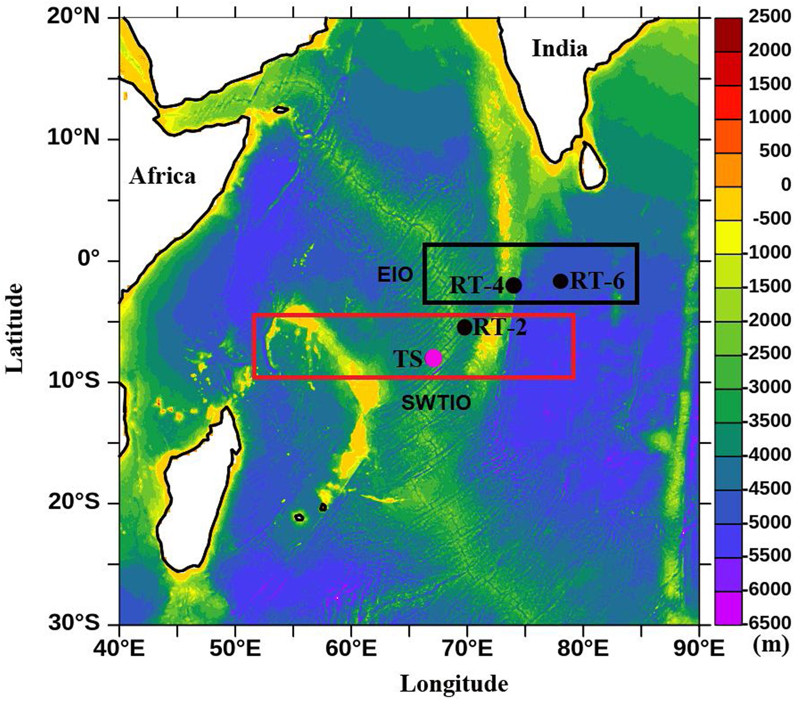
Figure 1. Study area map showing the four sampling locations. The black and pink dots indicate return track (RT) and time series (TS) stations; red and black rectangle denotes the southwest tropical Indian Ocean (SWTIO) and equatorial Indian Ocean (EIO) region, respectively. Background colors indicate the bathymetry derived from ETOPO data.

Sampling was conducted onboard ORV-Sagar Nidhi at four stations in the study area during the monsoon season (June 9–23) of 2014. Time series (TS) observations (6-hourly interval over 10 days) were conducted at 08°S and 67°E; on the return track (RT) three discrete stations (RT-2 at 5.58^oS and 69.75^oE, RT-4 at 1.90^oS and 73.88^oE, and RT-6 at 1.73^oS and 77.97^oE) were also sampled (Table 1) for assessing same sets of parameters as carried out for TS station. Based on the geographical locations, the TS and RT-2 stations were considered as SCTR stations, whereas RT-4 and RT-6 were considered as the stations located in the EIO region.

TABLE 1

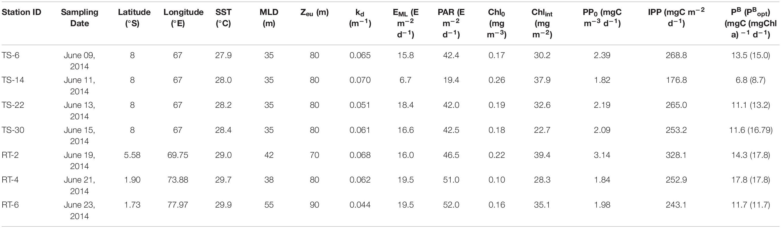
Table 1. Primary productivity and associated variables at sampling station: sea surface temperature (SST), mixed layer depth (MLD), euphotic depth (Z_eu), Vertical light attenuation coefficient (k_d), mean photosynthetically active radiation (PAR) level in the mixed layer (E_ML), daily surface PAR, surface chlorophyll-a (Chl₀), column-integrated chlorophyll-a (Chl_int), surface primary productivity (PP₀), column-integrated PP (IPP), surface Chl-a-specific PP (P^B), and maximum P^B in the water column (P^B_opt, in parenthesis).

The conductivity-temperature-depth (CTD) profiling were conducted using Sea-Bird (SBE-9plus, United States) instrumentation mounted on a Sea-Bird carousel, and the measured vertical profiles were used to determine the water mass properties of the study area. The CTD casts were performed at 6-hourly intervals at the TS station. Salinity measured by the CTD were calibrated against the values obtained from onboard Salinometer (Guildline 8400A). Sea surface temperature (SST) was recorded using a bucket thermometer (Theodor Friedrichs & Co.) with an accuracy of ± 0.2°C. Mixed layer depth (MLD) was determined based on a density (σ_t) change of 0.05 kg m^–3 at depth compared to near-surface. Water sampling from standard depths (0, 10, 20, 30, 50, 75, 100, 120, 150, and 200 m) were carried out by 5 L Niskin bottles (General Oceanics) attached to the carousel sampler.

Phytoplankton Pigments, Light, and Nutrients

Concentration of phytoplankton biomass (Chl-a; mg m^–3) was estimated by filtering 3 L of water samples onto 47 mm GF/F filters (Whatman^®) under dim light and low suction pressure (<0.1 kPa). The filters were kept frozen at −80°C till further analysis. Quantification of the pigments was carried out fluorometrically (10-AU, Turner Designs, United States) following overnight extraction of the GF/F filters in 10 ml of AR grade 90% acetone in dark and cool condition (Strickland and Parsons, 1972). Chl-a values at discrete depths were integrated to obtain column Chl-a (Chl_int; mg m^–2). Furthermore, 3 L of surface water samples at time series (TS) stations were filtered through 2 and 10 μm isopore-membrane filters (47 mm, Merck Millipore) and assayed fluorometrically (as described above) to estimate size-fractionated Chl-a contribution by smaller and larger phytoplankton size-classes. Due to logistical limitations we restricted the size-fractionation exercise to the above two size classes to approximate the % contribution by small (<2–10 μm) and large (>10 μm) phytoplankton. The above size-fractionation would not account for the picoplankton, and may not give appropriate estimation of the largest fraction (microplankton > 20 μm).

For phytoplankton pigments, 4 L of waters samples were filtered onto 25 mm GF/F filters and the filters were stored at −80°C till further analysis. Pigments analysis was also carried out by high-performance liquid chromatography (HPLC, Agilent Technologies) by means of XDB C8 column. Pigments separation was done by a binary solvent (solvent A-70/30: methanol/0.5M ammonium acetate; solvent B-100% methanol) gradient according to Kurian et al. (2012). Commercially available standards procured from DHI Inc. (Denmark) were used for the identification and quantification of pigments. In general, HPLC allows determining a suite of pigments (usually up to 15). In this study we identified seven pigments (i.e., Fucoxanthin, Peridinin, Alloxanthin, 19’-Hexanoyloxyfucoxanthin [19’HF], 19’-Butanoyloxyfucoxanthin [19’BF], Zeaxanthin, and TChl-b [Chl-b + divinyl chlorophyll-b]) as markers or diagnostic pigments (DP) of phytoplankton taxa as described in Uitz et al. (2006) to construct the “pigment indices” with objective to quantify phytoplankton taxonomic composition (%) with minimum number of pigments. The DP represents the sum of all the seven DP concentrations. Size-fractionated contributions of phytoplankton (f_micro [>20 μm], f_nano [2–20 μm], f_pico [<2 μm]) were calculated using following equations:

$$f_{micro}\%=$$

$$100\times (1.41[\mathrm{fucoxanthin}]+1.41[\mathrm{peridinin}])/\mathrm{\Sigma }DP(1)$$

$$f_{nano}\%=100\times (0.60[\mathrm{alloxanthin}]$$

$$+0.35[{19}^{\prime }\mathrm{BF}]+1.27[{19}^{\prime }\mathrm{HF}])/\mathrm{\Sigma }\mathrm{DP}(2)$$

$$f_{pico}\%=100$$

$$\times (0.86[\mathrm{zeaxanthin}]+1.01[\mathrm{TChlb}])/\mathrm{\Sigma }\mathrm{DP}(3)$$

Photosynthetically active radiation (PAR, 400–700 nm) at sea surface (E₀, m^–2 s^–1) was measured using a scalar irradiance sensor attached to the automatic weather station (AWS) mounted on the ship. The instantaneous values were integrated over the day length (dawn to dusk) to quantify daily incoming PAR (D_PAR; E m^–2 d^–1). Subsurface (E_z) PAR intensity were measured by a sensor (QSP-2200, Biospherical Inc.) attached to the CTD carousel, and the diffuse attenuation coefficient for downwelling PAR (k_d) was calculated according to Kirk (1994) as follows:

$$k_d=\frac{\ln ({\mathrm{E}}_0)-\ln ({\mathrm{E}}_{\text{z}})}{\text{z}}(4)$$

The euphotic depth, Z_eu (physical depth receiving 1% of E₀), was calculated as:

$${\text{Z}}_{eu}=\frac{1}{{\text{k}}_{\text{d}}}\times \text{ln}(100)(5)$$

by substituting k_d in the Beer-Lambert equation (Kirk, 1994). Mean light levels in the mixed layer (E_ML) at different stations were calculated as: E_ML = D_PAR[1-exp(-k_d.z)]/k_d.z (Boyd et al., 2007; Cheah et al., 2013), where z is the depth of the mixed layer. Water samples collected in pre-cleaned polypropylene bottles used for estimating concentrations of the inorganic macronutrients (NO₃, SiO₄, and PO₄) were determined onboard by a continuous flow autoanalyser (SKALAR Inc.).

Primary Productivity Measurements

Apart from the three discrete stations, primary productivity (PP) was also quantified every alternative day between 9 and 17 June 2014 at the time series station (Table 1). Water samples (3 L) were collected from five discrete depths corresponding to 100, 50, 25, 10, and 1% of surface irradiance. Samples were sieved through a 200 μm plankton mesh to exclude zooplankton grazers. After adding 1 ml of ¹⁴C [NaH¹⁴CO₃] in each sample (5 μCi per 250 ml of seawater in Nalgene bottles), the samples (in duplicates) were incubated in an on-deck incubation tank for 12 h (dawn to dusk) following standard simulated in situ incubation technique (UNESCO-JGOFS, 1994). To achieve the most realistic condition with regard to light quality and temperature during the incubations, the incubation tank temperature was maintained by continuously circulating surface seawater through the incubation tank. One bottle was immediately filtered for a time zero control (initial value), whereas two light and one dark bottle from each depth were incubated using appropriate density filters packets to compensate for light intensity (50, 25, 10, and 1%) for respective depths. Incubation was terminated by filtration of samples onto pre-combusted 25 mm GF/F filters (Whatman^®), followed by exposing them to concentrated HCl fumes to remove excess inorganic carbon. The filters were placed in scintillation vials and stored at −20°C until further analysis at shore laboratory. The activity was counted on a liquid scintillation counter (Packard 2500 TR) after adding 10 ml of scintillation cocktail (Lohrenz et al., 1992). Disintegrations per minute (dpm) were converted into daily PP (mgC m^–3 d^–1) at discrete depths (UNESCO-JGOFS, 1994) and the euphotic zone-integrated PP (IPP; mg C m^–2 d^–1) was estimated by trapezoidal integration. Chl-a-specific PP, (P^B; mgC [mgChl-a]^–1 d^–1) was calculated by normalizing PP with corresponding Chl-a. The optimum value of P^B in the water column was considered as P^B_opt.

The link between P^B and corresponding PAR in the water column (hereafter, PAR-P^B relationship) was established by curve-fitting. Here, the PAR-P^B relationship does not represent the true photosynthesis-irradiance (P-E) response of the same phytoplankton assemblages; rather, it symbolizes the association between the P^B and the corresponding PAR at discrete depths as described by Sakshaug et al. (1997). For curve fitting, P-E model (Webb et al., 1974) containing only two photosynthetic parameters was used, which can be described by the following equation:

$$P^B=P_{opt}^B\left[1-exp\left(-E/E_{max}\right)\right](6)$$

where P^B, P^B_opt, E_max are Chl a-normalized PP (mgC [mgChl-a]^–1 d^–1), Chl a-normalized optimal PP (mgC [mgChl-a]^–1 d^–1) in the water column, irradiance value at the point of inflection between light-limited and light-saturated phases (μE m^–2 d^–1), respectively. Since no photoinhibition was apparent, the above model was chosen for the dataset.

Primary Production Model

The vertically generalized production model (VGPM) proposed by Behrenfeld and Falkowski (1997a) was employed to estimate IPP from the satellite measured variables. This is a depth-integrated model, which relates sea surface Chl-a concentration (Chl₀) to Z_eu-integrated primary productivity (IPP) and can be expressed as:

$$IPP=\mathrm{\hspace{0.33em}0.66125}\times P_{opt}^B\times \left[\frac{E_0}{\left(E_0+4.1\right)}\right]\times Z_{eu}\times Ch{l}_0\times DL(7)$$

where IPP, P^B_opt, E₀, Z_eu, Chl₀, and DL are Z_eu-integrated daily PP (mgC m^–2 d^–1), Chl-a-normalized maximum PP in the vertical profile (mgC [mgChl-a]^–1 h^–1), PAR at sea surface (E m^–2 d^–1), depth (m) of the euphotic zone estimated from Chl₀ according to Morel and Berthon (1989), sea surface Chl-a (mg m^–3), and day-length (h) calculated as proposed by Kirk (1994), respectively. The light-dependent function [E₀/(E₀ + 4.1)] describes the relative change in the quantum efficiency of depth-integrated PP as a function of E₀; whereas as 0.66125 is a combined scaling factor for Chl-a concentration at discrete depth, and relative vertical distribution of C-fixation as a function of optical depth (Behrenfeld and Falkowski, 1997a). The P^B_opt, a photo-adaptive parameter necessary to convert the estimated biomass into photosynthetic rate, can be expressed as a 7^th order polynomial function of SST as described in Behrenfeld and Falkowski (1997a). Sea surface variables (i.e., SST, Chl₀, and E₀) were derived from Moderate Resolution Imaging Spectroradiometer (MODIS) and used as input for the VGPM to measure satellite estimates of IPP in the study area.

Satellite-Based Observations

Weekly average level-3 chlorophyll was derived from MODIS-Aqua for May and June 2014, whereas daily surface winds were derived from the Advanced Scatterometer (ASCAT). Daily SST was derived from Advanced Very High Resolution Radiometer (AVHRR) and daily sea surface height anomaly (SSHA) information was obtained from the Copernicus Marine Environment Monitoring Service (CMEMS) for the study period. Ekman suction velocity (W_e) was calculated using the equation:

$$W_e=\text{Curl}(\mathrm{\tau }/\mathrm{\rho }f)(8)$$

where τ, ρ, and f is the surface wind stress, density of the seawater, and Coriolis parameter, respectively.

Results

Hydrographic Variations Observed From CTD Profiling

At time series (TS) station the sea surface temperature (SST) ranged from 27.9–28.4°C (Table 1), whereas vertical variation of temperature laid between 12.0–28.17 (19.52 ± 5.26°C) with minimal variations in the upper 35–40 m compared to the deeper layers, and depicted a shallow thermocline (Figure 2A). Depth profile variation of salinity ranged from 34.38–35.31 (34.96 ± 0.20). Compared to temperature, variation of salinity was more prominent in the upper layer (Figure 2B). Occurrence of low saline and warm water mass formed a stratified surface layer and restricted the mixed layer depth (MLD) to 35–40 m as evidenced from the vertical profiles of sigma-t (Figure 2C) which varied between 21.97–27.42 (25.18 ± 1.77 kg m^–3-1000). Fluorescence profiles indicated clear subsurface Chl-a maximum (SCM) oscillating within 40–60 m with majority of peaks at ∼50 m, and existed just beneath the MLD (Figure 2D). The depth of the euphotic zone (Z_eu) was ∼80 m (Table 1) and did not vary over the study period. Z_eu was deeper than MLD resulting in moderately high Z_eu-MLD values (>35 m), implying that light availability during the sampling period was extremely favorable for algal growth within the ML (Sakshaug and Holm-Hansen, 1986; Westwood et al., 2011).

FIGURE 2

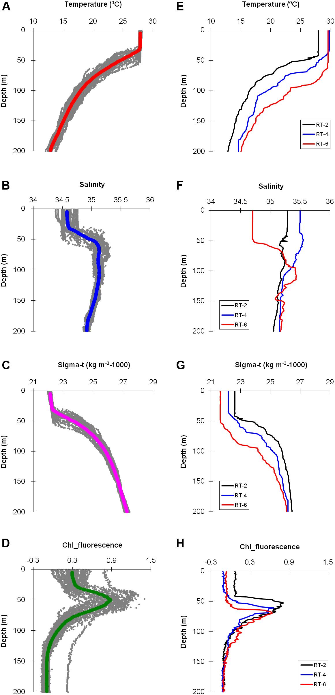
Figure 2. Vertical profiles of hydrographic parameters at TS (A–D) and RT (E–H) stations measured by CTD profiling. The solid line in time series profiles indicates mean value, whereas the dotted profiles denote all the casts performed. Legends for RT stations are given in respective figures.

The return track (RT) stations witnessed higher SST compared to TS stations, which varied from 29.0–29.9⁰C. Likewise, the vertical variation of temperature was also high, ranging between 12.8 and 29.8 (21.27 ± 5.99 ⁰C). Temperature profile of RT-2 was different (cooler) compared to the other two stations (Figure 2E), whereas RT-6 depicted deeper MLD, probably due to the intrusion of low-saline warm water from north EIO region as evidenced by lower salinity values at RT-6 (Figure 2F). However, relatively higher salinity was observed at RT stations with vertical profile varying from 34.69–35.55 (35.19 ± 0.20). Decease in water density, deepening of MLD, SCM (Figure 2H), and Z_eu (Table 1) was observed toward the EIO region. Similar to TS station, the MLD was always shallower than the depth of SCM and Z_eu signifying favorable light environment for phytoplankton production within the MLD (Westwood et al., 2011). There was a significant positive relationship between SCM and MLD for entire study region (r = 0.69, n = 43, p < 0.001).

Phytoplankton Biomass, Nutrients, and PAR

Vertical profiles of different parameters concurrently collected along with the PP measurements (on 9, 11, 13, and 15 June) are only discussed here. At TS station, surface Chl-a (Chl₀) showed minimal variation ranging from 0.17 to 0.26 mg m^–3 (Table 1); whereas vertical variation was more pronounced (Figure 3A) with concentrations ranging from not detectable quantity (ND) to 0.54 (0.23 ± 0.15 mg m^–3). Disparity in SCM depths was noticed for different days, which varied between 40−60 m as corroborating the Chl-a fluorescence data obtained from CTD. The column (up to 120 m)-integrated Chl-a (Chl_int) was moderately low and varied between 22.7 and 37.9 mg m^–2 (Table 1). Concentrations of macronutrients, i.e., nitrate (NO₃), phosphate (PO₄), and silicic acid or silicate (SiO₄) were nearly stable and low in the mixed layer (ML), showing gradual increase with depth (Figures 3B–D). NO₃ was almost ND in the ML, indicating its limitation. However, all nutrient concentrations below the ML were higher than surface waters suggesting that NO₃ and/or Si-limitation for diatoms/silicoflagellates were lesser at deeper depth. In general, the nutrient ratios were lower than the classical Redfield ratio (N:P:Si = 16:1:16) throughout the water column, where the mean N:P, N:Si, and Si:P ratios were 3.74 (±3.86), 0.41 (±0.41), and 6.93 (±3.49), respectively, indicating N-limited conditions (N:P <10 and N:Si <1; Levasseur and Therriault, 1987; Paul et al., 2008), and higher SiO₄ concentrations relative to NO₃ at TS station. Furthermore, data suggests that SiO₄ (<5 μM) was highly limited for diatoms and/or silicoflagellates growth (Westwood et al., 2011) and for other phytoplankton groups, whereas NO₃ was limiting, especially in the ML. Nevertheless, Si:P ratio was <3 throughout the water column showing Si-enrichment (Harrison et al., 1977) especially below the MLD. Water column PAR varied from 0–1899 (11.45 ± 60.46 μE m^–2 s^–1). Daily integrated surface PAR (D_PAR) was high (∼42 E m^–2 d^–1) during the sampling period; however, low D_PAR (∼19.4 E m^–2 d^–1) observed on 11 June (Table 1) was ascribed to the prevailing overcast sky condition.

FIGURE 3

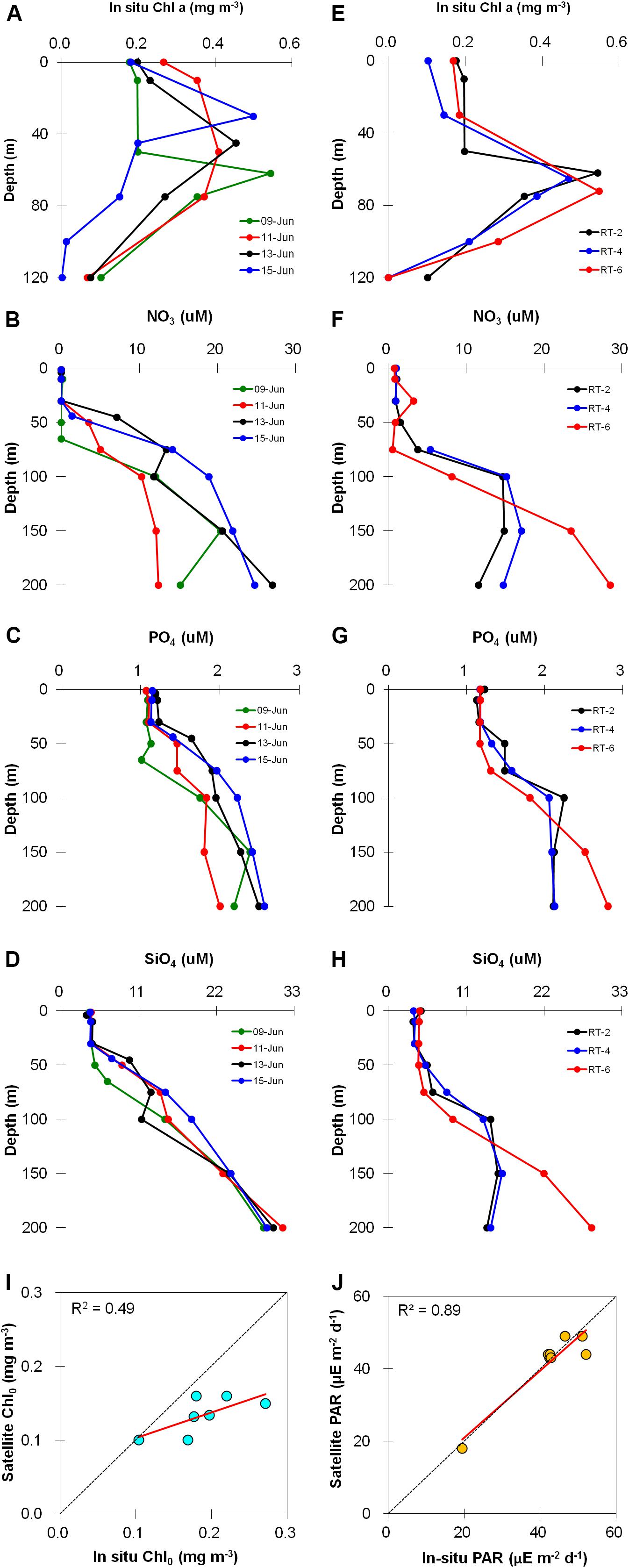
Figure 3. Depth profiles of phytoplankton biomass (only for the locations where primary productivity was measured), and nutrients for TS (A–D) and RT (E–H) stations. Scatter plots of (I) chlorophyll a and (J) photosynthetically active radiation measured by in situ and satellite remote sensing methods. Legends for TS and RT stations are given in respective figures. The dotted diagonal line indicates 1:1 relationship.

Similar to TS station, Chl₀ variation was insignificant at RT stations (Table 1) and showed distinct vertical variation ranging from ND to 0.54 (0.25 ± 0.18 mg m^–3). Compared to TS station, SCM was located at deeper depths (Figure 3E) coinciding with CTD-based fluorescence measurements. The Chl_int was slightly higher and laid between 28.3 and 39.4 mg m^–2 (Table 1). Correlation between Chl₀ and Chl_int was weak and insignificant (r = 0.4, p > 0.05) for the entire study area (figure now shown) emphasizing that sub-surface Chl-a has more contribution toward magnitude of Chl_int. Nutrients concentrations (Figure 3F–H) and ratios were virtually identical to TS station indicating depletion of NO₃ and SiO₄ in the ML, and enrichment of N and Si below the MLD. Intensity of D_PAR varied between 46.5 and 52.0 E m^–2 d^–1 (Table 1) and was higher for the stations depending on its proximity to the equator. The vertical light attenuation coefficient (k_d) varied from 0.051–0.070 (avg. 0.061 m^–1) and 0.044–0.068 (avg. 0.058 m^–1) at TS and RT stations, respectively (Table 1). No correlation between k_d and Chl_int was observed. Light climate, i.e., the mean PAR levels available to the phytoplankton in the ML (E_ML), varied from 6.7–18.4 and 16.0–19.8 E m^–2 d^–1 at TS and RT stations, respectively (Table 1). Variation in D_PAR and E_ML between different sampling stations were insignificant (p > 0.05), and E_ML corresponded to 36–45% of the D_PAR in the study area.

Comparison of Chl₀ obtained from satellite and in situ measurements (Figure 3I) resulted in underestimation by satellite and showed a moderate (r = 0.49, n = 7), insignificant (p ≤ 0.07) correlation. Conversely, the observed D_PAR values were significantly correlated (r = 0.94, n = 7, p < 0.001) with its satellite-based counterparts (Figure 3J).

Phytoplankton Pigments Signatures

Fluorometrically measured size-fractionation of surface Chl-a data at TS station (Figure 4A) revealed dominant contribution from smaller (flagellates, nano- and pico-sized) phytoplankton (0.2−10 μm) representing 55–93% (avg. 72%) of the total Chl-a, which ranged from 0.18 to 0.26 mg m^–3. Since Chl-a size-fraction data was unavailable, the % contribution of smaller and larger phytoplankton to the total Chl-a could not be quantified for RT stations. Through, HPLC-based analyses we could segregate different photosynthetically active marker pigments for diatoms (fucoxanthin) and dinoflagellates (peridinin), both signifying micro-plankton (large cells); prymnesiophytes (19’HF) and chrysophytes (19’BF) representing nano-plankton (small cells); and synechococcus (zeaxanthin) and prochlorococcus (divinyl chlorophyll-a and divinyl chlorophyll-b), both characterizing pico-plankton (small cells). Size-fractioned analysis of phytoplankton pigments showed an average of 22%, 53%, 25% contributions by micro-plankton (f_micro), nano-plankton (f_nano), and pico-plankton (f_pico), respectively, indicating dominance of nano-sized plankton in the TS stations almost throughout the study period (Figure 4B). Though the micro-plankton % remained stable during the TS measurements, a sharp decline in nano-plankton was observed on the 8^th day (16 June) that coincided with increase in pico-plankton community in the surface layer. Size-fractionated contributions and vertical distribution pattern of plankton in the water column were similar to surface layer (see Supplementary Material).

FIGURE 4

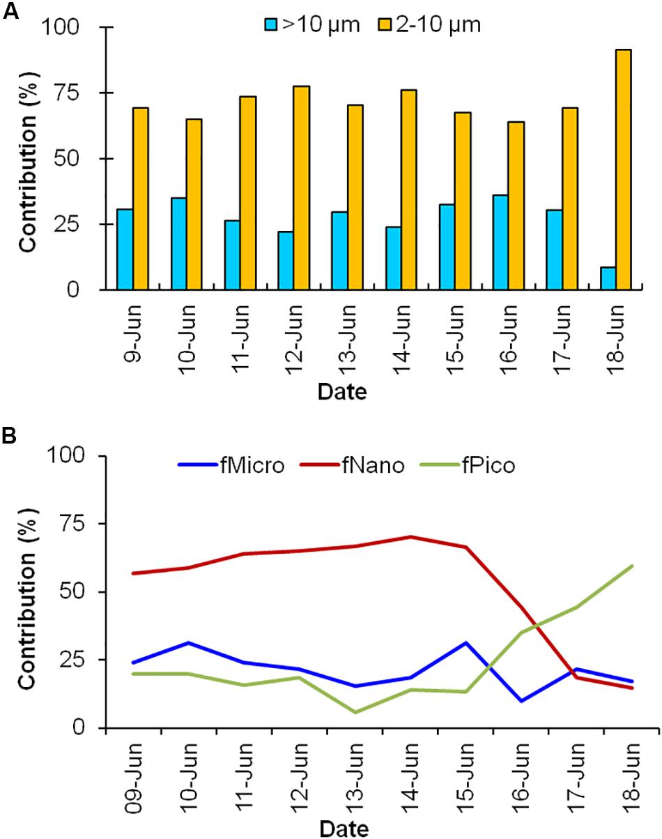
Figure 4. Size-fractionated contribution (%) of phytoplankton community structure measured by (A) fluorometric and (B) HPLC-based pigment analysis in the surface layer of the TS station.

Primary Production Variability

Measured PP in near-surface waters were low (∼2 mgC m^–3 d^–1) and at discrete depths ranged from 5.83 mgC m^–3 d^–1 in subsurface waters, down to 0.56 mgC m^–3 d^–1 at the Z_eu (Figure 5A). Column integrated production (IPP) varied from 176–268 (241 ± 43 mgC m^–2 d^–1) and was relatively stable during the observation period, except with low value for TS-14 (Table 1), which was ascribed to the drastic dropdown in the available D_PAR on that particular day due to overcast sky. Higher PP rates in the subsurface layers were directly related to higher Chl-a concentrations (Figure 3A). Vertical profiles of PP followed the distribution pattern of Chl-a within and below the ML and usually showed maximum values corresponding to SCM depths (∼10% of surface PAR). The assimilation number or Chl a-specific PP (P^B) varied from 1.6–16.7 (9.7 ± 4.1 mgC [mgChl-a]^–1 d^–1), and was mostly higher within the ML (Figure 5B) showing minimal/no surface photoinhibition (Figure 5C), which is indicative of probable dominance of smaller cells (Bricaud et al., 1995; Westwood et al., 2011) in the surface layer. Comparatively, higher P^B within the ML indicated that cells within this layer were healthy during the sampling time. Low P^B below the SCM depth could be due to light limitation.

FIGURE 5

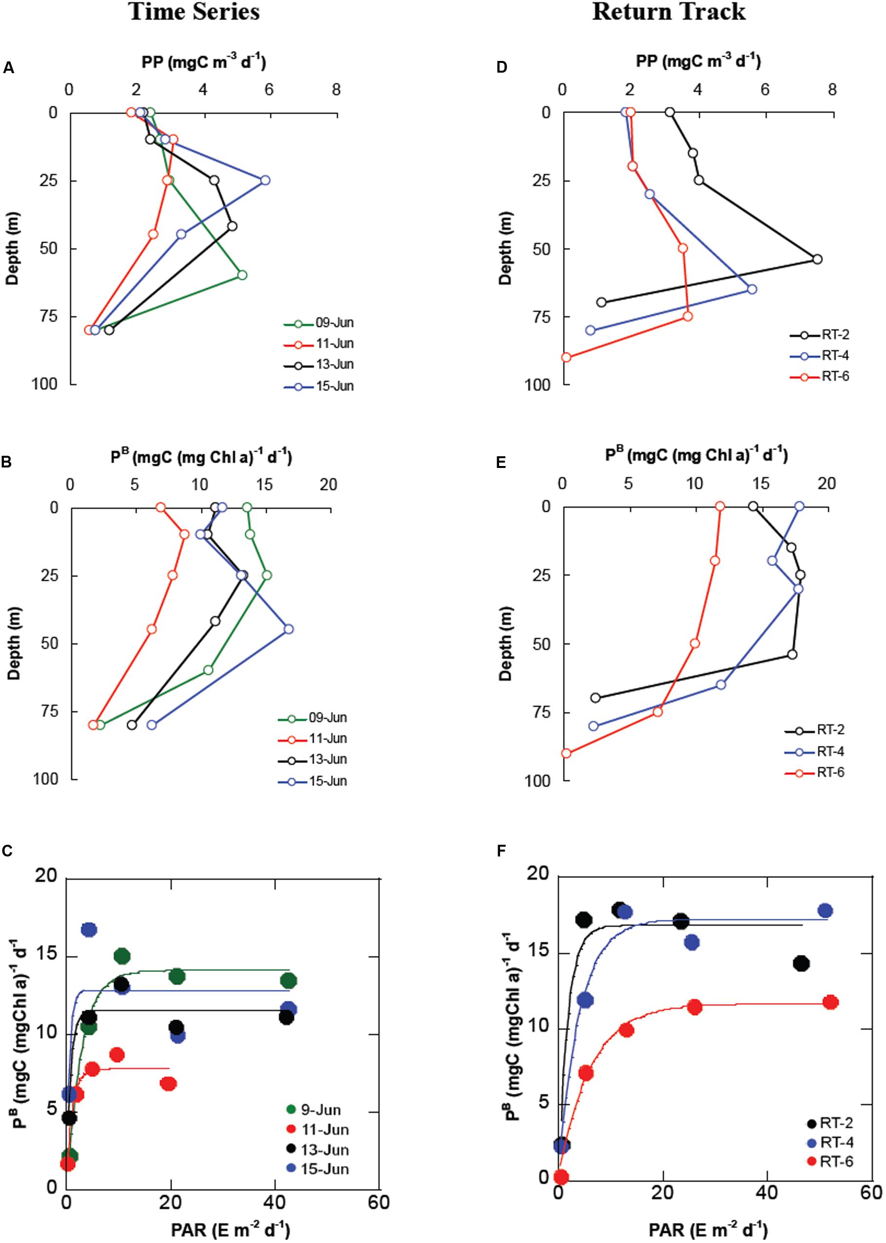
Figure 5. Vertical profiles of primary productivity, chlorophyll a-normalized primary productivity, and daily PAR-P^B relationship in the water column for TS (A–C) and RT (D–F) stations.

Analogous to TS station, the PP at surface layer of the RT stations (Figure 5D) were low and at discrete depths it ranged from 0.09–7.52 (2.9 ± 1.9 mgC m^–3 d^–1). Average IPP was relatively higher (274 mgC m^–2 d^–1) than the TS stations. Like TS station, vertical profiles of PP rates resembled the distribution pattern of Chl-a, where the depths of maximum PP were observed below the MLD nearly coinciding with the SCM depths. The P^B (Figure 5E) varied from 0.25–17.8 mgC (mgChl-a^–1 d^–1) with higher average (11.4 ± 6.7) compared to TS stations. PAR-P^B relationship indicated minimal/no surface photoinhibition (Figure 5F). Unlike TS station, surface P^B maximum was observed at RT-4 and RT-6, whereas subsurface P^B maximum, within the ML, was observed at RT-2. No surface photoinhibition and higher P^B in the surface and ML indicates probable preponderance of smaller phytoplankton communities (Bricaud et al., 1995; Westwood et al., 2011). Chl-a at discrete depths yielded in a significant positive and negative linear relationship (see Supplementary Material) with PP (r² = 0.19, n = 36, p < 0.05) and P^B (r² = 0.18, n = 36, p < 0.05), respectively. Inverse relationship between P^B and Chl-a implied decreasing photosynthetic efficiency with increasing biomass in the study area.

Comparison of measured and model (VGPM)-based IPP showed insignificant, weak correlation (r² = 0.24, n = 6) for the entire study area (Figure 6), yet, a close look at the data suggests that the measured and model-based IPP were strongly correlated for the RT stations (3 data points close to 1:1 line), conversely the calculated IPP underestimated (2.6 to 3 times) the measured IPP in TS stations. This underestimation could solely be linked to the difference in satellite-derived and measured Chl₀ concentrations that were fairly matching for the RT stations, whereas reasonably incongruous for the TS stations. Nevertheless, the results showed that a global model VGPM with its original parameterization can be used for precise estimation of IPP in this region. Since IPP on 14 June 2014 could not be calculated, that data has been removed from comparison.

FIGURE 6

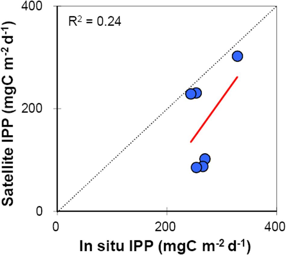
Figure 6. Linear relationship between in situ and satellite-derived primary productivity measurements (r² = 0.24, n = 6, p > 0.05). The dotted line indicates 1:1 relationship. Data points close to (away from) the 1:1 line belong to RT (TS) stations, respectively.

To further understand the observed variability in IPP, relationship measured between IPP, and surface variables (those are embedded in the VGPM model) were investigated. Among the sea surface variables, D_PAR showed a moderately linear (r² = 0.45, n = 7) but insignificant (p > 0.05) relationship with measured IPP (Figure 7A). Furthermore, there was no clear relationship between measured IPP and SST (Figure 7B) and Chl₀ (Figure 7C). The only significant correlation (r² = 0.73, n = 7, p < 0.05) observed was between IPP and P^B_opt (Figure 7D). The P^B_opt, which is a key parameter in satellite-based modeling of IPP ranged from 8.72 (TS-14) to 17.81 (RT-2) mgC (mgChl-a)^–1 d^–1 accounting for 73 % of variance in the measured IPP.

FIGURE 7

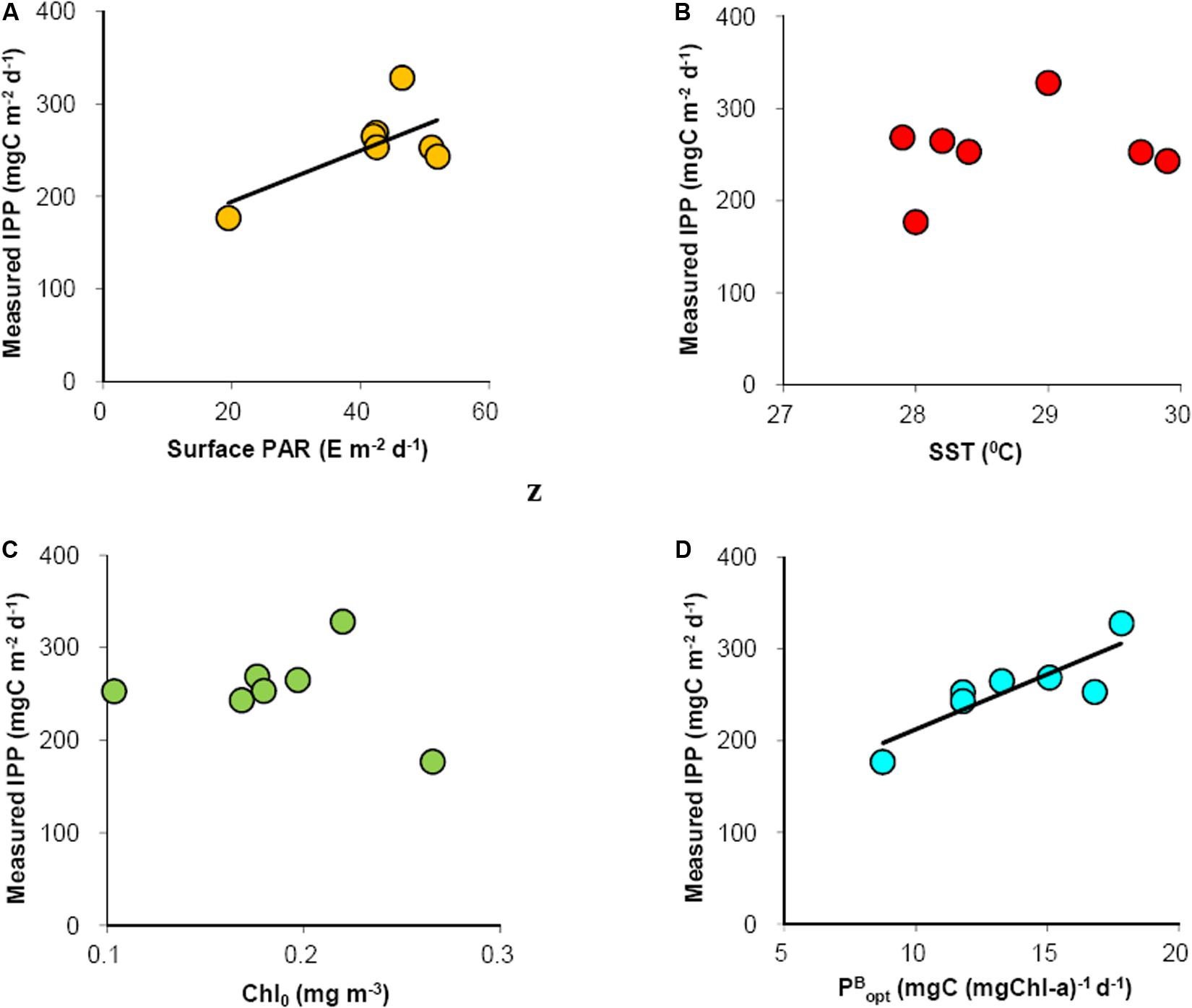
Figure 7. Linear relationships between measured IPP and (A) surface PAR (r² = 0.41, p < 0.05), (B) SST, (C) Chl₀, and (D) P^B_opt (r² = 0.73, p < 0.05). Trend line for figure b and c are not shown due to absence of any clear trend.

Discussion

Factors Governing Phytoplankton Community Composition and Production: Implication on Export Flux and Transfer Efficiency

Phytoplankton are enormously dissimilar in terms of their taxonomy, morphology, and size spanning over 10 orders of magnitude in cell volume (Margalef, 1978; Cullen et al., 2002). Ambient physicochemical factors (i.e., temperature, nutrient, and light availability) are often decisive for regulating growth of a particular phytoplankton species and its relative contributions to community structure (Reynolds and Reynolds, 1985). Thus, phytoplankton community structure can be regarded as an integral response of ambient environmental factors (Claustre et al., 2005). Phytoplankton forms the base of the oceanic food-web and performs a pivotal role in biogeochemical processes (especially influencing the efficiency of the carbon [C] export to the deep ocean through “biological pump”), which is an important component of global ocean C-sequestration and modulation of atmospheric CO₂.

During this study, shallow thermocline was observed with minimal thermohaline variations in the upper 35–40 m (Figure 2). Occurrence of low saline and warm water mass formed a stratified surface layer restricting MLD to 35–40 m. The stratification, with its determinant influence on upward nutrients fluxes, restricted the vertical mixing and prevented supply of nutrients from deeper layers resulting in macronutrients depletion in the MLD (Figure 3). The vertical position of the maximum Chl-a fluorescence (SCM) was located near or below the nitracline (vertical gradient of nitrate availability) in both TS and RT stations (Figures 2, 3) possibly reflecting phytoplankton adaptive strategies. Extremely high Z_eu-MLD values (>35 m) indicated that light availability within the ML was highly favorable for growth of phytoplankton (Westwood et al., 2011) during the observation period. The N:P:Si ratios were lower than Redfield values indicating NO₃ and SiO₄-limited conditions (N:P < 10 and N:Si < 1; Levasseur and Therriault, 1987; Paul et al., 2008) for diatoms and/or silicoflagellates growth (Westwood et al., 2011) in the ML throughout the sampling region. Nevertheless, Si:P ratio was <3 throughout the water column showing Si-enrichment (Harrison et al., 1977) especially below the MLD. The nutrient-limited conditions were well reflected in the Chl-a size-fractionation and phytoplankton pigment signatures data, which have clearly shown that the study area was dominated (55–93%) by smaller phytoplankton (0.2–10 μm) and the contribution of nano-plankton was highest (53%) followed by pico (25%)- and micro-plankton (22%). The most abundant pigments at TS location were 19′HF, which is used as markers for prymnesiophytes (Phaeocystis sp.) (Jeffrey et al., 1997). The next most dominant pigment was alloxanthin (indicating cryptophytes). Fucoxanthin (indicating diatoms) percentage was comparatively high in the first 8 days but was less/absent during the 9^th and 10^th days, which witnessed rise in TChl-b and 19′BF concentrations indicative of dominance of pico-plankton (Seeyave et al., 2007). This kind of shift/succession in phytoplankton community structure could be ascribed to the vertical stratification-induced nutrient-stress prevailing in this region, as reported in other tropical and temperate marine ecosystems (Margalef, 1978; Cullen et al., 2002). In other words, the vertical stratification can also determine the intensity and phytoplankton communities of the SCM. Furthermore, the difference between Z_eu and nitracline depth can therefore be a useful indicator of phytoplankton communities inhabiting at the SCM depth (Ardyna et al., 2011).

In general, small phytoplankton predominates in stable oligotrophic (open ocean) environments, while larger cells dominate in variable eutrophic (coastal and upwelling) environments (Chisholm, 1992), and their cell size has been shown to regulate the export efficiency of organic matter in the water column (Dunne et al., 2005; Guidi et al., 2009; Mouw et al., 2016). Dominance of smaller plankton in the phytoplankton community of the study area implies that the SWTIO region would experience lower carbon transfer efficiency and high export flux efficiency since the portion exported by small cells is generally less refractory, thus, sinks slower, resulting in lower transfer efficiency. Conversely, larger cells are more vulnerable of being associated with ballasting materials and thus leads to greater transfer efficiency (Klaas and Archer, 2002; Armstrong et al., 2009; Mouw et al., 2016). Previous study shows that the magnitude and export efficacy of carbon flux are dependent on the size of the phytoplankton cells prevailing in the ecosystem (Mouw et al., 2016). As a whole, the carbon export variability in a system is not only regulated by the phytoplankton cell size but also by zooplankton grazing and other components (particle aggregation and feces production) of the food-web (Siegel et al., 2014).

Increase in Chl-a concentration is usually associated with an increase in intracellular pigment concentration or cell volume rather than in cell number leading to decrease in phytoplankton light absorption efficiency (due to intracellular overlapping of the chloroplasts) is popularly known as “package effect” (Bricaud et al., 1995). Thus, the observed decrease in Chl-a-specific PP (P^B) in the surface layer is hypothesized to be caused by the onset of “package effect” (Bricaud et al., 1995), which is obvious in large (>10 μm) or micro-phytoplankton (diatoms) compared to small size (nano or pico) plankton. We observed minimal or no decrease in the PAR-P^B relationship in the surface layer at TS (Figure 5C) and RT (Figure 5F), which is indicative of absence of photoinhibition in the study area. Tripathy et al. (2010, 2014) have reported package-effect induced decrease in PP in eutrophic coastal waters of temperate and polar regions, and attributed this to dominance of large-sized phytoplankton. However, low nutrients availability in the ML have shown that the conditions were supportive for the growth of smaller phytoplankton (flagellates, nano- and pico-sized) that can efficiently utilize the low concentrations of nutrients due to their high surface to volume ratio. This canonical hypothesis was supported by the HPLC-based DP analysis corroborating the dominance of nano-sized plankton in the surface as well as in the water column.

Ocean warming-induced decline in the spatial coverage and temporal occurrence of micro-plankton has been observed due to significantly reduced nutrients in the ML in the major biogeochemical provinces of the world ocean (Rousseaux and Gregg, 2015). Recent study pointed out an astounding decrease (up to 20%) in phytoplankton in western tropical Indian Ocean region over the past 60 years (Roxy et al., 2016) caused by warming-induced enhanced ocean stratification that restrains mixing of nutrients from subsurface layers. Gao et al. (2012) have shown that increased CO₂ and light exposure have adverse impacts on the growth of marine phytoplankton causing extensive reduction in oceanic PP and a shift in community structure away from diatoms that are mainly accountable for sustaining higher trophic levels and export of carbon in the ocean. If spatiotemporal dominance of small cells continues, this may result in less but efficient export of materials leading to reduced POC transfer to the deep ocean. This has possible cascading implications for both atmospheric drawdown of CO₂ and C-sequestration in the deep ocean. Yet, there are some small diatoms (such as Minidiscus) that can reach the ocean bottom at high sinking rates, hence challenging the classical binary vision of pico- and nanoplanktonic cells supporting the microbial loop, while micro-plankton sustain secondary trophic levels and carbon export (Leblanc et al., 2018) in the ocean.

Comparison of Measured and Modeled Primary Production: Implications of P^B_opt on IPP Variability

The major inaccuracy in VGPM-based estimates of IPP are associated with estimations of P^B_opt, which is a key variable in PP modeling, yet is inadequately explained, and its predictability requires further refinement (Behrenfeld and Falkowski, 1997b; Kameda and Ishizaka, 2005; Siswanto et al., 2006; Hyde et al., 2008; Tripathy et al., 2012). Satellite-based estimates of P^B_opt can be derived by establishing predictive relationships between P^B_opt and one or more environmental variables (e.g., temperature, light, Chl-a), which can be measured by satellites (Behrenfeld et al., 2002). The following section elucidates the importance of P^B_opt in modeling primary production in the studied region.

Our results showed that VGPM, a global model with its original parameterization, could be used for precise estimation of IPP in the RT stations (3 data points close to 1:1 line); however, the modeled IPP underestimated (2.6 to 3 times) measured IPP at TS stations (Figure 6). This underestimation could be attributed to the difference in satellite-derived and measured Chl₀ concentrations that were fairly matching for the RT stations, whereas reasonably incongruous for the TS stations. It has been shown that, next to P^B_opt, the Chl₀ has significant contribution toward the errors associated with VGPM-based IPP estimates (Behrenfeld and Falkowski, 1997b). Analysis of measured IPP vs. in situ variables (those are embedded in the VGPM model) indicated that only in situ P^B_opt was significantly correlated (r² = 0.73, n = 7, p < 0.05) with IPP (Figure 7D) accounting for 73% of variance in measured IPP. Thus, it is presumed that the discrepancies in measured and modeled IPP at TS stations could be due to errors in estimating P^B_opt.

In this study, no distinct relationships were observed between the in situ P^B_opt and SST, PAR, and/or Chl-a; thus, a P^B_opt model using the above oceanographic variables was not feasible in SWTIO region. Also, due to small in situ dataset (n = 7), fitting any kind of relationship function between P^B_opt and other oceanographic variables was not realistic. Previously attempts to construct SST-dependent P^B_opt models (Behrenfeld and Falkowski, 1997b; Gong and Liu, 2003; Kameda and Ishizaka, 2005; Siswanto et al., 2006) have shown varying shapes for the P^B_opt function. Our results depicted that the derivation of P^B_opt by adopting the above model formulations was not effective (Figure 8) in this region. The observed P^B_opt and SST relationship of this study resembles the observations at Cariaco station, southeastern Caribbean Sea (Muller-Karger et al., 2004) and in the East China Sea (Siswanto et al., 2006), where consistent increase in P^B_opt was noticed even at SST as high as 29^oC. Our data show that the P^B_opt increased with increasing SST until 29°C and then decreased, which is not in line with the global seventh-order polynomial P^B_opt model (Behrenfeld and Falkowski, 1997b), as well as SST and Chl₀ dependent P^B_opt model (Kameda and Ishizaka, 2005). Both models showed decline in P^B_opt with increasing SST (Figure 8), and opined that persistent nutrient limitation in the strongly stratified high SST regions lead to decline in P^B_opt at higher SST. Such discrepancy could possibly be accountable for the ineffectiveness of VGPM to capture measured IPP variance at TS station.

FIGURE 8

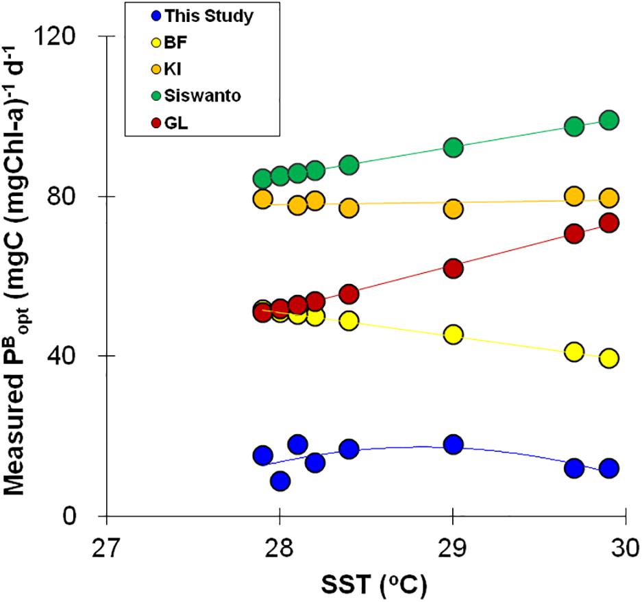
Figure 8. Relationships between measured P^B_opt and SST. Circles, stars, diamonds, triangles, and squares indicate P^B_opt variations based on datasets of this study, models of Behrenfeld and Falkowski (1997a), Gong and Liu (2003); Kameda and Ishizaka (2005), Siswanto et al. (2006), respectively.

Temperature exclusively was unable to explain the variation in P^B_opt, because P^B_opt variation was plausibly influenced by the cumulative effects of nutrient concentrations, total biomass, light history, day-length, phytoplankton composition, and size that are independent of temperature (Cote and Platt, 1983; Behrenfeld and Falkowski, 1997b). Thus, a single-factor, statistical P^B_opt model may not capture the physiological adjustments by phytoplankton with respect to the surrounding growth conditions (Behrenfeld and Falkowski, 1997b), and warrant development of a mechanistic model (e.g., Kameda and Ishizaka, 2005). Constant P^B_opt values have been used to estimate IPP elsewhere (Dierssen et al., 2000; Hyde et al., 2008) when reliable derivation of P^B_opt using environmental variables failed. Developing a P^B_opt model was out of scope of this study and hence not attempted because of the small dataset.

The other likely justification for the poor performance of VGPM at TS station is that the optical property of this study region may not be resembling the domain (i.e., Chl-a is the major determinant of the water optical properties) in which VGPM was formulated. Absence of correlation between k_d and Chl_int implied that the study area was optically complex, where constituents other than Chl-a (such as suspended sediments, chromophoric dissolved organic matter) could be playing a main role in determining light attenuation in the water column. Alas, due to lack of data on other optically active constituents we could not verify this. The observed k_d values (Table 1) were similar for both TS and RT stations indicating identical optical properties. Thus, observed discrepancies between measured and modeled IPP at TS and RT stations could only be attributed to the differences in satellite-derived and in situ Chl₀.

Physical Forcings Associated With the Observed High Productivity at RT-2

Throughout the year, the SCTR experiences upwelling due to the upward Ekman suction (Murtugudde et al., 1996; Spencer et al., 2005). Previously it was shown that the interannual variability of the thermohaline stratification in the SCTR region is primarily caused by the equatorial zonal wind anomalies caused by the Indian Ocean Dipole (IOD). The IOD induces a strong Ekman suction south of the equator including the eastern and central Indian Ocean, which subsequently move westward under the influence of planetary wave dynamics (Masumoto and Meyers, 1998), thereby modulating the biogeochemistry of the SCTR region.

During the study period highest Chl_int (39.4 mg m^–2) and IPP (328.1 mgC m^–2 d^–1) was observed at RT-2. To investigate the possible role of physical forcings on the observed high phytoplankton biomass and productivity at RT-2, we analyzed sea surface height anomaly (SSHA) coupled with geostrophic currents during the sampling period. Interestingly, the SSHA plots highlighted that the observed high Chl-a region was well inside negative SSHA regions (Figure 9A, top right panel) as observed elsewhere (Sabu et al., 2014). Previous study (George et al., 2013) correlated the negative (in SCTR region) and positive (near the equator and south of the SCTR region) SSHA to shallower and deeper thermocline, respectively. The observed negative SSHA could be linked to the Ekman suction velocity calculated for the study area, which showed a surge on 6^th June signaling possible upwelling during this period (Figure 9B). The elevated Ekman suction velocity could have upwelled nutrient-rich waters thereby enhancing phytoplankton growth. It is well documented that strong Ekman suction deepens the surface ML considerably and Chl peaks when SSHA decreases in SCTR region (Resplandy et al., 2009). MODIS-Aqua-derived Chl-a images (Figure 9C) confirmed presence of high Chl patch near to RT-2 well before the observation date (28^th May to 9^th June), which persisted till 26^th June. Since the intensity and spatial extension of the Chl increased in the last week of June, the high Chl observed in our study had originated from this high Chl patch. Furthermore, the high surface Chl might have resulted not only from the entrainment of subsurface Chl but also from the influx of nutrients and phytoplankton production in the ML (Resplandy et al., 2009).

FIGURE 9

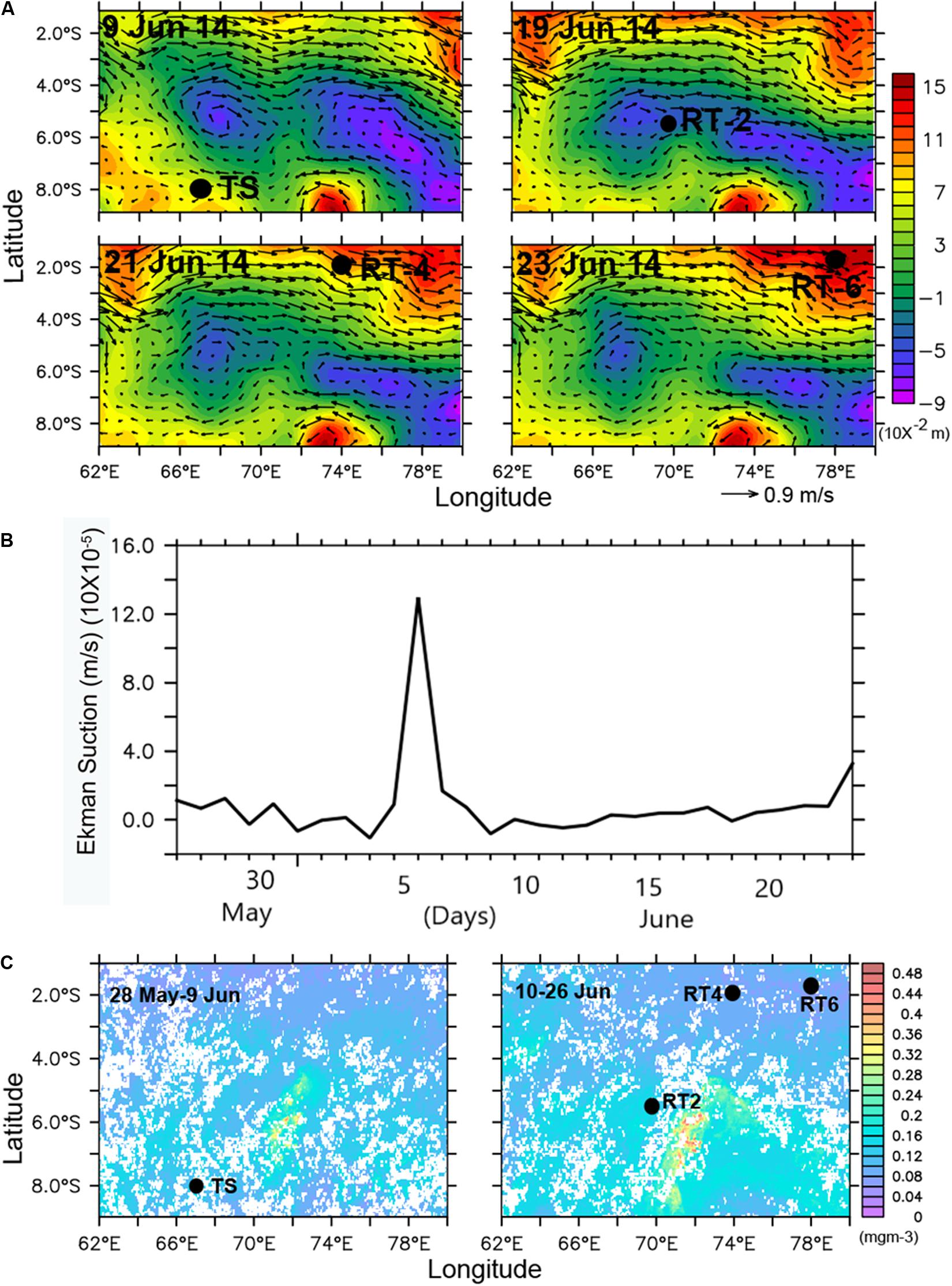
Figure 9. (A) spatial distribution of sea surface height anomaly (SSHA) overlaid on geostrophic wind vectors (top right panel corresponds to RT-2, black dots denote the station locations), (B) average Ekman suction velocity at RT-2 region (6S:5S and 69E:70E) during May–June 2014 showing peak on 6 June, and (C) MODIS-Aqua derived weekly average level-3 chlorophyll images (black dots symbolizes station locations) indicating high chlorophyll-a patch at RT-2.

Moreover, analysis of SST images indicated that RT-4 and RT-6 were in higher SST region than TS and RT-2 (Figure 10A), and SST in the RT-2 was colder on 9^th June than on 19^th June, indicating upwelling signatures. So the cooler water on 9^th June was triggered by the high Ekman suction velocity just 3 days before, corroborating that the SCTR region is significantly influenced by Ekman-suction-induced upwelling, driven by the northward decrease of the southeast trade wind (Vialard et al., 2008). Analysis of surface wind data for this period indicated that the high Ekman suction/low SSHA in the RT-2 region was due to the occurrence/passage of a high wind event on 6^th June (Figure 10B) that’s enhanced Ekman suction and favored entrainment of nutrients to the surface layer, in consequence enhancing phytoplankton growth and photosynthetic activity. Thus, the high Chl_int and IPP at RT-2 on 19^th June was due to occurrence of an upwelling event before our observation. Previous report (Spencer et al., 2005) shows that the annual mean upwelling in the SWTIO is associated with wind driven Ekman suction. Our result is consistent with the findings of George et al. (2013), who have revealed Ekman suction-induced variability in MLD and increase in surface Chl by entrainment of nutrients from deeper layers in the SCTR region.

FIGURE 10

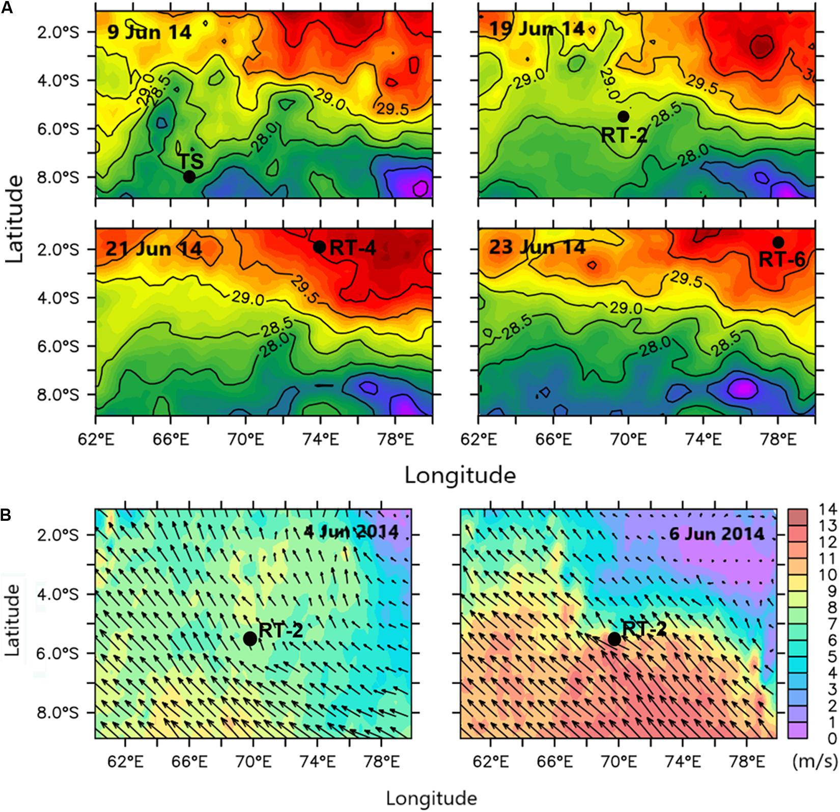
Figure 10. (A) Sea surface temperature (SST) variability during the observation period, and (B) surface wind pattern during 4 and 6 June. Black dots signify station locations.

Unlike RT-4 and RT-6, we observed subsurface P^B_opt for RT-2 station (Figure 5F), which indicates that the reduced phytoplankton photosynthetic efficiency in the surface layer was probably due to the light-shock the plankton experienced when they were transported from deeper to shallower regions. Earlier study documents that vertical displacements of phytoplankton, due to mixing, force phytoplankton to experience fast alterations in underwater light intensity (Shibata et al., 2010), which exposes the phytoplankton cells to higher PAR, causing damages to the photosynthetic apparatus and photoinhibitory decrease in the photosynthetic efficiency (Falkowski et al., 1994). The PAR-P^B relationship showed mild photoinhibition (Figure 5F) at RT-2, which could be attributed to the less pigment packaging due to dominance of nano-plankton during the sampling period. Similar observations (Tripathy et al., 2014) were also reported in the offshore waters of Southern Ocean where nutrient-limitation induced predominance of smaller plankton existed.

Summary and Conclusion

To our knowledge, this is the first in situ measurement-based study describing the factors modulating phytoplankton productivity and composition in the SCTR region. Our study not only confirmed some of the earlier reports about variability in phytoplankton biomass but also provides first-hand information about the in situ variability in phytoplankton pigment signatures and carbon-uptake efficiency. Some of the conclusions drawn from this study are summarized below.

The SCTR region is usually oligotrophic in nature in the month of June. Strong thermohaline stratification resulted in shallow (35–40 m) mixed layer (ML). Subsurface Chl-a maximum (SCM) was a prominent feature and observed to oscillate 40–60 m with majority of peaks at 50 m, and existed just beneath the ML depth. Light availability during the sampling period was highly conducive for algal growth, whereas nutrient ratios indicated N- and Si-limitation suggesting unfavorable conditions for diatoms and/or silicoflagellates growth within the ML. Moreover, dominance of nano-sized plankton (53%) followed by pico-plankton (25%) and micro-plankton (22%) could be confirmed by HPLC-based pigments analysis. Drastic dropdown in daily incident light due to overcast sky can severely influence the IPP even though other supporting parameters remain unchanged. In the vertical profiles maximum PP usually coexisted to SCM depths. The Chl-a-specific PP (P^B) was higher within the ML and showed no surface photoinhibition, due to the dominance of smaller phytoplankton, which are less prone to pigment packaging effect. Comparatively, higher P^B within the ML is indicative of phytoplankton healthiness during the sampling time, whereas low P^B below the SCM was due to light limitation. The highest column integrated phytoplankton biomass (Chl_int) and productivity (IPP) observed at RT-2 could be clearly linked to low sea surface height anomaly (SSHA); cyclonic disturbances and associated positive Ekman suction velocity occurred before our observation period. Conversely, high SSHA and strong stratification conditions prevailed at other stations (TS, RT-4, and RT-6) leading to comparatively low Chl_int and IPP. Though dominance of smaller phytoplankton were observed in the study area, future work focusing on grouping of phytoplankton into functional types will have more interest to the biogeochemical community because they are relevant indicators of ecosystem dynamics and functioning vis-à-vis climate change, and may provide vital information about potential impacts on the efficiency of oceanic carbon sequestration which controls global climate change.

Data Availability Statement

The datasets generated for this study are available on request to the corresponding author.

Author Contributions

ST collected the primary production data, conceived the study, and wrote the manuscript. PS helped in processing satellite-based observations. SP, RN, AS, VV, AK, and PR contributed in generation of other in situ data and analyses. All authors contributed toward interpreting results, discussion, and improvement of this manuscript.

Funding

Financial assistance from the Ministry of Earth Sciences, Government of India is highly acknowledged.

Conflict of Interest

The authors declare that the research was conducted in the absence of any commercial or financial relationships that could be construed as a potential conflict of interest.

Acknowledgments

The authors are thankful to the Director, NCPOR and Group Director, Ocean Sciences Group for their constant encouragement and support. Exemplary assistance from the Captain, officers, and all crew members onboard ORV-Sagar Nidhi is sincerely acknowledged. This is NCPOR contribution number J-13/2020-21.

Supplementary Material

The Supplementary Material for this article can be found online at: https://www.frontiersin.org/articles/10.3389/fmars.2020.00515/full#supplementary-material

MATERIAL S1 | Size-fractioned contributions (average) of phytoplankton pigments in the water column at the TS station.

MATERIAL S2 | Scatter plots showing linear relationships between Chl a and (A) PP, and (B) P^B for the entire study area.

References

Annamalai, H. R., Murtugudde, J., Potemra, S. P., Xie, P. L., and Wang, B. (2003). Coupled dynamics over the Indian Ocean: spring initiation of the zonal mode. Deep-Sea Res. II 50, 2305–2330. doi: 10.1016/s0967-0645(03)00058-4

CrossRef Full Text | Google Scholar

Ardyna, M., Gosselin, M., Michel, C., Poulin, M., and Tremblay, J. E. (2011). Environmental forcing of phytoplankton community structure and function in the Canadian High Arctic: contrasting oligotrophic and eutrophic regions. Mar. Ecol. Prog. Ser. 442, 37–57. doi: 10.3354/meps09378

CrossRef Full Text | Google Scholar

Armstrong, R. A., Peterson, M. L., Lee, C., and Wakeham, S. G. (2009). Settling velocity spectra and the ballast ratio hypothesis. Deep Sea Res. II 56, 1470–1478. doi: 10.1016/j.dsr2.2008.11.032

CrossRef Full Text | Google Scholar

Behrenfeld, M. J., and Falkowski, P. G. (1997a). A consumer’s guide to phytoplankton primary productivity models. Limnol. Oceanogr. 42, 1479–1491. doi: 10.4319/lo.1997.42.7.1479

CrossRef Full Text | Google Scholar

Behrenfeld, M. J., and Falkowski, P. G. (1997b). Photosynthetic rates derived from satellite based chlorophyll concentration. Limnol. Oceanogr. 42, 1–20. doi: 10.4319/lo.1997.42.1.0001

CrossRef Full Text | Google Scholar

Behrenfeld, M. J., Maranon, E., Siegel, D. A., and Hooker, S. B. (2002). Photoacclimation and nutrient-based model of light-saturated photosynthesis for quantifying oceanic primary production. Mar. Ecol. Prog. Ser. 228, 103–117. doi: 10.3354/meps228103

CrossRef Full Text | Google Scholar

Behrenfeld, M. J., O’Malley, R. T., Siegel, D. A., McClain, C. R., Sarmiento, J. L., Feldman, G. C., et al. (2006). Climate-driven trends in contemporary ocean productivity. Nature 444, 752–755. doi: 10.1038/nature05317

PubMed Abstract | CrossRef Full Text | Google Scholar

Boyd, P. W., Jickells, T., Law, C. S., Blain, S., Boyle, E. A., Buesseler, K. O., Coale, K. H., et al. (2007). Mesoscale iron enrichment experiments 1993-2005: synthesis and future directions. Science 315, 612–617. doi: 10.1126/science.1131669

PubMed Abstract | CrossRef Full Text | Google Scholar

Bricaud, A., Babin, M., Morel, A., and Claustre, H. (1995). Variability in the chlorophyll-specific absorption coefficients for natural phytoplankton: analysis and parameterization. J. Geophys. Res. 100, 13321–13332.

Google Scholar

Cheah, W., McMinn, A., Griffiths, F. B., Westwood, K. J., Wright, S. W., et al. (2013). Response of phytoplankton photophysiology to varying environmental conditions in the sub-antarctic and polar frontal zone. PLoS One 8:e72165. doi: 10.1371/journal.pone.0072165

PubMed Abstract | CrossRef Full Text | Google Scholar

Chisholm, S. (1992). “Phytoplankton size,” in Primary Productivity and Biogeochemical Cycles in the Sea, eds P. G. Falkowski, A. D. Woodhead, and K. Vivirito (Berlin: Springer), 213–237.

Google Scholar

Claustre, H., Babin, M., Merien, D., Ras, J., Prieur, L., Dallot, S., et al. (2005). Towards a taxon-specific parameterization of bio-optical models of primary production: a case study in the North Atlantic. J. Geophys. Res. 110:C07S12. doi: 10.1029/2004JC002634

CrossRef Full Text | Google Scholar

Cote, B., and Platt, T. (1983). Day-to-day variations in the spring-summer photosynthetic parameters of coastal marine phytoplankton. Limnol. Oceanogr. 28, 320–344. doi: 10.4319/lo.1983.28.2.0320

CrossRef Full Text | Google Scholar

Cullen, J., Franks, P., Karl, D., and Longhurst, A. (2002). “Physical influences on marine ecosystem dynamics,” in The Sea, eds A. R. Robinson, J. J. McCarthy, and B. J. Rothschild (New York, NY: John Wiley), 297–336.

Google Scholar

Dierssen, H. M., Vernet, M., and Smith, R. C. (2000). Optimizing models for remotely estimating primary production in Antarctic coastal waters. Antarct. Sci. 12, 20–32. doi: 10.1017/s0954102000000043

CrossRef Full Text | Google Scholar

Dilmahamod, A. F., Hermes, J. C., and Reason, C. J. C. (2016). Chlorophyll-a variability in the Seychelles-Chagos Thermocline Ridge: analysis of a coupled biophysical model. J. Marine Syst. 154, 220–232. doi: 10.1016/j.jmarsys.2015.10.011

CrossRef Full Text | Google Scholar

Dunne, J., Armstrong, R., Gnanadesikan, A., and Sarmiento, J. (2005). Empirical and mechanistic models for the particle export ratio. Global Biogeochem. Cycles 19:GB4026. doi: 10.1029/2004GB002390

CrossRef Full Text | Google Scholar

Falkowski, P. G., Greene, R., and Kolber, Z. (1994). “Light utilization and photoinhibition of photosynthesis in marine phytoplankton,” in Photoinhibition of Photosynthesis: From Molecular Mechanisms to the Field, eds N. R. Baker and J. Bowes (Oxford: Bios Scientific).

Google Scholar

Gao, K., Xu, J., Gao, G., Li, Y., Hutchins, D. A., Huang, B. A., et al. (2012). Rising CO2 and increased light exposure synergistically reduce marine primary productivity. Nat. Clim. Change 2, 519–523. doi: 10.1038/NCLIMATE1507

CrossRef Full Text | Google Scholar

George, J. V., Nuncio, M., Chacko, R., Anilkumar, N., Noronha, S. B., Patil, S. M., et al. (2013). Role of physical processes in chlorophyll distribution in the western tropical Indian Ocean. J. Marine Syst. 113- 114, 1–12. doi: 10.1016/j.jmarsys.2012.12.001

CrossRef Full Text | Google Scholar

Gong, G. C., and Liu, G. J. (2003). An empirical primary production model for the ECS. Cont. Shelf Res. 23, 213–224. doi: 10.1016/s0278-4343(02)00166-8

CrossRef Full Text | Google Scholar

Guidi, L., Stemmann, L., Jackson, G. A., Ibanez, F., Claustre, H., Legendre, L., et al. (2009). Effects of phytoplankton community on production, size, and export of large aggregates: a world-ocean analysis. Limnol. Oceanogr. 54, 1951–1963. doi: 10.4319/lo.2009.54.6.1951

CrossRef Full Text | Google Scholar

Harrison, P. J., Conway, H. L., Holmes, R. W., and Davis, C. O. (1977). Marine diatoms in chemostats under silicate or ammonium limitation. III. Cellular chemical composition and morphology of three diatoms. Mar. Biol. 43, 19–31. doi: 10.1007/bf00392568

CrossRef Full Text | Google Scholar

Hermes, J. C., and Reason, C. J. C. (2008). Annual cycle of the South Indian Ocean (Seychelles-Chagos) thermocline ridge in a regional ocean model. 113, C04035. doi: 10.1029/2007JC004363

CrossRef Full Text | Google Scholar

Hyde, K. J. W., O’Reilly, J. E., and Oviatt, C. A. (2008). Evaluation and application of satellite primary production models in Massachusetts Bay. Cont. Shelf Res. 28, 1340–1351. doi: 10.1016/j.csr.2008.03.017

CrossRef Full Text | Google Scholar

Jeffrey, S. W., Mantoura, R. F. C., and Wright, S. W. (1997). Phytoplankton Pigments in Oceanography: Guidelines to Modern Methods. Paris: UNESCO Publishing.

Google Scholar

Jung, E., and Kirtman, B. P. (2016). ENSO modulation of tropical Indian ocean subseasonal variability. Geophys. Res. Lett. 43, 12634–12642. doi: 10.1002/2016GL071899

CrossRef Full Text | Google Scholar

Kameda, T., and Ishizaka, J. (2005). Size-fractionated primary production estimated by a two-phytoplankton community model applicable to ocean color remote sensing. J. Oceanogr. 61, 663–672. doi: 10.1007/s10872-005-0074-7

CrossRef Full Text | Google Scholar

Kirk, J. T. O. (1994). Light and Photosynthesis in Aquatic Ecosystems. Cambridge: Cambridge University Press, 509.

Google Scholar

Klaas, C., and Archer, D. E. (2002). Association of sinking organic matter with various types of mineral ballast in the deep sea: implications for the rain ratio. Glob. Biogeochem. Cycles 116:1116. doi: 10.1029/2001GB001765

CrossRef Full Text | Google Scholar

Kurian, S., Roy, R., Repeta, D. J., Gauns, M., Shenoy, D. M., Suresh, T., et al. (2012). Seasonal occurrence of anoxygenic photosynthesis in Tillari and Selaulim reservoirs, western India. Biogeosciences 9, 2485–2495. doi: 10.5194/bg-9-2485-2012

CrossRef Full Text | Google Scholar

Leblanc, K., Quéguiner, B., Diaz, F., Cornet, V., Michel-Rodriguez, M., Durrieu de Madron, X., et al. (2018). Nanoplanktonic diatoms are globally overlooked but play a role in spring blooms and carbon export. Nat. Comm. 9:953. doi: 10.1038/s41467-018-03376

CrossRef Full Text | Google Scholar

Levasseur, M. E., and Therriault, J. C. (1987). Phytoplankton biomass and nutrient dynamics in a tidally induced upwelling: the role of NO3: SiO4 ratio. Mar. Ecol. Prog. Ser. 39, 87–97. doi: 10.3354/meps039087

CrossRef Full Text | Google Scholar

Lohrenz, S. E., Wiesenburg, D. A., Rein, C. R., Arnone, R. A., Taylor, C. T., Knauer, G. A., et al. (1992). A comparison of in situ and simulated in situ methods for estimating oceanic primary production. J. Plankton Res. 14, 201–221. doi: 10.1093/plankt/14.2.201

CrossRef Full Text | Google Scholar

Longhurst, A. R., and Harrison, W. G. (1989). The biological pump: profiles of plankton production and consumption in the upper ocean. Prog. Oceanog. 22, 47–123. doi: 10.1016/0079-6611(89)90010-4

CrossRef Full Text | Google Scholar

Margalef, R. (1978). Life-forms of phytoplankton as survival alternatives in an unstable environment. Oceanol. Acta 1, 493–509.

Google Scholar

Masumoto, Y., and Meyers, G. (1998). Forced Rossby waves in the southern tropical Indian Ocean. J. Geophys. Res. 103, 27589–27602. doi: 10.1029/98jc02546

CrossRef Full Text | Google Scholar

McCreary, J. P. Jr., Kundu, P. K., and Molinari, R. L. (1993). A numerical investigation of dynamics, thermodynamics and mixed-layer processes in the Indian Ocean. Prog. Oceanogr. 31, 181–244. doi: 10.1016/0079-6611(93)90002-u

CrossRef Full Text | Google Scholar

McCreary, J. P., Kohler, K. E., Hood, R. R., and Olson, D. B. (1996). A four-component ecosystem model of biological activity in the Arabian Sea. Prog. Oceanogr. 37, 193–240. doi: 10.1016/s0079-6611(96)00005-5

CrossRef Full Text | Google Scholar

McCreary, J. P., Murtugudde, R., Vialard, J., Vinayachandran, P. N., Wiggert, J. D., Hood, R. R., et al. (2009). “Biophysical processes in the Indian Ocean,” in Indian Ocean Biogeochemical Processes and Ecological Variability, Geophysical Monograph Series 185, eds J. D. Wiggert and R. R. Hood. S. Wajih, A. Naqvi, K. H. Brink, and S. L. Smith (Washington, D.C: American Geophysical Union), 9–32. doi: 10.1029/2008gm000768

CrossRef Full Text | Google Scholar

Morel, A., and Berthon, J. F. (1989). Surface pigments, algal biomass profiles, and potential production of the euphotic layer: relationships reinvestigated in view of remote sensing applications. Limnol. Oceanogr. 34, 1545–1562. doi: 10.4319/lo.1989.34.8.1545

CrossRef Full Text | Google Scholar

Mouw, C. B., Barnett, A., McKinley, G. A., Gloege, L., and Pilcher, D. (2016). Phytoplankton size impact on export flux in the global ocean. Global Biogeochem. Cycles 30, 1542–1562. doi: 10.1002/2015GB005355

CrossRef Full Text | Google Scholar

Muller-Karger, F. R., Varela, R., Thunell, Y., Astor, H. Z., Luerssen, R., and Hu, C. (2004). Processes of coastal upwelling and carbon flux in the Cariaco Basin. Deep-Sea Res. II. 51, 927–943. doi: 10.1016/j.dsr2.2003.10.010

CrossRef Full Text | Google Scholar

Murtugudde, R., and Busalacchi, A. J. (1999). Interannual variability of the dynamics and thermodynamics of the tropical Indian Ocean. J. Clim. 12, 2300–2326. doi: 10.1175/1520-1442

CrossRef Full Text | Google Scholar

Murtugudde, R. G., Seager, R., and Busalacchi, A. J. (1996). Simulation of the tropical oceans with an ocean GCM coupled to an atmospheric mixed-layer model. J. Clim. 9, 1795–1815. doi: 10.1175/1520-0442(1996)009<1795:sottow>2.0.co;2

CrossRef Full Text | Google Scholar

Murtugudde, R. G., Signorini, S. R., Christian, J. R., Busalacchi, A. J., McClain, C. R., and Picaut, J. (1999). Ocean color variability of the tropical Indo-Pacific basin observed by SeaWiFS during 1997–1998. J. Geophys. Res. 104, 18351–18366. doi: 10.1029/1999JC900135

CrossRef Full Text | Google Scholar

Naqvi, S. W. A., Moffett, J. W., Gauns, M. U., Narvekar, P. V., Pratihary, A. K., Naik, H., et al. (2010). The Arabian Sea as a high-nutrient, low-chlorophyll region during the late Southwest Monsoon. Biogeosciences 7, 2091–2100. doi: 10.5194/bg-7-2091-2010

CrossRef Full Text | Google Scholar

Paul, J. T., Ramaiah, N., and Sardessai, S. (2008). Nutrient regimes and their effect on distribution of phytoplankton in the Bay of Bengal. Mar. Environ. Res. 66, 337–344. doi: 10.1016/j.marenvres.2008.05.007

PubMed Abstract | CrossRef Full Text | Google Scholar

Prasanna Kumar, S., Madhupratap, M., Dileepkumar, M., Muraleedharan, P., DeSouza, S., Gauns, M., et al. (2001). High biological productivity in the central Arabian Sea during the summer monsoon driven by Ekman pumping and lateral advection. Curr. Sci. 81, 1633–1638.

Google Scholar

Resplandy, L., Lévy, M., Madec, G., Pous, S., Aumont, O., and Kumar, D. (2011). Contribution of mesoscale processes to nutrient budgets in the Arabian Sea. J. Geophys. Res. 116:C11007. doi: 10.1029/2011JC007006

CrossRef Full Text | Google Scholar

Resplandy, L., Vialard, J., Lévy, M., Aumont, O., and Dandonneau, Y. (2009). Seasonal and intraseasonal biogeochemical variability in the thermocline ridge of the southern tropical Indian Ocean. J. Geophys. Res. 114, C07024. doi: 10.1029/2008JC005246

CrossRef Full Text | Google Scholar

Reynolds, C. S., and Reynolds, J. B. (1985). The atypical seasonality of phytoplankton in Crose Mere, 1972: an independent test of the hypothesis that variability in the physical environment regulates community dynamics and structure. Brit. Phycol. J. 20, 227–242. doi: 10.1080/00071618500650241

CrossRef Full Text | Google Scholar

Rousseaux, C. S., and Gregg, W. W. (2015). Recent decadal trends in global phytoplankton composition. Global Biogeochem. Cycles 29, 1674–1688. doi: 10.1002/2015GB005139

CrossRef Full Text | Google Scholar

Roxy, M. K., Modi, A., Murtugudde, R., Valsala, V., Panickal, S., Prasanna Kumar, S., et al. (2016). A reduction in marine primary productivity driven by rapid warming over the tropical Indian Ocean. Geophys. Res. Lett. 43, 826–833. doi: 10.1002/2015GL066979

CrossRef Full Text | Google Scholar

Sabine, C. L., Feely, R. A., Gruber, N., Key, R. M., Lee, K., Bullister, J. L., et al. (2004). The oceanic sink for anthropogenic CO2. Science 305:367. doi: 10.1126/science.1097403

PubMed Abstract | CrossRef Full Text | Google Scholar

Sabu, P., Anilkumar, N., George, J. V., Chacko, R., Tripathy, S. C., and Achuthankutty, C. T. (2014). The influence of air-sea-ice interactions on an anomalous phytoplankton bloom in the Indian Ocean sector of the Antarctic Zone of the Southern Ocean during the austral summer, 2011. Pol. Sci. 8, 370–384. doi: 10.1016/j.polar.2014.08.001

CrossRef Full Text | Google Scholar

Sakshaug, E., Bricaud, A., Dandonneau, Y., Falkowski, P. G., Kiefer, D. A., Legendre, L., et al. (1997). Parameters of photosynthesis: definitions, theory and interpretation of results. J. Plankton Res. 19, 1637–1670. doi: 10.1093/plankt/19.11.1637

CrossRef Full Text | Google Scholar

Sakshaug, E., and Holm-Hansen, O. (1986). Photoadaptation in Antarctic phytopfankton: variations in growth rate, chemical composition and P versus I curves. J. Plankton Res. 8, 459–473. doi: 10.1093/plankt/8.3.459

CrossRef Full Text | Google Scholar

Seeyave, S., Lucasa, M. I., Moore, C. M., and Poultona, A. J. (2007). Phytoplankton productivity and community structure in the vicinity of the Crozet Plateau during austral summer 2004/2005. Deep-Sea Res. II 54, 2020–2044. doi: 10.1016/j.dsr2.2007.06.010

CrossRef Full Text | Google Scholar

Shibata, T., Tripathy, S. C., and Ishizaka, J. (2010). Phytoplankton Pigment Change as a Photoadaptive Response to Light Variation Caused by Tidal Cycle in Ariake Bay. J. Oceanogr. 66, 831–843. doi: 10.1007/s10872-010-0067-z

CrossRef Full Text | Google Scholar

Siegel, D. A., Buesseler, K. O., and Doney, S. C. (2014). Global assessment of ocean carbon export by combining satellite observations and foodweb models. Glob. Biogeochem. Cycles 28, 181–196. doi: 10.1002/2013GB004743

CrossRef Full Text | Google Scholar

Siswanto, E., Ishizaka, J., and Yokouchi, K. (2006). Optimal primary production model and parameterization in the eastern East China Sea. J. Oceanogr. 62, 361–372. doi: 10.1007/s10872-006-0061-7

CrossRef Full Text | Google Scholar

Spencer, H., Sutton, R. T., Slingo, J. M., Roberts, M., and Black, E. (2005). Indian Ocean climate and dipole variability in Hadley Centre coupled GCMs. J. Clim. 18, 2286–2307. doi: 10.1175/jcli3410.1

CrossRef Full Text | Google Scholar

Sreeush, M. G., Valsala, V., Pentakota, S., Prasad, K. V. S. R., and Murtugudde, R. (2018). Biological production in the Indian Ocean upwelling zones –Part 1: refined estimation via the use of a variable compensation depth in ocean carbon models. Biogeosciences 15, 1895–1918. doi: 10.5194/bg-15-1895-2018

CrossRef Full Text | Google Scholar

Stock, C. A., John, J. G., Rykaczewski, R. R., Asch, R. G., William, W. L., Cheung, J. P., et al. (2017). Reconciling fisheries catch and ocean productivity. Proc. Natl Acad. Sci. U.S.A. 114, 1441–1449. doi: 10.1073/pnas.1610238114

PubMed Abstract | CrossRef Full Text | Google Scholar

Strickland, J. D. H., and Parsons, T. R. (1972). A practical handbook of seawater analysis. J. Fish. Res. Board. Can. 167:310.

Google Scholar

Tripathy, S. C., Ishizaka, J., Fujiki, T., Shibata, T., Okamura, K., Hosaka, T., et al. (2010). Assessment of carbon- and fluorescence-based primary productivity in Ariake Bay, southwestern Japan. Estuar. Coast. Shelf Sci. 87, 163–173. doi: 10.1016/j.ecss.2010.01.006

CrossRef Full Text | Google Scholar

Tripathy, S. C., Ishizaka, J., Siswanto, E., Shibata, T., and Mino, Y. (2012). Modification of the vertically generalized production model for the turbid waters of Ariake Bay, southwestern Japan. Estuar. Coast. Shelf Sci. 97, 66–77. doi: 10.1016/j.ecss.2011.11.025

CrossRef Full Text | Google Scholar

Tripathy, S. C., Pavithran, S., Sabu, P., Naik, R. K., Noronha, S. B., Bhaskar, P. V., et al. (2014). Is primary productivity in the Indian Ocean sector of Southern Ocean affected by pigment packaging effect? Curr. Sci 107, 1019–1026.

Google Scholar

Uitz, J., Claustre, H., Morel, A., and Hooker, S. B. (2006). Vertical distribution of phytoplankton communities in open ocean: an assessment based on surface chlorophyll. J. Geophys. Res. 111:C08005. doi: 10.1029/2005JC003207

CrossRef Full Text | Google Scholar

UNESCO-JGOFS (1994). Protocols for the Joint Global Ocean Flux Study (JGOFS) Core Measurements. IOC Manual Guides 29. Paris: UNESCO.

Google Scholar

Vialard, J., Foltz, G. R., McPhaden, M. J., Duvel, J. P., and de Boyer, M. C. (2008). Strong Indian Ocean sea surface temperature signals associated with the Madden-Julian Oscillation in late 2007 and early 2008. Geophys. Res. Lett. 35:L19608. doi: 10.1029/2008GL035238

CrossRef Full Text | Google Scholar

Webb, W. L., Newton, M., and Starr, D. (1974). Carbon dioxide exchange of Alnus rubra: a mathematical model. Oecologia 17, 281–291. doi: 10.1007/bf00345747

PubMed Abstract | CrossRef Full Text | Google Scholar

Westwood, K. J., Griffiths, F. B., Webb, J. P., and Wright, S. W. (2011). Primary production in the Sub-Antarctic and Polar Frontal Zones south of Tasmania. Australia; SAZ-Sense survey, 2007. Deep-Sea Res. II 58, 2162–2178. doi: 10.1016/j.dsr2.2011.05.017

CrossRef Full Text | Google Scholar

Wiggert, J. D., Hood, R. R., Banse, K., and Kindle, J. C. (2005). Monsoon-driven biogeochemical processes in the Arabian Sea. Progr. Oceanogr. 65, 176–213. doi: 10.1016/j.pocean.2005.03.008

CrossRef Full Text | Google Scholar

Wiggert, J. D., Murtugudde, R. G., and Christian, J. R. (2006). Annual ecosystem variability in the tropical Indian Ocean: results of a coupled bio-physical ocean general circulation model. Deep-Sea Res. II 53, 644–676. doi: 10.1016/j.dsr2.2006.01.027

CrossRef Full Text | Google Scholar

Wiggert, J. D., Vialard, J., and Behrenfeld, M. (2009). “Basin-wide modification of dynamical and biogeochemical processes by the positive phase of the Indian Ocean Dipole during the SeaWiFS era,” in Indian Ocean BiogeochemicalProcesses and Ecological Variability, eds J. D. Wiggert et al. (Washington, D.C: American Geophysical Union), 350.

Google Scholar

Woodberry, K. E., Luther, M. E., and O’Brien, J. (1989). The wind-driven seasonal circulation in the southern tropical Indian Ocean. J. Geophys. Res. 94, 17985–18002.

Google Scholar

Zhou, L., Murtugudde, R., and Jochum, M. (2008). Seasonal influence of Indonesian through flow in the southwestern Indian Ocean. J. Phys. Oceano. 38, 1529–1541. doi: 10.1175/2007jpo3851.1

CrossRef Full Text | Google Scholar