- 1First Institute of Oceanography, Ministry of Natural Resources, Qingdao, China
- 2Key Laboratory of Marine Science and Numerical Modeling, Ministry of Natural Resources, Qingdao, China
- 3North China Sea Marine Forecast Center, Ministry of Natural Resources, Qingdao, China
- 4Laboratory for Regional Oceanography and Numerical Modeling, Qingdao National Pilot National Laboratory for Marine Science and Technology, Qingdao, China
Accurate prediction over the North Pacific, especially for the key parameter of sea surface temperature (SST), remains a challenge for short-term climate prediction. In this study, seasonal predicted skills of the First Institute of Oceanography Earth System Model version 1.0 (FIO-ESM v1.0) over the North Pacific were assessed. Ensemble adjustment Kalman filter (EAKF) and Projection Optimal Interpolation (Projection-OI) data assimilation schemes were used to provide initial conditions for FIO-ESM v1.0 hindcasts that were started from the first day of each month between 1993 and 2017. Evolution and spacial distribution of SST anomalies over the North Pacific were reasonably reproduced in EAKF and Projection-OI assimilation output. Two hindcast experiments show that the skill of FIO-ESM v1.0 with the EAKF data assimilation scheme to predict SST over the North Pacific is considerably higher than that with Projection-OI data assimilation for all lead times of 1–6 months, especially in the central North Pacific where the subsurface ocean temperature in the initial conditions is significantly improved by EAKF data assimilation. For the Kuroshio–Oyashio extension (KOE) region, the errors in the initial conditions have more rapid propagation resulting in large discrepancies between simulated and observed values, which are reduced by inducing surface waves into the climate model. Incorporation of realistic initial conditions and reasonable physical processes into the coupled model is essential to improving seasonal prediction skill. These results provide a solid basis for the development of operational seasonal prediction systems for the North Pacific.
Introduction
The seasonal prediction skill of short-term climate prediction systems has received increasing attention from the scientific community in recent decades (Kug et al., 2008; Kim et al., 2012; Wen et al., 2012). In the North Pacific, sea surface temperature (SST) is an essential parameter of the climate system, and its considerable variability has broad impacts on the weather, climate processes, and ocean environment both locally or around adjacent continents, such as North America and East Asia (Lau et al., 2004). Accurate prediction of SST based on the advanced seasonal prediction systems will provide useful information for disaster prevention and damage reduction, as well as marine resource management. Improved skill to predict oceanographic conditions in the North Pacific is highly desirable.
Accurate prediction of SST anomalies (SSTAs) over the North Pacific remains a challenge for the seasonal prediction systems (Wen et al., 2012; Duan and Wu, 2014; Hu et al., 2014). Current state-of-the-art coupled general circulation models are unable to accurately simulate climatology and variations of SST in the North Pacific (Wang et al., 2014). Variability of SSTAs over the North Pacific, especially at mid and high latitudes, is mainly influenced by local air–sea interactions, Pacific Decadal Oscillation (PDO), and the El Niño–Southern Oscillation (ENSO, Liu and Alexander, 2007; Hu et al., 2014; Bayr et al., 2019). Associated with atmospheric teleconnection, ENSO is the primary source of global climate predictability at seasonal and interannual time scales (Kumar et al., 2014). Since the coupled ocean–atmosphere system was used for ENSO predictions (Cane et al., 1986), the seasonal prediction skill of ENSO has considerably improved, and SST over the equatorial Pacific can be successfully predicted two seasons in advance (Barnston et al., 1999, 2015; Luo et al., 2005; Song et al., 2015; Kim et al., 2017; Liu and Ren, 2017). However, the skill to predict SSTAs at the mid and high latitudes of the North Pacific is lower than that for the tropical eastern Pacific. The robust spring predictability barrier has limited seasonal prediction of ENSO for a long time (Zheng and Zhu, 2010). In the western central North Pacific, initial error growth also exhibits a distinctive seasonal dependence. The prediction skill is lowest in summer, giving rise to the summer predictability barrier (Zhao et al., 2012; Duan and Wu, 2014; Wu et al., 2016). Previous researches suggested that a shallow mixed-layer depth in the North Pacific accompanied by strong oceanic stratification in summer could result in a relatively weak correlation between SSTAs in the summer and temperature in the following winter (Alexander, 1999; Jacox et al., 2019), which could lead to poor prediction of SSTAs. With the exception of the Kuroshio–Oyashio Extension (KOE) region, SSTAs over most of the North Pacific can be predicted with reasonable skill with a lead time of two seasons (Wen et al., 2012). Hence, the ability of a model to predict SST over the KOE region is critical for the model’s skill in short-term climate prediction over the North Pacific.
Seasonal prediction skill is controlled by physical processes in the dynamical model as well as the initial conditions (Rosati et al., 1997; Zhu et al., 2012, 2017a; Kim et al., 2017). Studies have found that low resolution and omission of critical physical processes in models can lead to systematic biases, which limit the seasonal prediction skill (Wen et al., 2012; Suranjana et al., 2014; Zhu et al., 2017a). With ensemble initialization, increased resolution, and comprehensive physics, seasonal prediction skill of coupled dynamical models can be considerable improved (Zhu et al., 2013). For example, Zhao et al. (2019a) show that incorporation of surface wave processes can effectively improve the simulation and prediction skills of SST in the North Pacific. In addition, small perturbations in initial conditions can lead to very different final results (Lorenz, 1969); therefore, more accurate initial conditions based on high-quality observation and data assimilation schemes are important for improving seasonal predictions (Alessandri et al., 2010; Zhu et al., 2012).
In recent decades, availability of ocean observation data and dramatically increased computer resources promotes the development and application of different data assimilation technologies, which combine the numerical model with observational data optimally to provide more accurate initial conditions for short-term climate prediction systems (Ratheesh et al., 2012). Several assimilation schemes, including optimal interpolation, three- or four-dimensional variational assimilation, and Kalman filtering have been widely used in weather and climate predictions (Eddy, 1964; Jones, 1965; Ezer and Mellor, 1997; Anderson, 2001; Yin et al., 2010). The Optimal Interpolation (OI) scheme requires few computing resources and is relatively simple and easy to implement. Yin et al. (2010) developed the improved Projection-OI scheme by projecting observed data obtained at the ocean surface onto layers below. The ensemble adjustment Kalman filter (EAKF) can make a joint adjustment on related variables; for example, the upper-ocean temperature, salinity, and velocity are in accordance with each other during the prediction (Anderson, 2001; Bishop et al., 2001; Chen et al., 2015). In addition, the ensemble method in EAKF effectively eliminates uncertainties caused by initial errors. Examining the impact of initial conditions, obtained from different data assimilation schemes, can benefit the development of prediction systems and improve seasonal prediction skills over North Pacific.
In this study, we evaluate the skill of FIO-ESM v1.0 in seasonal prediction of SST in North Pacific. The hindcast was initialized by EAKF and the Projection-OI data assimilation scheme. In addition, the effect of surface waves on the prediction skill is discussed. The remainder of the paper is organized as follows: climate model, assimilation schemes, hindcast experiments, and observed data used for validation are described in section “Model and Data Assimilation Schemes”; the assimilation results from two schemes are compared in section “Comparison of Assimilation Outputs”; in section “Evaluation of Prediction Skill”, we investigate the seasonal dependence of prediction skill over the North Pacific, and we close with discussions and conclusions in section “Discussion”.
Model and Data Assimilation Schemes
Introduction of FIO-ESM v1.0
Hindcasts were conducted using FIO-ESM v1.0, which has been developed by the First Institute of Oceanography, Ministry of Natural Resources of China. There are five components in FIO-ESM v1.0. These include the Community Atmosphere Model Version 3.0 (CAM3.0) with a horizontal resolution of T42 (about 2.875° in latitude and longitude) and 26 vertical layers, the Community Land Model Version 3.5 (CLM3.5), the Los Alamos Sea Ice Model Version 4.0 (CICE4), the Parallel Ocean Program Version 2.0 (POP2.0), which is an ocean circulation component, and the wave model developed by the Key Laboratory of Marine Science and Numerical Modeling (MASNUM), Ministry of Natural Resources of China. The horizontal resolution of POP2.0 and CICE4 is 0.3–1.1°, and there are 40 vertical layers in the ocean model. More details about FIO-ESM v1.0 can be found in Qiao et al. (2013).
FIO-ESM v1.0 is a fully coupled ocean–atmosphere general circulation model that considers ocean surface wave effects based on the theory of non-breaking surface wave-induced mixing (Qiao et al., 2004, 2010). A set of coordinated experiments, including historical and future scenarios simulations without flux correction, has been conducted and included in the Coupled Model Intercomparison Project phase 5 (CMIP5). The model can capture major features of the observed climatology in the historical period (Qiao et al., 2013), specially, it can reproduce SST distribution and evolution in historical experiments. By incorporating surface wave effects, the FIO-ESM v1.0 hindcasts are skillful in predicting SST over most of the North Pacific with lead times of 1–6 months (Zhao et al., 2019b). The reliable SST representation at mid-latitudes leads to improved simulated precipitation through the air–sea interaction (Chen et al., 2015). More details about model performance can be found in Zhao et al. (2019a).
Data Assimilation Schemes and Observation Data
The initial condition of the ocean state plays a crucial role in seasonal prediction. Outputs from two data assimilation methods, EAKF and Projection-OI, were used to initialize FIO-ESM v1.0.
Data assimilation using the EAKF includes ten ensembles spreading within a suitable scope. Ensembles were produced using the three-dimensional ocean temperature perturbation method with the magnitude of 10–3°C.
where the coefficient α is equal to 10–3, βi,j,k is a random number between -1 and 1 varying at each grid, and is the ocean temperature after perturbation. The perturbation simulation was conducted for 2 years before assimilation. During the perturbation simulation, the tiny perturbation grows, gradually stabilizes, and is used as the initialized condition for EAKF assimilation experiments (Chen et al., 2015). The EAKF avoids the perturbed observations in the traditional ensemble Kalman filter (Evensen, 1994); instead, background error covariance in the EAKF is calculated using ensemble samples. Spatial and temporal evolutions of covariance are determined by the dynamical processes of the model. Multiple variables are jointly adjusted in the EAKF, maintaining consistency of the dynamic relationships between elements before and after adjustment, thus ensuring rationality of the initial conditions. In addition, the method of the ensemble mean can effectively eliminate uncertainties caused by initial biases.
Projection-OI uses vertical projections to project observations at the ocean surface onto the three-dimensional model space (Yin et al., 2010). Differences between surface observations and model estimates were first calculated. Weight βSST representing the covariant relations between the surface and the lower layer were then used to adjust the three-dimensional model state. Temperature variation in each layer is ΔT, βSST ⋅ ΔSST is the corresponding variation obtained through vertical projection, and Z is the difference between the two terms:
To minimize discrepancies, βSST was determined using the least-square method by maintaining the gradient of Z at zero.
The time series of ΔT and ΔSST were constructed from anomalies. The Projection-OI assimilation experiment was conducted using a single member.
Two data assimilation experiments using the EAKF and the Projection-OI schemes were conducted for January 1993–December 2017 directly based on the fully coupled model FIO-ESM v1.0. Seasonal hindcasts under two initial conditions were started on the first day of each month. The same aerosol radiative forcing and greenhouse gas concentrations prescribed to the observation data in the historical experiments of CMIP5 were used. Influences of initial conditions on the skill of the model to predict seasonal SST in North Pacific were quantified by the same validation metrics.
A daily-averaged advanced very high resolution radiometer (AVHRR) SST from the National Oceanic and Atmospheric Administration (NOAA)/National Climate Data Center (NCDC) with horizontal resolution of 0.25° and sea level anomaly (SLA) from the Archiving, Validation and Interpretation of Satellite Data (AVISO) with horizontal resolution of 0.25° were assimilated in two hindcast experiments (Ducet et al., 2000; Reynolds et al., 2007). Observation data have higher horizontal resolution than the model and contain the signals of mesoscale processes. To ensure alignment with model resolution, spacial running averages of the observation data over 1.5° grid were used.
Monthly observed SST from NOAA Optimum Interpolation (OI) SST v2 for the period of 1993–2017 was used as the validation dataset (Banzon et al., 2016). Monthly subsurface ocean temperatures were obtained from version 4 of the Met Office Hadley Centre EN series of data sets (EN4), which is a global quality-controlled ocean temperature objective analysis. The horizontal resolution of EN4 is 1°, and there are 42 vertical layers (Good et al., 2013). Observation data were linearly interpolated to match the model grid.
SST is one of the key indicators to represent climate variabilities. In this study, we examined the skill of FIO-ESM v1.0 to predict SSTAs relative to monthly climatology averaged for 1993–2017 with different lead times. Several criteria are used to evaluate model performance. Specifically, the anomaly correlation coefficient (ACC), which is widely used to measure the relationship between predicted and observed anomalies, was used to quantify the prediction skill. Three-month running averages were applied before correlation analysis.
Comparison of Assimilation Outputs
Climatology and evolution of SST from the assimilation output were compared with those from the validation dataset to examine whether the assimilation output can be used reliably to initialize prediction. Area-averaged time series of SSTAs over the North Pacific (20°–70°N, 110°E–100°W) are shown in Figure 1. Seasonal, interannual, and inter-decadal variabilities of SSTAs in EAKF and Projection-OI assimilation outputs are highly consistent with those of OISST v2 SSTAs. The correlation coefficient between OISST v2 and EAKF SSTAs (0.935) is higher than that between OISST v2 and Projection-OI (0.905), indicating that the ability to reproduce observed SSTAs is higher in EAKF than in Projection-OI. Figure 2 shows the spacial distribution of ACC between OISST v2 and SST from two data assimilation experiments. High ACC scores indicate that the model with the data assimilation scheme has high ability in reproducing SST. For EAKF runs, the ACC reaches 0.9 over most of the North Pacific and is higher in the east than in the west. The same observation data are assimilated using Projection-OI scheme, but the ACC in the Projection-OI run is apparently lower than that in EAKF. For Projection-OI, ACC reaches 0.9 only distributing in the eastern North Pacific, off the coast of California. In general, SSTAs were reasonably reproduced with ACC exceeding 0.7 over most of the North Pacific, except for the western boundary region and the mid-latitudes of the central North Pacific where ACC is relatively lower. The FIO-ESM v1.0 with EAKF assimilation produces initial conditions for prediction that have higher accuracy than those produced by FIO-ESM v1.0 with Projection-OI assimilation.
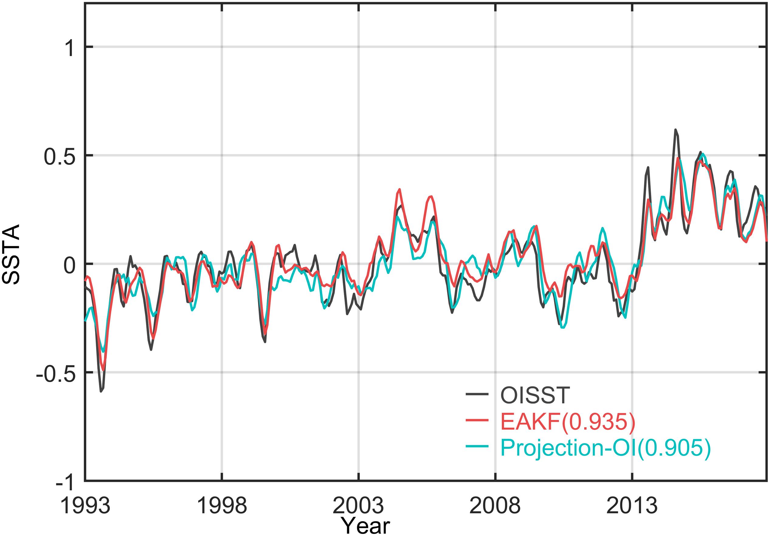
Figure 1. Time series of area-averaged SSTAs (units: °C) over the North Pacific (20–70°N, 110°E–100°W) with respect to climatology for 1993–2017. Three-month-running smoothing is applied. The black line represents SSTAs from OISST v2 observation; red and blue lines represent EAKF and Projection-OI assimilation results, respectively. The values in brackets are correlation coefficients between assimilation results and observation.
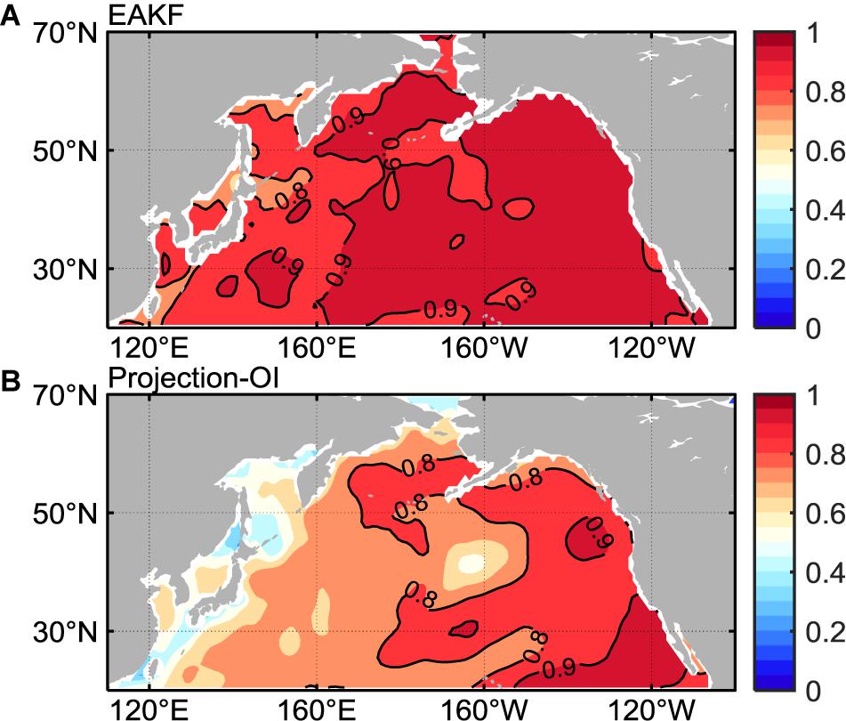
Figure 2. The anomaly correlation coefficient (ACC) of sea surface temperature (SST) between OISST v2 and assimilation results for 1993–2017. (A) EAKF; (B) Projection-OI. ACC is significantly greater than zero at the 95% confidence level. Only the 0.8 and 0.9 contours are plotted.
Surface observation data, including SST and SLA, were assimilated into FIO-ESM v1.0 using EAKF and Projection-OI assimilation schemes. The ocean subsurface layer is considerably changed under the data assimilation. Here, the difference between EAKF and observed temperatures was calculated to estimate the error of the EAKF scheme; similarly, the difference between Projection-OI and observed temperatures was calculated to estimate the error of the Projection-OI scheme:
where temperature changes refer to the difference between the absolute values of the errors of the two schemes; negative temperature changes indicate that the absolute difference between EAKF and observed temperatures is smaller than that between Projection-OI and observed temperatures. Figure 3 shows temperature changes along 45°N in the North Pacific. Negative temperature changes centered around 170–140°W from the surface to a depth of 300 m, and along the western coast at a depth of 100 m, indicating that EAKF is superior to Projection-OI in assimilating observed ocean temperatures for these locations. The EAKF and Projection-OI schemes use different projection methods to assimilate and project observed SST and SLA onto the subsurface vertical profile. The EAKF scheme uses the covariant relationship among different ensemble members, adjusting the temperature profile while also adjusting the current velocity coordinately, resulting in improved temperature simulation below the sea surface, which are superior to those obtained with the Projection-OI scheme. Distributions of subsurface negative temperature changes (centered around 170–140°W and 140–150°E in Figure 3) are consistent with that of high ACC skill (located in the central and western North Pacific as shown in Figure 2), indicating that the subsurface ocean temperature changes are directly associated with data assimilation techniques. Besides, this improvement is possible to be amplified via air–sea interaction in the coupled system. The improved SST, in turn, may derive inferior winds that contribute to better estimates of subsurface thermal conditions (Luo et al., 2005; Zhu et al., 2017a).
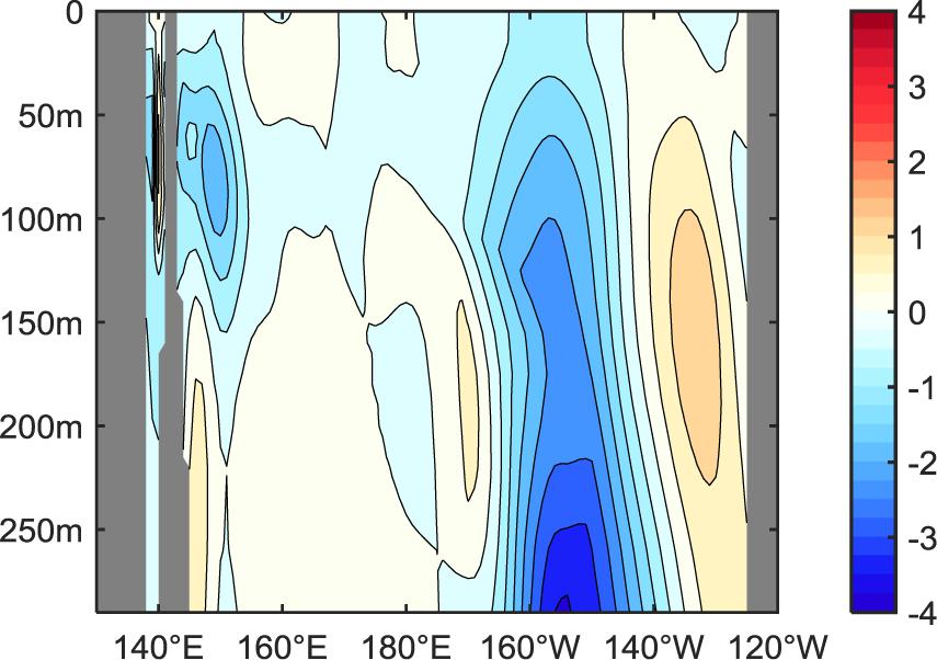
Figure 3. The ocean temperature changes along 45°N in the North Pacific as the EAKF scheme compared with the Projection-OI assimilation scheme. This change was calculated according to Eq. (4) for 1993–2017 (units: °C). The negative value indicates improvement with EAKF data assimilation.
Evaluation of Prediction Skill
Initialization of hindcasts with EAKF and Projection-OI data assimilation were conducted for 1993–2017. Figure 4 shows ACC of SST with lead times of 2, 4, and 6 months between OISST v2 dataset and hindcast results. We explore the impact of two different data assimilation schemes on the seasonal prediction skill for SST in the North Pacific. For lead times of 2, 4, and 6 months, the skill of FIO-ESM v1.0 to hindcast seasonal SST in the North Pacific is higher with EAKF data assimilation and lower with Projection-OI data assimilation. ACC at a 2-month lead time exceeds 0.5 over most of the North Pacific and is higher than 0.9 in the eastern Pacific. The prediction based on Projection-OI assimilation shows lower prediction skills with the ACC below 0.5 in most parts of North Pacific. As the lead time of prediction increases from 2 to 6 months, values of AAC gradually decreased. For lead times of 2, 4, and 6 months, the spacial distribution of ACCs indicates low skill in SST prediction over the KOE region where the active mesoscale processed combined with strong air-sea interactions is present. The remarkable predicted bias over the KOE region is consistent with results from previous research (Wen et al., 2012) and is a common problem in seasonal prediction over the North Pacific.
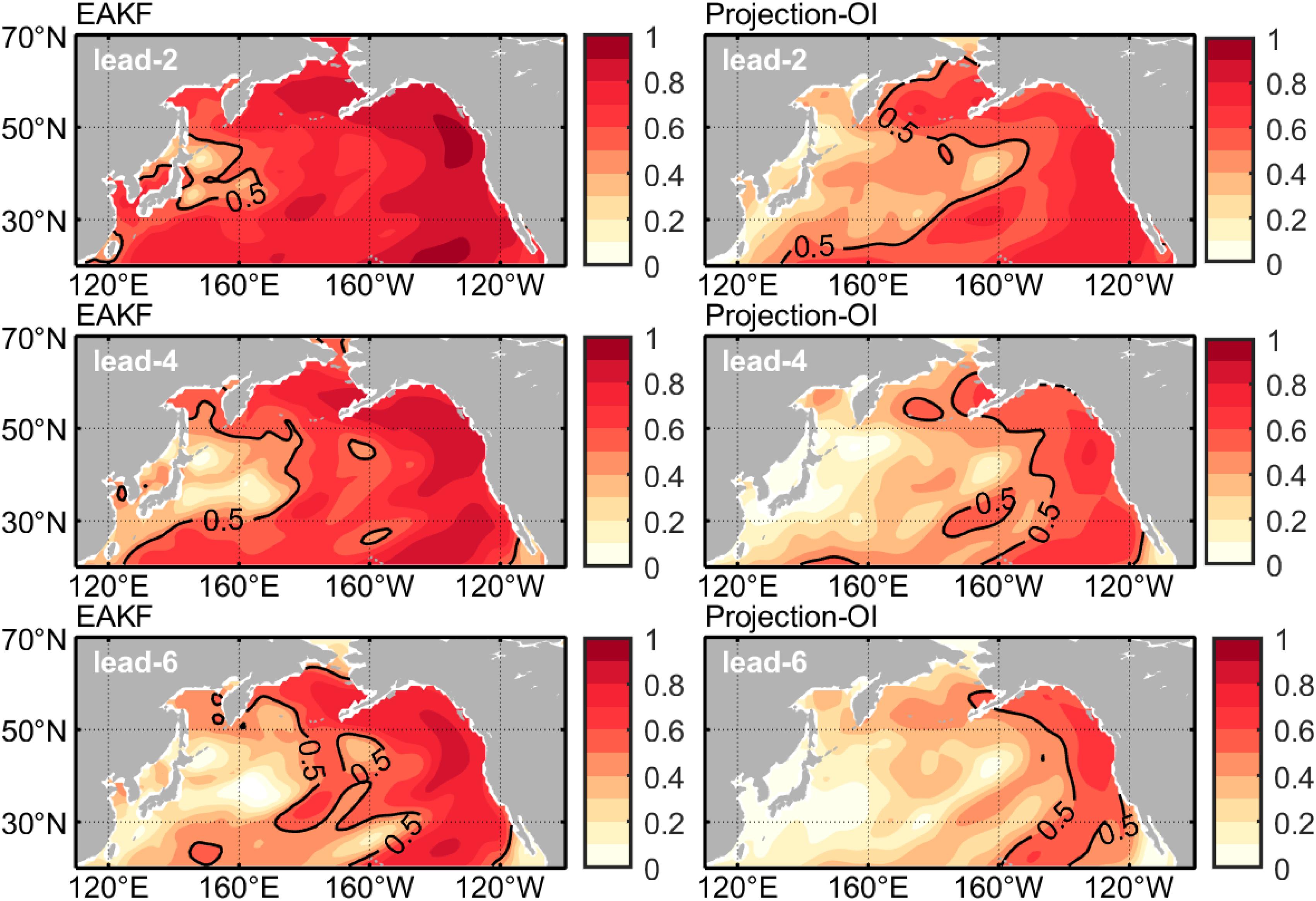
Figure 4. Distributions of ACC between IOSST v2 and hindcasts using the EAKF and Projection-OI data assimilation methods for the 2-, 4-, 6-months lead in the North Pacific. Only the line of the 0.5 contour is plotted.
To show the prediction skill initialized by two data assimilation methods more clearly, we examine the differences between ACC from EAKF and that from Projection-OI were calculated for each lead month. Figure 5 shows a clear difference over the Western central Pacific, particularly in the Okhotsk Sea, Japan Sea, and China Seas in the first lead month. Starting from a 2-month lead, large positive values are found in the Bering Sea and the Gulf of Alaska of the eastern North Pacific and extend along the northeast–southwest banded area in central Pacific. This positive value indicating improvement with EAKF method varies with increasing lead months and remaining in place for lead times of 5 and 6 months. Due to the coordinated adjustment at the surface and the entire water column in vertical in EAKF, SST hindcasts with EAKF data assimilation are superior to those with Projection-OI data assimilation. The difference between the two ACCs does not decrease with increasing lead time. Prediction skill strongly depends on initial conditions, and the dependence can last for lead times of up to two seasons.
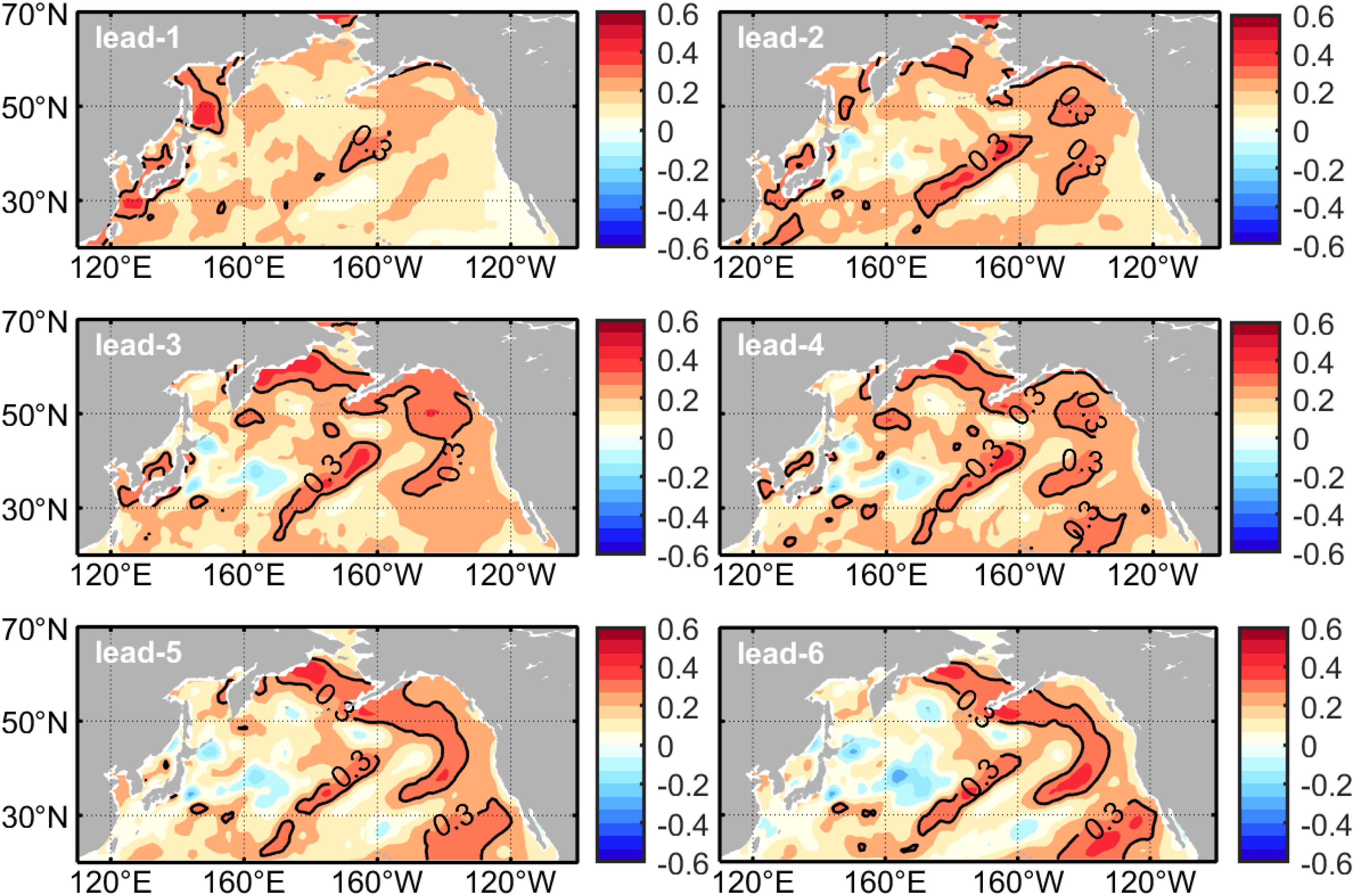
Figure 5. The differences of ACC between the EAKF and Projection-OI hindcasts in each lead month averaged for 1993–2017. Only the line of 0.3 contour is plotted.
The times series of area-averaged (30–50°N, 150°E–150°W) SSTAs differences between hindcast and OISST v2 for 1993–2017 for different lead times is shown in Figure 6. Biases of SSTAs from EAKF and from Projection-OI are similar, characterized by strong interannual variation. When the bias from the EAKF experiment is positive, there is also a positive bias in the Projection-OI prediction, and vice versa, indicating that the direction of prediction SST shifts is probably related to the model, regardless of which data assimilation method is used. However, the prediction bias initialized with Projection-OI is considerable larger than those from EAKF. The EAKF scheme performs better in restraining the shifts of model due to coordinated adjustment. Generally, the prediction bias for a lead time of 6 months is larger than biases for lead times of 2 or 4 months, either for EAKF or Projection-OI experiments.
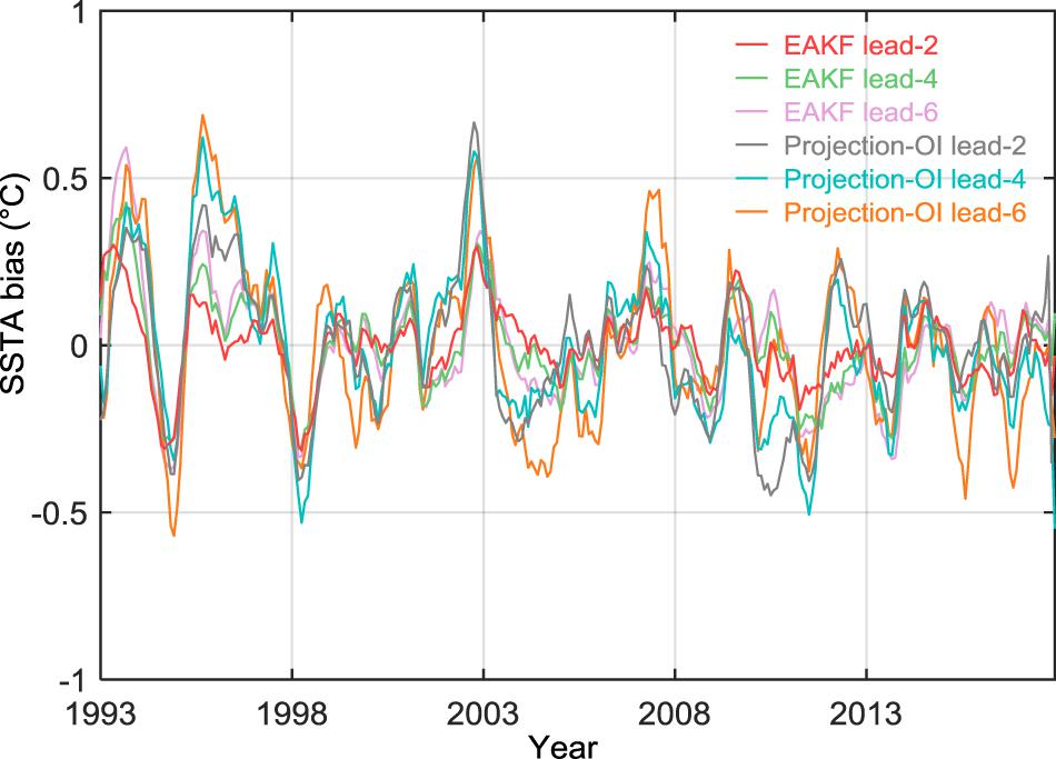
Figure 6. Time series of area-averaged SSTAs prediction biases over the North Pacific (30–50°N, 150°E–150°W; units: °C) with respect to OISST v2 for 1993–2017. The lines in different colors represent SSTA biases at the 2-, 4-, and 6-lead months in EAKF and Projection-OI predictions, respectively.
Seasonal dependence of prediction skill over the North Pacific was further investigated, and variation of ACC with horizontal axis of hindcast length and the vertical axis indicating the forecast starting month is shown in Figure 7. Hindcasts with EAKF data assimilation and that start from May are consistently high in skill, while the prediction skill is lower for hindcasts that start from November. The skill of Projection-OI hindcast is relatively low, but their ACC has the same characteristics of seasonal dependence as ACC of hindcasts with EAKF data assimilation. For both data assimilation schemes, hindcasts started from summer are lower in skill, which is consistent with the summer predictability barrier that is often encountered in short-term predictions. The differences show that the prediction skill is improved for all lead times by EAKF, especially for hindcasts that start in spring and autumn. The significant change with the differences exceeding 0.3 exists for lead times of 2–4 months. The FIO-ESM v1.0 with EAKF data assimilation tends to represent atmospheric and oceanic conditions relatively well and shows high skill of SST prediction over North Pacific.
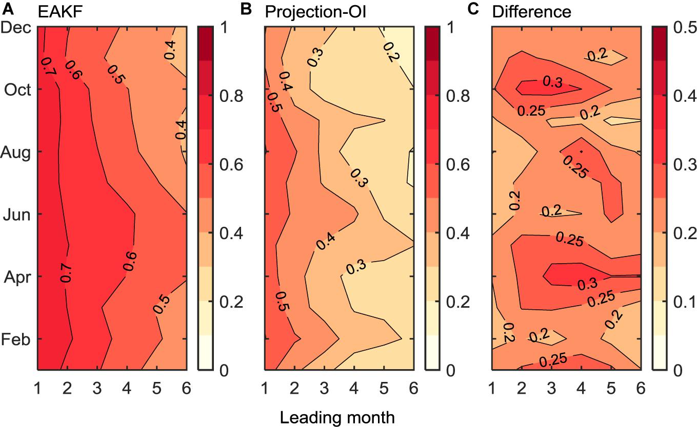
Figure 7. Evolution of area-averaged ACC over the North Pacific (20–70°N, 110°E–100°W); the horizontal axis represents the length of hindcasts, and the vertical axis indicates the starting month. (A) EAKF; (B) Projection-OI; and (C) EAKF–Projection-OI.
To explore the factors underlying the superior performance of hindcasts with EAKF data assimilation, temperature changes (as defined in Eq. 4) in the subsurface layer in the initial condition and difference of prediction skills between EAKF and Projection-OI hindcasts averaged for 1–6 lead months are illustrated in Figure 8. The significant improvement of prediction skill distributes in the banded area from 160°E to 160°W and in the high latitudes. Realistic initial conditions improve a model’s ability to capture climate variability and can improve the model’s skill to predict ENSO with a lead time of up to two seasons (Song et al., 2015). Signals from the tropics can have profound impacts on subtropical regions. Previous studies suggest that SSTA evolution in the North Pacific is strongly influenced by ENSO because of atmospheric teleconnections (Kim et al., 2015; Zhu et al., 2017a). The well-predicted ENSO can also improve skill to predict SSTA over the mid and high latitudes. In addition, we found that significant improvement of ocean temperature in the subsurface layer of the initial condition up to 3°C is shown to be located over the central North Pacific between 160°E and 160°W, which is generally in accordance with the region where the prediction skill is much improved. It reveals that the accurate subsurface structure in the initial condition could improve seasonal prediction skill in this region. However, more accurate ocean temperatures in the initial conditions are insufficient to remove all prediction errors, for example over the KOE region, characterized by active air–sea interactions and mesoscale processes.
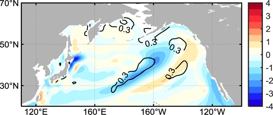
Figure 8. The temperature changes between EAKF and Projection-OI averaged at the 50–150 m vertical depth (shaded; units: °C) in the initial condition and the differences of ACC between the EAKF and Projection-OI hindcasts averaged in all lead months (contour, only 0.3 and 0.4 contours are plotted). The depth of 50–150 m covers the annual variation of mixed-layer depth.
Discussion
In this paper, the impacts of initial conditions on the skill of FIO-ESM v1.0 to predict seasonal SST over the North Pacific were assessed. Several assimilation and hindcast experiments for 1993–2017 were conducted using FIO-ESM v1.0 and the EAKF and Projection-OI data assimilation scheme. Evaluation of data assimilation output shows that simulated SST in the North Pacific from the EAKF scheme has a higher accuracy than that from Projection-OI runs. Seasonal SST variability in assimilation outputs is consistent with those in observations, with ACC exceeding 0.7 over most of the North Pacific. Both EAKF and Projection-OI assimilate the same surface observation data, however, the model with EAKF data assimilation has higher accuracy than that with Projection-OI in simulating subsurface ocean temperature.
Oceanic initial conditions play an important role in improving seasonal prediction skill. We analyzed hindcasts initialized by EAKF and Projection-OI data assimilation for the lead times of 1–6 months for 1993–2017. Prediction skill, as represented by ACC, is higher in hindcasts with EAKF than those with Projection-OI. ACC exceeding 0.5 is found over almost the entire North Pacific at a 2-month lead time and even over the eastern North Pacific at the 6-month leading time with EAKF initialization. Specifically, significant improvement of ACC distributes over the central North Pacific, as well as from the Bering Sea to the eastern North Pacific. Seasonal dependence of prediction skill was further assessed, and we found that, like other prediction systems, FIO-ESM v1.0 also encounters the North Pacific summer predictability barrier. EAKF can mitigate the prediction bias in contrast to Projection-OI for all lead times of 1–6 months, especially for the prediction starting from spring and autumn.
The prediction skill of FIO-ESM v1.0 over the KOE region is relatively low, because the complex dynamic environment with strong air–sea interaction in this region, which is difficult to parameterize correctly in climate models. Previous research suggested that the SST evolution and climate variability in extratropical Pacific are influenced by ENSO through atmospheric teleconnection and other associated dynamic processes (Hu et al., 2014). The skill to predict SSTAs in the central Pacific increases under ENSO remote forcing during the cold phase (Zhu et al., 2017a). If the model fails to simulate the teleconnection pattern, it may limit the prediction skill over the North Pacific (Kim et al., 2015). Realistic oceanic initial conditions improve ENSO predictions, which in turn have profound impacts on SSTAs predictions over the extratropical Pacific. In this study, we found that the EAKF data assimilation scheme improves the subsurface layer temperature in the initial condition and results in highly predicted ACC over the central North Pacific, indicating that accurate oceanic initial conditions, especially in the subsurface layer, can effectively improve prediction skill over the North Pacific. The projection method of the data assimilation scheme in the subsurface layer or deep waters can improve the prediction system’s performance. Development of short-term climate prediction systems has considerably improved seasonal prediction of SST over the North Pacific. For example, version 2 of the NCEP Climate Forecast System (CFSv21), which belongs to the new generation of operational climate forecast systems and has improved physics and increased resolution in the atmosphere–ocean–land coupled model. The skill of seasonal forecasts of 2-m temperatures over the United States from CFSv2 is nearly double of that from the old version of the prediction system. Global SST forecasts are also considerably improved with CFSv2 (Suranjana et al., 2014). Guan et al. (2014) show that the maximum skill based on CFSv2 hindcasts is confined in the tropical Pacific, and the prediction skill at the mid-latitudes of North Pacific remains low. Compared with CFSv2, FIO-ESM v1.0 exhibits improved prediction skills in the mid and high latitudes ocean. As shown in Figure 9, the zonal mean of ACCs (110°E–100°W) varies between 0.7 and 0.4 for 1- to 6-month lead (latitudes ranging from 35 to 50°N) in the EAKF experiment. Except for the influences of initial condition on prediction, it demonstrated that the physical process, such as wave effect, also plays a constructive role in climate prediction in North Pacific. To show the impacts of wave-induced mixing on seasonal prediction, the hindcast without waves is conducted using FIO-ESM v1.0 for 2016 (denoted as Exp.nowa), and the results were compared with the FIO-ESM v1.0 hindcast with EAKF data assimilation for 2016 (denoted as Exp.wave). Two experiments were started from each month of 2016 and initialized with the same initial conditions using the EAKF and ensemble method. When non-breaking wave-induced mixing effects are taken into account, the prediction bias of SSTAs is reduced by about 0.4°C for average lead times of 1–6 months at mid and high latitudes of the North Pacific (Figure 9B). Furthermore, bias reduction is found from the Okhotsk Sea across the mid-latitudes of the North Pacific (Figure 10) where low seasonal prediction skills have been persisting in other climate prediction systems. The prediction skill improvement due to surface wave exhibits seasonal dependence. Surface wave mixing has a stronger influence when the prediction starts in spring or early summer. As the prediction initiated from the second half of the year, ocean surface waves have little effect on prediction skill. The mixed-layer depth in the high latitude is shallow in summer, with the larger temperature gradient in the upper ocean. The enhanced vertical mixing bringing more cold water from the subsurface to the surface reduces SST. At low latitudes of the Pacific, the deep mixed-layer depth with weak wave-induced mixing results in a slight reduction in SST. In winter, the mixed-layer depth is deep, and the temperature gradient in the upper ocean is small. Due to the limitation of penetration depth, wave-induced mixing is unable to act on the water beneath the mixed layer. Furthermore, the decrease in the vertical diffusion coefficient reduces vertical water exchange, preventing downward heat transfer. As a result, upper ocean temperatures change little or even increase. The effect of surface wave on seasonal prediction of SST is more pronounced in summer, because of shallow mixed-layer depth (Zhao et al., 2019b). Seasonal predictions over the North Pacific over long lead times can be improved by incorporating realistic initial conditions produced by effective data assimilation schemes and reasonable physical processes in climate models.
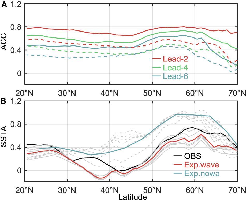
Figure 9. (A) Zonal mean ACC (110°E–100°W) between IOSST v2 datasets and hindcast results in EAKF (solid line) and Projection-OI (dashed line) runs. Red, green, and blue lines represent for 2-, 4-, 6-month lead, respectively. (B) Zonal mean SSTAs (110°E–100°W; units: °C) with respect to 1993–2017 climatology in observation (black), Exp.wave (red) and Exp.nowa (blue) mean averaged for 1–6 lead months, and gray solid and dashed lines represent the different lead month in Exp.wave and Exp.nowa.
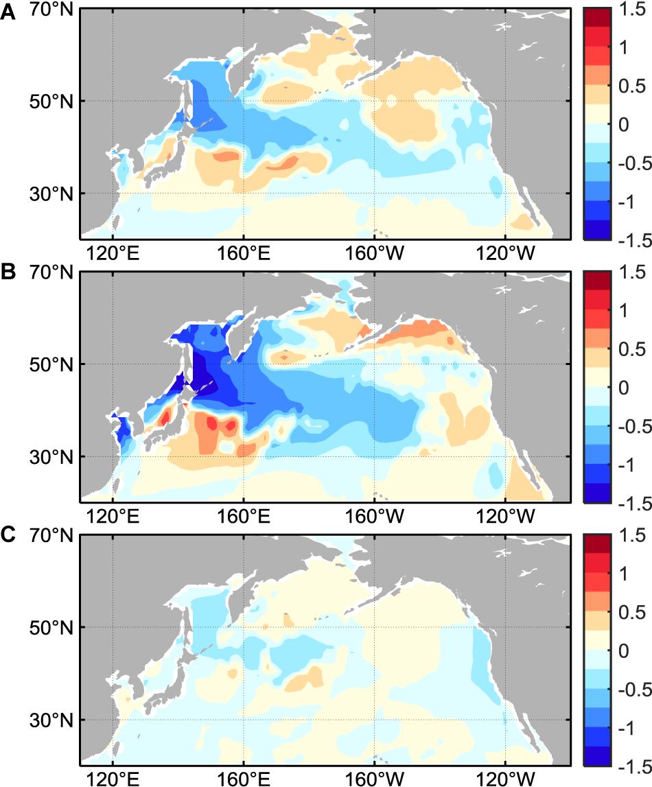
Figure 10. The differences of absolute predicted biases between Exp.wave and Exp.nowa in 2016. (A) Annual mean; (B) Jan-Jun mean; and (C) Jul-Dec mean. The hindcasts with or without wave are respectively compared with OISST v2 to show the predicted biases. Then the difference of absolute values of the biased between Exp.wave and Exp.nowa are calculated. As definited above, the negative value, indicating that the absolute difference between EAKF and observation is smaller than that between Projection-OI and OISST v2, represents the improvement due to the surface wave effects.
Data Availability Statement
The datasets of FIO-ESM v1.0 for this study can be found in: http://data.fio.org.cn/qiaofl/FIO-ESM-prediction.
Author Contributions
FQ initially designed and organized the whole analysis. YS conducted the hindcast experiments and made some figures and the first draft. YZ assisted in the analysis and improvement of the figures and manuscript. XY, YZ, and YB implemented the EAKF and Projection-OI data assimilation schemes into the FIO-ESM v1.0 and set up the short-term climate prediction system. All authors contributed to the writing of the manuscript.
Funding
This research was jointly supported by the National Key Research and Development Program of China (2017YFC1404004 and 2018YFC1506004), the International Cooperation Project of Indo-Pacific Ocean Environment Variation and Air–Sea Interactions (GASI-IPOVAI-06&05 and GASI-04-QYQH-01), and the National Natural Science Foundation of China (41821004 and 41676020).
Conflict of Interest
The authors declare that the research was conducted in the absence of any commercial or financial relationships that could be construed as a potential conflict of interest.
Acknowledgments
We thank the National Supercomputer Center in Tianjin for providing computing resource. All experiments were carried out at National Supercomputer Center in Tianjin, and the calculations were performed on TianHe-1(A).
Footnotes
References
Alessandri, A., Borrelli, A., Masina, S., Cherchi, A., Gualdi, S., Navarra, A., et al. (2010). The INGV-CMCC seasonal prediction system: improved ocean initial conditions. Mon. Weather Rev. 138, 2930–2952. doi: 10.1175/2010MWR3178.1
Alexander, M. A. (1999). The re-emergence of SST anomalies in the North Pacific Ocean. J. Clim. 12, 2419–2433. doi: 10.1175/1520-04421999012<2419:TROSAI<2.0.CO
Anderson, J. L. (2001). An Ensemble adjustment kalman filter for data assimilation. Mon. Weather Rev. 129, 2884–2903. doi: 10.1175/1520-04932001129<2884:AEAKFF<2.0.CO;2
Banzon, V., Smith, T. M., Chin, T. M., Liu, C., and Hankins, W. (2016). A long-term record of blended satellite and in situ sea-surface temperature for climate monitoring, modeling and environmental studies. Earth Syst. Sci. Data 8, 165–176. doi: 10.5194/essd-8-165-2016
Barnston, A., Tippett, M., Van den Dool, H., and Unger, D. (2015). Toward an improved multi-model ENSO prediction. J. Appl. Meteorol. Climatol. 54, 1579–1595. doi: 10.1175/JAMC-D-14-0188.1
Barnston, A. G., Glantz, M. H., and He, Y. (1999). Predictive skill of statistical and dynamical climate models in SST forecasts during the 1997/98 El Niño episode and the 1998 La Nifmars-07-00504a onset. Bull. Am. Meteorol. Soc. 80, 217–243. doi: 10.1175/1520-047719990802.0.CO;2
Bayr, T., Domeisen, D. I. V., and Wengel, C. (2019). The effect of the equatorial Pacific cold SST bias on simulated ENSO teleconnections to the North Pacific and California. Clim. Dyn. 53, 3771–3789. doi: 10.1007/s00382-019-04746-9
Bishop, C. H., Etherton, B. J., and Majumdar, S. J. (2001). Adaptive sampling with the ensemble transform kalman filter. Part I: Theor. Aspects. Mon. Weather Rev. 129, 420–436. doi: 10.1175/1520-049320011292.0.CO;2
Cane, M., Zebiak, A., and Dolan, S. C. (1986). Experimental forecasts of El Niño. Nature 321, 827–832. doi: 10.1038/321827a0
Chen, H., Yin, X., Bao, Y., and Qiao, F. (2015). Ocean satellite data assimilation experiments in FIO-ESM using ensemble adjustment Kalman filter. Scie. China: Earth Sci. 59, 484–494. doi: 10.1007/s11430-015-5187-2
Duan, W., and Wu, Y. (2014). Season-dependent predictability and error growth dynamics of Pacific Decadal Oscillation-related sea surface temperature anomalies. Clim. Dyn. 44, 1053–1072. doi: 10.1007/s00382-014-2364-5
Ducet, N., Traon, P., and Reverdin, G. (2000). Global high-resolution mapping of ocean circulation from TOPEX/Poseidon and ERS-1 and -2. J. Geophys. Res. Oceans 105, 19477–19498. doi: 10.1029/2000jc900063
Eddy, A. (1964). The objective analysis of horizontal wind divergence fields. Q. J. R. Meteorol. Soc. 90, 424–440. doi: 10.1002/qj.49709038606
Evensen, G. (1994). Sequential data assimilation with a nonlinear quasigeotropic model using Monte Carlo methods to forecast error statistics. J. Geophys. Res. 99, 143–162. doi: 10.1029/94jc00572
Ezer, T., and Mellor, G. (1997). Simulations of the Atlantic Ocean with a free surface sigma coordinate ocean model. J. Geophys. Res. Atmospheres 1021, 15647–15658. doi: 10.1029/97JC00984
Good, S. A., Martin, M. J., and Rayner, N. A. (2013). EN4: quality controlled ocean temperature and salinity profiles and monthly objective analyses with uncertainty estimates. J. Geophys. Res. Oceans 118, 6704–6716. doi: 10.1002/2013JC009067
Guan, Y., Zhu, J., Huang, B., Hu, Z. Z., and James, L. K. (2014). South Pacific Ocean dipole: a predictable mode on multiseasonal time scales. J. Clim. 27, 1648–1658. doi: 10.1175/jcli-d-13-00293.1
Hu, Z., Kumar, A., Huang, B., Zhu, J., and Guan, Y. (2014). Prediction Skill of North pacific variability in NCEP climate forecast system Version 2: impact of ENSO and Beyond. J. Clim. 27, 4263–4272. doi: 10.1175/JCLI-D-13-00633.1
Jacox, M. G., Alexander, M. A., Stock, C. A., and Hervieux, G. (2019). On the skill of seasonal sea surface temperature forecasts in the California Current System and its connection to ENSO variability. Clim. Dyn. 53, 7519–7533. doi: 10.1007/s00382-017-3608-y
Jones, R. H. (1965). Optimal estimation of initial conditions for numerical prediction. J. Atmos. Sci. 22, 658–663. doi: 10.1175/1520-046919650222.0.CO;2
Kim, H., Webster, P. J., and Curry, J. A. (2012). Seasonal prediction skill of ECMWF System 4 and NCEP CFSv2 retrospective forecast for the Northern Hemisphere Winter. Clim. Dyn. 39, 2957–2973. doi: 10.1007/s00382-012-1364-6
Kim, S., Jeong, H., and Jin, F. (2017). Mean bias in seasonal forecast model and ENSO prediction error. Sci. Rep. 7:6029. doi: 10.1038/s41598-017-05221-3
Kim, S., Kim, H., Min, S., Son, H., Won, D., Jung, H., et al. (2015). Intra-winter atmospheric circulation changes over East Asia and North Pacific associated with ENSO in a seasonal prediction model. Asia Pacific J. Atmospheric Sci. 51, 49–60. doi: 10.1007/s13143-014-0059-9
Kug, J. S., Kang, I., and Choi, D. (2008). Seasonal climate predictability with Tier-one and Tier-two prediction systems. Clim. Dyn. 31, 403–416. doi: 10.1007/s00382-007-0264-7
Kumar, A., Jha, B., and Wang, H. (2014). Attribution of SST variability in global oceans and the role of ENSO. Clim. Dyn. 43, 209–220. doi: 10.1007/s00382-013-1865-y
Lau, K. M., Lee, J., Kim, K., and Kang, I. (2004). The North pacific as a regulator of summertime climate over eurasia and North America. J. Clim. 17, 819–833. doi: 10.1175/1520-04422004017<0819:tnpaar<2.0.co;2
Liu, Y., and Ren, H. (2017). Improving ENSO prediction in CFSv2 with an analogue-based correction method. Int. J. Climatol. 37, 5035–5046. doi: 10.1002/joc.5142
Liu, Z., and Alexander, M. (2007). Atmospheric bridge, oceanic tunnel, and global climatic teleconnections. Rev. Geophys. 45:RG2005. doi: 10.1029/2005RG000172
Lorenz, E. N. (1969). Atmospheric predictability as revealed by naturally occurring analogues. J. Atmos. Sci. 26, 636–646. doi: 10.1175/1520-04691969262.0.CO;2
Luo, J., Masson, S., Behera, S., Shingu, S., and Yamagata, T. (2005). Seasonal Climate Predictability in a Coupled OAGCM Using a Different Approach for Ensemble Forecasts. J. Clim. 18, 4474–4497. doi: 10.1175/JCLI3526.1
Qiao, F., Song, Z., Bao, Y., Song, Y., Shu, Q., Huang, C., et al. (2013). Development and evaluation of an Earth system model with surface gravity waves. J. Geophys. Res. Oceans 118, 4514–4524. doi: 10.1002/jgrc.20327
Qiao, F., Yuan, Y., Ezer, T., Xia, C., Yang, Y., Lü, X., et al. (2010). A three-dimensional surface wave-ocean circulation coupled model and its initial testing. Ocean Dynamics 60, 1339–1355. doi: 10.1007/s10236-010-0326-y
Qiao, F., Yuan, Y., Yang, Y., Zheng, Q., Xia, C., and Ma, J. (2004). Wave-induced mixing in the upper ocean: distribution and application to a global ocean circulation model. Geophys. Res. Lett. 31, 293–317. doi: 10.1029/2004GL019824
Ratheesh, S., Sharma, R., and Basu, S. (2012). Projection-based assimilation of satellite-derived surface data in an indian ocean circulation model. Mar. Geodesy 35, 175–187. doi: 10.1080/01490419.2011.637855
Reynolds, R. W., Smith, T. M., Liu, C., Chelton, D. B., Casey, K. S., and Schlax, M. G. (2007). Daily high-resolution-blended analyses for sea surface temperature. J. Clim. 20, 5473–5496. doi: 10.1175/2007JCLI1824.1
Rosati, A., Miyakoda, K., and Gudgel, R. (1997). The impact of ocean initial conditions on ENSO forecasting with a coupled model. Mon. Weather Rev. 125, 754–772. doi: 10.1175/1520-04931997125<0754:TIOOIC<2.0.CO;2
Song, Z., Shu, Q., Bao, Y., Yin, X., and Qiao, F. (2015). The prediction on the 2015/16 El Niño event from the perspective of FIO-ESM. Acta Oceanol. Sin. 34, 67–71. doi: 10.1007/s13131-015-0787-4
Suranjana, S., Shrinivas, M., Wu, X., Wang, J., Nadiga, S., Tripp, P., et al. (2014). The NCEP climate forecast system version 2. J. Clim. 27, 2185–2208. doi: 10.1175/jcli-d-12-00823.1
Wang, C., Zhang, L., Lee, S., Wu, L., and Mechoso, C. R. (2014). A global perspective on CMIP5 climate model biases. Nat. Clim. Change 4, 201–205. doi: 10.1038/nclimate2118
Wen, C., Xue, Y., and Kumar, A. (2012). Seasonal Prediction of North Pacific SSTs and PDO in the NCEP CFS Hindcasts. J. Clim. 25, 5689–5710. doi: 10.1175/JCLI-D-11-00556.1
Wu, Y., Duan, W., and Rong, X. (2016). Seasonal predictability of sea surface temperature anomalies over the kuroshio-oyashio extension: low in summer and high in winter. J. Geophys. Res. Oceans 121, 6862–6873. doi: 10.1002/2016JC011887
Yin, X., Qiao, F., Xia, C., Lü, X., and Yang, Y. (2010). Reconstruction of eddies by assimilating satellite altimeter data into Princeton Ocean Model. Acta Oceanol. Sin. 29, 1–11. doi: 10.1007/s13131-010-0001-7
Zhao, X., Li, J., and Zhang, W. (2012). Summer persistence barrier of sea surface temperature anomalies in the Central Western North Pacific. Adv. Atmospheric Sci. 29, 1159–1173. doi: 10.1007/s00376-012-1253-2
Zhao, Y., Yin, X., Song, Y., and Qiao, F. (2019a). Seasonal prediction skills of FIO-ESM for North Pacific Sea surface temperature and precipitation. Acta Oceanol. Sin. 38, 5–12. doi: 10.1007/s13131-019-1366-x
Zhao, Y., Yin, X., Song, Y., and Qiao, F. (2019b). Effect of wave-induced mixing on sea surface temperature seasonal prediction in the North Pacific in 2016. Haiyang Xuebao 41, 52–61. doi: 10.3969/j.issn.0253-4193.2019.03.006
Zheng, F., and Zhu, J. (2010). Spring predictability barrier of ENSO events from the perspective of an ensemble prediction system. Global Planet. Change 72, 108–117. doi: 10.1016/j.gloplacha.2010.01.021
Zhu, J., Huang, B., Balmaseda, M. A., Kinter, J. L., Peng, P., Hu, Z., et al. (2013). Improved reliability of ENSO hindcasts with multi-ocean analyses ensemble initialization. Clim. Dyn. 41, 2785–2795. doi: 10.1007/s00382-013-1965-8
Zhu, J., Huang, B., Marx, L., Kinter, J. L., Balmaseda, M. A., Zhang, R., et al. (2012). Ensemble enso hindcasts initialized from multiple ocean analyses. Geophys. Res. Lett. 39:L09602. doi: 10.1029/2012GL051503
Zhu, J., Kumar, A., Lee, H. C., and Wang, H. (2017a). Seasonal predictions using a simple ocean initialization scheme. Clim. Dyn. 49, 3989–4007. doi: 10.1007/s00382-017-3556-6
Keywords: seasonal prediction skill, FIO-ESM, North Pacific, ensemble adjustment kalman filter, assimilation scheme, sea surface temperature
Citation: Song Y, Zhao Y, Yin X, Bao Y and Qiao F (2020) Evaluation of FIO-ESM v1.0 Seasonal Prediction Skills Over the North Pacific. Front. Mar. Sci. 7:504. doi: 10.3389/fmars.2020.00504
Received: 31 March 2020; Accepted: 03 June 2020;
Published: 24 July 2020.
Edited by:
Shoshiro Minobe, Hokkaido University, JapanReviewed by:
Adam Thomas Devlin, The Chinese University of Hong Kong, ChinaJieshun Zhu, University of Maryland, United States
Copyright © 2020 Song, Zhao, Yin, Bao and Qiao. This is an open-access article distributed under the terms of the Creative Commons Attribution License (CC BY). The use, distribution or reproduction in other forums is permitted, provided the original author(s) and the copyright owner(s) are credited and that the original publication in this journal is cited, in accordance with accepted academic practice. No use, distribution or reproduction is permitted which does not comply with these terms.
*Correspondence: Fangli Qiao, cWlhb2ZsQGZpby5vcmcuY24=
 Yajuan Song
 Yiding Zhao
 Xunqiang Yin1,2,4
 Ying Bao
 Fangli Qiao