A Water Mass Classification Approach to Tracking Variability in the East Australian Current

The East Australian Current (EAC) is a southward flowing western boundary current that transports relatively warm and nutrient-depleted subtropical water along Australia's east coast. The EAC is a highly variable system that is formed by temporally-varying mixtures of water in the Coral Sea that do not form a linear density gradient or conform to a set range of temperature and salinity values. It can therefore be difficult to track EAC dynamics across both space and time using traditional analytical approaches. In order to more accurately quantify variability and trends in penetration of the EAC we develop a novel machine-learning classification approach to quantify variability in coastal EAC dynamics along a latitudinal gradient within the EAC extension zone in southeastern Australia. Applying our method to data from a 22-year free running regional hydrodynamic model revealed significant decadal-scale changes to EAC dynamics in the region. The annual period (generally in the austral summer) when the EAC is the dominant water mass in the region increased by approximately 2 months over the model time series. The encroachment of the EAC's traditional period of summer dominance into winter may have significant ecological implications through the acceleration of poleward range extensions by vagrant tropical species, facilitation of community phase shifts from temperate to tropical assemblages, and a phenological shift in the timing of major phytoplankton blooms. These results highlight the need to further understand the rapid changes occurring within western boundary current systems, and illustrates how classification approaches may assist in uncovering patterns in these highly variable systems.

1. Introduction

Western boundary currents are strong and persistent features of ocean circulation that form along the western margins of the world's major ocean basins (Hogg and Johns, 1995; Imawaki et al., 2013). Primarily generated by wind-driven anticyclonic subtropical gyres, these currents play a key role in meridional heat transport and climate regulation through the transportation of warm subtropical waters from low to high latitudes (Yu and Weller, 2007). Due to baroclinic instabilities, western boundary currents have characteristically elevated levels of eddy kinetic energy (Archer et al., 2018). As a consequence, western boundary currents are typically highly variable and dynamic, making it difficult to track these systems through time.

The East Australian Current (EAC) is a southward flowing western boundary current that transports relatively warm and nutrient-depleted subtropical water from the Coral Sea along Australia's east coast (Suthers et al., 2011). The current separates from the coast between 31 and 33°S to form the eastward-flowing Tasman Front and a poleward propagating eddy field called the EAC extension (Cetina-Heredia et al., 2014) (Figure 1). The current has intensified over the last eight decades with strong lines of evidence demonstrating a marked increase in the strength, duration, and frequency of southward incursions of EAC water (Ridgway, 2007; Johnson et al., 2011). These patterns are consistent with a “spin up” of the South Pacific sub-tropical gyre (Cai et al., 2005; Cai, 2006). Modeling suggests that this intensification is not spatially uniform. The main EAC transport volume is projected to vary little, increasing by only 0.7% (0.2 Sv) between 1990 and 2060, while the transport of the EAC extension is predicted to increase by ~40% (4.3 Sv) over the same period (Oliver and Holbrook, 2014). This intensification has resulted in the EAC extension zone seeing rates of ocean warming that are 3–4 times the global average, making southeast Australia one of the fastest warming regions in the southern hemisphere (Wu et al., 2012).

FIGURE 1

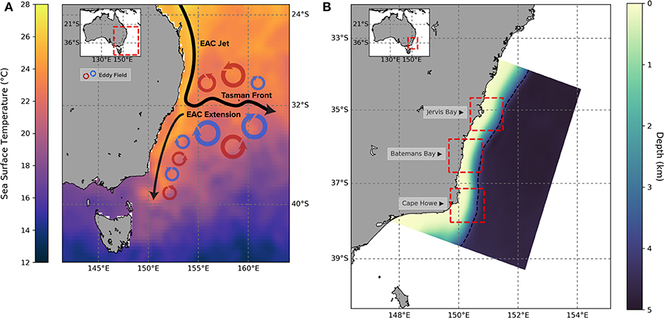
Figure 1. (A) A simplified schematic of the East Australian Current (EAC) showing the primary features and eddy fields. The schema is overlaid over mean SST for the 10th of December, 2000—provided by NOAA (https://psl.noaa.gov/data/gridded/data.noaa.oisst.v2.highres.html) (Reynolds et al., 2007) and; (B) Map of the study region in southeastern Australia showing the extent of the hydrodynamic data-subset used in the analysis, with bathymetry overlaid. The three marine ecosystem study sites are shown as red boxes. Only the regions within the boxes between the coast and the 4,000 m bathymetric contour line (black dotted line) were analyzed.

The effects of EAC intensification on coastal marine systems in southeastern Australia are already evident (Suthers et al., 2011). For example: the modification of nutrient loading regimes (Harris et al., 1987, 1991); unprecedented, prolonged marine heatwaves (Oliver et al., 2017); shifts in planktonic species assemblages and abundances (Thompson et al., 2009; Johnson et al., 2011; Kelly et al., 2016; Larsson et al., 2018); changes in coastal connectivity for larvae (Roughan et al., 2011; Cetina-Heredia et al., 2015); the migration of typically subtropical species poleward (Edyvane, 2003; Pittock, 2003; Thresher et al., 2003; Johnson et al., 2011; Mos et al., 2017); shifts in the distribution of pelagic fishes (Hobday et al., 2011); and changes to marine predator foraging behavior (Carroll et al., 2016, 2017; Phillips et al., 2019). Consequently there is a need to further understand variability in the EAC, how this variability is changing through time, and subsequently how these changes may impact living systems.

Like other western boundary currents, the EAC is driven by a variable field of mesoscale eddies (Brassington et al., 2011) that typically migrate poleward along the coast. The movement of these eddies can be further complicated by reabsorption into the EAC (Nilsson and Cresswell, 1980), coalescence of one or more eddies (Cresswell, 1982), or injections of filaments of surrounding water into the eddy (Cresswell, 1983) and surface flooding (Baird et al., 2011). As a consequence, the flow patterns of the East Australian Current are so complex that often a single continuous current cannot be identified (Godfrey et al., 1980). Despite this complexity, patterns have been observed in the EAC at seasonal, inter-annual and decadal scales (Ridgway et al., 2008). Seasonally, the EAC jet strengthens in the summer and has a weaker flow during winter (Archer et al., 2017) while inter-annually, the El Niñ~o–Southern Oscillation (ENSO) is correlated with the temporal fluctuations of the latitude at which the EAC separates from the continent and moves offshore as the Tasman Front (Cetina-Heredia et al., 2014). Additionally, a “quasi-decadal” pattern is evident in the maxima and minima of the southward penetration of the EAC extension (Ridgway, 2007).

The EAC is challenging to study as the current does not conform to linear mixing models (Tilburg et al., 2001; Bull et al., 2017) due to being formed by temporally-varying mixtures of water masses in the Coral-Sea (Ridgway and Dunn, 2003). Because the water mass does not typically form a linear density gradient or conform to a set range of temperature and salinity values, it can be difficult to determine when a given region is experiencing flow originating predominately from the EAC or from other regions.

Machine learning is a tool that can be leveraged to classify dynamic and complex features in oceanic systems (Jones et al., 2014; Gangopadhyay et al., 2015). Machine learning algorithms are designed to learn from one dataset (training set) to make predictions about a new, independent dataset (testing set) and are well suited to analysing big datasets common in oceanographic studies. Multiple machine learning techniques are available to approach classification problems (Weiss and Kulikowski, 1991; Kotsiantis, 2007) including logistic regression which is a particularly well suited tool to model the outcomes of categorical dependent variables (Hosmer et al., 2013) such as the presence/absence of ocean currents.

This study describes variability in EAC dynamics along a latitudinal gradient within the EAC extension, downstream of its typical separation zone, along southerneastern Australia. This is achieved through the development of a novel logistic regression classification algorithm that can identify water as being either subtropical origin (STO) or Tasman Sea origin (TSO). Classification is based on the surface temperature and salinity signatures of the two primary water masses known to influence our study region as proxies for EAC presence/absence. We then apply the classification algorithm to the output of a 22-year regional hydrodynamic model (Kerry and Roughan, 2020a) to examine variability and trends in EAC influence through time. We aim to provide a more detailed description of seasonal and inter-annual EAC dynamics, as well as describing spatial and temporal patterns of intensification in one of the fastest warming regions in the Southern Hemisphere. Our approach offers a framework to analyse variability in water mass influence that can be applied to other ocean systems.

2. Methods

2.1. Study Region

To assess latitudinal variability in EAC dynamics along Australia's east coast, we analyzed variability in EAC presence for three zones (100 km squares) centered on coastal marine park ecosystems: (i) Jervis Bay Marine Park (35.114°S, 150.95°E); (ii) Batemans Marine Park (36.227°S, 150.23°E); and (iii) Cape Howe Marine Park (37.587°S, 150.29°E) (Figure 1). These locations were selected as they each encompass coastal ecosystems of conservation concern that lie in the path of the EAC extension. Each study site was restricted to the area between the coastal boundary and the 4,000 m depth contour.

2.2. Data

The classification algorithm utilized surface temperature and salinity data from two sources: (i) the “CSIRO Atlas of Regional Seas” (CARS) (Ridgway et al., 2015) as the training set and; (ii) a custom configuration of the “Regional Ocean Modeling System” (ROMS 3.4) for circulation along the southeast coast of Australia (Kerry and Roughan, 2020b) as the testing set.

The CARS dataset is an atlas of ocean water properties derived from a quality-controlled archive of ocean measurements taken from research vessel instrument profiles and Argo floats from 1985 to 2009. These measurements are gridded at a 0.5 degree grid spatial resolution and averaged through time to provide a daily climatology of ocean conditions for each grid cell (Ridgway et al., 2002).

ROMS is a free-surface, hydrostatic, primitive equation ocean model solved on a curvilinear grid with a terrain following a vertical coordinate system (Shchepetkin and McWilliams, 2003, 2005). Time-stamped surface temperature and salinity data at a horizontal spatial resolution of ~2 km were extracted from a configuration of ROMS that produces a high resolution free running simulation of the EAC region (Kerry and Roughan, 2020a). Data were extracted for the period from 1994 to mid 2016. The BlueLink Reanalysis (BRAN3p5) (Oke et al., 2008) is used for the EAC-ROMS model initial conditions and boundary forcing over the 22-year period. EAC-ROMS has been validated against satellite and in situ observations to confirm that it resolves the mean dynamic features of the EAC including surface and subsurface variability, seasonality, and to ensure that it contains no net temperature drift (Kerry and Roughan, 2020a). For a full description of the EAC-ROMS specifications, parameters, and validation (see Kerry and Roughan, 2020a,b).

2.3. Algorithm Construction and Analysis

To quantify variability in EAC dynamics for each of the study sites, a supervised machine-learning classification algorithm was developed to assess the probability of surface water from the ROMS model output as being of either subtropical origin (STO) or Tasman Sea origin (TSO) based on the surface temperature and salinity signatures as a proxy for EAC-derived/non-EAC derived water. To do this, we undertook the following steps (Figure 2):

FIGURE 2

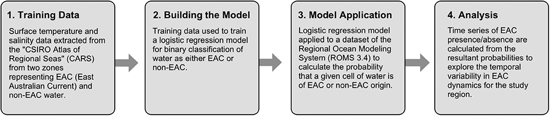
Figure 2. Schematic of the classification algorithm construction process.

(1) The classification algorithm was trained to identify STO and TSO surface waters using the CARS dataset. Data was extracted from two regional zones within the CARS dataset, selected to represent STO and TSO water (Figure 3). These regions were selected to be representative of the two primary water masses that are known to influence the study region: (A) Coral Sea (STO/EAC) and; (B) Tasman Sea (TSO/non-EAC) waters. Variables extracted from the CARS data set included temperature, salinity and “day of year” (DoY) to account for seasonal variability in water mass characteristics. A total of 58,765 data points were used to train the classification algorithm to identify the two water masses, based on time-varying patterns in their surface temperature and salinity profiles.

FIGURE 3

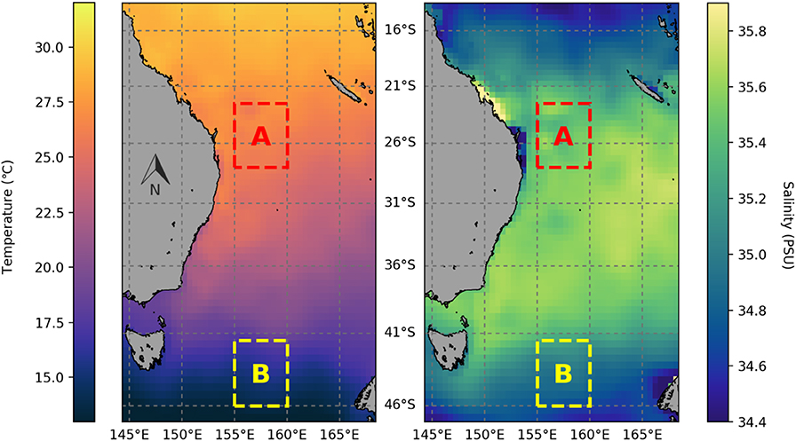
Figure 3. Example of data from the “CSIRO Atlas of Regional Seas” (CARS) showing surface temperature (°C) (left) and Salinity (PSU) (right) for the east coast of Australia. The mean state for the 15th day of February is shown as an example. These data were used to train the logistic regression model for the classification algorithm with box “A” representing the region used to train subtropical origin (STO) water and box “B” representing the region used to train Tasman Sea origin (TSO) water.

(2) The training dataset was then used to fit a logistic regression model to classify water as either STO or TSO. To test how well the model classified unseen portions of the CARS data, the performance of the model was tested using k-fold cross-validation (k = 10). This was achieved by randomly partitioning the training dataset into ten equal sized subsamples, using nine of these subsamples to train the model, and holding the remaining one out as a validation set to determine the accuracy of predictions. This process was then repeated ten times such that each of the subsamples was used once as the validation set. The results of this validation were then averaged to produce an estimation of the model's performance on the CARS data set.

(3) The logistic regression model was then applied to the ROMS model output. The probability of a given cell of water being STO was then calculated by applying the inverse logit function to the log-odds model predictions.

(4) A metric called the “classification ratio” was then calculated from the probability values to explore temporal variability in regional EAC influence, and was defined as the proportion of grid cells in a region classified as STO (probability >= 0.5) vs. TSO (probability < 0.5) for each day.

All code was developed with the general purpose programming language “Python” (Rossum, 1995) using the open-source machine learning software library “scikit-learn” (Pedregosa et al., 2011).

3. Results

The classification algorithm produced a metric of EAC presence for the study region and was able to track structural features such as EAC-derived eddies that were evident in the surface temperature and salinity profiles (Figure 4 and Video 1). Model evaluation using k-folds cross-validation on the CARS training data set indicated an accuracy of 99.91%. The method revealed latitudinal variability in the dynamics of the EAC extension, with differences being detected between the three study sites.

FIGURE 4

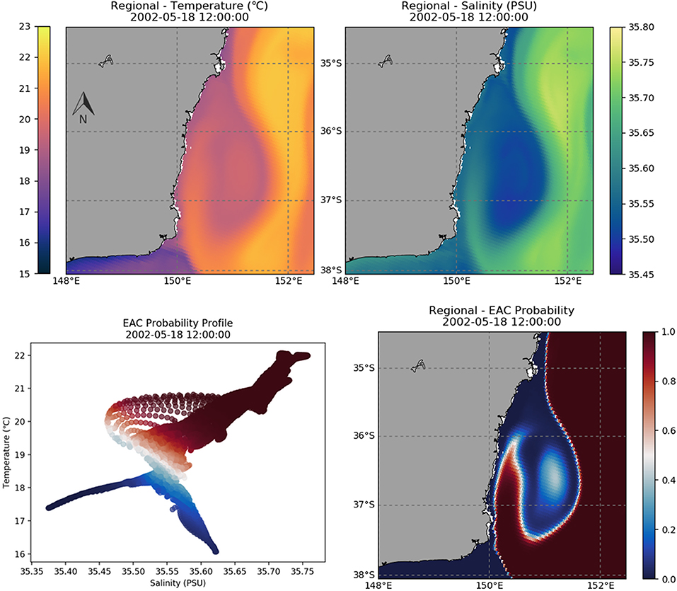
Figure 4. Example output of the East Australian Current (EAC) classification algorithm for the 18th of May, 2002. The top panels show temperature (left) and salinity (right) inputs from the ROMS dataset. The bottom right panel shows the EAC probability for the region calculated using the logistic regression algorithm, with a probability < 0.5 being classed as non-EAC and >= 0.5 classed as EAC. The bottom left panel shows the temperature salinity profile of model-predicted EAC water at the given time-step. An animation of these plots for the full 22 year model run can be viewed here: https://youtu.be/RczXvkWd420.

The monthly means of the “classification ratio” (ratio of STO to TSO water) demonstrate a sinusoidal seasonal cycle of EAC presence for the three study sites (Figure 5). Furthermore, the annual means of the “classification ratio” demonstrate a positive trend in the ratio of STO water for all three study sites over the 22-year model run. Each study site is characterized by different patterns of EAC dynamics, with mean period of STO dominance (period of time where the classification ratio is >0.5) being 246, 207, and 184 days for Jervis Bay, Batemans Bay, and Cape Howe, respectively (Figure 6). These patterns also appear to have changed over the study period. When comparing the first and last five years of the dataset, it is apparent that the period of EAC dominance is beginning earlier, persisting longer and ending later for all three study sites (Figure 6).

FIGURE 5

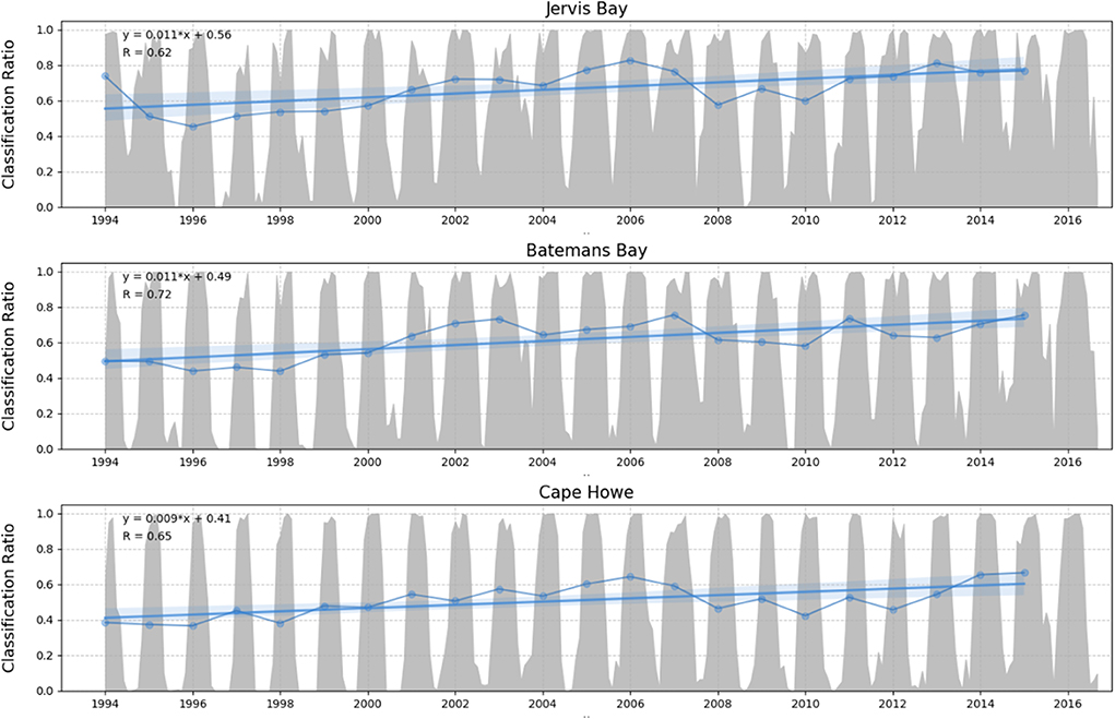
Figure 5. Plot showing the seasonal and inter-annual dynamics of East Australian Current (EAC) presence for each study site over the entire study period (1994–2016). The y-axis depicts the “classification ratio” which is the proportion of a study site's grid cells that were classified as being of subtropical origin (STO) to those classified as Tasman Sea origin (TSO) derived water. The shaded gray area represents the monthly means of the classification ratio. To investigate the inter-annual trend in EAC dynamics without seasonality, the yearly means are shown as blue points with a linear regression line (with a 95% confidence interval) and associated formula shown in the top left of each panel. The yearly mean for 2016 was excluded from analysis as data does not cover the full year.

FIGURE 6

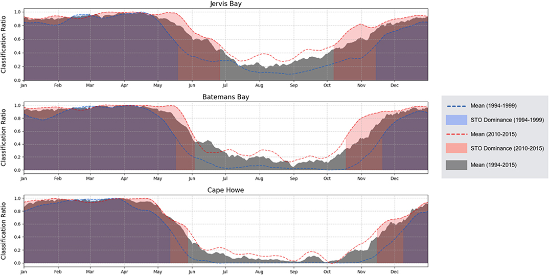
Figure 6. Figure showing the typical seasonal cycle of East Australian Current (EAC) presence for each study site for each day of the year. The y-axis depicts the “classification ratio” which is the proportion of a study site's grid cells that were classified as being subtropical origin (STO) water to those classified as Tasman Sea origin (TSO) water. The gray shaded area represents the mean seasonal cycle for each day of the year for the entire study period (1994–2016). The dashed lines show the mean seasonal cycle for each day of the year after the application of a Savitzky–Golay smoothing function (window length = 35, polynomial order = 3) for the first 5 years of the dataset (blue = 1994/01/01 to 1999/12/31) and last full 5 years of the data set (red = 2010/01/01 to 2015/12/31) with the respective colored shaded areas indicating the season when the classification ratio is >0.5 (period when the STO water is dominant).

For Jervis Bay the period of EAC dominance has increased by 75 days from 189 to 264 days and is now beginning almost a month earlier and persisting nearly a month later into June. At Batemans Bay the period of EAC dominance has increased by 50 days from 178 to 228 and is now beginning over a month earlier in late October and also persisting for half a month longer. At Cape Howe the period of EAC dominance has increased by 40 days from 156 to 196 days and now begins approximately one month earlier in mid November and ends half a month later at the end of May.

4. Discussion

The goal of this study was to produce a metric of East Australian Current (EAC) presence to assess seasonal and inter-annual patterns of EAC penetration within the EAC extension. This was achieved by developing a supervised machine learning logistic regression algorithm to classify water as either: (A) Sub-tropical origin (STO), representing EAC source water; or (B) Tasman Sea origin (TSO), representing non-EAC water; based on time-varying surface temperature and salinity profiles. The method was able to differentiate spatially complex features of the EAC such as eddies and filaments (Figure 4) and identified previously reported patterns of EAC dynamics within the EAC extension, such as a sinusoidal seasonal cycle (Cresswell, 2000), and a trend of intensification over the past 22 years (Ridgway, 2007). In addition, major spatially-explicit changes in the seasonal cycle of EAC dominance were identified at all three study sites across a 3.5 degree latitudinal gradient of the southeast Australian coastline.

Temporal dynamics of the EAC that were identified using the classification algorithm approach are consistent with that of previous research. The algorithm detected a sinusoidal seasonal cycle in EAC presence for each of the three study sites, with the EAC having a stronger presence in the summer months and a weaker influence during the winter (Ridgway and Godfrey, 1997; Cresswell, 2000). The seasonal cycle of EAC dynamics was found to vary with latitude, with each study site exhibiting different periods of EAC dominance (period of time where the EAC classification ratio was > 0.5). The study sites at more northerly latitudes had a greater mean period of EAC dominance (Figure 6). This was expected as the more northerly sites are closer to the EAC's separation latitude (between 31 and 33°S) where the majority of the EAC veers eastward as the Tasman Front and the extension zone begins (Cetina-Heredia et al., 2014). Consequently, more northerly sites will be the first to be exposed to the EAC as it penetrates southward during summer, and the last to be exposed as it retreats northward in the winter (Suthers et al., 2011).

Our algorithm also detected a positive inter-annual trend in EAC influence at each of the three study sites between 1994 and 2016 (Figure 5). This is consistent with previous evidence demonstrating a marked increase in the strength, duration, and frequency of southward incursions of EAC water over the last several decades (Holbrook and Bindoff, 1997; Ridgway, 2007; Roemmich et al., 2007; Ridgway et al., 2008). Substantial long-term changes were also detected in the seasonal cycle of EAC presence (Figure 6), with the period of the year being EAC-dominated increasing by approximately 2 months at each of the study sites over the 22-year study period. The onset of the EAC's dominance now occurs approximately one month earlier and persists for an additional month. The largest change was at the middle site of Batemans Marine Park where the period of the year that is EAC dominated increasing by 75 days from 189 to 264 by the end of the study period (Figure 6).

The encroachment of the EAC's period of dominance into the winter by 2 months has not previously been reported for the EAC extension and may have significant impacts on marine coastal systems (Figure 6). These changes in EAC dynamics are likely to have flow-on effects to ecological communities through changes in biogeochemical cycling (Oke and Middleton, 2001), alteration of transport of planktonic species and stages (Brierley and Kingsford, 2009; Larsson et al., 2018) and the facilitation of poleward range extension by vagrant tropical species (Ling et al., 2009). The flow of the EAC influences biogeochemical cycling through upwelling driven by interactions with continental shelf topography (Oke and Middleton, 2001) and eddy generation (Everett et al., 2014). These processes can profoundly influence phytoplankton dynamics by altering the availability of light and nutrients (Ryther, 1969). The shift in the EAC seasonal cycle that we observed in this study could potentially cause an earlier timing of peak spring production of some phytoplankton species, with flow-on effects for the phenology of entire ecological communities (Hallegraeff, 2010; Everett et al., 2014).

The reduced period of marine winter conditions may accelerate the poleward range extension of vagrant tropical species into more temperate regions by allowing them to persist through winter conditions that they would not otherwise be able to survive (Ling et al., 2009; Johnson et al., 2011). This may have implications for the facilitation of community phase shifts from temperate to tropical assemblages (Vergés et al., 2014). Warm-water associated phytoplankton species have undergone range expansions into southeastern Australia, including Gambierdiscus toxicus which is now established in southern seagrass beds and can produce harmful algal blooms (Hallegraeff, 2010), and the toxic red-tide dinoflagellate Noctiluca scintillans which has expanded its range from Sydney into Southern Tasmanian waters (Hallegraeff, 2010). The increased period of EAC summer dominance may also increase the window of growth of harmful algal bloom taxa. Several well studied dinoflagellates that produce paralytic shellfish toxin, such as Alexandrium catenella and Gymnodinium catenatum bloom in well-defined seasonal temperature windows (>13°C and >10°C, respectively) (Hallegraeff et al., 1995; Moore et al., 2009) and will likely see their growth window expand with increasing dominance of the EAC.

Changes in circulation are likely to have effects on dispersal and connectivity patterns for species with pelagic larval stages, and changes in temperature are likely to influence larval survival (Cowen and Sponaugle, 2009; Lett et al., 2010; Byrne et al., 2011). While the alteration of EAC dynamics is likely to have impacts on larval dispersal and survival (Doney et al., 2012) there is evidence that strengthened EAC flow can override the effects of warming on larvae. Cetina-Heredia et al. (2015) showed that while ocean warming can increase the survival of lobster larvae, this was offset by the strengthened EAC current diminishing the supply of larvae to the coast.

These changes to coastal ecosystems may have flow-on effects for the timing of migration and breeding of higher trophic level predators (Johnson et al., 2011). Carroll et al. (2016) observed a reduction in little penguin prey capture success which was coincident with an unusually strong penetration of warm EAC water in the region, mirroring published relationships between commercial sardine catch and SST (John Stewart and Ferrell, 2010; Doubell et al., 2015). The alteration of EAC dynamics may therefore have significant impacts on the foraging capabilities and breeding success of top predator species such as pelagic game fish, marine mammals, and seabirds in this region. As changes in these predator species' phenology, distribution and trophic and interspecific interactions have the potential to disrupt the ecological function of coastal ecosystems, further work should focus on understanding the influences of changing oceanography on pelagic predators that use coastal waters in this region.

The classification approach outlined in this study is extremely adaptable and may be useful for investigating changes in the dynamics of other variable western boundary current systems. Because the approach only considers the surface properties of the defined water masses alternative data sources such as remotely sensed SST from satellites could be used in place of data from hydrodynamic models. This would extend the suitability of this method to other current systems that may not be covered by any regional models.

Considering the complexity of western boundary current systems, caution should be maintained when interpreting the absolute magnitude of the current classification ratio, and investigations should focus on the changes in current dynamics in the context of previous research and the nuances of the system. Users should carefully consider whether a classification approach is required for their study. For systems that form linear density gradients or can be defined by discrete temperature or salinity values, using metrics such as SST anomaly may be sufficient on their own to investigate watermass dynamics. The classification approach outlined in this study may be advantageous in cases like western boundary currents where watermass properties are highly variable, as it accounts for seasonal time-dependence and uses multiple oceanic variables in it's assessment of water-mass presence. By constructing an index of watermass presence probability it is possible to explore the dynamics of western boundary currents in more detail than just investigating the variability in individual ocean properties. To improve the reliability of the approach, future work could explore the use of other physical and biological properties of EAC waters to produce more accurate training and validation datasets. For example, divinyl chlorophyll a is a biomarker for tropical Prochlorophytes that is found only in the EAC in this region (Hassler et al., 2011). Although biological indices are more difficult to obtain than physical ocean parameters such as temperature and salinity, they could provide a useful data set to validate the biological relevance of model classifications.

We have developed a classification approach to track highly variable and dynamic ocean features that do not conform to linear mixing models and do not adhere to a linear density gradient or set range of temperature and salinity values. Applying this method to investigate the temporal dynamics of the EAC extension has revealed significant alterations to the seasonal influence of the EAC for three coastal ecosystems along the southeast coast of Australia. The period of the year that is dominated by the EAC increased by approximately 2 months at each of the study sites between 1994 and 2016. This is a rapid and substantial change in this region, with the potential to significantly alter coastal marine ecosystems within the EAC extension.

Data Availability Statement

The EAC ROMS model output is available at https://doi.org/10.26190/5e683944e1369 (Kerry and Roughan, 2020a,b). CARS dataset is available at http://www.marine.csiro.au/~dunn/cars2009/ (Ridgway et al., 2015). All code developed for this study is open-source and hosted online at GitHub as the “Ocean Current Classification” repository (oceancc) (https://github.com/Lachlan00/oceancc).

Author Contributions

All authors contributed to this paper. Study design: LP, IJ, RH, GC, and MR. Data collection and processing: LP and MR. Analysis: LP and IJ. The paper was written by LP but benefited from input from all authors.

Funding

This study was funded by Australian Research Council Linkage Grants (LP110200603 and LP160100162) with contributions from the Taronga Conservation Society Australia.

Conflict of Interest

The authors declare that the research was conducted in the absence of any commercial or financial relationships that could be construed as a potential conflict of interest.

Acknowledgments

We thank the two reviewers and Dr. Colette Kerry whose comments greatly improved the quality of the manuscript. We would also like to thank Dr. Colette Kerry for her assistance in obtaining and processing the data from the ROMS hydrodynamic model.

Supplementary Material

The Supplementary Material for this article can be found online at: https://www.frontiersin.org/articles/10.3389/fmars.2020.00365/full#supplementary-material

References

Archer, M. R., Keating, S. R., Roughan, M., Johns, W. E., Lumpkin, R., Beron-Vera, F. J., et al. (2018). The kinematic similarity of two western boundary currents revealed by sustained high-resolution observations. Geophys. Res. Lett. 45, 6176–6185. doi: 10.1029/2018GL078429

CrossRef Full Text | Google Scholar

Archer, M. R., Roughan, M., Keating, S. R., and Schaeffer, A. (2017). On the variability of the East Australian Current: jet structure, meandering, and influence on shelf circulation. J. Geophys. Res. 122, 8464–8481. doi: 10.1002/2017JC013097

CrossRef Full Text | Google Scholar

Baird, M. E., Suthers, I. M., Griffin, D. A., Hollings, B., Pattiaratchi, C., Everett, J. D., et al. (2011). The effect of surface flooding on the physical-biogeochemical dynamics of a warm-core eddy off southeast Australia. Deep Sea Res. Part II 58, 592–605. doi: 10.1016/j.dsr2.2010.10.002

CrossRef Full Text | Google Scholar

Brassington, G. B., Summons, N., and Lumpkin, R. (2011). Observed and simulated lagrangian and eddy characteristics of the East Australian Current and the Tasman Sea. Deep Sea Res. Part II 58, 559–573. doi: 10.1016/j.dsr2.2010.10.001

CrossRef Full Text | Google Scholar

Brierley, A. S., and Kingsford, M. J. (2009). Impacts of climate change on marine organisms and ecosystems. Curr. Biol. 19, R602–R614. doi: 10.1016/j.cub.2009.05.046

PubMed Abstract | CrossRef Full Text | Google Scholar

Bull, C. Y. S., Kiss, A. E., Jourdain, N. C., England, M. H., and van Sebille, E. (2017). Wind forced variability in eddy formation, eddy shedding, and the separation of the East Australian Current J. Geophys. Res. 122, 9980–9998. doi: 10.1002/2017JC013311

CrossRef Full Text | Google Scholar

Byrne, M., Selvakumaraswamy, P., Ho, M., Woolsey, E., and Nguyen, H. (2011). Sea urchin development in a global change hotspot, potential for southerly migration of thermotolerant propagules. Deep Sea Res. Part II 58, 712–719. doi: 10.1016/j.dsr2.2010.06.010

CrossRef Full Text | Google Scholar

Cai, W. (2006). Antarctic ozone depletion causes an intensification of the southern ocean super-gyre circulation. Geophys. Res. Lett. 33, 720–738. doi: 10.1029/2005GL024911

CrossRef Full Text | Google Scholar

Cai, W., Shi, G., Cowan, T., Bi, D., and Ribbe, J. (2005). The response of the southern annular mode, the East Australian Current, and the southern mid-latitude ocean circulation to global warming. Geophys. Res. Lett. 32, 136–148. doi: 10.1029/2005GL024701

CrossRef Full Text | Google Scholar

Carroll, G., Cox, M., Harcourt, R., Pitcher, B. J., Slip, D., and Jonsen, I. (2017). Hierarchical influences of prey distribution on patterns of prey capture by a marine predator. Funct. Ecol. 31, 1750–1760. doi: 10.1111/1365-2435.12873

CrossRef Full Text | Google Scholar

Carroll, G., Everett, J. D., Harcourt, R., Slip, D., and Jonsen, I. (2016). High sea surface temperatures driven by a strengthening current reduce foraging success by penguins. Sci. Rep. 6:22236. doi: 10.1038/srep22236

PubMed Abstract | CrossRef Full Text | Google Scholar

Cetina-Heredia, P., Roughan, M., Sebille, E., Feng, M., and Coleman, M. A. (2015). Strengthened currents override the effect of warming on lobster larval dispersal and survival. Glob. Change Biol. 21, 4377–4386. doi: 10.1111/gcb.13063

PubMed Abstract | CrossRef Full Text | Google Scholar

Cetina-Heredia, P., Roughan, M., van Sebille, E., and Coleman, M. A. (2014). Long-term trends in the East Australian Current separation latitude and eddy driven transport. J. Geophys. Res. 119, 4351–4366. doi: 10.1002/2014JC010071

CrossRef Full Text | Google Scholar

Cowen, R. K., and Sponaugle, S. (2009). Larval dispersal and marine population connectivity. Annu. Rev. Mar. Sci. 1, 443–466. doi: 10.1146/annurev.marine.010908.163757

PubMed Abstract | CrossRef Full Text | Google Scholar

Cresswell, G. R. (1982). The coalescence of two East Australian Current warm-core eddies. Science 215, 161–164. doi: 10.1126/science.215.4529.161

PubMed Abstract | CrossRef Full Text | Google Scholar

Cresswell, G. R. (1983). Physical evolution of Tasman Sea eddy J. Mar. Freshw. Res. 34, 495–513. doi: 10.1071/MF9830495

CrossRef Full Text | Google Scholar

Cresswell, G. R. (2000). Currents of the continental shelf and upper slope of Tasmania. Pap. Proc. R. Soc. Tasmania 133, 21–30. doi: 10.26749/rstpp.133.3.21

CrossRef Full Text | Google Scholar

Doney, S. C., Ruckelshaus, M., Duffy, J. E., Barry, J. P., Chan, F., English, C. A., et al. (2012). Climate change impacts on marine ecosystems. Annu. Rev. Mar. Sci. 4, 11–37. doi: 10.1146/annurev-marine-041911-111611

PubMed Abstract | CrossRef Full Text | Google Scholar

Doubell, M., Ward, T., Watson, P., James, C., Carroll, J., and Redondo Rodriguez, A. (2015). Optimising the Size and Quality of Sardines Through Real-Time Harvesting. Technical Report 2013/746, South Australian Research and Development Institute (Aquatic Sciences), Adelaide.

Google Scholar

Edyvane, K. S. (2003). Conservation, Monitoring and Recovery of Threatened Giant Kelp (Macrocustis pyrifera) Forests in Tasmania. Report to Environment Australia (Marine Species Protection Program). Department of Primary Industries, Water and Environment, Hobart.

Google Scholar

Everett, J. D., Baird, M. E., Roughan, M., Suthers, I. M., and Doblin, M. A. (2014). Relative impact of seasonal and oceanographic drivers on surface chlorophyll a along a western boundary current. Prog. Oceanogr. 120, 340–351. doi: 10.1016/j.pocean.2013.10.016

CrossRef Full Text | Google Scholar

Gangopadhyay, A., Rezendes, J. A., Lydon, K., Balasubramanian, R., and Valova, I. (2015). “Towards an automated detection of the Gulf stream north wall from concurrent satellite images,” in OCEANS 2015 - MTS/IEEE Washington (Washington, DC), 1–8. doi: 10.23919/OCEANS.2015.7404566

CrossRef Full Text | Google Scholar

Godfrey, J. S., Cresswell, G. R., Golding, T. J., Pearce, A. F., and Boyd, R. (1980). The separation of the East Australian Current. J. Phys. Oceanogr. 10, 430–440. doi: 10.1175/1520-0485(1980)010<0430:TSOTEA>2.0.CO;2

CrossRef Full Text | Google Scholar

Hallegraeff, G., McCausland, M., and Brown, R. (1995). Early warning of toxic dinoflagellate blooms of gymnodinium catenatum in southern Tasmanian waters. J. Plankt. Res. 17, 1163–1176. doi: 10.1093/plankt/17.6.1163

CrossRef Full Text | Google Scholar

Hallegraeff, G. M. (2010). Ocean climate change, phytoplankton community responses, and harmful algal bslooms: a formidable predicitve challlenge. J. Phycol. 46, 220–235. doi: 10.1111/j.1529-8817.2010.00815.x

CrossRef Full Text | Google Scholar

Harris, G., Griffiths, F., Clementson, L., Lyne, V., and Doe, H. D. (1991). Seasonal and interannual variability in physical processes, nutrient cycling and the structure of the food chain in Tasmanian shelf waters. J. Plankton Res. 13(Suppl. 1), 109–131.

Google Scholar

Harris, G., Nilsson, C., Clementson, L., and Thomas, D. (1987). The water masses of the east coast of Tasmania: seasonal and interannual variability and the influence on phytoplankton biomass and productivity. Mar. Freshw. Res. 38, 569–590. doi: 10.1071/MF9870569

CrossRef Full Text | Google Scholar

Hassler, C., Djajadikarta, J., Doblin, M., Everett, J., and Thompson, P. (2011). Characterisation of water masses and phytoplankton nutrient limitation in the East Australian Current separation zone during spring 2008. Deep Sea Res. Part II 58, 664–677. doi: 10.1016/j.dsr2.2010.06.008

CrossRef Full Text | Google Scholar

Hobday, A., Young, J., Moeseneder, C., and Dambacher, J. (2011). Defining dynamic pelagic habitats in oceanic waters off eastern Australia. Deep Sea Res. Part II 58, 734–745. doi: 10.1016/j.dsr2.2010.10.006

CrossRef Full Text | Google Scholar

Hogg, N. G., and Johns, W. E. (1995). Western boundary currents. Rev. Geophys. 33, 1311–1334. doi: 10.1029/95RG00491

CrossRef Full Text | Google Scholar

Holbrook, N. J., and Bindoff, N. L. (1997). Interannual and decadal temperature variability in the southwest Pacific Ocean between 1955 and 1988. J. Clim. 10, 1035–1049. doi: 10.1175/1520-0442(1997)010<1035:IADTVI>2.0.CO;2

CrossRef Full Text | Google Scholar

Hosmer, D. W. Jr., Lemeshow, S., and Sturdivant, R. X. (2013). Applied Logistic Regression, Vol. 398. Hoboken, NJ: John Wiley & Sons. doi: 10.1002/9781118548387

CrossRef Full Text | Google Scholar

Imawaki, S., Bower, A. S., Beal, L., and Qiu, B. (2013). “Chapter 13 - western boundary currents,” in Ocean Circulation and Climate, Vol. 103 of International Geophysics, eds G. Siedler, S. M. Griffies, J. Gould, and J. A. Church (Kidlington, UK: Academic Press), 305–338. doi: 10.1016/B978-0-12-391851-2.00013-1

CrossRef Full Text | Google Scholar

John Stewart, G. B., and Ferrell, D. (2010). Review of the Biology and Fishery for Australian Sardines (Sardinops sagax) in New South Wales. Fisheries research report series, Industry & Investment NSW.

Google Scholar

Johnson, C. R., Banks, S. C., Barrett, N. S., Cazassus, F., Dunstan, P. K., Edgar, G. J., et al. (2011). Climate change cascades: Shifts in oceanography, species' ranges and subtidal marine community dynamics in eastern Tasmania. J. Exp. Mar. Biol. Ecol. 400, 17–32. doi: 10.1016/j.jembe.2011.02.032

CrossRef Full Text | Google Scholar

Jones, C. T., Sikora, T. D., Vachon, P. W., and Buckley, J. R. (2014). Ocean feature analysis using automated detection and classification of sea-surface temperature front signatures in radarsat-2 images. Bull. Am. Meteorol. Soc. 95, 677–679. doi: 10.1175/BAMS-D-12-00174.1

CrossRef Full Text | Google Scholar

Kelly, P., Clementson, L., Davies, C., Corney, S., and Swadling, K. (2016). Zooplankton responses to increasing sea surface temperatures in the southeastern Australia global marine hotspot. Estuar. Coast. Shelf Sci. 180, 242–257. doi: 10.1016/j.ecss.2016.07.019

CrossRef Full Text | Google Scholar

Kerry, C., and Roughan, M. (2020a). Downstream evolution of the East Australian Current system: mean flow, seasonal and intra-annual variability. J. Geophys. Res. e2019JC015227. doi: 10.1029/2019JC015227

CrossRef Full Text | Google Scholar

Kerry, C., and Roughan, M. (2020b). A high-resolution, 22-year, free-running, hydrodynamic simulation of the East Australian Current system using the regional ocean modeling system. UNSW.dataset. doi: 10.26190/5e683944e1369

CrossRef Full Text | Google Scholar

Kotsiantis, S. B. (2007). “Supervised machine learning: a review of classification techniques,” in Proceedings of the 2007 Conference on Emerging Artificial Intelligence Applications in Computer Engineering: Real Word AI Systems with Applications in eHealth HCI, Information Retrieval and Pervasive Technologies (Amsterdam: IOS Press), 3–24.

PubMed Abstract | Google Scholar

Larsson, M., Laczka, O., Suthers, I., Ajani, P., and Doblin, M. (2018). Hitchhiking in the East Australian Current: rafting as a dispersal mechanism for harmful epibenthic dinoflagellates. Mar. Ecol. Prog. Ser. 596, 49–60. doi: 10.3354/meps12579

CrossRef Full Text | Google Scholar

Lett, C., Ayata, S.-D., Huret, M., and Irisson, J.-O. (2010). Biophysical modelling to investigate the effects of climate change on marine population dispersal and connectivity. Prog. Oceanogr. 87, 106–113. doi: 10.1016/j.pocean.2010.09.005

CrossRef Full Text | Google Scholar

Ling, S. D., Johnson, C. R., Ridgway, K., Hobday, A. J., and Haddon, M. (2009). Climate-driven range extension of a sea urchin: inferring future trends by analysis of recent population dynamics. Glob. Change Biol. 15, 719–731. doi: 10.1111/j.1365-2486.2008.01734.x

CrossRef Full Text | Google Scholar

Moore, S. K., Mantua, N. J., Hickey, B. M., and Trainer, V. L. (2009). Recent trends in paralytic shellfish toxins in puget sound, relationships to climate, and capacity for prediction of toxic events. Harmful Algae 8, 463–477. doi: 10.1016/j.hal.2008.10.003

CrossRef Full Text | Google Scholar

Mos, B., Ahyong, S. T., Burnes, C. N., Davie, P. J. F., and McCormack, R. B. (2017). Range extension of a euryhaline crab, Varuna litterata (fabricius, 1798) (brachyura: Varunidae), in a climate change hot-spot. J. Crustacean Biol. 37, 258–262. doi: 10.1093/jcbiol/rux030

CrossRef Full Text | Google Scholar

Nilsson, C., and Cresswell, G. (1980). The formation and evolution of East Australian Current warm-core eddies. Prog. Oceanogr. 9, 133–183. doi: 10.1016/0079-6611(80)90008-7

CrossRef Full Text | Google Scholar

Oke, P. R., Brassington, G. B., Griffin, D. A., and Schiller, A. (2008). The bluelink ocean data assimilation system (bodas). Ocean Model. 21, 46–70. doi: 10.1016/j.ocemod.2007.11.002

CrossRef Full Text | Google Scholar

Oke, P. R., and Middleton, J. H. (2001). Nutrient enrichment off Port Stephens: the role of the East Australian Current. Contin. Shelf Res. 21, 587–606. doi: 10.1016/S0278-4343(00)00127-8

CrossRef Full Text | Google Scholar

Oliver, E. C. J., Benthuysen, J. A., Bindoff, N. L., Hobday, A. J., Holbrook, N. J., Mundy, C. N., et al. (2017). The unprecedented 2015/16 Tasman Sea marine heatwave. Nat. Commun. 8:16101. doi: 10.1038/ncomms16101

PubMed Abstract | CrossRef Full Text | Google Scholar

Oliver, E. C. J., and Holbrook, N. J. (2014). Extending our understanding of South Pacific gyre “spin-up”: Modeling the East Australian Current in a future climate. J. Geophys. Res. 119, 2788–2805. doi: 10.1002/2013JC009591

CrossRef Full Text | Google Scholar

Pedregosa, F., Varoquaux, G., Gramfort, A., Michel, V., Thirion, B., Grisel, O., et al. (2011). Scikit-learn: Machine learning in python. J. Mach. Learn. Res. 12, 2825–2830. doi: 10.5555/1953048.2078195

CrossRef Full Text | Google Scholar

Phillips, L. R., Hindell, M., Hobday, A. J., and Lea, M.-A. (2019). Variability in at-sea foraging behaviour of little penguins eudyptula minor in response to finescale environmental features. Mar. Ecol. Prog. Ser. 627, 141–154. doi: 10.3354/meps13095

CrossRef Full Text | Google Scholar

Pittock, B. (2003). Climate Change: An Australian Guide to the Science and Potential Impacts. Canberra ACT: Australian Greenhouse Office.

Google Scholar

Reynolds, R. W., Smith, T. M., Liu, C., Chelton, D. B., Casey, K. S., and Schlax, M. G. (2007). Daily high-resolution-blended analyses for sea surface temperature. J. Clim. 20, 5473–5496. doi: 10.1175/2007JCLI1824.1

CrossRef Full Text | Google Scholar

Ridgway, K., and Dunn, J. (2003). Mesoscale structure of the mean East Australian Current system and its relationship with topography. Prog. Oceanogr. 56, 189–222. doi: 10.1016/S0079-6611(03)00004-1

CrossRef Full Text | Google Scholar

Ridgway, K., Dunn, J., and Wilkin, J. (2015). Cars 2009 - CSIRO Atlas of Regional Seas - World Monthly. Argo - Broad scale Global Array of Temperature/Salinity Profiling Floats.

Google Scholar

Ridgway, K. R. (2007). Long-term trend and decadal variability of the southward penetration of the East Australian Current. Geophys. Res. Lett. 34, 345–365. doi: 10.1029/2007GL030393

CrossRef Full Text | Google Scholar

Ridgway, K. R., Coleman, R. C., Bailey, R. J., and Sutton, P. (2008). Decadal variability of East Australian Current transport inferred from repeated high-density XBT transects, a CTD survey and satellite altimetry. J. Geophys. Res. 113, 346–365. doi: 10.1029/2007JC004664

CrossRef Full Text | Google Scholar

Ridgway, K. R., Dunn, J. R., and Wilkin, J. L. (2002). Ocean interpolation by four-dimensional weighted least squares - application to the waters around Australasia. J. Atmos. Ocean. Technol. 19:1357. doi: 10.1175/1520-0426(2002)019<1357:OIBFDW>2.0.CO;2

CrossRef Full Text | Google Scholar

Ridgway, K. R., and Godfrey, J. S. (1997). Seasonal cycle of the East Australian Current. J. Geophys. Res. 102, 22921–22936. doi: 10.1029/97JC00227

CrossRef Full Text | Google Scholar

Roemmich, D., Gilson, J., Davis, R., Sutton, P., Wijffels, S., and Riser, S. (2007). Decadal spinup of the South Pacific subtropical gyre. J. Phys. Oceanogr. 37, 162–173. doi: 10.1175/JPO3004.1

CrossRef Full Text | Google Scholar

Rossum, G. (1995). Python Reference Manual. Technical Report, Python Software Foundation, Amsterdam.

Google Scholar

Roughan, M., Macdonald, H. S., Baird, M. E., and Glasby, T. M. (2011). Modelling coastal connectivity in a western boundary current: Seasonal and inter-annual variability. Deep Sea Res. Part II 58, 628–644. doi: 10.1016/j.dsr2.2010.06.004

CrossRef Full Text | Google Scholar

Ryther, J. H. (1969). Photosynthesis and fish production in the sea. Science 166, 72–76. doi: 10.1126/science.166.3901.72

PubMed Abstract | CrossRef Full Text | Google Scholar

Shchepetkin, A. F., and McWilliams, J. C. (2003). A method for computing horizontal pressure-gradient force in an oceanic model with a nonaligned vertical coordinate. J. Geophys. Res. 108, FET 35-1–FET 35-34. doi: 10.1029/2001JC001047

CrossRef Full Text | Google Scholar

Shchepetkin, A. F., and McWilliams, J. C. (2005). The regional oceanic modeling system (roms): a split-explicit, free-surface, topography-following-coordinate oceanic model. Ocean Model. 9, 347–404. doi: 10.1016/j.ocemod.2004.08.002

CrossRef Full Text | Google Scholar

Suthers, I. M., Young, J. W., Baird, M. E., Roughan, M., Everett, J. D., Brassington, G. B., et al. (2011). The strengthening East Australian Current, its eddies and biological effects – an introduction and overview. Deep Sea Res. Part II 58, 538–546. doi: 10.1016/j.dsr2.2010.09.029

CrossRef Full Text | Google Scholar

Thompson, P., Baird, M., Ingleton, T., and Doblin, M. (2009). Long-term changes in temperate Australian coastal waters: implications for phytoplankton. Mar. Ecol. Prog. Ser. 394, 1–19. doi: 10.3354/meps08297

CrossRef Full Text | Google Scholar

Thresher, R., Proctor, C., Ruiz, G., Gurney, R., MacKinnon, C., Walton, W., et al. (2003). Invasion dynamics of the European shore crab, Carcinus maenas, in Australia. Mar. Biol. 142, 867–876. doi: 10.1007/s00227-003-1011-1

CrossRef Full Text | Google Scholar

Tilburg, C. E., Hurlburt, H. E., O'Brien, J. J., and Shriver, J. F. (2001). The dynamics of the East Australian Current system: The Tasman front, the east Auckland current, and the east cape current. J. Phys. Oceanogr. 31, 2917–2943. doi: 10.1175/1520-0485(2001)031<2917:TDOTEA>2.0.CO;2

CrossRef Full Text | Google Scholar

Vergés, A., Steinberg, P. D., Hay, M. E., Poore, A. G. B., Campbell, A. H., Ballesteros, E., et al. (2014). The tropicalization of temperate marine ecosystems: climate-mediated changes in herbivory and community phase shifts. Proc. R. Soc. B 281:20140846. doi: 10.1098/rspb.2014.0846

PubMed Abstract | CrossRef Full Text | Google Scholar

Weiss, S. M., and Kulikowski, C. A. (1991). Computer Systems That Learn: Classification and Prediction Methods from Statistics, Neural Nets, Machine Learning, and Expert Systems. San Francisco, CA: Morgan Kaufmann Publishers Inc.

Google Scholar

Wu, L., Cai, W., Zhang, L., Nakamura, H., Timmermann, A., Joyce, T., et al. (2012). Enhanced warming over the global subtropical western boundary currents. Nat. Clim. Change 2, 161–166. doi: 10.1038/nclimate1353

CrossRef Full Text | Google Scholar

Yu, L., and Weller, R. A. (2007). Objectively analyzed air-sea heat fluxes for the global ice-free oceans (1981–2005). Bull. Am. Meteorol. Soc. 88, 527–540. doi: 10.1175/BAMS-88-4-527

CrossRef Full Text | Google Scholar