Tide-Surge Interaction in the Pearl River Estuary: A Case Study of Typhoon Hato

In this study, the characteristics and mechanisms of tide-surge interaction in the Pearl River Estuary (PRE) during Typhoon Hato in August 2017 are studied in detail using a 3D nearshore hydrodynamic model. The wind field of Typhoon Hato is firstly reconstructed by merging the Holland parametric tropical cyclone model results with the CFSR reanalysis data, which enables the model to reproduce the pure astronomical tides and storm tides well; in particular, the distinctive oscillation pattern in the measured water levels due to the passage of the typhoon has been captured. Three different types of model runs are conducted in order to separate the water level variations due to the astronomical tide, storm surge, and tide-surge interactions in the Pearl River Estuary. The results show the strong tidal modulation of the surge level, as well as alteration of the phase of surge, which also changes the peak storm tidal level, in addition to the tidal modulation effects. In order to numerically assess the contributions of three non-linear processes in the tide-surge interaction and quantify their relative significance, the widely used “subtraction” approach and a new “addition” approach are tested in this study. The widely used “subtraction” approach is found to be unsuitable for the assessment due to the “rebalance” effect, and thus the new “addition” approach is proposed along with a new indicator to represent the tide-surge interaction, from which more reasonable results are obtained. Detailed analysis using the “addition” approach indicates that the quadratic bottom friction, shallow water effect, and nonlinear advective effect play the first, second, and third most important roles in the tidal-surge interaction in the estuary, respectively.

1. Introduction

Storm surges are abnormal variations of sea level driven by atmospheric forcing associated with extra-tropical storms or tropical cyclones (also known as hurricanes and typhoons). When combined with the astronomical tide, storm surges often result in extreme water levels and can bring devastating damage to coastal areas, especially for those low-lying areas bordered by extensive continental shelves and exposed to the regular passage of typhoons and storms (Bertin et al., 2012; Zhang et al., 2017). To be able to predict the peak water levels, operational systems, and research studies often superpose an atmospheric-only forced storm surge onto the astronomical tide without considering the effect of tide-surge interaction (Peng et al., 2004; Bobanović et al., 2006; Graber et al., 2006). However, tide-surge interaction has long been recognized as one of the most important contributors in the storm surges and peak water levels in coastal regions (Proudman, 1955, 1957; Doodson, 1956; Bernier and Thompson, 2007; Zhang et al., 2010). Compared with observations, errors in a simple linear superposition of the astronomical tide with a separately computed surge are found to be up to 1–2 m (Rego and Li, 2010). Therefore, quantitative insights into tide-surge interaction are very important for the prediction of storm tide level and flood risk assessment.

It has long been recognized that tide-surge interaction is a non-linear phenomenon. Previous literature broadly focused on different aspects of the interaction, e.g., the tide-induced modulation of the phase of surge and, consequently, the variations in sea level, and the different contributions from various physical processes to the surge level. Proudman (1955) was among the first few studies to develop solutions for the propagation of an externally forced tide and surge into an estuary of uniform section. It showed that due to tide-surge interaction, the peak storm surge height occurring near to high tide was less than that which occurred near to low tide for a progressive wave. Rossiter (1961) suggested that a key mechanism of tide-surge interaction was mutual phase alteration and showed how a negative surge would retard tidal propagation, whereas a positive surge would advance the high water. Horsburgh and Wilson (2007) showed that surge generation was reduced during high water and that the surge peak was less likely to occur during high water for a large amplitude tide. Rego and Li (2010) studied the effects of tide and shelf geometry under Hurricane Rita. The results indicated that for landfall at midebb or midflood, the storm tide level was less affected, but for landfall at high tide or low tide, the peak storm tide was either reduced or increased compared to a linear superposition.

It is also widely accepted that tide-surge interaction comprises three nonlinear physical processes: (a) the non-linear horizontal and vertical advection in the momentum equations, (b) the non-linear bottom friction effect associated with the quadratic parameterization, and (c) the shallow water effect arising from the non-linear terms related to the total water depth in both the continuity and momentum equations (Tang et al., 1996; Bernier and Thompson, 2007; Rego and Li, 2010; Zhang et al., 2010, 2017). However, it is difficult to separate these processes and quantify their contributions to the interaction by using observation data. Therefore, numerical models have been extensively used to examine the mechanisms of tide-surge interaction. Wolf (1978) showed that the tide-surge interaction was dominated by quadratic friction, followed by the shallow water effect and advection process. Subsequently, Wolf (1981) further demonstrated that the shallow water effect became important for small tidal range and depths of <10 m. Using a two-dimensional numerical model of the shallow-water equations, Tang et al. (1996) demonstrated that, with the tides included in the storm surge model, the sea level elevation on the North Queensland coast was generally lower than that obtained by simply adding the astronomical tides to the surge due to the quadratic bottom friction law. Rego and Li (2010) suggested that the non-linear advection dominated in a realistic simulation, while the quadratic friction was the largest in an idealized simulation. Zhang et al. (2010) studied the tide-surge interaction in the Taiwan Strait and indicated that the non-linear bottom friction was a major factor in predicting the elevation, while the non-linear advective terms and the shallow water effect contributed little.

To quantify the contributions from each of the above three processes to the tide-surge interaction, a “subtraction” approach has been widely adopted in previous studies (Tang et al., 1996; Bernier and Thompson, 2007; Zhang et al., 2010, 2017). Based on a standard model that includes all three processes, this approach assesses the changes to the interaction intensity by using a reduced model in which the non-linear terms associated with one of the three physical processes are linearized or eliminated in turn from the standard model. To facilitate the quantification, various indicators have been used to represent the intensity of tide-surge interaction in different studies, e.g., the maximum positive, minimum negative, or root-mean-square of the tide-surge interaction-induced residual elevation. However, such a method is found to be defective due to the so called “rebalance” effect (Zhang et al., 2017), which means that the “subtraction” approach cannot clearly separate the contributions of these three processes and quantify their relative significance to the interaction. A new approach is therefore needed to properly reveal the individual contributions to the tide-surge interaction without interference from other processes. This is fulfilled by adopting a new “addition” approach in the present study by quantifying the interaction intensity obtained from a reduced model in which only one non-linear process is included and comparing this intensity with that obtained from the standard model (see more details in section 5). Furthermore, a new indicator of the interaction intensity is also proposed in this study, which is thought to be more appropriate for quantifying the relative importance of different physical processes in studying the mechanism of tide-surge interaction.

The Pearl River Estuary (PRE), connecting with the Pearl River at its northern end, is the largest estuary in the Pearl River Delta (PRD). Its shape is that of an inverted funnel, with a narrow neck in the north and a wide mouth opening to the South China Sea. The topography of the PRE is constituted of deep channels, shallow shoals, and tidal flats, which makes the PRE extremely vulnerable to storm surges resulting from typhoons or strong tropical cyclones. According to data from the annual tropical cyclone publication of Hong Kong Observatory (HKO, 2017), fourteen typhoons inducing high storm surges over 1 m were recorded in Hong Kong (located in the south of PRE) from 1999 to 2018, two of which caused storm surge elevations of over 2 m. One of these two events, Typhoon Hato in August 2017, generated a pronounced storm surge along the coast of the PRE. The maximum storm surge reached 1.62 m at A-Ma station in Macau, a record high in Macao since records began in 1925 (Li et al., 2018), and reached 2.79 and 2.42 m at Zhuhai and Tsim Bei Tsui in Hong Kong, respectively. Observations of the water levels during the passage of Hato provided a unique dataset to assess tide-surge interactions and the relative contributions from the three different processes.

The main objectives of this study are therefore to apply a three-dimensional hydrodynamic model to identify the characteristics of tide-surge interaction in the PRE during Typhoon Hato and to quantify the relative importance of the three nonlinear effects on the tide-surge interaction. In section 2, the numerical model and model configurations used in this study are briefly described. The reconstructed wind field, model-simulated astronomical tides, and total water levels are evaluated and validated in detail by comparing with observations in section 3. The characteristics of tide-surge interaction associated with Typhoon Hato and its impact in the PRE are studied in section 4. In section 5, the relative importance of the three nonlinear effects on the tide-surge interaction is quantified by using the newly proposed “addition” approach. Finally, the results are summarized and conclusions drawn in section 6.

2. Methods

2.1. The Numerical Model

In this study, a prognostic, three-dimensional coastal-ocean model developed for hydrodynamic-wave coupling (Zheng P. et al., 2017) has been applied to study the tide-surge interaction in the PRE. The model is based on the Finite-Volume Community Ocean Model (FVCOM, by Chen et al., 2003). It uses non-overlapped triangular grids in the horizontal plane (x and y) to resolve the complex shoreline and geometry and the generalized terrain-following Sigma coordinate (s) in the vertical direction to accommodate the irregular bathymetry. The mode-split approach is used for the solution of the circulation model, in which currents are divided into external and internal modes and computed using an external and internal time step, respectively (Chen et al., 2003). After the Boussinesq and hydrostatic approximations, the 3D momentum and continuity equations used in FVCOM are as follows:

$\begin{array}{ll}\begin{array}{c}\frac{\partial uD}{\partial \text{t}}+\frac{\partial u^{2}D}{\partial x}+\frac{\partial uvD}{\partial y}+\frac{\partial u\omega }{\partial s}-fvD\hfill \\ =-gD\frac{\partial (\zeta -{\zeta }_a)}{\partial x}-\frac{gD}{{\rho }_0}\left[\frac{\partial }{\partial x}\left(D{\displaystyle {\int }_s^0}\rho d{s}^{\prime }\right)+s\rho \frac{\partial D}{\partial x}\right]\hfill \\ +D{F}_x+\frac{\partial }{\partial s}\left(\frac{K_m}{D}\frac{\partial u}{\partial s}+\frac{\nu }{D}\frac{\partial u}{\partial s}\right)\hfill \end{array}\hfill & (1)\end{array}$

$\begin{array}{ll}\begin{array}{c}\frac{\partial vD}{\partial \text{t}}+\frac{\partial uvD}{\partial x}+\frac{\partial v^{2}D}{\partial y}+\frac{\partial v\omega }{\partial s}+fuD\hfill \\ =-gD\frac{\partial (\zeta -{\zeta }_a)}{\partial y}-\frac{gD}{{\rho }_0}\left[\frac{\partial }{\partial y}\left(D{\displaystyle {\int }_s^0}\rho d{s}^{\prime }\right)+s\rho \frac{\partial D}{\partial y}\right]\hfill \\ +D{F}_y+\frac{\partial }{\partial s}\left(\frac{K_m}{D}\frac{\partial v}{\partial s}+\frac{\nu }{D}\frac{\partial v}{\partial s}\right)\hfill \end{array}\hfill & (2)\end{array}$

$\begin{array}{ll}\frac{\partial \zeta }{\partial t}+\frac{\partial uD}{\partial x}+\frac{\partial vD}{\partial y}+\frac{\partial \omega }{\partial s}=0& (3)\end{array}$

where u, v, and ω are the velocity components in the x, y, and s directions, respectively, the vertical s coordinate ranges from s = −1 at the bottom to s = 0 at the free surface, D = ζ + h is the total water depth, where ζ is the surface elevation and h is the resting water depth, ζ_a is the sea level displacement induced by the “inverse barometer effect,” g is the gravitational acceleration, f is the Coriolis parameter, ρ₀ and ρ are the reference water density and water density, respectively, K_m and ν are the vertical eddy and molecular viscosity coefficients, respectively, and (F_x, F_y) represent the horizontal momentum mixing terms in the x and y directions, respectively.

In the above momentum equations (i.e., Equations 1, 2), the second, third, and fourth terms on the left-hand side are the advection terms (ADV), while the second term on the right-hand side represents the baroclinic pressure gradient force (which is neglected in this study). The surface and bottom boundary conditions for u, v, ω are given as follows:

$\begin{array}{ll}\frac{{\rho }_0{K}_m}{D}\left(\frac{\partial u}{\partial s},\frac{\partial v}{\partial s}\right)=({\tau }_{sx},{\tau }_{sy}),\omega =0ats=0& (4)\end{array}$

$\begin{array}{ll}\frac{{\rho }_0{K}_m}{D}\left(\frac{\partial u}{\partial s},\frac{\partial v}{\partial s}\right)=({\tau }_{bx},{\tau }_{by}),\omega =0ats=-1& (5)\end{array}$

in which (τ_sx, τ_sy) and (τ_bx, τ_by) are the x and y components of surface wind and bottom stresses, respectively.

The quadratic law is applied in the parameterization of both the surface wind and bottom stresses, as follows:

$\begin{array}{ll}({\tau }_{sx},{\tau }_{sy})={\rho }_a{C}_{ds}\sqrt{U_w^2+V_w^2}(U_w,V_w)& (6)\end{array}$

$\begin{array}{ll}({\tau }_{bx},{\tau }_{by})={\rho }_0{C}_{db}\sqrt{u^2+v^2}(u,v)& (7)\end{array}$

where ρ_a is the air density, C_ds and C_db are the surface wind stress and bottom drag coefficients, respectively, and (U_w, V_w) are the wind speed components at a height of 10 m above the sea surface in the x and y directions, respectively. In FVCOM, the surface drag coefficient C_ds is determined with a bulk formula as follows (Large and Pond, 1981):

$\begin{array}{ll}{C}_{ds}\times {10}^3=\{\begin{array}{ll}1.2\hfill & ,\left|{\text{V}}_w\right|<11.0m{s}^{-1}\hfill \\ 0.49+0.065\left|{\text{V}}_w\right|\hfill & ,11.0<=\left|{\text{V}}_w\right|<25.0m{s}^{-1}\hfill \\ 2.115\hfill & ,\left|{\text{V}}_w\right|>=25.0m{s}^{-1}\hfill \end{array}& (8)\end{array}$

in which $\left|{\text{V}}_{\text{w}}\right|=\sqrt{U_{\text{w}}^2+V_w^2}$ is the magnitude of wind velocity; the bottom drag coefficient C_db is determined by matching a logarithmic bottom layer to the model at a height of z_r above the bottom, i.e.,

$\begin{array}{ll}{C}_{db}=max\left\{\frac{{\kappa }^2}{{\left[ln\left(\frac{z_r}{z_0}\right)\right]}^2},0.0025\right\}& (9)\end{array}$

where κ = 0.4 is the von Karman constant, z₀ is the bottom roughness parameter, and z_r is a reference height above the bed, normally equivalent to half of the height of the first grid cell above the bed (e.g., z_r = D/[2(N−1)]; N is the number of vertical sigma layers). It is noted that the C_db calculated as above is dependent on the total water depth, which should also include a non-linear shallow water effect. This effect is eliminated by applying a constant C_db of 0.0025 in order to cleanly separate the contributions of non-linear bottom friction and the shallow water effect and also due to its negligible role in affecting the tide-surge interactions (Zhang et al., 2010).

2.2. Model Configuration in the PRE

The model domain covers the whole Pearl River Delta together with part of the South China Sea shelf. The open boundary (OB) is parallel to the coast and is placed far enough away to eliminate any boundary effects on the simulation inside the PRE (Figure 1). The resolution of the horizontal grid is ~50−200 m within the Pearl River network and ~300−500 m inside the PRE and decreases from the coastline (~500−1, 000m) toward offshore. The maximum grid size at the OB is approximately 15 km. The resultant horizontal mesh contains a total of 97,602 elements and 56,993 nodes (Figure 1B). In the vertical direction, 25 sigma layers are used, with a uniform layer thickness of about 0.2 m inside the majority of the PRE.

FIGURE 1

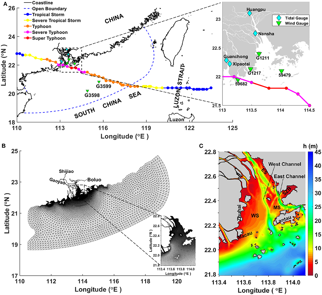
Figure 1. (A) The track and intensity of Typhoon Hato, which crossed the Pearl River Estuary in August 2017. The model domain is bordered by blue dashed lines. The six downward-pointing triangles indicate the locations of wind gauges; the four diamonds represent the locations of tidal gauges. The information on the typhoon track is provided by Zhejiang Water Resources Department (typhoon.zjwater.gov.cn) and that on typhoon intensity is provided by HongKong Observatory (HKO, 2017). (B) The unstructured model grid, which includes 97,602 triangular elements and 56,993 nodes in total; the names of three hydrological stations located at the model's river boundaries are also indicated. (C) Zoomed-in bathymetry around the PRE and its adjacent shelf waters. WS, West Shoal; MS, Middle Shoal; ES, East Shoal; SZB, Shenzhen Bay.

The model was driven by tidal forcing from the OB and atmospheric forcing (i.e., wind stress and sea level pressure, SLP) at the sea surface. Eight tidal constituents (i.e., M₂, S₂, N₂, K₂, K₁, O₁, P₁, Q₁) from the TPXO database (Egbert and Erofeeva, 2002) were used to generate tidal water level time series to drive the model at the open boundary. The atmospheric forcing consisted of hourly 10-m wind speed and SLP with a horizontal resolution of 0.2° (latitude/longitude), which were obtained from the National Centers for Environmental Prediction (NCEP) Climate Forecast System Reanalysis (CFSR) dataset. In order to better describe the typhoon-associated wind field and SLP, blended atmospheric forcing was used in this study by inserting an idealized wind field and SLP for a tropical cyclone, which was calculated by the Holland parametric tropical cyclone model (Holland, 1980), into the original large-scale CFSR atmospheric data (see details in section 7). In addition, high temporal resolution (hourly) observed river discharge from three upstream hydrological stations (i.e., Gaoyao, Shijiao, and Boluo) were used to represent the freshwater inputs from the West River, the North River, and the East River, respectively.

Three sets of numerical experiments were conducted to assess the model performance and to analyze the mechanism of tide-surge interaction:

(a) Full run (Run-Full): The model was driven by both the tidal forcing at the OB and the blended atmospheric forcing. The resultant water level from this model run is the storm tide (ζ_ST).

(b) Storm-only run (Run-SO): Only the blended atmospheric forcing was used to drive the model, while the tidal forcing was turned off. The resultant water level from this model run is called pure storm surge (ζ_SO).

(c) Tide-only run (Run-TO): Only the tidal forcing was included. The resultant water level is the pure astronomical tide level (ζ_TO).

All of the above experiments started from August 1, 2017, and spun up from rest (i.e., zero velocity and undisturbed water level) for the first 4 days; the simulations were then conducted continuously through the whole of August 2017. The split-mode time-stepping method is used in this model, with a 6-s internal time step and a 1-s external time step.

3. Model Evaluation and Validation

3.1. Wind Speed Evaluation

As shown in Figure 1, Hato formed as a tropical depression over the sea northeast of Luzon Island on August 19, 2017, and intensified to a tropical storm over the same waters on August 20. It moved westwards across the Luzon Strait, and intensified to typhoon strength over the northeastern part of the South China Sea on August 22. After that, Hato moved west-northwest toward the coast of China, where it intensified further and became a super typhoon in the early morning of August 23 over the sea south of Hong Kong, reaching its peak intensity with an estimated sustained wind speed of 185 km/h near its center. After making landfall at Zhuhai with severe typhoon intensity, Hato gradually degenerated into a low-pressure system on August 24. Based on the above information, a reconstructed blended wind field for Typhoon Hato was created by using the Holland parametric model (see details in the Appendix). Compared with the original CFSR wind, the blended wind field shows a much larger wind speed near the typhoon center and a more asymmetric vortex structure, which has larger wind speeds on the right-hand side of the typhoon track due to the typhoon translation motion (Figure 2). Especially at 03:00 GMT on 23rd August, when Hato intensified to a super typhoon, the blended data (Figure 2h) clearly reproduced the much stronger typhoon intensity; by contrast, no obvious vortex structure of the typhoon was found in the original CFSR data (Figure 2d). Moreover, the locations of the typhoon center in the blended data are consistent with, while those in the CFSR data deviate more or less from (e.g., Figures 2a,b), those taken from the best track data.

FIGURE 2

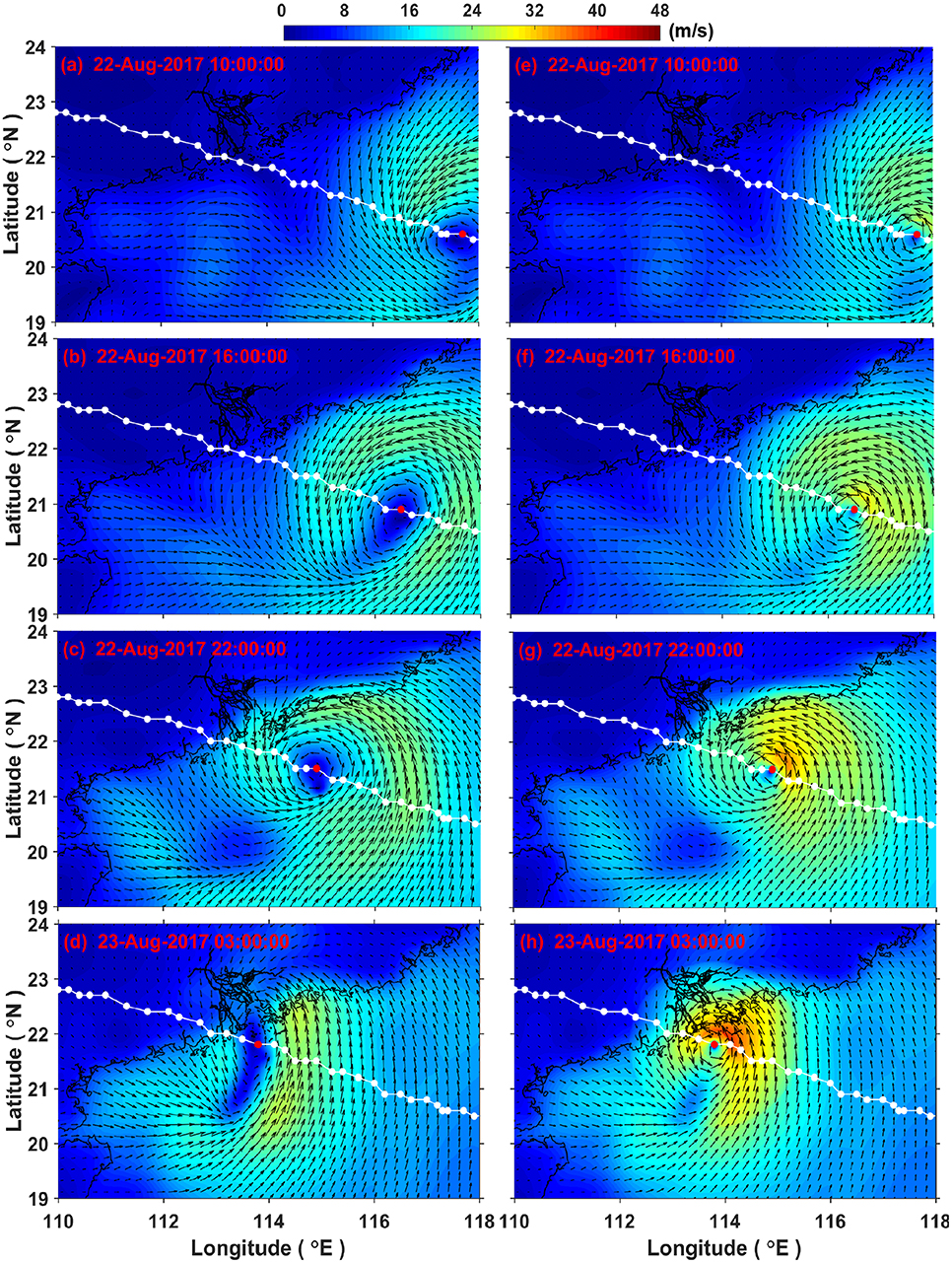
Figure 2. Wind fields from the CFSR dataset (a–d), CFSR, and Holland model blended data (e–h) from 10 GMT on August 22 to 03 GMT on August 23, 2017, when Typhoon Hato moved over the northeastern part of the South China Sea. The white (red) solid circles represent the non-current (current) position of the hourly typhoon center provided by Zhejiang Water Resources Department (typhoon.zjwater.gov.cn ).

In order to qualitatively evaluate both the CFSR and the blended winds, the observed wind speeds from six representative wind gauge stations are used in this study, including stations 59,682 and G3599, which are located near Hato's track center, and G3598, which is relatively far away, and another two locations (i.e., G1217 and 59,479), which are near the entrance of the PRE but also not far from the tropical cyclone track, and an extra one (i.e., G1211), which is located inside the PRE.

The observed and reconstructed wind speeds at the above six stations are compared in Figure 3, in which a common feature of two distinct peaks is observed in the last 10 days of August. The first peak on August 23 results from Typhoon Hato, while the other one is due to another typhoon, Pakhar. In this research, only Hato is analyzed in detail, and thus the blended wind field is only created during its passage (i.e., August 21–24), while for the rest of the time, the blended wind field is identical to the CFSR dataset. When comparing with the observations, it can be seen that the wind speeds based on CFSR are very close to the measurements when Hato's effects are minimal, e.g., between August 15 and August 21, when the typhoon is absent at all stations, and throughout the whole period at G3598, which is far away from the typhoon center. However, the CFSR data severely underestimates the wind speed during the passage of both Typhoon Hato and Typhoon Pakhar. In contrast, the blended approach reproduces both Typhoon Hato's peak wind magnitude and timing well on the whole, although some discrepancies are still observed (e.g., G1211) due to the fact that the parametric tropical cyclone model does not account for the structural changes and wind reduction caused by local land topography. These comparative results suggest that a blended approach is able to achieve a reasonably good estimation of the peak wind stresses under a typhoon condition, while the CFSR data can only be reasonably used with minimal typhoon impacts.

FIGURE 3

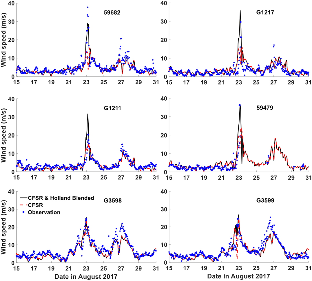
Figure 3. Comparisons of wind speed from CFSR and Holland model blended data (black line), CFSR dataset (red line), and observations (blue dots).

3.2. Water Level Validation

The root-mean-square error (RMSE), correlation coefficient (R), and model skill (Skill) metrics were used to validate the computed water level. The RMSE indicates the average deviation of the model results from the observations and is defined as

$\begin{array}{ll}RMSE=\sqrt{\frac{1}{N}{\displaystyle \sum _{n=1}^N}{(M_n-C_n)}^2}& (10)\end{array}$

where M_n and C_n are the measurements and model computed results, respectively, at N discrete points. CCF and Skill evaluate the coherence between the model results and observations; a CCF or Skill value of 1 indicates a perfect agreement between the model results and measurements, whereas a value of 0 indicates complete disagreement. The CCF is given by

$\begin{array}{ll}CCF=\frac{\frac{1}{N}{\displaystyle \sum _{n=1}^N}(M_n-\overline{M_n})(C_n-\overline{C_n})}{{\sigma }_C{\sigma }_M}& (11)\end{array}$

where σ_C and σ_M are the standard deviations of the model results and measurements, respectively; the overbar represents the mean value. Following Willmott (1981), the Skill formulation is:

$\begin{array}{ll}Skill=1-\frac{{\displaystyle \sum _{n=1}^N}|M_n-C_n{|}^2}{{\displaystyle \sum _{n=1}^N}\left(|M_n-\overline{M_n}{|}^2+|C_n-\overline{M_n}{|}^2\right)}& (12)\end{array}$

The computed astronomical tide was first evaluated at four hydrological stations, Guanchong, Xipaotai, Huangpu, and Nansha, over August 5–31, 2017 (Figure 4). As shown in Table 1, the model predictions follow the reconstructed astronomical tides very well: the RMSE values at all four stations are <0.17 m, and the correlation coefficient (CCF) and model skill (Skill) are generally above 0.96. The model-predicted storm tides at the above four stations were further compared with the total water level observations, as shown in Figure 5. At all of the above four stations, the observed storm tide reaches its maximum (above 2 m) on the morning of August 23, shortly after Typhoon Hato makes landfall. Among these four stations, the recorded storm tide shows a pattern of reaching a single maximum at Huangpu and Nansha, with peak water levels of 2.92 and 3.3 m, respectively. At the other two stations (i.e., Guanchong and Xipaotai), it is interesting to observe that the recorded water level shows a double-peak pattern of “abrupt decline and then rapid rise” in a short time period just before reaching the maximum value on the August 23. This is closely related to the positions of these two stations relative to the typhoon center, which determines the local wind direction, and their relative relationship with the local geometry of the coastline. When Hato moves close but has not made landfall, these two stations are located in the right front quadrant of the typhoon, with offshore winds prevailing locally; a negative storm surge is thus produced, making the local water level drop considerably. After Hato makes a landing, the local wind direction becomes onshore in a short time, with the above two stations lying at the right rear of the typhoon center. The local water level thus increases, with a positive storm surge produced. It is the strong local wind that leads to the significant intensity of the local drop and rise of water level, whereas it is the fast translation speed of Hato that results in the sharp change in water levels from a local minimum to the maximum value.

FIGURE 4

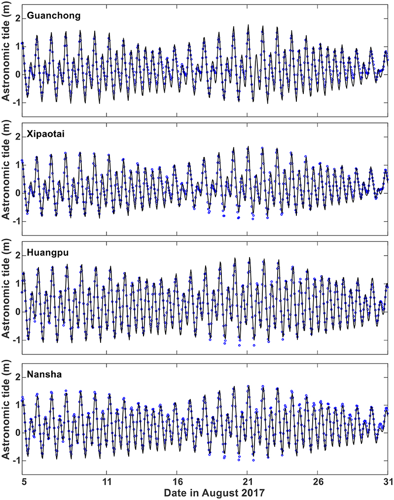
Figure 4. Comparisons of model-predicted (lines) with the reconstructed (circles) astronomical tides over August 5–31, 2017, at the stations of Guanchong, Xipaotai, Huangpu, and Nansha. The reconstructed astronomical tides are calculated from the tidal constituents that were obtained from long-term harmonic analysis of the observed total water levels.

TABLE 1

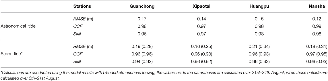
Table 1. Evaluation of model results: the measurements (M_n) used to calculate RMSE, CCF, and Skill for the Astronomical Tide run are the reconstructed astronomical tides from the harmonic analysis results of the observed long-term total water levels, while the measurements used for the validation of the Storm Tide runs are the total water level observations.

FIGURE 5

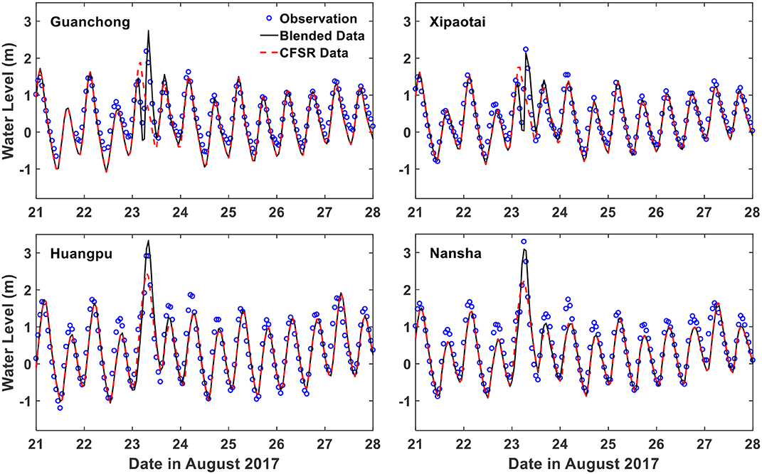
Figure 5. Comparisons of model-predicted (lines) with observed (circles) time series of water level over August 21–28, 2017.

When Hato is far away (i.e., before and after the August 23) from the local stations, the model predicted storm tide from the CFSR wind field agrees well with the observations. However, the CFSR model results severely under-estimate the maximum water levels (e.g., at Nansha station) when Hato moves close; in the meantime, it totally misses the “double-peak” pattern of water level observed at Guanchong and Xipaotai. By contrast, the model-calculated water levels from the blended data agree well with the observations during the whole passage of Typhoon Hato, with both the storm tide maxima and the above “double-peak” pattern of water level well reproduced. The model discrepancies at the time when peak storm tides occur are reduced from 1.37, 1.32, 0.46, and 1.06 m when the original CFSR data is used to 0.42, 0.08, 0.18, and 0.20 m when the blended data is used at the stations of Guanchong, Xipaotai, Huangpu, and Nansha, respectively. Therefore, significant improvements in the model-predicted water levels were obtained in this study by using the blended data shown in the Appendix. Table 1 also shows that the CCF (Skill) at all four stations is above 0.96 (0.94), indicating an overall good agreement of the model-predicted storm tide with the observations over the whole simulation period. However, when we zoom in on the validation period for August 21–24, the CCF (Skill) reduces slightly, while the RMSE increases by more than 9 cm at all four stations. This is largely due to some physical processes being missing in the present model simulations, e.g., wave-induced setup and non-hydrostatic pressure gradients (Zhang et al., 2017).

4. Tide-Surge Interaction and Its Impact

Figure 6 shows the time series of the model-predicted storm tide levels (ζ_ST), astronomical tide levels (ζ_TO), and pure surge elevations (ζ_SO) at the above four tide gauges; they are water level results from the standard experiments Run-Full, Run-TO, and Run-SO, respectively. In addition, two residual water elevations, ζ_PS and ζ_TSI, are also included in Figure 6. The residual water elevation ζ_PS is calculated by subtracting ζ_TO from ζ_ST and is known as the practical storm surge, as defined in most operational storm-surge monitoring systems (Horsburgh and Wilson, 2007; Zhang et al., 2010); while ζ_TSI = ζ_ST − ζ_TO − ζ_SO is the residual elevation due to the tide-surge interaction. The model results show that the magnitudes of ζ_PS near the landfall of Hato are 2–3 m at the four tide gauges and are much larger than their neighboring astronomical tidal high levels. These high water elevations overtopped the coastal sea walls, bringing a large amount of flooding to the coastal areas of the PRE (Li et al., 2018).

FIGURE 6

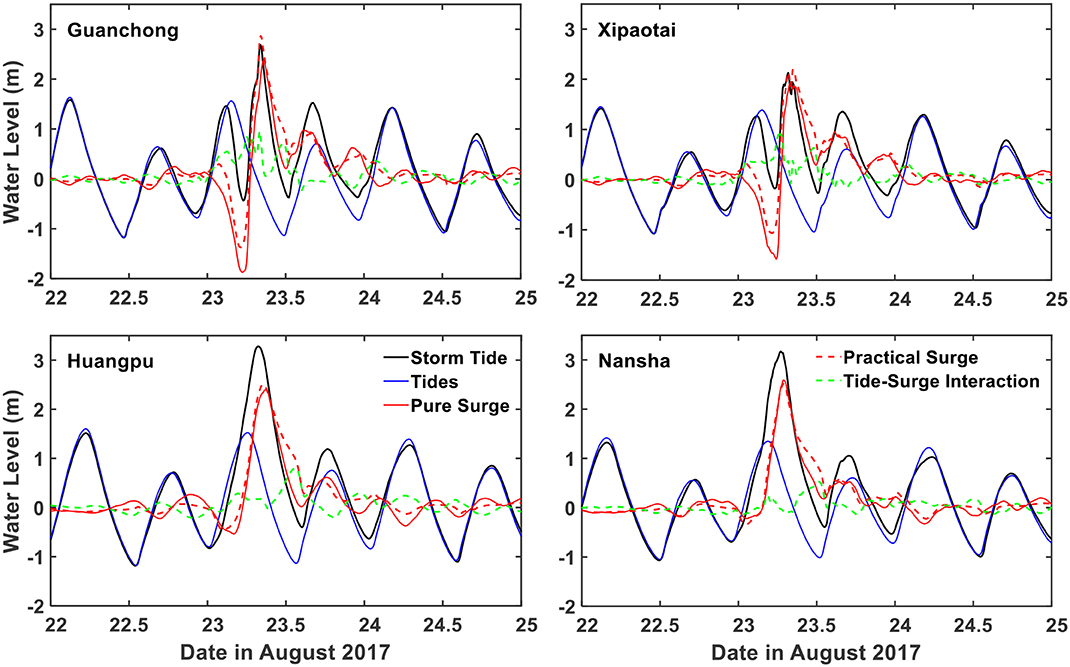
Figure 6. Time series of storm tides (ζ_ST), pure astronomical tides (ζ_TO), pure storm surges (ζ_SO), practical storm surges (ζ_PS), and residual elevations due to the tide-surge interaction (ζ_TSI) over August 22–25, 2017, at Guanchong, Xipaotai, Huangpu, and Nansha stations.

Without tide-surge interaction, the practical storm surge ζ_PS will be equal to the pure storm surge ζ_SO. However, this is generally not true, as shown in Figure 6: the ζ_PS is not equal to ζ_SO during most of the time period at all four stations. The comparison of ζ_PS and ζ_SO shows a general feature, in that the magnitudes of ζ_PS are greater near low tide but smaller near high tide than ζ_SO, especially in the first tidal cycle on August 23, when the storm surge maxima occur. Similar results have also been reported in many previous studies (e.g., Horsburgh and Wilson, 2007; Rego and Li, 2010; Zhang et al., 2010, 2017), reflecting the effects of tidal modulation on surge generation, which can be explained by an idealized expression for the equilibrium between sea surface slope and a constant wind stress term (Pugh, 1996) as follows:

$\begin{array}{ll}\frac{\partial \zeta }{\partial x}=\frac{C_{ds}{U}_w^2}{gD}& (13)\end{array}$

Although such an equilibrium is rarely established in the real world because the wind field changes frequently, Equation (13) illustrates the fundamental point that the wind stress is more effective in producing surges in the shallower waters, e.g., during tidal low waters. In addition to the change of magnitude, the phase of the surge can also be altered by the tide-surge interaction (tidal modulation). Previous studies (e.g., Horsburgh and Wilson, 2007; Wolf, 2009; Rego and Li, 2010), have pointed out that a reduced water depth will result in reduced phase speed both directly and indirectly due to the effects of bottom friction, as it is inversely proportional to the water depth, whereas the enhanced water depth will increase the phase speed. Consistent with the above physics, the peaks of the predicted ζ_PS shown in Figure 6 arrive a bit earlier than those of ζ_SO.

The impact of tidal modulation (tide-surge interaction) on the storm surge and total water levels in the whole PRE can be examined in detail by reference to Figure 7, in which the distribution of the differences between the maxima of ζ_PS and ζ_SO (i.e., ${\zeta }_{PS}^{max}-{\zeta }_{SO}^{max}$; Figure 7A) and the differences between the maxima of ζ_ST and ζ_SO + ζ_TO (i.e., ${\zeta }_{ST}^{max}-{\left[{\zeta }_{SO}+{\zeta }_{TO}\right]}^{max}={\left[{\zeta }_{PS}+{\zeta }_{TO}\right]}^{max}-{\left[{\zeta }_{SO}+{\zeta }_{TO}\right]}^{max}$; Figure 7B) are presented. In these figures, two notable features can be observed: firstly, the spatial distributions of both differences defined above show considerable variations in the PRE, indicating that the effect of tide-surge interaction is highly localized and spatially varying; secondly, both of the tidally modulated peak water elevations (i.e., ζ_PS, ζ_ST) have higher magnitudes near the east coast but smaller magnitudes close to the west coast of the PRE than those predicted without the effects of tide (i.e., ζ_SO, [ζ_SO + ζ_TO]), which confirms previous studies (e.g., Brown et al., 2010; Quinn et al., 2012) in showing that tide-surge interaction can either enhance or reduce the peak surge elevations. More detailed examinations of the magnitudes show that the peak water elevations at Shenzhen Bay are significantly raised by 0.1–0.5 m due to tide-surge interaction, whereas, in the coastal area of Zhuhai and Macau, the peak water elevations are reduced by 0.2–0.4 m. From a surge-protection point of view, the increase in the water level shown in Figures 7A,B is of more practical significance, as an underestimation of the peak water elevations, e.g., near the east PRE coast in this study when the effect of tide-surge interaction is not taken into account, could lead to huge economic loss and high fatalities.

FIGURE 7

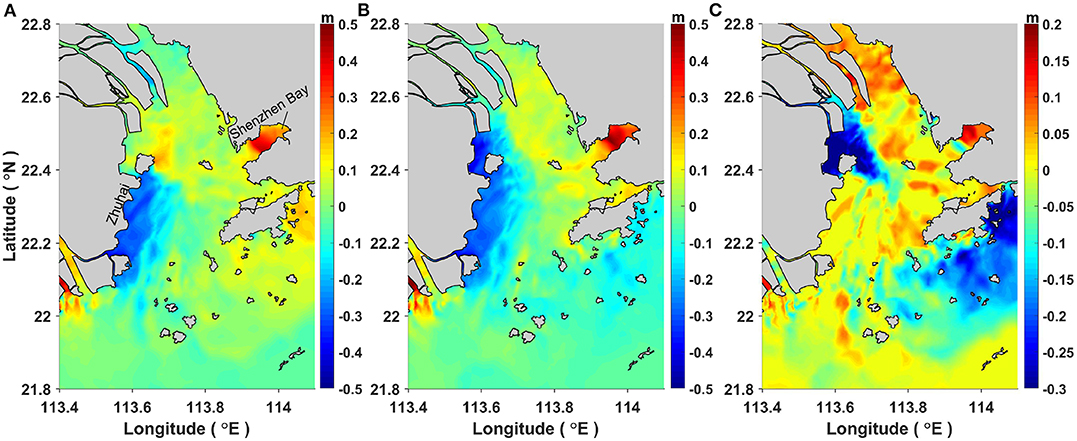
Figure 7. Spatial distributions of (A) the differences between the maxima of ζ_PS and ζ_SO (i.e., ${\zeta }_{PS}^{max}-{\zeta }_{SO}^{max}$), (B) the differences between the maxima of ζ_ST and ζ_SO + ζ_TO (i.e., ${\zeta }_{ST}^{max}-{\left[{\zeta }_{SO}+{\zeta }_{TO}\right]}^{max}={\left[{\zeta }_{PS}+{\zeta }_{TO}\right]}^{max}-{\left[{\zeta }_{SO}+{\zeta }_{TO}\right]}^{max}$), and (C) the differences between (A,B) $(i.e.,\left\{{\zeta }_{ST}^{max}-{\left[{\zeta }_{SO}+{\zeta }_{TO}\right]}^{max}\right\}-\left\{{\zeta }_{PS}^{max}-{\zeta }_{SO}^{max}\right\})$, during the passage of Typhoon Hato.

The differences in the maxima of the practical storm surge ζ_PS and the pure storm surge ζ_SO (i.e., ${\zeta }_{PS}^{max}-{\zeta }_{SO}^{max}$) in Figure 7A represent the tide-surge interaction-induced changes in the magnitude of the storm surge. By contrast, the differences between the maximum elevations of ζ_ST and ζ_SO + ζ_TO (i.e., ${\zeta }_{ST}^{max}-{\left[{\zeta }_{SO}+{\zeta }_{TO}\right]}^{max}={\left[{\zeta }_{PS}+{\zeta }_{TO}\right]}^{max}-{\left[{\zeta }_{SO}+{\zeta }_{TO}\right]}^{max}$) in Figure 7B include the effects from the tide-surge interaction on both the magnitudes and phases of the storm surge. The fact that the tide-surge interaction not only influences the surge level but also the peak timing of the storm surge is clearly reflected in the contrast between Figures 7A,B, which is also detailed in Figure 7C. A close examination of Figure 7C suggests that the phase alteration mainly increases (i.e., positive magnitudes) the peak total water elevations (i.e., the storm tide elevation ζ_ST) in the majority of the PRE. One of the most notable areas is near the top of Shenzhen Bay, where a maximum magnitude of 0.18 m is found, which is largely caused by the phase alteration due to the nonlinear shallow water effects (see details in section 5.2). The above analysis indicates that both the tidally modulated surge generation and phase alteration contribute considerably to the peak overall water elevations; a linear superposition of the atmospheric-only forced pure storm surge (ζ_SO) with the astronomical tide (ζ_TO) can deviate from the real conditions significantly, as shown in Figure 7, and thus the effects of non-linear tide-surge interactions are vitally important.

As noted in previous studies (Horsburgh and Wilson, 2007; Wolf, 2009; Rego and Li, 2010), the modulation of surge generation and propagation shown above represents the effect of tide on the surge, while the effect of surge on the tide is largely presented as a phase shift of the tidal signal. These mutual influences between the tide and surge contribute to the total effects of tide-surge interaction. Since the residual water elevation ζ_TSI, calculated as ζ_ST−ζ_TO−ζ_SO, is the result of tide-surge interaction, it has been taken as a direct measure of the interaction intensity in previous studies (e.g., Bernier and Thompson, 2007; Rego and Li, 2010; Zhang et al., 2010, 2017). Figure 6 shows that ζ_TSI is negligible before and after the passage of Typhoon Hato and that it increases greatly in magnitude as the storm surge develops at all stations. Notable oscillations with a near-tidal period are found in ζ_TSI, which is very likely due to the effect of tidal modulation. To quantify the absolute intensity of tide-surge interaction, some studies (e.g. Horsburgh and Wilson, 2007; Rego and Li, 2010; Zhang et al., 2017) have used various different indicators, including the maximum positive (MAX) or minimum negative (MIN) magnitude of ζ_TSI, whereas some others (e.g., Bernier and Thompson, 2007; Rego and Li, 2010; Zhang et al., 2010) have used the root-mean-square value (RMS) of ζ_TSI¹, as the representative variable. Evidently, RMS(ζ_TSI) represents the average intensity of tide-surge interaction, while MAX(ζ_TSI) and MIN(ζ_TSI) are more concerned with the maximum intensity that occurs during an entire typhoon event. For Typhoon Hato, the spatial distributions of MAX(ζ_TSI) and RMS(ζ_TSI) in the PRE are shown in Figures 8A,B, respectively. Both of these figures demonstrate the feature that the intensity of tide-surge interaction is strongest in the top of the PRE and Shenzhen Bay and gradually decreases from the estuary/bay head to the estuary/bay entrance, as the bell-shaped geometry can amplify the impact of tide-surge interaction. MAX(ζ_TSI) is about 0.18–0.6 m in the PRE, whereas the magnitude of RMS(ζ_TSI) is much smaller (0.07–0.25 m). The contrast between MAX(ζ_TSI) and RMS(ζ_TSI) indicates that the effect of tide-surge interaction varies strongly over time, which coincides with the distribution pattern of ζ_TSI as shown in Figure 6, so that the majority of the energy of the tide-surge interaction is concentrated near the time when the largest storm surge occurs. Besides MAX(ζ_TSI) and RMS(ζ_TSI), a new indicator I_r is also plotted in Figure 8C. It is defined as the ratio of RMS(ζ_TSI) to the square root of the product of RMS(ζ_SO) and RMS(ζ_TO), i.e., $I_r=RMS({\zeta }_{TSI})/\sqrt{RMS({\zeta }_{SO})*RMS({\zeta }_{TO})}$, and is used to reflect the total relative intensity of tide-surge interaction to pure storm surge and pure astronomical tide, similar to that in Zhang et al. (2010). A similar feature is found in Figure 8C as is shown in Figures 8A,B. As the intensity of tide-surge interaction increases in proportion to both surge height and tidal range (Horsburgh and Wilson, 2007), I_r is considered to be more appropriate to quantify the relative importance of different physical processes in studying the mechanisms of tide-surge interaction (see details in section 5).

FIGURE 8

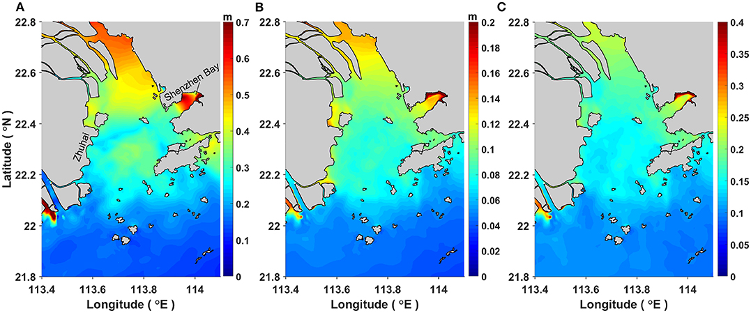
Figure 8. Spatial distributions of (A) the maximum positive magnitude of ζ_TSI, i.e., MAX(ζ_TSI), (B) the root-mean-square of ζ_TSI, i.e., RMS(ζ_TSI), and (C) the ratio I_r, which is defined as $I_r=RMS({\zeta }_{TSI})/\sqrt{RMS({\zeta }_{SO})*RMS({\zeta }_{TO})}$, in the PRE during the passage of Typhoon Hato.

5. Mechanism Analysis of Tide-Surge Interaction

5.1. The “Subtraction” Approach

To assess the contribution of each nonlinear physical process to the tide-surge interaction, previous studies (Bernier and Thompson, 2007; Zhang et al., 2010, 2017) conducted numerical experiments using a reduced model approach in which the non-linear terms associated with each physical process were eliminated or linearized: (1) to quantify the nonlinear advective effect (Exp-LAdv), the advective terms were removed from Equations (1) and (2); (2) to quantify the nonlinear bottom friction effect (Exp-LBot), the quadratic form of bottom friction was linearized by using (τ_bx, τ_by) = ρ₀C_db (u, v); (3) to quantify the shallow water effect (Exp-LSW), the total water depth D = h + ζ in the governing equations was replaced by h. Therefore, this approach can be regarded as a “subtraction approach,” as it is based on a standard model that includes all three processes and assesses the changes to the interaction intensity after one of the processes is removed. Various aspects of this approach are also briefly summarized in Table 2. Following the same procedure as in the standard experiment (Exp-SD, i.e., the experiment conducted using the complete model including all three processes; section 4), three model runs (i.e., Run-Full, Run-TO, and Run-SO) were conducted in each reduced-model experiment, from which the corresponding residual elevations due to tide-surge interaction (i.e., ${\zeta }_{TSI}^{LAdv}$, ${\zeta }_{TSI}^{LBot}$, and ${\zeta }_{TSI}^{LSW}$) are calculated. The contribution from each process is then assessed by quantifying the extent to which the intensity of tide-surge interaction is reduced. For this purpose, Zhang et al. (2010) calculated a reduction ratio of RMS(ζ_TSI), i.e., I_p, whereas Zhang et al. (2017) closely compared the MAX(ζ_TSI) value calculated by the reduced experiments with that obtained from the standard experiment. I_p is defined as follows (Zhang et al., 2010):

$\begin{array}{ll}{I}_p=\frac{RMS({\zeta }_{TSI}^{SD})-RMS({\zeta }_{TSI}^{*})}{RMS({\zeta }_{TSI}^{SD})}\times 100\%& (14)\end{array}$

where $RMS({\zeta }_{TSI}^{SD})$ and $RMS({\zeta }_{TSI}^{*})$ are root-mean-square of ζ_TSI obtained from the standard experiment and reduced experiments, respectively, and * represents either LAdv, LBot, or LSW.

TABLE 2

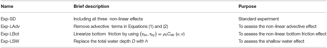
Table 2. The “subtraction” numerical approach used to study the mechanisms of tide-surge interaction.

Although the contribution from each process can be discerned on close comparisons of the interaction intensity between the results from a reduced model and the standard model as in Zhang et al. (2017), it is best visualized through detailed analysis of the differences obtained by subtracting the interaction intensity of a reduced model from that of the standard model. The reduction ratio R_o, based on a generalized form of I_p in Equation (14), is employed to quantify the reduction of tide-surge interaction intensity as follows:

$\begin{array}{ll}{R}_o=\frac{P^{SD}-P^{*}}{P^{SD}}\times 100\%& (15)\end{array}$

where P is a general indicator used to represent the intensity of tide-surge interaction, e.g., MAX(ζ_TSI), RMS(ζ_TSI), or I_r; SD represents the standard experiment, and * represents either LAdv, LBot, or LSW.

The calculated R_o over the PRE is shown in Figures 9A–I for the reduced experiments Exp-LAdv, Exp-LBot, and Exp-LSW, respectively. All three indicators, MAX(ζ_TSI), RMS(ζ_TSI), and I_r, are used to represent the intensity of tide-surge interaction and to calculate the corresponding R_o. In the present approach, the contribution from each physical process is expected to lead to a nonnegative reduction ratio (R_o), with its magnitude indicating the strength of contribution. However, negative values of R_o are found in all three reduced experiments based on all three intensity indicators (RMS, I_r, and MAX) in Figures 9A–I. This common feature suggests that it is more likely that the “subtraction” approach is the reason for the negative reduction ratio rather than that inappropriate indicators are being used. Similar results were also observed in several previous studies (e.g., Tang et al., 1996; Zhang et al., 2017). As explained in Zhang et al. (2017), this phenomenon is due to the “rebalance” effect: in each of the three reduced experiments, when one physical process is removed, the remaining two processes will increase their strength to rebalance the governing equations; a larger intensity of tide-surge interaction induced by these two processes is thus obtained, which leads to a negative R_o. Furthermore, the change in the strengths of the remaining two processes (e.g., the nonlinear bottom friction effect and shallow water effect) indicates that the tide-surge interaction intensities induced by these two processes from a reduced model (i.e., P^*) are different from those included in the standard model (i.e., those included in P^SD). Even if the value of P^SD−P^* is positive, it may not be correct for the intensity induced by the first process (e.g., the nonlinear advective effect). This means that in addition to negative R_o values being produced, positive R_o values can be influenced by the “rebalance” effect. The R_o shown in Figure 9, whether positive or negative, thus cannot correctly represent the contribution from one non-linear process properly. An “addition” approach is therefore developed in the next section in order to improve the analysis.

FIGURE 9

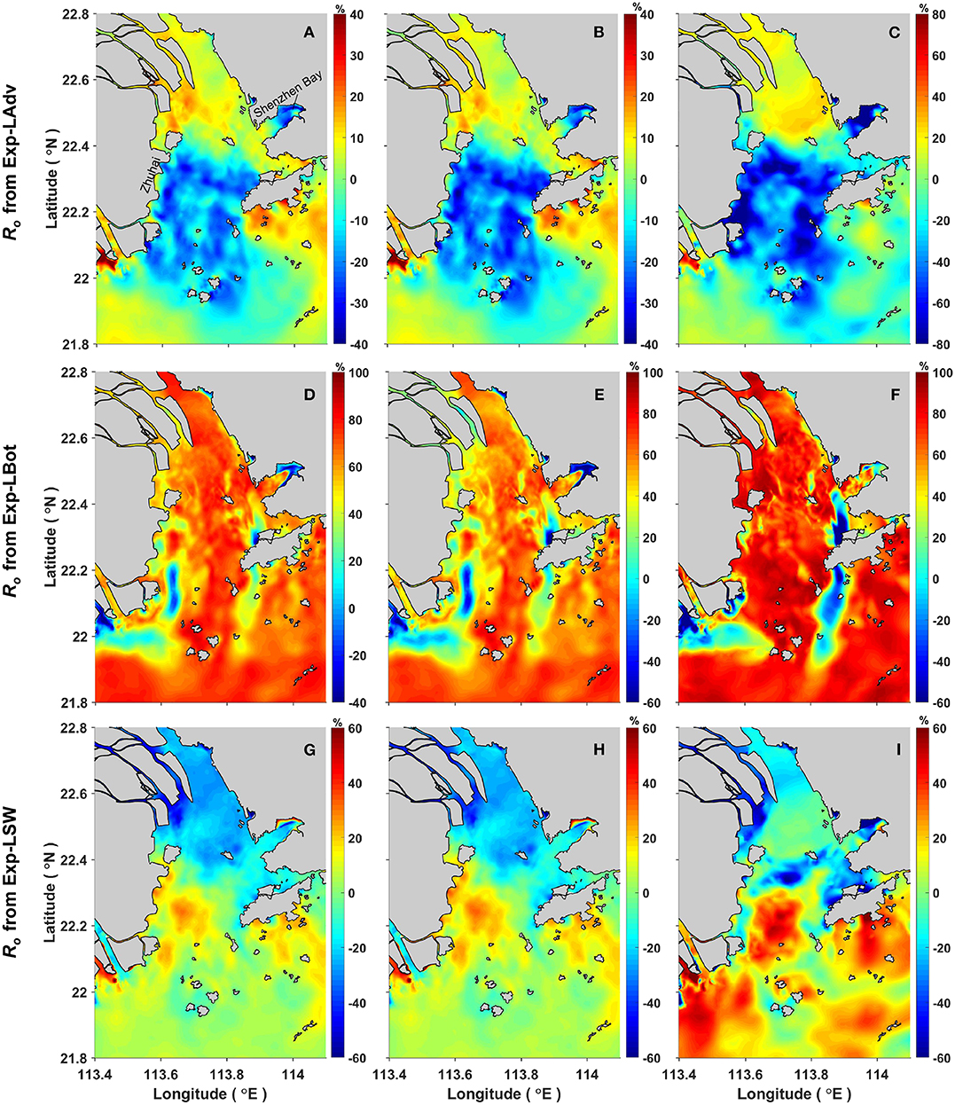
Figure 9. Spatial distributions of the reduction ratio R_o in the PRE. (A–C) Show the R_o values calculated by using RMS(ζ_TSI), I_r, and MAX(ζ_TSI), respectively, from the reduced experiment Exp-LAdv; (D–F) show the R_o values calculated by using RMS(ζ_TSI), I_r, and MAX(ζ_TSI), respectively, from the reduced experiment Exp-LBot; (G–I) show the R_o values calculated by using RMS(ζ_TSI), I_r, and MAX(ζ_TSI), respectively, from the reduced experiment Exp-LSW.

5.2. The “Addition” Approach

Due to the defects found in the above “subtraction” numerical approach, a new method is proposed in this section in order to clearly separate the contributions of the three physical processes and quantify their relative contributions to the tide-surge interaction. As introduced in section 5.1, the “subtraction” approach quantifies the contribution of one specific process to the tide-surge interaction by removing/linearizing its corresponding momentum terms from the standard model. After this operation, each reduced model still contains two of three non-linear effects. In contrast, the present new approach takes an “addition” approach (Table 3): (a) firstly, a base experiment (Exp-None) was conducted using a reduced model with all three non-linear effects removed; (b) three experiments (Exp-AAdv, Exp-ABot, Exp-ASW) were then carried out, each only taking one non-linear effect into account; (c) following the same method as in the standard experiment and the “subtraction” approach, the astronomical tide (ζ_TO), surge (ζ_SO), and tide-surge interaction residual (ζ_TSI) values corresponding to the above four experiments were obtained.

TABLE 3

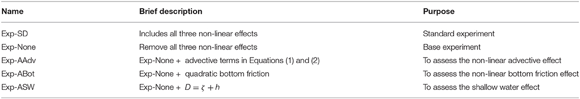
Table 3. The new numerical approach used to study the mechanisms of tide-surge interaction.

To assess the quantification of the contribution from each physical process to the tide-surge interaction, a new ratio R_n is defined as follows:

$\begin{array}{ll}{R}_n=\frac{P^{**}-P^{None}}{P^{SD}}\times 100\%& (16)\end{array}$

where P is the general indicator used to represent the intensity of tide-surge interaction as used in Equation (15), SD represents the standard experiment, and ** represent either AAdv, ABot, or ASW. It should be noted that although the ζ_TSI obtained from the base experiment (Exp-None) should theoretically be zero as all three nonlinear physical processes are removed, it, in fact, has a magnitude of O(mm) due to the existence of numerical errors.

As only one process is included in a specific reduced model, the interaction intensity induced by this process will not be affected by the other two processes. Figure 10 shows the R_n values calculated from the reduced experiments Exp-AAdv (Figures 10A–C), Exp-ABot (Figures 10D–F), and Exp-ASW (Figures 10G–I), respectively, by using all of the three representative intensity indicators. As expected, positive R_n values were obtained in all cases. For the same reduced experiment, the spatial distribution pattern of R_n calculated from RMS(ζ_TSI) is very close to that calculated from I_r, indicating that these two indicators of interaction intensity, RMS(ζ_TSI) and I_r, provide similar quantification of the relative contributions from the physical processes. However, the spatial distribution of R_n values calculated from RMS(ζ_TSI) (or I_r) and that from MAX(ζ_TSI) are very different. This can be explained as follows: both RMS(ζ_TSI) and I_r represent the average intensity, whereas MAX(ζ_TSI) represents the maximum intensity of tide-surge interaction that occurs during an entire typhoon event. The magnitudes of R_n calculated from RMS(ζ_TSI) and I_r also differ from each other, indicating that the pure storm surge levels (ζ_SO) and pure astronomical tide elevations (ζ_TO) in the reduced experiments are not the same as those in the standard experiment. As the tide-surge interaction increases in direct proportion to both surge height and tidal range, a larger RMS(ζ_TSI) or MAX(ζ_TSI) in the reduced experiment may be due to the larger surge height and/or the larger tidal range but not necessarily due to the corresponding nonlinear physical processes themselves. Therefore, it is not appropriate to use RMS(ζ_TSI) or MAX(ζ_TSI) to represent the contributions from the three physical processes to the tide-surge interaction. In contrast, the ratio I_r, as shown in Equation (16), reflects the total relative intensity of tide-surge interaction to the pure storm surge and pure astronomical tide, thus eliminating the influences of the changes in surge height and tidal range on the interaction intensity. It is therefore more reasonable to use I_r rather than RMS(ζ_TSI) or MAX(ζ_TSI) to quantify the relative contribution from the three physical processes.

FIGURE 10

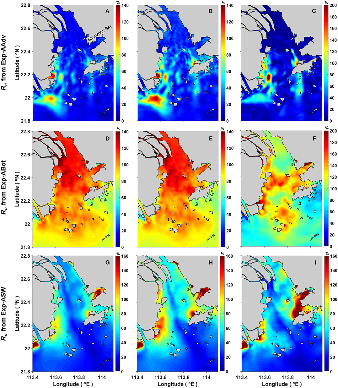
Figure 10. Similar as Figure 9 but for R_n calculated by the “addition” numerical approach as described in section 5.2. (A–C) Show R_n values calculated by using RMS(ζ_TSI), I_r, and MAX(ζ_TSI), respectively, from the reduced experiment Exp-AAdv; (D–F) show the R_n values calculated by using RMS(ζ_TSI), I_r, and MAX(ζ_TSI), respectively, from the reduced experiment Exp-ABot; (G–I) show the R_n values calculated by using RMS(ζ_TSI), I_r, and MAX(ζ_TSI), respectively, from the reduced experiment Exp-ASW.

The results in Figures 10D–F also show a common feature that the calculated R_n in some areas of the PRE is larger than 100%, indicating that the intensity of tide-surge interaction due to one of those processes alone is larger than that obtained from the standard model, in which all three are included. This is a very interesting result, which suggests that certain interactions must have taken place between those three processes and that, for some areas in the PRE, the result of this interaction is to reduce the magnitude of the contribution from the individual processes. In addition, this phenomenon may also be one of the reasons that the “rebalance effect” described in section 5.1 occurs: when one of the three physical processes is removed from the standard model, the remaining processes in the reduced model still interact with each other in a somewhat different way; the “rebalance effect” thus occurs. This finding therefore further indicates that the “addition” approach is a better choice to avoid complication in the quantification of the tide-surge interaction.

From Figure 10, the relative contributions from the three processes to the tide-surge interaction can be directly compared based on the magnitude of R_n obtained from the three reduced experiments in specific regions in the PRE. For instance, the results demonstrate that the quadratic bottom friction is most significant in the majority of the PRE, whereas, at the top of Shenzhen Bay, the shallow water effect is more significant due to the limited water depth over the tidal flat. To get a clear overview of the overall contribution from the three processes in the whole PRE, the R_n values obtained from the three reduced models are firstly compared with each other and then sorted at every model grid according to their magnitudes. Subsequently, based on the RMS(ζ_TSI) indicator, the process with the largest R_n value at each grid node is plotted using its specific color code in Figure 11A. Similarly, the process with the second R_n is presented in Figure 11B and with the smallest R_n in Figure 11C. Taking the top of Shenzhen Bay as an example, Figure 11A shows that the most important non-linear process there is the shallow water effect (represented in blue); the second most important nonlinear process, shown in Figure 11B, is the quadratic bottom friction (represented in green); and the third most important nonlinear process, shown in Figure 11C, is the non-linear advective effect (represented in red). In a similar way, the processes with the largest R_n, second R_n, and smallest R_n based on the I_r indicator are shown in Figures 11D–F, and those based on the MAX(ζ_TSI) indicator are shown in Figures 11G–I. The processes with the largest, second, and smallest contribution at any location can thus be directly identified from the corresponding color code. Meanwhile, the area covered by one specific color represents the overall relative importance in the PRE overall. Clearly, no matter which intensity index is used, the results demonstrate a common conclusion that among all the largest-contribution figures (Figures 11A,D,G), the quadratic bottom friction occupies the largest area, which means that the bottom friction contributes the most to the tide-surge interaction. In the second-contribution figures (Figures 11B,E,H), the shallow water effect is clearly the most significant, and hence it contributes to the tide-surge interaction at the second level. Non-linear advection is the third most significant contributor over the majority of the area of the PRE, as shown in Figures 11C,F,I. Similar to those shown in Figure 10, the results obtained from I_r are close to those from RMS(ζ_TSI) but are different from MAX(ζ_TSI) at certain locations. For example, at the top of Shenzhen Bay, Figure 11D demonstrates that the shallow water effect dominates, whereas Figure 11G shows the quadratic bottom friction as more important. Due to its shallow water depth, this area is expected to be more significantly affected by the shallow water effect. Therefore, as demonstrated above, the I_r value expressed in Equation (16) is recommended for use for the quantification of the contributions from any particular process.

FIGURE 11

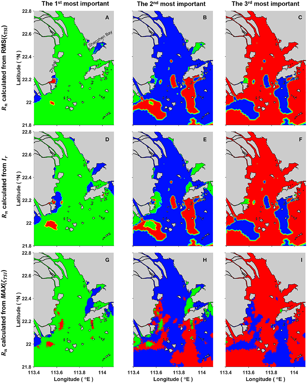
Figure 11. The first (A,D,G), second (B,E,H), and third (C,F,I) most important non-linear effects in the tide-surge interaction in the PRE. Green represents the quadratic bottom friction; blue represents the shallow water effect; and red represents the nonlinear advective effect. (A–C) Use RMS(ζ_TSI) to calculate R_n, (D–F) use I_r to calculate R_n, and (G–I) use MAX(ζ_TSI) to calculate R_n.

6. Summary and Conclusions

In this study, the characteristics and mechanisms of tide-surge interaction in the Pearl River Estuary during Typhoon Hato are studied in detail by using a 3D ocean model (Zheng P. et al., 2017). Along with the use of a blended atmospheric forcing, which merged the Holland parametric model results with the CFSR reanalysis data, the model reproduces the pure astronomical tides and total sea levels reasonably well, especially at Guanchong and Xipaotai, where the distinctive “double-peak” pattern observed in the measured water levels is well-reproduced by the present model.

To study the characteristics of tide-surge interaction in the PRE, three types of model runs were conducted, from which the total water level (storm tide ζ_ST), the pure storm surge (ζ_SO), the pure astronomical tide level (ζ_TO), the practical storm surge (ζ_PS), and the residual elevation due to the tide-surge interaction (ζ_TSI) were obtained. These results show that, due to the tide-surge interaction, the storm surge is clearly modulated by the tide level, e.g., the magnitudes of ζ_PS are greater near low tide but smaller near high tide than ζ_SO. The timing of the surge is also altered due to the tidal modulation effect, and the peaks of the predicted ζ_PS shown in Figure 6 arrive a bit earlier than those of ζ_SO. The horizontal distributions of the differences between ${\zeta }_{PS}^{max}$ and ${\zeta }_{SO}^{max}$ (and the differences between ${\zeta }_{ST}^{max}$ and ${\left[{\zeta }_{SO}+{\zeta }_{TO}\right]}^{max}$) show that the effect of tide-surge interaction can either enhance or reduce the peak surge elevations. In addition, the resultant phase alteration can also affect the peak total water elevation (ζ_ST). A close examination of Figure 7C indicates that the phase alteration significantly increases the peak ζ_ST in the majority of the PRE. One of the most notable areas affected by such a process is near the top of Shenzhen Bay, where a maximum magnitude of 0.18 m is found. Three indicators were used to quantify the absolute intensity of tide-surge interaction, namely the previously used MAX(ζ_TSI) and RMS(ζ_TSI) and a newly proposed I_r, which reflects the total intensity of tide-surge interaction relative to pure storm surge and pure astronomical tide. As I_r eliminates the dependence of the interaction intensity on the magnitude of surge height and tidal range, it is considered more appropriate for use in quantifying the relative importance of different physical processes to tide-surge interaction.

A widely used “subtraction” approach and a newly proposed “addition” approach are adopted to separate the contributions of three non-linear processes to tide-surge interaction and to quantify their relative significance, respectively. In the widely used “subtraction” approach, each of the three processes is removed or linearized from a standard model that includes all processes. The contribution from each specific process to the tide-surge interaction is quantified based on the reduction ratio (R_o) of interaction intensity. However, the results show that the R_o value from the “subtraction” approach is greatly affected by the “rebalance” effect (Figure 9); Thus, it can not correctly represent the significance of its corresponding nonlinear process. An “addition” approach is therefore proposed in which one of the three processes is added onto the baseline simulation without any non-linear effects. A new general ratio R_n is defined to quantify the contribution of each process, the value of which can be calculated from any one of three representative indicators of tide-surge interaction intensity. The comparison of the magnitudes of R_n between those obtained from the three reduced experiments clearly shows that the quadratic bottom friction, shallow water effect, and nonlinear advective effect have the largest, second-largest, and third-largest contributions to the tide-surge interactions in the majority of the PRE, respectively. Among the three indicators that have been used to represent the intensity of tide-surge interaction, I_r is suggested to be more reasonable for use to quantify the relative importance of the three non-linear effects.

Taking Typhoon Hato as a case study, the present research reveals the detailed characteristics of tide-surge interaction in the PRE. The present results are able to provide valuable information for the coastal defense management of different regions inside the PRE, although studies on more typhoon events may be needed. Furthermore, the mechanism of tide-surge interaction is examined by using a newly proposed “addition approach.” This new approach is free of the problems caused by the “rebalance” effect and thus is recommended for use in future similar studies and in other regions of the world.

Data Availability Statement

To enable use of the data from the present study by the readers and to achieve further understanding of tide-surge interaction processes, a database hosted by the University of Liverpool (UK) is available at the website: http://datacat.liverpool.ac.uk/id/eprint/1070.

Author Contributions

PZ took part in all activities in this research, including writing the first draft of the paper, model setup and experimental design, and model results analysis. He also proposed the new addition approach and the use of the I_r indicator to represent the tide-surge interaction after some inspiring discussions with ML. ML modified the first draft of the paper throughout, helped PZ to design the model experiments, and also gave advice in drafting the final paper. CW designed the approach used to reconstruct the Typhoon Hato wind field by merging the CFSR winds and Holland parametric model results. She also provided the observed wind data at six stations and made a preliminary comparison between the reconstructed and observed wind at six stations. JW and XC helped PZ to analyze the model results, they also made some very useful modifications to the draft paper, which greatly improved the readability and completeness of the draft. MD and PY helped PZ to create the model mesh grid and to determine the basic model configuration. JW and ZH are the project co-PIs, they provided critical data and revision advice on the structure of the manuscript. All the authors participated in the revision of the manuscript.

Funding

This research was jointly sponsored by the National Key Research and Development Project (China, 2016YFC1401300), Engineering and Physical Sciences Research Council (United Kingdom, No. EP/R024537/1), National Natural Science Foundation of China (China, No. 51761135022), Dutch Research Council (NWO, the Netherlands, No. ALWSD.2016.026), and Guangdong Provincial Department of Science and Technology (China, 2019ZT08G090).

Conflict of Interest

The authors declare that the research was conducted in the absence of any commercial or financial relationships that could be construed as a potential conflict of interest.

Acknowledgments

Computational support was provided by the Barkla High-Performance Computer at the University of Liverpool and the ARCHER UK National Supercomputing Service (http://www.archer.ac.uk).

Footnotes

1. ^The root-mean-square (RMS) of ζ_TSI is defined as $RMS({\zeta }_{TSI})=\sqrt{{\int }_{\Delta T}{\zeta }_{TS{I}^{dt/\Delta T,}}^2}$, in which ΔT represents the duration of the typhoon event.

References

Bernier, N. B., and Thompson, K. R. (2007). Tide-surge interaction off the east coast of Canada and Northeastern United States. J. Geophys. Res. 112:C06008. doi: 10.1029/2006JC003793

CrossRef Full Text | Google Scholar

Bertin, X., Bruneau, N., Breilh, J.-F., Fortunato, A. B., and Karpytchev, M. (2012). Importance of wave age and resonance in storm surges: the case Xynthia, Bay of Biscay. Ocean Modell. 42, 16–30. doi: 10.1016/j.ocemod.2011.11.001

CrossRef Full Text | Google Scholar

Bobanović, J., Thompson, K. R., Desjardins, S., and Ritchie, H. (2006). Forecasting storm surges along the east coast of Canada and the North-Eastern United States: the storm of 21 January 2000. Atmos. Ocean 44, 151–161. doi: 10.3137/ao.440203

CrossRef Full Text | Google Scholar

Brown, J. M., Souza, A. J., and Wolf, J. (2010). An 11-year validation of wave-surge modelling in the Irish sea, using a nested polcoms-wam modelling system. Ocean Modell. 33, 118–128. doi: 10.1016/j.ocemod.2009.12.006

CrossRef Full Text | Google Scholar

Carr, L. E., and Elsberry, R. L. (1997). Models of tropical cyclone wind distribution and beta-effect propagation for application to tropical cyclone track forecasting. Month. Weath. Rev. 125, 3190–3209. doi: 10.1175/1520-0493(1997)125<3190:MOTCWD>2.0.CO;2

CrossRef Full Text | Google Scholar

Chen, C., Liu, H., and Beardsley, R. C. (2003). An unstructured grid, finite-volume, three-dimensional, primitive equations ocean model: application to coastal ocean and estuaries. J. Atmos. Ocean. Technol. 20, 159–186. doi: 10.1175/1520-0426(2003)020<0159:AUGFVT>2.0.CO;2

CrossRef Full Text | Google Scholar

Doodson, A. T. (1956). Tides and storm surges in a long uniform gulf. Proc. R. Soc. Lond. Ser. A Math. Phys. Sci. 237, 325–343. doi: 10.1098/rspa.1956.0180

CrossRef Full Text | Google Scholar

Egbert, G. D., and Erofeeva, S. Y. (2002). Efficient inverse modeling of barotropic ocean tides. J. Atmos. Ocean. Technol. 19, 183–204. doi: 10.1175/1520-0426(2002)019<0183:EIMOBO>2.0.CO;2

CrossRef Full Text | Google Scholar

Fujita, T. (1952). Pressure distribution within typhoon. Geophys. Mag. 23, 437–451.

Google Scholar

Graber, H. C., Cardone, V. J., Jensen, R. E., Slinn, D. N., Hagen, S. C., Cox, A. T., et al. (2006). Coastal forecasts and storm surge predictions for tropical cyclones: a timely partnership program. Oceanography 19, 609–646. doi: 10.5670/oceanog.2006.96

CrossRef Full Text | Google Scholar

Graham, H., and Nunn, D. (1959). Meteorological Conditions Pertinent to Standard Project Hurricane. Washington, DC: Atlantic and Gulf Coasts of United States; Weather Bureau, US Department of Commerce.

Google Scholar

Harper, B., Hardy, T., Mason, L., Bode, L., Young, I., and Nielsen, P. (2001). Queensland Climate Change and Community Vulnerability to Tropical Cyclones: Ocean Hazards Assessment-Stage 1. Report prepared by Systems Engineering Australia in conjunction with James Cook University Marine Modelling Unit, Queensland Government.

Google Scholar

HKO (2017). Hong Kong Observatory: Tropical Cyclones in 2017

Google Scholar

Holland, G. J. (1980). An analytic model of the wind and pressure profiles in hurricanes. Mon. Weather Rev. 108, 1212–1218. doi: 10.1175/1520-0493(1980)108<1212:AAMOTW>2.0.CO;2

CrossRef Full Text | Google Scholar

Horsburgh, K., and Wilson, C. (2007). Tide-surge interaction and its role in the distribution of surge residuals in the North Sea. J. Geophys. Res. 112:C08003. doi: 10.1029/2006JC004033

CrossRef Full Text | Google Scholar

Jakobsen, F., and Madsen, H. (2004). Comparison and further development of parametric tropical cyclone models for storm surge modelling. J. Wind Eng. Indus. Aerodyn. 92, 375–391. doi: 10.1016/j.jweia.2004.01.003

CrossRef Full Text | Google Scholar

Jelesnianski, C. P. (1966). Numerical computations of storm surges without bottom stress. Mon. Weather Rev. 94, 379–394. doi: 10.1175/1520-0493(1966)094<0379:NCOSSW>2.3.CO;2

CrossRef Full Text | Google Scholar

Jiang, G., Wu, Y., Zhu, S., and Wenyu, S. (2003). Numerical simulation of typhoon wind field on zhanjiang port. Mar. Forec. 20, 41–48.

Google Scholar

Knaff, J. A., Sampson, C. R., DeMaria, M., Marchok, T. P., Gross, J. M., and McAdie, C. J. (2007). Statistical tropical cyclone wind radii prediction using climatology and persistence. Weather Forecast. 22, 781–791. doi: 10.1175/WAF1026.1

CrossRef Full Text | Google Scholar

Large, W., and Pond, S. (1981). Open ocean momentum flux measurements in moderate to strong winds. J. Phys. Oceanogr. 11, 324–336. doi: 10.1175/1520-0485(1981)011<0324:OOMFMI>2.0.CO;2

CrossRef Full Text | Google Scholar

Li, L., Yang, J., Lin, C.-Y., Chua, C. T., Wang, Y., Zhao, K., et al. (2018). Field survey of typhoon Hato (2017) and a comparison with storm surge modeling in Macau. Nat. Hazards Earth Syst. Sci. 18, 3167–3178. doi: 10.5194/nhess-18-3167-2018

CrossRef Full Text | Google Scholar

Miyazaki, M. (1977). Marine Physics (Taizhong: Tunghai University Press).

Google Scholar

Pan, Y., Chen, Y., Li, J., and Ding, X. (2016). Improvement of wind field hindcasts for tropical cyclones. Water Sci. Eng. 9, 58–66. doi: 10.1016/j.wse.2016.02.002

CrossRef Full Text | Google Scholar

Peng, M., Xie, L., and Pietrafesa, L. J. (2004). A numerical study of storm surge and inundation in the croatan-albemarle-pamlico estuary system. Estuar. Coast. Shelf Sci. 59, 121–137. doi: 10.1016/j.ecss.2003.07.010

CrossRef Full Text | Google Scholar

Proudman, J. (1955). The propagation of tide and surge in an estuary. Proc. R. Soc. Lond. Ser. A Math. Phys. Sci. 231, 8–24. doi: 10.1098/rspa.1955.0153

CrossRef Full Text | Google Scholar

Proudman, J. (1957). Oscillations of tide and surge in an estuary of finite length. J. Fluid Mech. 2, 371–382. doi: 10.1017/S002211205700018X

CrossRef Full Text | Google Scholar

Pugh, D. (1996). Tides, Surges and Mean Sea-Level (Reprinted With Corrections). New York, NY: John Wiley & Sons Ltd.

Google Scholar

Quinn, N., Atkinson, P. M., and Wells, N. C. (2012). Modelling of tide and surge elevations in the solent and surrounding waters: the importance of tide-surge interactions. Estuar. Coast. Shelf Sci. 112, 162–172. doi: 10.1016/j.ecss.2012.07.011

CrossRef Full Text | Google Scholar

Rego, J. L., and Li, C. (2010). Nonlinear terms in storm surge predictions: effect of tide and shelf geometry with case study from Hurricane Rita. J. Geophys. Res. 115:C06020. doi: 10.1029/2009JC005285

CrossRef Full Text | Google Scholar

Rossiter, J. R. (1961). Interaction between tide and surge in the Thames. Geophys. J. Int. 6, 29–53. doi: 10.1111/j.1365-246X.1961.tb02960.x

CrossRef Full Text | Google Scholar

Shao, Z., Liang, B., Li, H., Wu, G., and Wu, Z. (2018). Blended wind fields for wave modeling of tropical cyclones in the South China Sea and East China Sea. Appl. Ocean Res. 71, 20–33. doi: 10.1016/j.apor.2017.11.012

CrossRef Full Text | Google Scholar

Tang, Y. M., Sanderson, B., Holland, G., and Grimshaw, R. (1996). A numerical study of storm surges and tides, with application to the north Queensland coast. J. Phys. Oceanogr. 26, 2700–2711. doi: 10.1175/1520-0485(1996)026<2700:ANSOSS>2.0.CO;2

CrossRef Full Text | Google Scholar

Willmott, C. J. (1981). On the validation of models. Phys. Geogr. 2, 184–194. doi: 10.1080/02723646.1981.10642213

CrossRef Full Text | Google Scholar

Wolf, J. (1978). Interaction of tide and surge in a semi-infinite uniform channel with application to surge propagation down the east coast of Britain. Appl. Math. Model 2, 245–253. doi: 10.1016/0307-904X(78)90017-3

CrossRef Full Text | Google Scholar

Wolf, J. (1981). Surge-Tide Interaction in the North Sea and River Thames. Floods Due to High Winds and Tides, 75–94.

Google Scholar

Wolf, J. (2009). Coastal flooding: impacts of coupled wave-surge-tide models. Nat. Hazards 49, 241–260. doi: 10.1007/s11069-008-9316-5

CrossRef Full Text | Google Scholar

Zhang, H., Cheng, W., Qiu, X., Feng, X., and Gong, W. (2017). Tide-surge interaction along the east coast of the Leizhou Peninsula, South China Sea. Contin. Shelf Res. 142, 32–49. doi: 10.1016/j.csr.2017.05.015

CrossRef Full Text | Google Scholar

Zhang, W.-Z., Shi, F., Hong, H.-S., Shang, S.-P., and Kirby, J. T. (2010). Tide-surge interaction intensified by the Taiwan strait. J. Geophys. Res. 115:C06012. doi: 10.1029/2009JC005762

CrossRef Full Text | Google Scholar

Zheng, J., Wang, J., Zhou, C., Zhao, H., and Sang, S. (2017). Numerical simulation of typhoon-induced storm surge along Jiangsu coast, part ii: calculation of storm surge. Water Sci. Eng. 10, 8–16. doi: 10.1016/j.wse.2017.03.011

CrossRef Full Text | Google Scholar

Zheng, P., Li, M., van der Zanden, J., Wolf, J., Chen, X., and Wang, C. (2017). A 3D unstructured grid nearshore hydrodynamic model based on the vortex force formalism. Ocean Modell. 116, 48–69. doi: 10.1016/j.ocemod.2017.06.003

CrossRef Full Text | Google Scholar

Appendix: Reconstruction of Typhoon Hato Wind Field

To model the typhoon-induced storm surge reasonably well, an accurate atmospheric forcing data is critical. The commonly used reanalysis datasets (e.g. the CFSR data) are known to under-estimate the wind speeds near the tropical cyclone centres, thus corrections are needed (Carr and Elsberry, 1997; Pan et al., 2016; Shao et al., 2018). In contrast, various parametric tropical cyclone models have been proposed to produce much more realistic air pressure and wind distributions near the tropical cyclone centres (Fujita, 1952; Jelesnianski, 1966; Holland, 1980; Knaff et al., 2007). However, they also fail to reproduce realistic wind characteristics at a greater distance from the tropical cyclone centre, because the complex meteorological environments there are very likely controlled by some other weather systems. As a result, blended atmospheric fields that combine the above two kinds of datasets have been widely used in previous studies (Carr and Elsberry, 1997; Jiang et al., 2003; Pan et al., 2016; Zheng J. et al., 2017; Shao et al., 2018). In the present study, we follow the approach proposed by Pan et al. (2016) to merge the parametric tropical cyclone model results (Holland, 1980) with the CFSR reanalysis atmospheric data.

In this study, the final adopted parametric tropical cyclone wind profile is given in Equation (A1). Based on the Holland parametric model (Holland, 1980), it describes the wind field associated with an axis-symmetric and static tropical cyclone, at the same time it accounts for the friction induced inflow angle and the translation motion of tropical cyclone.

$\begin{array}{ll}{\text{V}}_{TC}=c_1{v}_g\left[-\text{sin}(\theta +{\theta }_{in})\text{i}+\text{cos}(\theta +{\theta }_{in})\text{j}\right]+{\text{V}}_t& (\mathrm{A1})\end{array}$

where i and j are the unit vectors in the x and y directions, respectively; c₁ is a correction coefficient (c₁ = 0.7 in this study), which is used to adjust the wind speed to the standard 10 m elevation above the sea surface; θ is the angle between the x-axis and the line connecting the computing point and tropical cyclone center; θ_in is the inflow angle which depicts the deflection of actual wind direction from the tangential direction of the concentric circles. It can be calculated as follows (Harper et al., 2001):

$\begin{array}{ll}{\theta }_{in}=\{\begin{array}{ll}10\frac{r}{R_{max}}\hfill & ,r<R_{max}\hfill \\ 10+75\left(\frac{r}{R_{max}}-1\right)\hfill & ,R_{max}\le r<1.2R_{max}\hfill \\ 25\hfill & ,r>1.2R_{max}\hfill \end{array}& (\mathrm{A2})\end{array}$

r is the distance to the TC center; R_max is the radius to the maximum wind speed, which is usually calculated by an empirical equation proposed by Graham and Nunn (1959):

$\begin{array}{l}{R}_{max}=28.52\text{ tanh}\left[0.0873(\phi -28)\right]+12.22\text{ exp}\left(\frac{p_c-p_e}{33.86}\right)\\ \begin{array}{c}+0.2\left|{\text{V}}_t\right|+37.22\end{array}& (\mathrm{A3})\end{array}$

where φ is the latitude of the tropical cyclone center; p_c is central surface pressure of the tropical cyclone; and p_e is the ambient pressure. V_t is the tropical cyclone translation speed. It's magnitude weakens with the distance from the tropical cyclone center, which can be described by an exponential function (Jakobsen and Madsen, 2004; Miyazaki, 1977) as follows:

$\begin{array}{ll}{\text{V}}_t=\text{exp}\left(\frac{-\pi r}{500000}\right){\text{V}}_{tc}& (\mathrm{A4})\end{array}$

in which V_tc is translation speed of tropical cyclone center and can be calculate from the tropical cyclone best track dataset. v_g is the Holland parametric static tropical cyclone wind profile and given as follows:

$\begin{array}{l}{v}_g(r)=\{\frac{B}{{\rho }_a}{\left(\frac{R_{max}}{r}\right)}^B\left(p_e-p_c\right)\exp \left[-{\left(\frac{R_{max}}{r}\right)}^B\right]\\ +{{\left(\frac{rf}{2}\right)}^2\}}^{1/2}-\frac{rf}{2}& (\mathrm{A5})\end{array}$

in which ρ_a is the density of air; f is the Coriolis parameter; B is the shape parameter and can be calculated from the maximum wind speed (v_max) as follows:

$\begin{array}{ll}B=\frac{v_{max}^2{\rho }_{a}e}{p_e-p_c}& (\mathrm{A6})\end{array}$

The parametric atmospheric pressure (in millibars) at the sea level is given as:

$\begin{array}{ll}{p}_s=p_c+(p_e-p_c)exp\left[-{\left(\frac{R_{max}}{r}\right)}^B\right]& (\mathrm{A7})\end{array}$