 Hisatomo Waga
 Toru Hirawake
- 1Faculty of Fisheries Sciences, Hokkaido University, Hakodate, Japan
- 2International Arctic Research Center, University of Alaska Fairbanks, Fairbanks, AK, United States
Phytoplankton blooms in the Pacific Arctic have been characterized as a huge single bloom in spring. However, several studies have reported recent increases in the occurrence of fall blooms during the period after dissipation of the spring bloom. Here, we explored spatiotemporal variations in the occurrence of fall blooms in the region, using satellite remote-sensing data for 2003–2017. Seasonal time-series variation in satellite-derived chlorophyll-a concentrations (chla) was modeled using a Gaussian function to distinguish whether a peak in chla was evident in fall; an occurrence of a fall bloom was recognized if the model detected the presence of a chla peak in fall. In addition, phytoplankton size structure was estimated from the satellite data to examine the influence of fall blooms on seasonal variations in the size structure. The results indicate that fall blooms occurred in a wide area of the Pacific Arctic, and larger phytoplankton were predominant during fall blooms relative to the phytoplankton present before/after the bloom or in the absence of a fall bloom. Examining interannual variation in occurrences of fall blooms revealed clear increasing and decreasing trends in the southern Chukchi Sea and the St. Lawrence Island polynya region, respectively, possibly associated with temporal variations in atmospheric forcing as well as in the water-column structure. Because the cell sizes of phytoplankton largely determine their sinking rate, temporal trends in the occurrence of fall blooms modulating seasonal variations in phytoplankton size structure could significantly influence marine ecosystems. These results suggest that spatiotemporal monitoring of phytoplankton communities not only in spring but also after the spring period or the dissipation of the spring bloom would improve our understanding about processes causing variations within marine ecosystems, as might occur in the Pacific Arctic.
Introduction
The marine environment in the Arctic is particularly sensitive to climate forcing. Indeed, the Arctic is experiencing significant ocean warming of approximately three times the global average (Steele et al., 2008). The most conspicuous sign of the warming is drastic loss of sea ice, and the Arctic is expected to be ice-free during summer by the mid-to late twenty-first century (Polyakov et al., 2010). Reductions in sea-ice cover are being further amplified by multiple factors: increased volume fluxes of warm Pacific water into the Arctic through the Bering Strait (Woodgate, 2018); warming of North Atlantic water that is transported to the Arctic through the Fram Strait (Comiso, 2012); and ice-albedo feedbacks heating the open ocean and melt ponds (Kashiwase et al., 2017). Because these key patterns cause not only reductions in the extent of sea ice, but also early sea-ice retreat in spring and late sea-ice growth in fall, marine organisms in the Arctic are experiencing drastic changes in their surrounding environment owing to the recent sea-ice dynamics (Grebmeier, 2012).
The Pacific Arctic, extending from the northern Bering Sea to the southern Chukchi Sea, is well known as one of the regions experiencing drastic reduction of sea-ice persistence (Steele et al., 2008). An increasing area of open-water in the Pacific Arctic is thus exposed to direct sunlight, resulting in a longer season for phytoplankton growth (Arrigo et al., 2008) and enhancement of the upward supply of nutrients from bottom waters by wind-driven vertical mixing (Eisner et al., 2016). Accordingly, several studies have reported recent occurrences of an evident fall bloom, when light availability is still relatively high and storm-driven mixing replenishes nutrients in the upper well-lit layer, which is accompanied by an increased proportion of larger phytoplankton such as diatoms (Nishino et al., 2015; Fujiwara et al., 2018).
Previous research in the Pacific Arctic found significant changes in the phytoplankton size structure during the period after the dissipation of the spring bloom – often termed the post-bloom period – in biologically productive Distributed Biological Observatory (DBO) sites (Moore and Grebmeier, 2018), changes probably associated with recent variations in the occurrence of fall blooms in the region (Waga et al., 2019). Variations in the size structure of the phytoplankton community are important in terms of vertical organic-carbon transport, because a large-sized phytoplankton cell supports a highly efficient biological pump owing to a faster sinking rate (Finkel et al., 2009). Indeed, there is evidence that larger phytoplankton size structure contributes more influx of phytoplankton to the sediment in the Pacific Arctic, and this fact might explain corresponding spatiotemporal variations in phytoplankton size structure and benthic macrofaunal biomass at the DBO sites (Waga et al., 2019). In the Pacific Arctic food webs, even small changes in the lower trophic levels would have cascading effects on the higher trophic levels as a consequence of the short and efficient energy-transfer pathways (Grebmeier et al., 2010), and thus the bottom-up control on higher trophic levels is crucial (Schonberg et al., 2014). Therefore, in terms of not only biomass but also the size structure of phytoplankton, it is essential to comprehend the response of the phytoplankton community to recent sea-ice losses in the Pacific Arctic.
Satellite remote sensing is a powerful tool frequently used for spatiotemporal monitoring of phytoplankton communities in the Arctic Ocean. For example, Ardyna et al. (2014) reported the shifts from a single spring bloom to a double phytoplankton bloom (both spring and fall) in the pan-Arctic accompanied by an increasing trend in the number of stormy days over the open-water area. In addition, Lowry et al. (2014) documented substantial evidence of under-ice blooms in the Chukchi Sea by monitoring phytoplankton biomass in the marginal ice zone, as sufficient light for photosynthesis can be transmitted through the first-year ice with a higher melt pond fraction to the water column beneath the sea ice. Furthermore, Marchese et al. (2017) investigated interannual changes in spring-bloom characteristics in the North Water polynya located between Greenland and Ellesmere Island in northern Baffin Bay. Although errors introduced by intermittent satellite data must be taken into account in such studies about phytoplankton phenologies (Cole et al., 2012), satellite-based studies have been improving our understanding of phenological shifts in phytoplankton communities in the Arctic Ocean. However, more substantial research focusing on both the occurrence of fall blooms and phytoplankton size structure during fall in the Pacific Arctic may be required, because phytoplankton blooms and size structure have a significant relationship, whereby large-celled phytoplankton promotes the development of a phytoplankton bloom (Nishino et al., 2015; Fujiwara et al., 2018).
Here, we aim to reveal the spatiotemporal variations in occurrences of fall blooms in the Pacific Arctic, and the corresponding influence of phytoplankton size structure. The occurrence of a fall bloom was distinguished based on the presence or absence of an evident peak in satellite-derived phytoplankton biomass during the post-bloom period. Then the influence of fall blooms on the seasonal variation in phytoplankton size structure was examined. Additionally, we assessed interannual trends in the occurrence of fall blooms and their characteristics in the Pacific Arctic. Finally, we describe the relationship between spatiotemporal variations in an occurrence of fall blooms and environmental factors.
Materials and Methods
Study Area
The area of the Pacific Arctic lying between 61°N–70°N and 162°W–182°W was selected as the target area (Figure 1). In particular, we focused on spatiotemporal variations in three DBO sites (Moore and Grebmeier, 2018) that were identified as biologically important, with significant biodiversity and biomass: DBO1, near the St. Lawrence Island polynya region (62°N–63.6°N, 172.6°W–176°W); DBO2, in the Chirikov Basin (64.4°N–65.2°N, 168°W–171°W); and DBO3, located in the southeastern Chukchi Sea (66.8°N–68.5°N, 167°W–171°W).
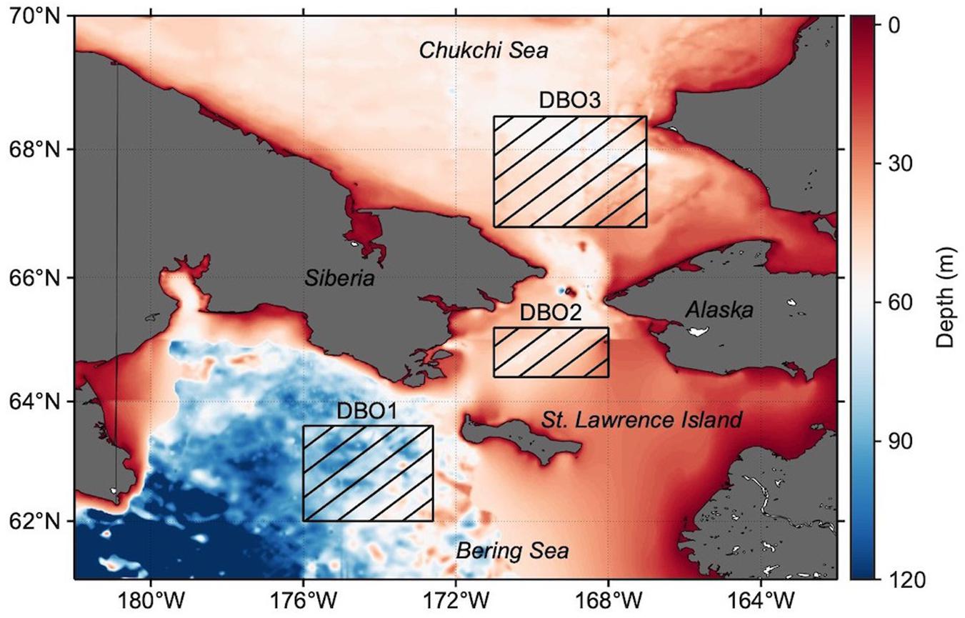
Figure 1. Bathymetry map of the Pacific Arctic, with the Distributed Biological Observatory (DBO) sites studied marked as hatched boxes: DBO1, near the St. Lawrence Island polynya region (62°N–63.6°N, 172.6°W–176°W); DBO2, located in the Chirikov Basin (64.4°N–65.2°N, 168°W–171°W); and DBO3, located in the southeastern Chukchi Sea (66.8°N–68.5°N, 167°W–171°W).
Time-Series Dataset
The level-3 daily standard mapped images of remote-sensing reflectance [Rrs(λ)] at 9 km spatial resolution at eight wavelengths (λ = 412, 443, 469, 488, 531, 547, 555, and 667 nm), derived by the Moderate Resolution Imaging Spectroradiometer (MODIS) sensor onboard the Aqua satellite, were downloaded from NASA’s Ocean Color website1, for the period 2003–2017. In addition, daily sea-ice concentrations gridded at 25-km resolution, which were derived by the Special Sensor Microwave/Imager (SSMI) and Special Sensor Microwave Imager/Sounder (SSMIS) onboard the Defense Meteorological Satellite Program (DMSP) (satellites DMSP-F13 and DMSP-F17, respectively), using an enhanced NASA Team algorithm (Markus and Cavalieri, 2000), were obtained from the National Snow and Ice Data Center (NSIDC) for the years 2003–2017. To align the spatial resolution of satellite data used in this study, daily sea-ice concentrations were resampled into 9-km resolution using nearest-neighbor interpolation (Perrette et al., 2011).
Phytoplankton Biomass and Size Structure
Chlorophyll-a (chla) concentration, which is a proxy of phytoplankton biomass, was computed from Rrs(λ) using the Arctic-OC3L algorithm developed and validated in the Chukchi Sea (Lewis et al., 2016). The Arctic-OC3L is a linear equation of the form:
where the coefficients a and b are empirically derived values and R is the base-10 logarithm of the maximum band ratio of Rrs(λ) for blue to green wavelengths.
In addition, the size structure of phytoplankton communities was detected using a chla size distribution (CSD) model (Waga et al., 2017, 2019) which retrieves the exponent of the CSD (hereafter, the CSD slope) as an index of the synoptic size structure of phytoplankton communities. A large CSD slope indicates a large proportion of smaller phytoplankton, whereas a small CSD slope suggests that larger phytoplankton dominate. The CSD model uses the spectral features of phytoplankton absorption coefficient [aph(λ)]. Note that the modified version of the quasi-analytical algorithms (Fujiwara et al., 2016) was applied to Rrs(λ) to derive aph(λ). To capture the spectral features of the aph(λ), a principle component analysis (PCA) was applied to normalized aph(λ) []. The formula for is given as:
Where mean[aph(λ)] and std[aph(λ)] are the wavelength mean and the standard deviations of aph(λ), respectively. The input values for the PCA comprised a matrix (m × N) constituted to , where m and N are the numbers of the wavelengths and the samples, respectively.
The resulting principle component (PC) scores were used to build a logistic-type regression function capturing the relationship between the CSD slope and variances of as:
where wi,j, and β0 are the loading factors for the ith PC score, the value at wavelength j, and the regression coefficients, respectively. Finally, the CSD slope is derived from Eq. (3) using the model parameters β0 and Cj.
Fall-Bloom Detection
Presence or absence of chla peaks in fall was determined by modeling time-series of daily chla over the post-bloom period on a pixel-per-pixel basis. The method used in this study was largely based on the method described in Ardyna et al. (2014) and Marchese et al. (2017). Prior to modeling chla, a local weighted scatterplot smoothing function was applied to chla time-series for avoiding biases from possible outliers. In addition, this study defined that a minimum of one chla value every 20 days and a minimum of six chla values over the entire post-bloom period were required to ensure valid representation of the time-series variation in chla at a given location (Ardyna et al., 2014). Finally, a chla time-series during the post-bloom period was modeled as a Gaussian function as follows:
where t represents the date; chla0 is the background chla; chlam is the amplitude of the chla peak observed at the date tm; and σ corresponds to the temporal width of the chla peak. The significance of the model was tested to the significance level of 5% (Ardyna et al., 2014). We defined the presence of a fall peak in chla, indicating the occurrence of a fall bloom, when the model was statistically significant (p < 0.05). Initial values of the parameters in Eq. (5) are shown in Table 1. The bloom duration was defined as the period between the bloom start and end: the bloom start was determined as the date at which the fitted chla reached 20% of its maximum amplitude (Marchese et al., 2017); the bloom end was defined as the date at which the fitted chla was below 20% of its maximum amplitude after the bloom start. In the case that the model was statistically insignificant (p ≥ 0.05), the absence of a fall peak in chla, indicating the absence of a fall bloom, was defined, and then identified as a straight line with a single term of chla0. We computed the occurrence of a fall bloom as a percentage of the years in which a chla peak in fall was detected to the years satisfying the criteria for modeling seasonal variation in chla (i.e., a minimum of one chla value every 20 days and a minimum of six chla values over the entire post-bloom period).
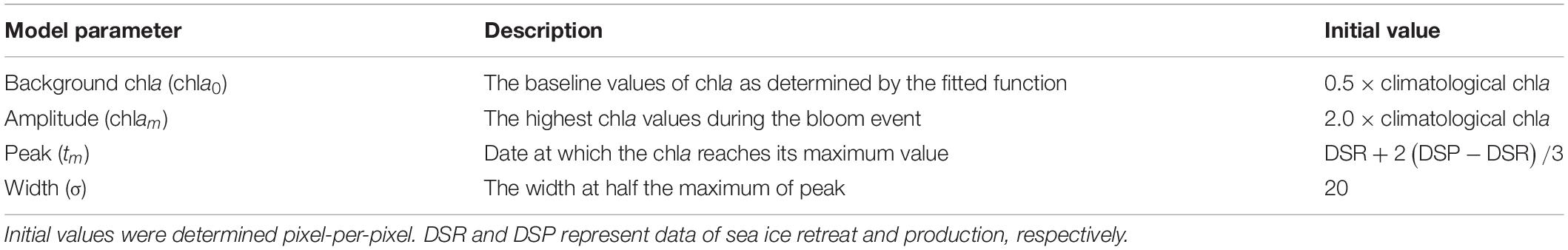
Table 1. Initial values of model parameters in fitting analysis (Eq. 5).
As a sea-ice-associated spring bloom generally lasts approximately 2 weeks (Niebauer et al., 1995), 2 weeks from the date of sea-ice breakup was termed as a spring-bloom period and was omitted from the modeling of time-series chla. In addition, a period after the date of sea-ice freeze-up was also removed from the modeling process. Here, the dates of sea-ice breakup and freeze-up were defined as the date on which a pixel registered two consecutive days below and above a 15% sea ice concentration, where we defined the breakup period as March 15–September 15 and the freeze-up period as September 15–March 15 (Frey et al., 2015). Thus, a post-bloom period was defined as the period between the end of the spring-bloom period and the date of sea-ice freeze-up.
Sensitivity Analysis for Fall-Bloom Detection
In the Arctic Ocean, clouds can affect ocean-color data availability and estimates, and in turn may disturb the modeling of seasonal variations in phytoplankton communities. To ensure robustness of our method for fall-bloom detection, we conducted a sensitivity analysis using the minimum number of data which satisfy the criteria. We subsampled a complete dataset of daily chla values to randomly create datasets that each included just six chla values with a minimum one chla value every 20 days.
We repeated this procedure for 100 trials, and then compared the resulting bloom characteristics with those captured by the original dataset. In addition, to examine how many data are required to retrieve stable values in the fall-bloom characteristics, we repeated the procedure for 100 trials at 5-data increment steps and then computed the coefficient of variance for each resulting fall-bloom characteristic. The complete dataset we used for this analysis was the daily averaged chla time-series over the pixels with a chla peak in fall within the boundary box of the DBO3 site (Figure 1) in 2003.
Results
Robustness of Fall-Bloom Detection
Figure 2 and Table 2 show the results of our sensitivity analysis. The sample dataset has 181 chla values in total, with a significant chla peak in fall. If we applied the Gaussian function to the sample dataset, the presence of a chla peak in fall was successfully captured by the model, and the resulting fall-bloom characteristics were exactly the same throughout the 100 trials (Table 2, model-1). In addition, we conducted the same procedure on the randomly selected six chla values with a minimum one chla value every 20 days. Although the presence of a fall bloom was ensured for more than half of the trials (Table 2, model-2), the rest showed an absence of a fall bloom probably because the assigned dataset didn’t contain chla values during the fall bloom period. Indeed, if we managed the dataset to contain at least one chla value during the fall bloom, the presence of a fall bloom increased to 98% (Table 2; model-3). However, model-detected fall-bloom characteristics showed huge variances if only a limited number of chla values were available for modeling the chla time-series. To obtain stable fall-bloom characteristics using our method, six chla values seem to be insufficient (Figure 3), while our sensitivity analysis demonstrated robustness for detecting the presence of a fall bloom if the time-series data contained valid chla values within the fall-bloom period.
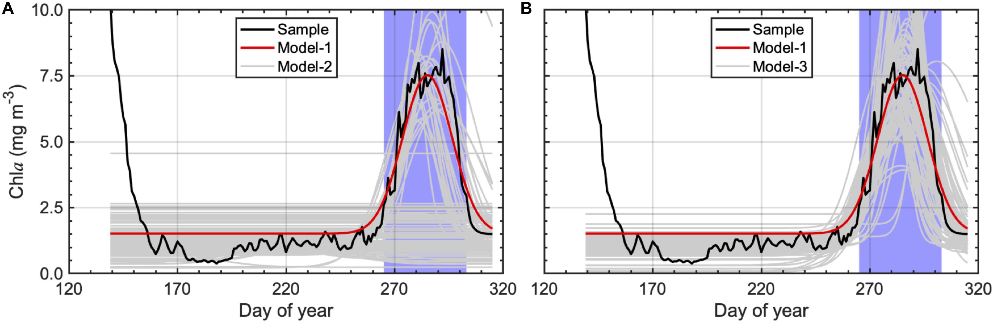
Figure 2. Gaussian fitting results using sample dataset, which was produced as daily averaged time-series over pixels with a chla peak in fall at the Distributed Biological Observatory (DBO) 3 site. Black lines represent time-series variations in sample dataset, and red lines show modeled chla variations based on fitting functions using entire sample dataset (model-1; N = 181). Gray lines indicate fitting results of (A) randomly selected chla values (model-2; N = 6) without any criteria and (B) randomly selected chla values (model-3; N = 6) containing at least one chla values during the fall bloom (blue-shaded areas).
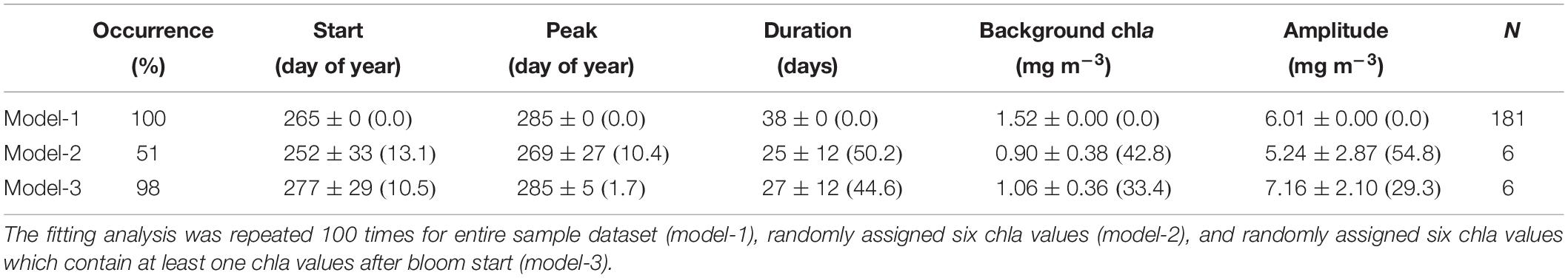
Table 2. Occurrence and characteristics of the fall bloom retrieved by the fitting analysis; average ± standard deviation (coefficient of variance).
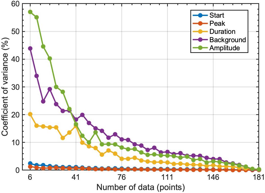
Figure 3. Relationships between number of data used for fitting analysis and coefficient of variance for fall-bloom characteristics. Fitting analysis was repeated for 100 times at 5-data increment steps between six and 181, and then computed coefficient of variance for each resulting fall-bloom characteristics.
Biomass and Size Structure of the Phytoplankton Community
The climatological values of chla and CSD slope during the post-bloom period were averaged for 2003–2017 (Figure 4). As a lower CSD slope indicates larger phytoplankton size structure, the patterns in the chla and CSD slope suggest that higher chla is consistent with larger phytoplankton size structure, and vice versa. Chla was high around the Bering Strait (Figure 4a). The resulting regionally averaged values of chla were highest for DBO2 (2.66 ± 0.12 mg m–3), followed by DBO3 (1.80 ± 0.20 mg m–3), and DBO1 (0.68 ± 0.07 mg m–3). In addition, we found specific coastal areas with high chla, such as at Norton Sound and Kotzebue Sound; however, these areas could encompass larger uncertainties mediated by inputs of terrestrial organic matter and sediments. In contrast, the CSD slope showed a clear inverse distribution to that of chla (Figure 4b): regional averaged values of CSD slope were lowest for DBO2 (1.54 ± 0.07), followed by DBO3 (1.85 ± 0.14), and DBO1 (1.93 ± 0.03).
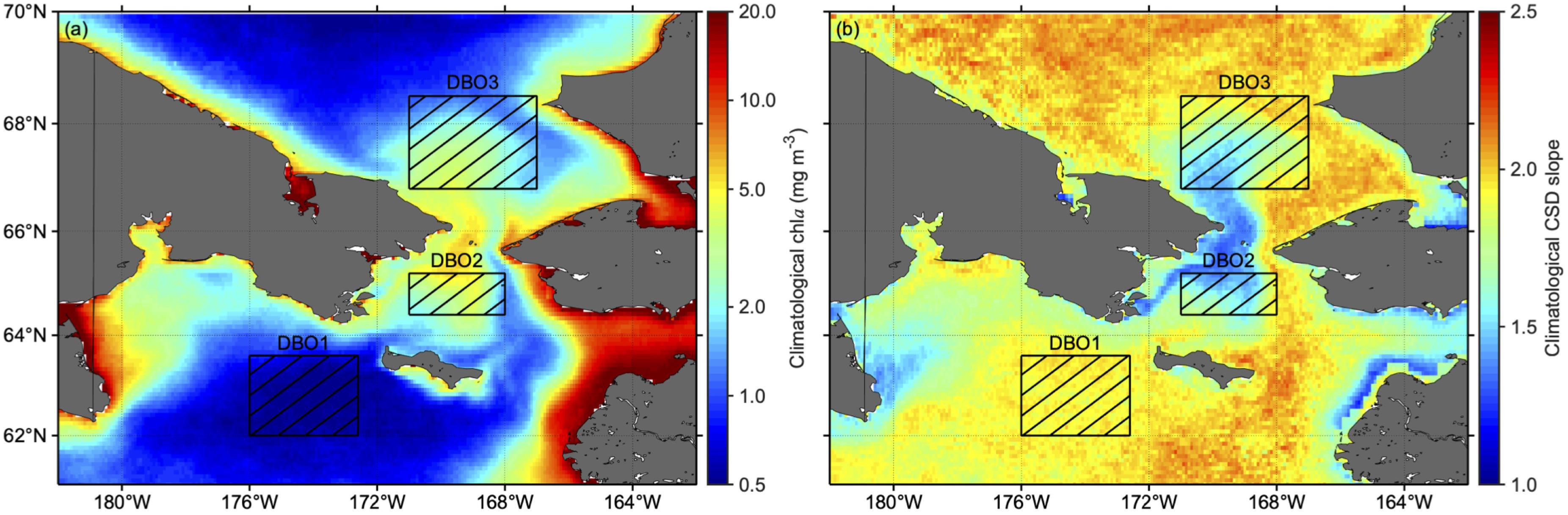
Figure 4. Spatial variations in climatology of (a) chla and (b) CSD slope during the post-bloom periods in the Pacific Arctic for 2003–2017.
Seasonal variations in climatological chla and CSD slope grouped by presence or absence of fall blooms are shown in Figure 5. Although fall-bloom detection was performed on a pixel-per-pixel basis, time-series data shown in Figure 3 were regionally averaged values collected on the same days of the year during 2003–2017 within each boundary box (Figure 1). The most important findings were the difference in CSD slope between presence and absence of fall blooms, and also a difference between “during fall blooms” and before/after the fall-bloom period (Figures 5d–f). When comparing the climatological CSD slope during the post-bloom period for the same day of the year between presence and absence of fall blooms, lower values of CSD slope were found for presence of fall blooms throughout all the DBO sites (Wilcoxon signed-rank test, p < 0.05). Furthermore, based on fitting the result of seasonal variations in chla accompanying afall bloom at the DBO sites (Figures 5a–c; Table 3), we compared the difference in the CSD slope during the fall-bloom period, and the CSD slope during the post-bloom period excepting the fall-bloom period: the CSD slope showed apparent lower values during the fall bloom than those values observed before and after the fall bloom (Mann–Whitney U test, p < 0.05). This result clearly suggests that the fall bloom is composed of large-celled phytoplankton. Note that maximum chla (Figures 5a–c) and minimum CSD slope (Figures 5d–f) were observed in spring for the DBO sites; these values would represent remnants of the sea-ice-associated spring bloom, which consisted of a higher biomass and larger size structure of the phytoplankton community as compared with those of a fall bloom. We ensured that there was no significant difference in chla during the spring-bloom period between presence and absence of fall blooms (Mann–Whitney U test, DBO1: p = 0.18; DBO2: p = 0.72; DBO3: p = 0.29).
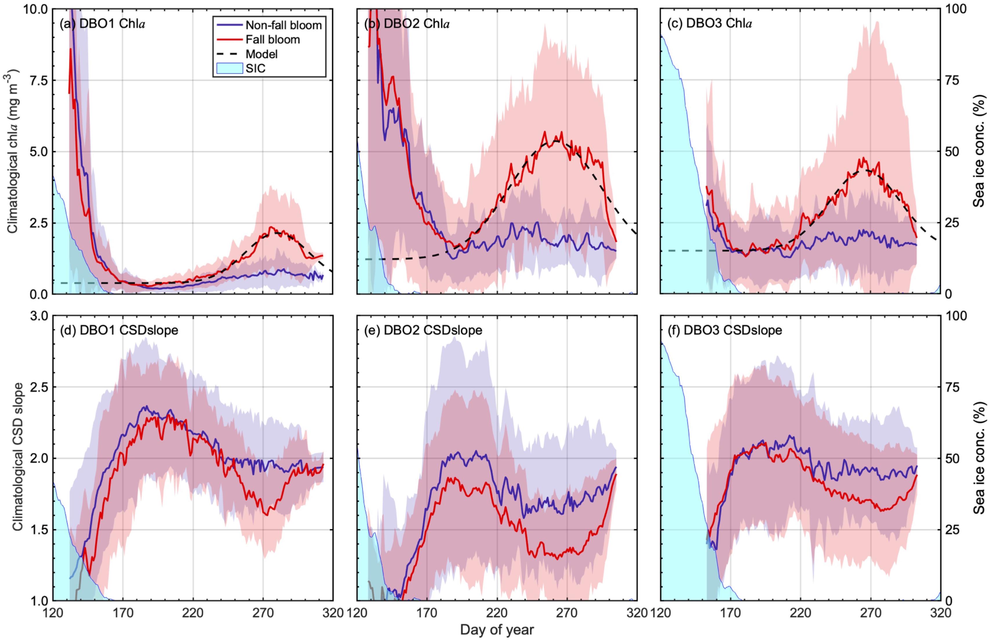
Figure 5. Seasonal variations in climatological (a–c) chla and (d–f) CSD slope with sea-ice concentration at three Distributed Biological Observatory (DBO) sites: (a,d) DBO1, (b,e) DBO2, and (c,f) DBO3. Red lines and shaded areas represent the average and standard deviations for regions where fall blooms were detected; blues lines represent the average and standard deviations for regions without fall blooms. Black dashed lines indicate modeled chla variations using climatological chla values grouped into presence of fall bloom. Climatological values of daily sea-ice concentration are shown as light blue areas.
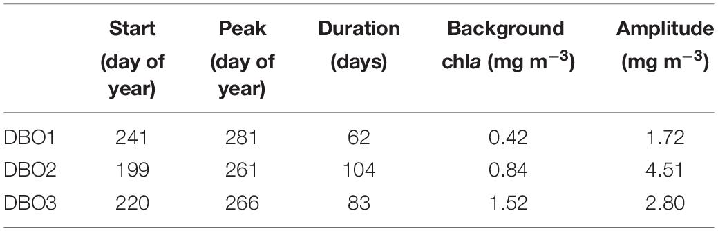
Table 3. Fall-bloom characteristics retrieved from seasonal time-series of climatological chla at the three distributed biological observatory (DBO) sites.
Occurrence of Fall Bloom
On average, ∼80% of pixels within each DBO site satisfied the criteria for modeling seasonal variation in chla (Table 4). In addition, the average number of available data during the post-bloom period across the DBO sites was 24 ± 6 points, which was apparently beyond our minimum criteria of six (Table 4). When we computed the fraction of the number of fall-bloom observed years to the total number of years satisfying the criteria on a pixel-per-pixel basis, frequent occurrences of fall blooms were detected in a wide area of the Pacific Arctic (Figure 6c). However, the west of St. Lawrence Island around the DBO1 showed infrequent occurrences of fall blooms. In addition, the regions displaying higher chla values, such as the Bering Strait, Norton Sound, and Kotzebue Sound, exhibited less frequent occurrences of fall blooms or negligible time-series variation when compared with adjacent regions. The resulting spatial variations in averaged occurrence of fall blooms are shown in Table 4; among the three DBO sites, DBO3 in the southeastern Chukchi Sea showed the highest proportion of fall blooms, at 40.6 ± 17.4% (cf. DBO1: 24.8 ± 13.1%; DBO2: 33.0 ± 12.4%).
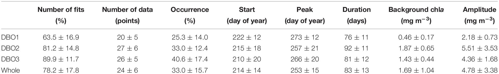
Table 4. Climatological fall-bloom characteristics for 2003–2017 at each distributed biological observatory (DBO) site and across the DBO sites; average ± standard deviation.
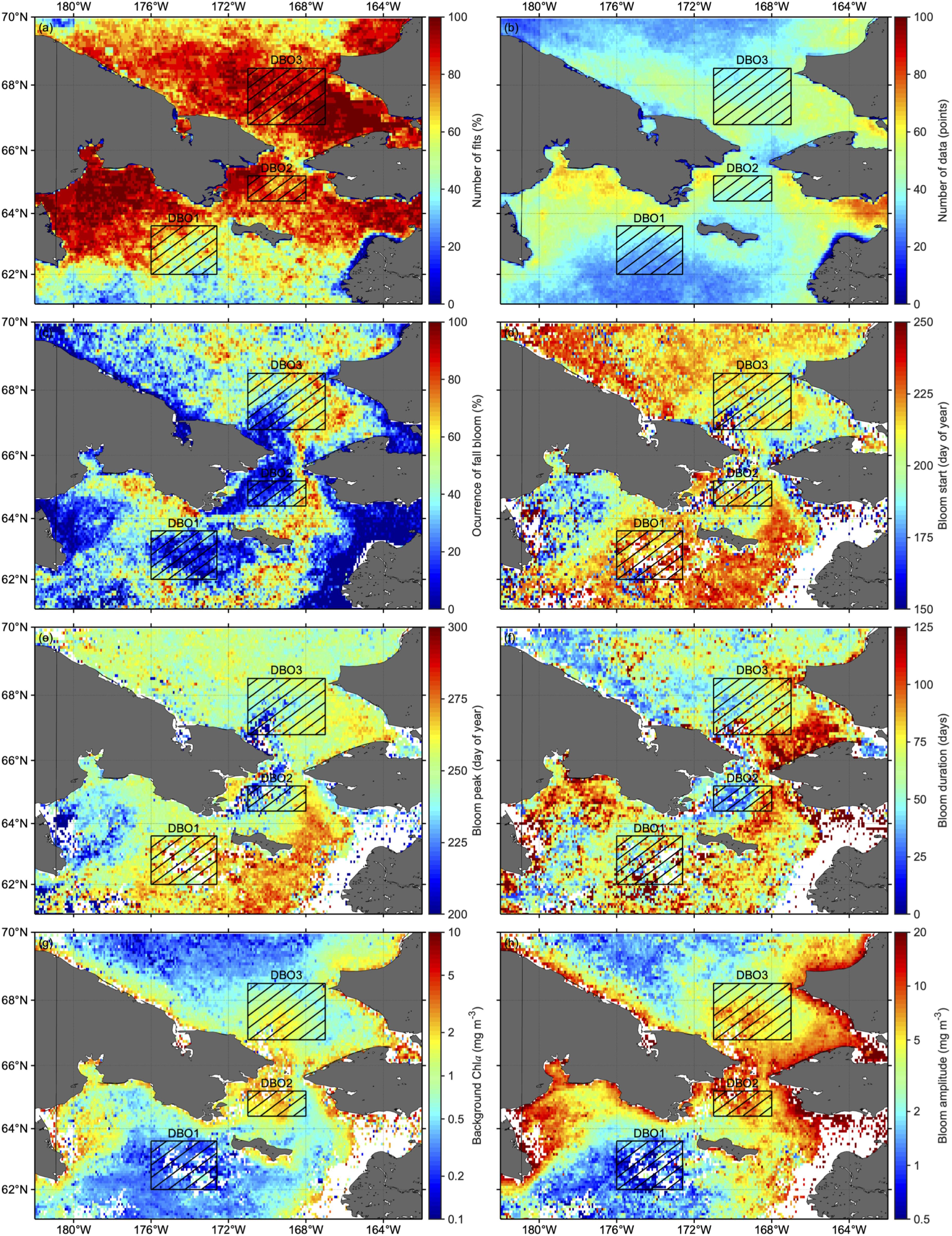
Figure 6. Climatology maps of (a) number of fits, (b) number of data, (c) occurrence of fall blooms, (d) bloom starts, (e) bloom peaks, (f) bloom durations, (g) background chla, and (h) bloom amplitudes in the Pacific Arctic. The number of fits is expressed as a percentage and derived as a ratio of the number of years that satisfied our criteria to the total number of years considered (i.e., 15 years). In addition, occurrence of fall blooms is expressed as percentages and computed as a ratio of years that fall blooms occurred within the number of years that satisfied our criteria. White represents areas where fall blooms were not detected for 2003–2017.
Temporal trends in the regional proportion of fall-bloom occurrences within the DBO sites, over the period 2003–2017, are shown in Figure 7c; two of the sites (DBO1 and DBO3) were identified as exhibiting statistically significant trends (Mann-Kendall test, p < 0.05). Positive trends in the occurrence of fall blooms were found for site DBO3, whereas a negative trend was observed for site DBO1, located near the St. Lawrence Island polynya region; in contrast, site DBO2 in the Chirikov Basin showed insignificant trends. The occurrence of fall blooms at DBO1 showed a drastic reduction over the study period: a fall bloom was detected in 47.3% of pixels within the DBO1 in 2003, whereas occurrences at this site dropped to 10.2% in 2017. Note that we ensured that temporal variations in occurrence of fall bloom at the DBO sites were not influenced by number of fits (Spearman’s rank correlation test, DBO1: p = 0.32; DBO2: p = 0.18; DBO3: p = 0.67) (Figure 6a) or number of available data for fitting analysis (Spearman’s rank correlation test, DBO1: p = 0.10; DBO2: p = 0.77; DBO3: p = 0.55) (Figure 6b). Accompanying such variations in occurrence of fall bloom at the DBO sites, average CSD slope during the post-bloom period at the DBO1 and DBO3 showed significant decreasing and increasing trends for 2003–2017 (Mann-Kendall test, p < 0.05) (Figure 8), respectively, whereas the DBO2 exhibited an insignificant trend over the study period (Mann-Kendall test, p = 0.28) (Figure 8). Indeed, there were statistically significant relationships between the CSD slope during the post-bloom period and occurrence of fall bloom at the three DBO sites (Spearman’s rank correlation test, p < 0.05). Consequently, we found an interesting spatial difference in temporal trends in occurrences of fall blooms associated with variations in phytoplankton size structure among the three DBO sites.
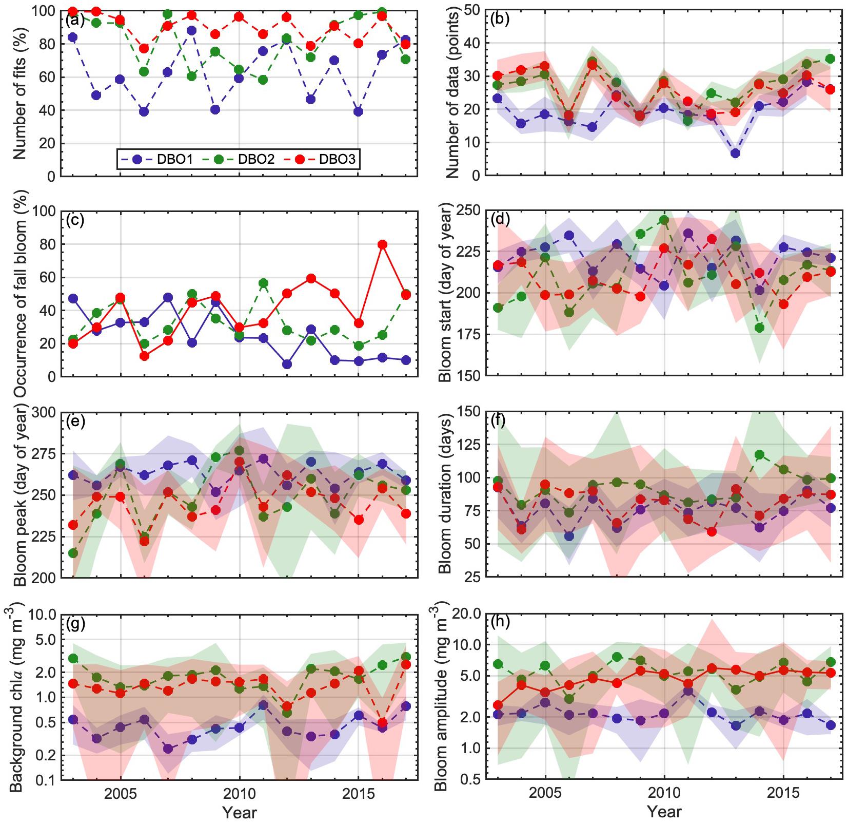
Figure 7. Interannual variations in the (a) number of fits, (b) number of data, (c) occurrences of fall blooms, (d) bloom starts, (e) bloom peaks, (f) bloom durations, (g) background chla, and (h) bloom amplitudes, at each of three Distributed Biological Observatory sites (DBO1–3), for 2003–2017. Number of fits is expressed as a percentage and was derived as a ratio of the number of years that satisfied our criteria to the total number of years considered (i.e., 15 years). In addition, the occurrence of fall blooms is expressed as a percentage and computed as a ratio of years when fall blooms occurred among the number of years that satisfied our criteria. Lines and shaded areas represent the average and standard deviation, respectively. Solid and dashed lines indicate significant (p < 0.05) and insignificant (p ≥ 0.05) temporal trends, respectively.
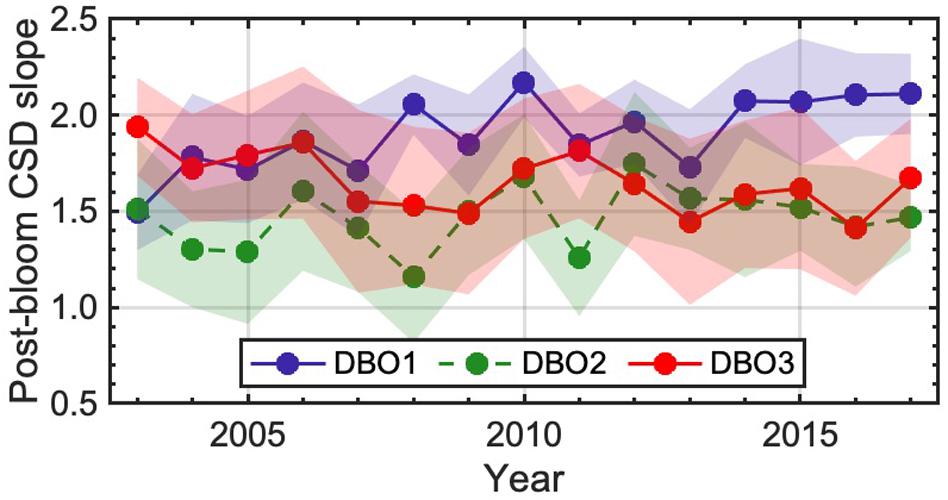
Figure 8. Interannual variation in the CSD slope during the post-bloom period at three Distributed Biological Observatory sites (DBO1–3) for 2003–2017. Lines and shaded areas represent the average and standard deviation, respectively. Solid and dashed lines indicate significant (p < 0.05) and insignificant (p ≥ 0.05) temporal trends, respectively.
Characteristics of the Fall Blooms
We examined spatial patterns of fall-bloom characteristics in the Pacific Arctic (Figures 6d–h). The fall blooms generally started in August (Table 4), although relatively earlier blooms were found in the Gulf of Anadyr (Figure 6d), and maximum values of chla were reached between mid-September and early October (Figure 6e). The duration of these fall blooms (Figure 6f) ranged from a minimum of two and a half months (DBO1: 76 ± 11 days) to a maximum of 3 months (DBO2: 92 ± 11 days) (Table 4). Spatial variations in background chla (Figure 6g) and bloom amplitude (Figure 6h) showed consistent spatial patterns: higher values were found on the western side of the Bering Strait and in coastal areas. It is noteworthy that bloom amplitude for site DBO1 was 2.18 ± 0.73 mg m–3, and was slightly higher than the background chla for site DBO2 (1.87 ± 0.65 mg m–3).
In summary, the fall bloom at DBO2 could be characterized as having the longest duration and the largest amplitude, as well as the highest level of background chla. A fall bloom with large amplitude for a longer duration was observed for site DBO3; by comparison, DBO1 exhibited a less-pronounced fall bloom owing to its small amplitude in addition to moderate duration. We also investigated interannual variations in fall-bloom characteristics for each DBO region. The amplitude showed a significant increasing trend at site DBO3, while none of the other fall-bloom characteristics exhibited a significant trend (Figures 7d–h). It is important to note that the characteristics of the fall blooms contain uncertainties due to the limited number of available chla values for the fitting analysis (Figure 3), although the fitting analysis for seasonal variations in chla was conducted using 24 ± 6 points on average (Table 4).
Discussion
Seasonal time-series variation in satellite-derived chla was modeled using a Gaussian function (Eq. 5) to distinguish whether a peak in chla was evident in fall. Evidently, our results depict the presence of fall blooms in a wide area of the Pacific Arctic (Figure 6c). It is noteworthy that relatively scarce occurrences of fall blooms were found in the regions with higher climatological chla values, such as the Bering Strait, Norton Sound, and Kotzebue Sound (Figure 4a). This result was ascribed to persistently high chla in these regions, which would prevent the detection of significant peaks during the post-bloom period. We found decreasing and increasing trends in the occurrence of a fall bloom at DBO1 and DBO3, respectively (Figure 7c), which significantly linked with interannual variation in phytoplankton size structure during the post-bloom period (Figure 8). Yokoi et al. (2016) reported a remarkable increase in the number of pennate diatoms during a small bloom in fall, supporting our results of a strong relationship between the size structure of the phytoplankton community and a fall bloom. As phytoplankton size structure during the post-bloom period strongly determines the amount of the flux of organic carbon into the sediment (Waga et al., 2019), interannual variations in phytoplankton size structure during the post-bloom period could influence not only the occurrence of a fall-bloom but also increased activity of higher trophic levels in the food web. Indeed, several studies have reported decreasing and increasing trends in benthic macrofaunal biomass at DBO1 and DBO3, respectively, while that of DBO2 showed an insignificant trend at DBO2 (Grebmeier et al., 2018; Waga et al., 2019).
Fall blooms are observed to occur more frequently in the Arctic Ocean during the last decade. In temperate regions, wind-driven mixing and the incidental upward nutrient supply trigger fall blooms (Chiswell et al., 2013), whereas the presence of sea ice prevents wind-driven mixing even during strong storms in the Arctic. However, the impact of storms on the upper ocean is becoming prominent due to a drastic increase in the ice-free period over the Arctic (Maksym, 2019). In fact, by modeling satellite-derived chla time series for 1998–2012, Ardyna et al. (2014) has reported that the pan-Arctic seems to be experiencing a fundamental shift in phytoplankton phenology from a polar (i.e., single bloom in spring) to a temperate mode (i.e., double blooms, in spring and fall) due to increased stormy days over ice-free waters in fall. Therefore, our finding of the increased occurrence of fall blooms at DBO3 over the years 2003–2017 might be explained by such atmospheric variations promoting an incidental upward nutrient supply from the region’s subsurface layer to the surface layer. Additionally, Danielson et al. (2017) suggested a positive relationship between nutrients in the southern part of the Chukchi Sea and a northward volume flux through the Bering Strait. The mean of the annual northward volume flux at the Bering Strait recorded a long-term increase of ∼0.01 Sv year–1 for the years 1990–2015, which is a remarkably large fraction of the recent climatological mean of 1.0 ± 0.05 Sv (Woodgate, 2018); hence, site DBO3, located in the southeastern Chukchi Sea, could over time receive more nutrients from the northern Bering Sea shelf. Furthermore, DBO3 has exhibited relatively weak water-column stratification, which allows upward nutrient flux from nutrient-rich bottom water to sun-lit surface water (Giesbrecht et al., 2019). Thus, the combined impact of these factors may be the cause of interannual variations in occurrences of fall blooms at DBO3.
The nutrient supply via wind-induced mixing is one of the most important factors related to biomass and size structure of the phytoplankton community in summer and fall on the Bering Sea shelf (Eisner et al., 2016); therefore, we expected that the increasing trend in numbers of stormy days in the Arctic (Ardyna et al., 2014) would promote the occurrence of fall blooms. However, temporal variations in the occurrence of fall blooms in DBO1 exhibited a decreasing trend for 2003–2017, with drastically low values after 2012 (Figure 7c). More specifically, occurrences of fall blooms in this region dropped from 47.3% in 2003 to 10.2% in 2017. Meanwhile, there is reasonable evidence of a significant reduction in the concentration of nutrients in bottom water between 2005 and 2016, presumably associated with bottom-water freshening of ∼1 psu near the M8 mooring site (62.194°N, 174.688°W) located in DBO1 as a consequence of warmer temperatures (Stabeno et al., 2019). This condition indicates that the decreased nutrient content in bottom water would not be able to trigger fall blooms in the DBO1 even if such water upwelled to the surface by wind-driven mixing. The bottom-water freshening would decrease the strength of vertical stratification, because the density gradient between the surface and bottom waters would decrease with bottom-water freshening (Ladd and Stabeno, 2012); nevertheless, our finding of the decreasing trend in occurrence of fall blooms at site DBO1 implies the primary importance of bottom-water nutrients rather than the frequency of wind-driven vertical mixing in this region. Furthermore, the impact of grazing from zooplankton on the phytoplankton standing stock could also contribute to the decreasing trend in occurrence of fall blooms at DBO1. Mesozooplankton responded to the increase in the large-celled phytoplankton during the fall bloom (Matsuno et al., 2015), and caused the effective removal of large-celled phytoplankton via selective grazing on larger phytoplankton (Fujiwara et al., 2018). Therefore, further investigation about interannual variations in zooplankton biomass and grazing impact on phytoplankton is essential to fully understand thedecreasing trends in occurrence of a fall bloom and the shift toward a smaller size structure of phytoplankton at the DBO2.
Occurrences of fall blooms at site DBO2 showed an insignificant trend during 2003–2017 (Figure 7c). Two factors might explain this. First, site DBO2 is located in the Chirikov Basin, between DBO1 and DBO3. Thus, the decreasing and increasing trends noted for sites DBO1 and DBO3, respectively, would collapse such trends, and, accordingly, DBO2 would show insignificant interannual variations. Second, site DBO2 is situated at the boundary of various water masses: i.e., Anadyr Water, Alaska Coastal Water, and Bering Shelf Water (Coachman et al., 1975). As the flow pathways of these water masses largely fluctuate owing to atmospheric forcing (Danielson et al., 2012, 2014), the incidental water-mass distribution in DBO2 could determine occurrences of fall blooms in this region. Overall, additional evidence is required to fully understand interannual variation in the occurrence of fall blooms at site DBO2.
In the eastern Bering Sea, the magnitudes of spring and fall blooms were significantly linked to each other, based on an analysis of mooring data (Sigler et al., 2014), possibly because the fraction of spring-bloom organic matter in the sediment is remineralized (Mordy et al., 2017) and then reintroduced to the euphotic zone during convection in the fall (Abe et al., 2019). Arctic shelves remineralize organic carbon in the sediment as efficiently and as rapidly as those at lower latitudes, despite the permanently low temperatures (Grebmeier and McRoy, 1989). Likewise, the bottom depths at our target regions were the same or shallower than depths in the eastern Bering Sea, and hence the influence of remineralized nutrients on the euphotic layer in fall would be substantial. However, values of average chla did not differ significantly for the spring-bloom period when comparing between data for the presence or absence of a fall bloom; this suggests why, in this study, a robust relationship was not found between the spring and fall blooms. A possible reason for the missing linkage between the spring and fall blooms in this study is limitation of the satellite remote-sensing capacity; that is, a presence of sea ice and extensive cloudiness obstructs satellite monitoring of the phytoplankton community (Marchese et al., 2017). Meanwhile, several studies have reported under-ice blooms in substantial portions of the Pacific Arctic during the last decade (Arrigo et al., 2012; Lowry et al., 2014). Therefore, the spring-bloom period, which was defined as the 14-day period from the date of sea-ice retreat, was possibly a period encompassing remnants of the spring bloom, and thus the actual spring-bloom period would have occurred prior to the bloom period defined in this study.
This study demonstrated spatiotemporal patterns in the occurrence of fall blooms associated with variations in phytoplankton size structure in the Pacific Arctic for 2003–2017. The Arctic has recently experienced drastic changes in sea ice dynamics that are driving variations in marine organisms (Grebmeier, 2012). In the Pacific Arctic food webs, even small changes in the lower trophic levels would have an influence on the distribution and abundance of higher trophic levels as a consequence of the short and efficient energy-transfer pathways (Grebmeier et al., 2010), and thus the bottom-up control on higher trophic levels is crucial (Schonberg et al., 2014). This study revealed an increased occurrence of fall blooms, which has the potential to explain recent variations in benthic macrofaunal biomass at the DBO sites (Grebmeier et al., 2018; Waga et al., 2019). Consequently, our findings contribute to facilitate an holistic understanding of ocean dynamics and complex trophic linkages from primary production to higher trophic levels, and improve our understanding of processes causing variations within marine ecosystems, as might occur in the Pacific Arctic.
Author’s Note
The ocean-color data were produced and distributed by the NASA’s Distributed Active Archive Center at the Goddard Space Flight Center. Sea-ice-concentration data were provided by the National Snow and Ice Data Center at the University of Colorado.
Data Availability Statement
The datasets generated for this study are available on request to the corresponding author.
Author Contributions
HW analyzed the data, organized, prepared and wrote the first version of the manuscript, and prepared all figures and tables. TH contributed to writing the final version of the manuscript.
Funding
This study was supported by the Arctic Challenge for Sustainability (ArCS) Project, funded by the Ministry of Education, Culture, Sports, Science, and Technology of Japan (MEXT).
Conflict of Interest
The authors declare that the research was conducted in the absence of any commercial or financial relationships that could be construed as a potential conflict of interest.
Footnotes
References
Abe, H., Sampei, M., Hirawake, T., Waga, H., Nishino, S., and Ooki, A. (2019). Sediment-associated phytoplankton release from the seafloor in response to wind-induced barotropic currents in the bering strait. Front. Mar. Sci. 6:243. doi: 10.3389/fmars.2019.00097
Ardyna, M., Babin, M., Gosselin, M., Devred, E., and Tremblay, J. -É (2014). Recent Arctic Ocean sea ice loss triggers novel fall phytoplankton blooms. Geophys. Res. Lett. 41, 6207–6212. doi: 10.1002/2014GL061047
Arrigo, K. R., Perovich, D. K., Pickart, R. S., Brown, Z. W., van Dijken, G. L., Lowry, K. E., et al. (2012). Massive phytoplankton blooms under arctic sea ice. Science 336, 1408–1408. doi: 10.1126/science.1215065
Arrigo, K. R., van Dijken, G., and Pabi, S. (2008). Impact of a shrinking Arctic ice cover on marine primary production. Geophys. Res. Lett. 35:L19603. doi: 10.1029/2008GL035028
Chiswell, S. M., Bradford-Grieve, J., Hadfield, M. G., and Kennan, S. C. (2013). Climatology of surface chlorophyll a, autumn-winter and spring blooms in the southwest Pacific Ocean. J. Geophys. Res. Oceans 118, 1003–1018. doi: 10.1002/jgrc.20088
Coachman, L. K., Aagaard, K., and Tripp, R. B. (1975). Bering Strait: The Regional Physical Oceanography. Seattle: University of Washington Press.
Cole, H., Henson, S., Martin, A., and Yool, A. (2012). Mind the gap: the impact of missing data on the calculation of phytoplankton phenology metrics. J. Geophys. Res. 117:C08030. doi: 10.1029/2012JC008249
Comiso, J. C. (2012). Large decadal decline of the Arctic multiyear ice cover. J. Clim. 25, 1176–1193. doi: 10.1175/JCLI-D-11-00113.1
Danielson, S., Weingartner, T., Aagaard, K., Zhang, J., and Woodgate, R. (2012). Circulation on the central Bering Sea shelf, July 2008 to July 2010. J. Geophys. Res. 117:C10003. doi: 10.1029/2012JC008303
Danielson, S. L., Eisner, L., Ladd, C., Mordy, C., Sousa, L., and Weingartner, T. J. (2017). A comparison between late summer 2012 and 2013 water masses, macronutrients, and phytoplankton standing crops in the northern Bering and Chukchi Seas. Deep Sea Res. II 135, 7–26. doi: 10.1016/j.dsr2.2016.05.024
Danielson, S. L., Weingartner, T. J., Hedstrom, K. S., Aagaard, K., Woodgate, R., Curchitser, E., et al. (2014). Coupled wind-forced controls of the Bering–Chukchi shelf circulation and the Bering Strait throughflow: ekman transport, continental shelf waves, and variations of the Pacific–Arctic sea surface height gradient. Prog. Oceanogr. 125, 40–61. doi: 10.1016/j.pocean.2014.04.006
Eisner, L. B., Gann, J. C., Ladd, C. D., Cieciel, K., and Mordy, C. W. (2016). Late summer/early fall phytoplankton biomass (chlorophyll a) in the eastern Bering Sea: spatial and temporal variations and factors affecting chlorophyll a concentrations. Deep Sea Res. II 134, 100–114. doi: 10.1016/j.dsr2.2015.07.012
Finkel, Z. V., Beardall, J., Flynn, K. J., Quigg, A., Rees, T. A. V., and Raven, J. A. (2009). Phytoplankton in a changing world: cell size and elemental stoichiometry. J. Plankton Res. 32, 119–137. doi: 10.1093/plankt/fbp098
Frey, K. E., Moore, G. W. K., Cooper, L. W., and Grebmeier, J. M. (2015). Divergent patterns of recent sea ice cover across the Bering, Chukchi, and Beaufort seas of the Pacific Arctic Region. Prog. Oceanogr. 136, 32–49. doi: 10.1016/j.pocean.2015.05.009
Fujiwara, A., Hirawake, T., Suzuki, K., Eisner, L., Imai, I., Nishino, S., et al. (2016). Influence of timing of sea ice retreat on phytoplankton size during marginal ice zone bloom period on the Chukchi and Bering shelves. Biogeosciences 13, 115–131. doi: 10.5194/bg-13-115-2016
Fujiwara, A., Nishino, S., Matsuno, K., Onodera, J., Kawaguchi, Y., Hirawake, T., et al. (2018). Changes in phytoplankton community structure during wind-induced fall bloom on the central Chukchi shelf. Polar Biol. 41, 1279–1295. doi: 10.1007/s00300-018-2284-7
Giesbrecht, K. E., Varela, D. E., Wiktor, J., Grebmeier, J. M., Kelly, B., and Long, J. E. (2019). A decade of summertime measurements of phytoplankton biomass, productivity and assemblage composition in the Pacific Arctic Region from 2006 to 2016. Deep Sea Res. II 162, 93–113. doi: 10.1016/j.dsr2.2018.06.010
Grebmeier, J., Frey, K., Cooper, L., and Kêdra, M. (2018). Trends in benthic macrofaunal populations, seasonal sea ice persistence, and bottom water temperatures in the bering strait region. Oceanography 31, 136–151. doi: 10.5670/oceanog.2018.224
Grebmeier, J. M. (2012). Shifting patterns of life in the Pacific arctic and sub-arctic seas. Annu. Rev. Mar. Sci. 4, 63–78. doi: 10.1146/annurev-marine-120710-100926
Grebmeier, J. M., and McRoy, C. P. (1989). Pelagic-benthic coupling on the shelf of the northern Bering and Chukchi Seas. Ill Benthic food supply and carbon cycling. Mar. Ecol. Prog. Ser. 53, 79–91. doi: 10.3354/meps053079
Grebmeier, J. M., Moore, S. E., Overland, J. E., Frey, K. E., and Gradinger, R. (2010). Biological response to recent pacific Arctic sea ice retreats. EOS 91, 161–162. doi: 10.1029/2010EO180001
Kashiwase, H., Ohshima, K. I., Nihashi, S., and Eicken, H. (2017). Evidence for ice-ocean albedo feedback in the Arctic Ocean shifting to a seasonal ice zone. Sci. Rep. 7:8170. doi: 10.1038/s41598-017-08467-z
Ladd, C., and Stabeno, P. J. (2012). Stratification on the Eastern Bering Sea shelf revisited. Deep Sea Res. II 65-70, 72–83. doi: 10.1016/j.dsr2.2012.02.009
Lewis, K. M., Mitchell, B. G., van Dijken, G. L., and Arrigo, K. R. (2016). Regional chlorophyll a algorithms in the Arctic Ocean and their effect on satellite-derived primary production estimates. Deep Sea Res. II 130, 14–27. doi: 10.1016/j.dsr2.2016.04.020
Lowry, K. E., van Dijken, G. L., and Arrigo, K. R. (2014). Evidence of under-ice phytoplankton blooms in the Chukchi Sea from 1998 to 2012. Deep Sea Res. II 105, 105–117. doi: 10.1016/j.dsr2.2014.03.013
Maksym, T. (2019). Arctic and Antarctic sea ice change: contrasts, commonalities, and causes. Annu. Rev. Mar. Sci. 11, 187–213. doi: 10.1146/annurev-marine-010816-060610
Marchese, C., Albouy, C., Tremblay, J. -É, Dumont, D., d’Ortenzio, F., Vissault, S., et al. (2017). Changes in phytoplankton bloom phenology over the North Water (NOW) polynya: a response to changing environmental conditions. Polar Biol. 40, 1721–1737. doi: 10.1007/s00300-017-2095-2
Markus, T., and Cavalieri, D. J. (2000). An enhancement of the NASA Team sea ice algorithm. IEEE Trans. Geosci. Remote Sens. 38, 1387–1398. doi: 10.1109/36.843033
Matsuno, K., Yamaguchi, A., Nishino, S., Inoue, J., and Kikuchi, T. (2015). Short-term changes in the mesozooplankton community and copepod gut pigment in the Chukchi Sea in autumn: reflections of a strong wind event. Biogeosciences 12, 4005–4015. doi: 10.5194/bg-12-4005-2015
Moore, S. E., and Grebmeier, J. M. (2018). The distributed biological observatory: linking physics to biology in the Pacific Arctic Region. ARCTIC 71, 1–7. doi: 10.14430/arctic4606
Mordy, C. W., Devol, A., Eisner, L. B., Kachel, N., Ladd, C., Lomas, M. W., et al. (2017). Nutrient and phytoplankton dynamics on the inner shelf of the eastern Bering Sea. J. Geophys. Res. Oceans 122, 2422–2440. doi: 10.1002/2016JC012071
Niebauer, H. J., Alexander, V., and Henrichs, S. M. (1995). A time-series study of the spring bloom at the Bering Sea ice edge I. Physical processes, chlorophyll and nutrient chemistry. Cont. Shelf Res. 15, 1859–1877. doi: 10.1016/0278-4343(94)00097-7
Nishino, S., Kawaguchi, Y., Inoue, J., Hirawake, T., Fujiwara, A., Futsuki, R., et al. (2015). Nutrient supply and biological response to wind-induced mixing, inertial motion, internal waves, and currents in the northern Chukchi Sea. J. Geophys. Res. Oceans 120, 1975–1992. doi: 10.1002/2014JC010407
Perrette, M., Yool, A., Quartly, G. D., and Popova, E. E. (2011). Near-ubiquity of ice-edge blooms in the Arctic. Biogeosciences 8, 515–524. doi: 10.5194/bg-8-515-2011
Polyakov, I. V., Timokhov, L. A., Alexeev, V. A., Bacon, S., Dmitrenko, I. A., Fortier, L., et al. (2010). Arctic Ocean warming contributes to reduced polar ice cap. J. Phys. Oceanogr. 40, 2743–2756. doi: 10.1175/2010jpo4339.1
Schonberg, S. V., Clarke, J. T., and Dunton, K. H. (2014). Distribution, abundance, biomass and diversity of benthic infauna in the Northeast Chukchi Sea, Alaska: relation to environmental variables and marine mammals. Deep Sea Res. II 102, 144–163. doi: 10.1016/j.dsr2.2013.11.004
Sigler, M. F., Stabeno, P. J., Eisner, L. B., Napp, J. M., and Mueter, F. J. (2014). Spring and fall phytoplankton blooms in a productive subarctic ecosystem, the eastern Bering Sea, during 1995–2011. Deep Sea Res. II 109, 71–83. doi: 10.1016/j.dsr2.2013.12.007
Stabeno, P. J., Bell, S. W., Bond, N. A., Kimmel, D. G., Mordy, C. W., and Sullivan, M. E. (2019). Distributed biological observatory region 1: physics, chemistry and plankton in the northern Bering Sea. Deep Sea Res. II 162, 8–21. doi: 10.1016/j.dsr2.2018.11.006
Steele, M., Ermold, W., and Zhang, J. (2008). Arctic Ocean surface warming trends over the past 100 years. Geophys. Res. Lett. 35:67. doi: 10.1029/2007GL031651
Waga, H., Hirawake, T., Fujiwara, A., Grebmeier, J. M., and Saitoh, S.-I. (2019). Impact of spatiotemporal variability in phytoplankton size structure on benthic macrofaunal distribution in the Pacific Arctic. Deep Sea Res. II 162, 114–126. doi: 10.1016/j.dsr2.2018.10.008
Waga, H., Hirawake, T., Fujiwara, A., Kikuchi, T., Nishino, S., Suzuki, K., et al. (2017). Differences in rate and direction of shifts between phytoplankton size structure and sea surface temperature. Remote Sens. 9:222. doi: 10.3390/rs9030222
Woodgate, R. A. (2018). Increases in the Pacific inflow to the Arctic from 1990 to 2015, and insights into seasonal trends and driving mechanisms from year-round Bering Strait mooring data. Prog. Oceanogr. 160, 124–154. doi: 10.1016/j.pocean.2017.12.007
Keywords: Bering Sea, Chukchi Sea, satellite remote sensing, ocean color, post-bloom period, marine phytoplankton, spatiotemporal variation
Citation: Waga H and Hirawake T (2020) Changing Occurrences of Fall Blooms Associated With Variations in Phytoplankton Size Structure in the Pacific Arctic. Front. Mar. Sci. 7:209. doi: 10.3389/fmars.2020.00209
Received: 20 November 2019; Accepted: 17 March 2020;
Published: 21 April 2020.
Edited by:
Carol Robinson, University of East Anglia, United KingdomReviewed by:
Emmanuel Devred, Department of Fisheries and Oceans, CanadaVictoria Hill, Old Dominion University, United States
Jens Nielsen, National Oceanic and Atmospheric Administration, United States
Copyright © 2020 Waga and Hirawake. This is an open-access article distributed under the terms of the Creative Commons Attribution License (CC BY). The use, distribution or reproduction in other forums is permitted, provided the original author(s) and the copyright owner(s) are credited and that the original publication in this journal is cited, in accordance with accepted academic practice. No use, distribution or reproduction is permitted which does not comply with these terms.
*Correspondence: Hisatomo Waga, hwaga@alaska.edu