 Thijs Christiaan van Son1*
 Nikolaos Nikolioudakis2
 Henning Steen1
 Jon Albretsen1
 Birgitte Rugaard Furevik3,4Sigrid Elvenes5
 Frithjof Moy1
 Kjell Magnus Norderhaug1
- 1Institute of Marine Research, Arendal, Norway
- 2Institute of Marine Research, Bergen, Norway
- 3The Norwegian Meteorological Institute, Oslo, Norway
- 4Danish Meteorological Institute, Copenhagen, Denmark
- 5Geological Survey of Norway, Trondheim, Norway
Kelp forests are highly productive systems that are important ecologically and commercially as well as in a blue carbon perspective. Given their importance, there is an urgent need to achieve reliable estimates of the spatial distribution of their biomass. Species distribution modelling is a powerful tool for producing such estimates, but it requires a solid framework, including important environmental covariates that have a direct effect on their biomass, a proper sampling strategy, and an independent evaluation dataset. Using Laminaria hyperborea as a model species, we developed a modelling framework considering these requirements and necessary steps to produce reliable predictions. Our modelling framework included proportion of hard substrate and bottom wave exposure, both crucial covariates that have a direct effect on the biomass of L. hyperborea, but rarely included in modelling studies. Furthermore, we devised a sampling strategy with field observations covering the whole environmental covariate space present in the study area. Subsequently, we fitted GAMs relating the field observations of the biomass of L. hyperborea to relevant environmental covariates. The best model containing the predictors bottom wave exposure, depth, and proportion hard substrate explained most of the variance in the dataset (83.1% deviance explained). This model was then used to predict the spatial distribution of biomass across the whole study area. To assess the reliability of the biomass predictions, we used an independent dataset of L. hyperborea biomass observations from the same area. This independent dataset correlated very well with spatial predictions of biomass based on our best model (R = 0.85). In total, we predicted a biomass of 457,000 tonnes in a 1,150 km2 study area on the West coast of Norway. Our modelling framework provides the means for developing a biomass model on a broader geographical scale. Such a model will be invaluable in improving kelp management regimes as well as for estimating the contribution of kelp forests to ecosystem services such as carbon sequestration and climate budgets.
Introduction
Kelp forms dense forests in shallow coastal areas from mid- to high latitudes around the world (Steneck et al., 2002). These forests are among the highest productive ecosystems on the planet and provide a variety of ecosystem services (Vilalta-Navas et al., 2018). Only a small part, less than 10%, of the kelp production is consumed inside the kelp forests. The rest is exported as small and large kelp fragments and fuels ecosystems in shallow and deep waters (Norderhaug and Christie, 2011). Hence, as these processes have become more evident, the role of kelp in carbon sequestration has been highlighted and an unknown part of the kelp produced is buried in sediments on deep water (Krause-Jensen and Duarte, 2016).
The part of the production consumed within the kelp forest supports diverse and abundant communities of invertebrates and algae. The three-dimensional structure of the kelp forest creates a diverse habitat that nurses a wide range of fish species (Norderhaug et al., 2005) and provides feeding areas for seabirds and mammals (Bjørge et al., 1995; Lorentsen et al., 2010). Kelp forests are therefore regarded as important areas for the coastal fishery.
Kelp is harvested for the extraction of alginate, a thickener used in pharmaceutical and food industry. Managing and understanding the ecological importance of these ecosystem engineers should rely on firm knowledge about the resources available. However, basic knowledge about the biomass and distribution of this important resource is still lacking and such knowledge may reduce conflicts of interest between different stakeholders. Proper management of kelp resources requires detailed knowledge about their spatial biomass distribution. Only then will we be able to achieve reliable estimates of how the commercially harvested biomass compares to the standing stock and subsequently devise harvesting regimes within sustainable limits.
Studies that provide complete coverage of spatial predictions can potentially provide accurate and reliable estimates of the standing stock of a kelp species. In this regard, there exist studies on the spatial distribution of the probability of occurrence of kelp forests (Bekkby et al., 2009; Raybaud et al., 2013; Gregr et al., 2018), abundance (Young et al., 2015), and assemblages (Rattray et al., 2015). These studies provide valuable ecological insights but can only indirectly yield information about the standing stock of the kelp species of interest.
Two studies from France, however, developed statistical models of the biomass of Laminaria species and subsequently predicted the species’ distribution of biomass in space (Gorman et al., 2012; Bajjouk et al., 2015). This also allowed them to directly estimate the standing stock. The first step in obtaining good estimates of the standing stock of kelp in a given area is to attain reliable observations of the biomass of kelp. Attaining such observations of kelp biomass is labour intensive and time-consuming, often involving diving (e.g., Gorman et al., 2012). Remote sensing represents an alternative and potentially promising method (Cavanaugh et al., 2011; Nijland et al., 2019), but reliable estimates of the spatial distribution of kelp biomass will still to a large degree have to be based on statistical modelling based on direct observations.
The statistical model needs to include covariates that have a direct effect on the kelp biomass and field observations must be based on a proper sampling strategy that is able to cover the whole environmental covariate space. Then species distribution modelling (Guisan and Zimmermann, 2000) can provide means to accurately estimate the spatial distribution of biomass and subsequently the standing stock within a given area. However, without a proper sampling strategy covering the whole environmental covariate space, predictions to new data containing combinations of environmental covariates not covered by the sampling strategy will be unreliable (Elith and Leathwick, 2007).
Using Laminaria hyperborea as a model species, we used the principles above to model its spatial distribution of biomass in a pilot area on the west coast of Norway, where high resolution data on relevant environmental covariates were available. Laminaria hyperborea grows in exposed coastal areas along the whole coast of Norway (Sjøtun et al., 1993). It is both ecologically (Norderhaug et al., 2003; Teagle et al., 2017) and commercially important (Steen et al., 2016). Knowledge about how its biomass relates to structuring environmental processes and how its biomass is spatially distributed is crucial to further improve the current management regime. The purpose of this study is therefore threefold: (1) to identify important environmental covariates that control the biomass distribution of L. hyperborea and devise a sound sampling strategy based on these covariates; (2) to make predictions about the spatial distribution of L. hyperborea biomass based on the best statistical model; and (3) to apply an independent evaluation dataset to assess the reliability of the model and its spatial predictions.
Materials and Methods
Study Area and Field Sampling Method
Field sampling was conducted in April and June 2017 in the southern part of the county of Møre and Romsdal on the West coast of Norway (Figure 1). The extent of the study area is 1150 km2. Here we find some of the most exposed areas along the Norwegian coast, likely providing an optimal environment for kelp production and biomass build-up. The study area has a complex topography, encompassing numerous large and small islands. Western and northern parts of the area include shallow banks (0–100 m) open to the Norwegian Sea, while the steep-sided fjords of the southern part reach depths of 600 m and the eastern part comprises sheltered straits and basins of varying depth. Most importantly, available high-resolution bathymetry made this area optimal for developing a spatial distribution model for kelp biomass.
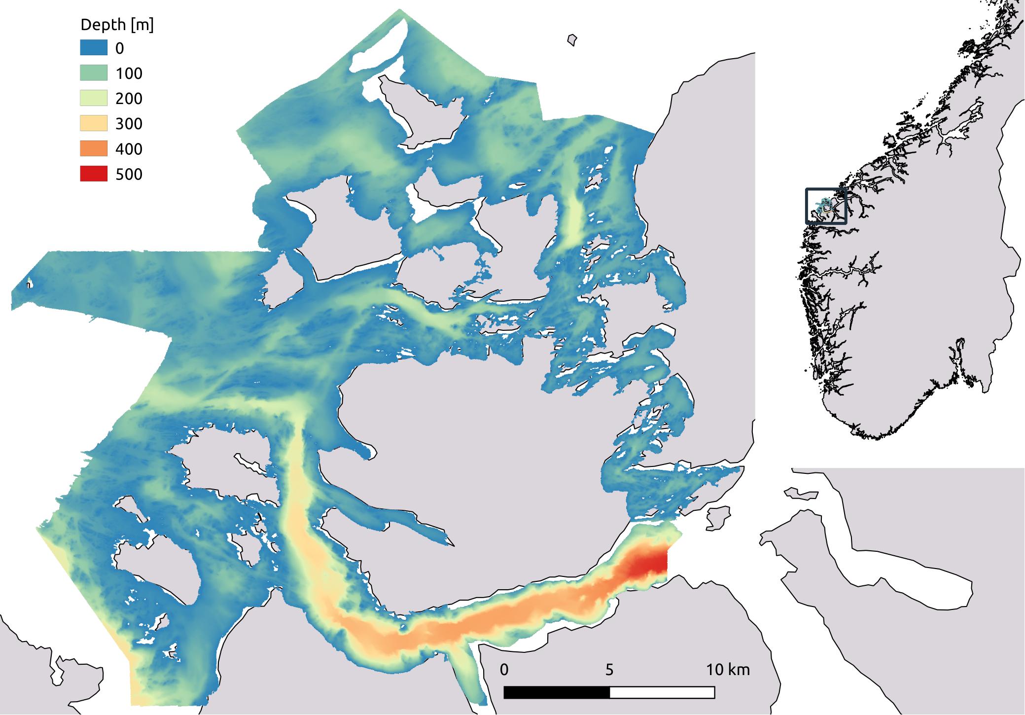
Figure 1. Map showing the geographical location and the extent of the study area as outlined by the bathymetry raster. The observations as well as the spatial predictions are limited to depths shallower than 35 m.
Sampling Strategy
The implemented sampling strategy covered as much as possible of the whole range of combinations of environmental gradients in the study area. The best way of thinking about this is to envision the ranges of covariates creating an n-dimensional space. A good sampling strategy is one that achieves a good representation of this n-dimensional space, which we can call the environmental covariate space. The quality of such a sampling strategy is dependent on the quality of each covariate, which is primarily dependent on two factors: (1) whether the covariate represents a direct or indirect effect on the response; and (2) how well the covariate represents its underlying environmental gradient. Consequently, a sampling strategy with a good representation of the environmental covariate space may still not sample the true environmental gradients adequately. Finally, all covariates to be used in the modelling should also be used in planning the sampling strategy.
Environmental Covariates
Four environmental covariates were used in the stratification process (Figure 2).
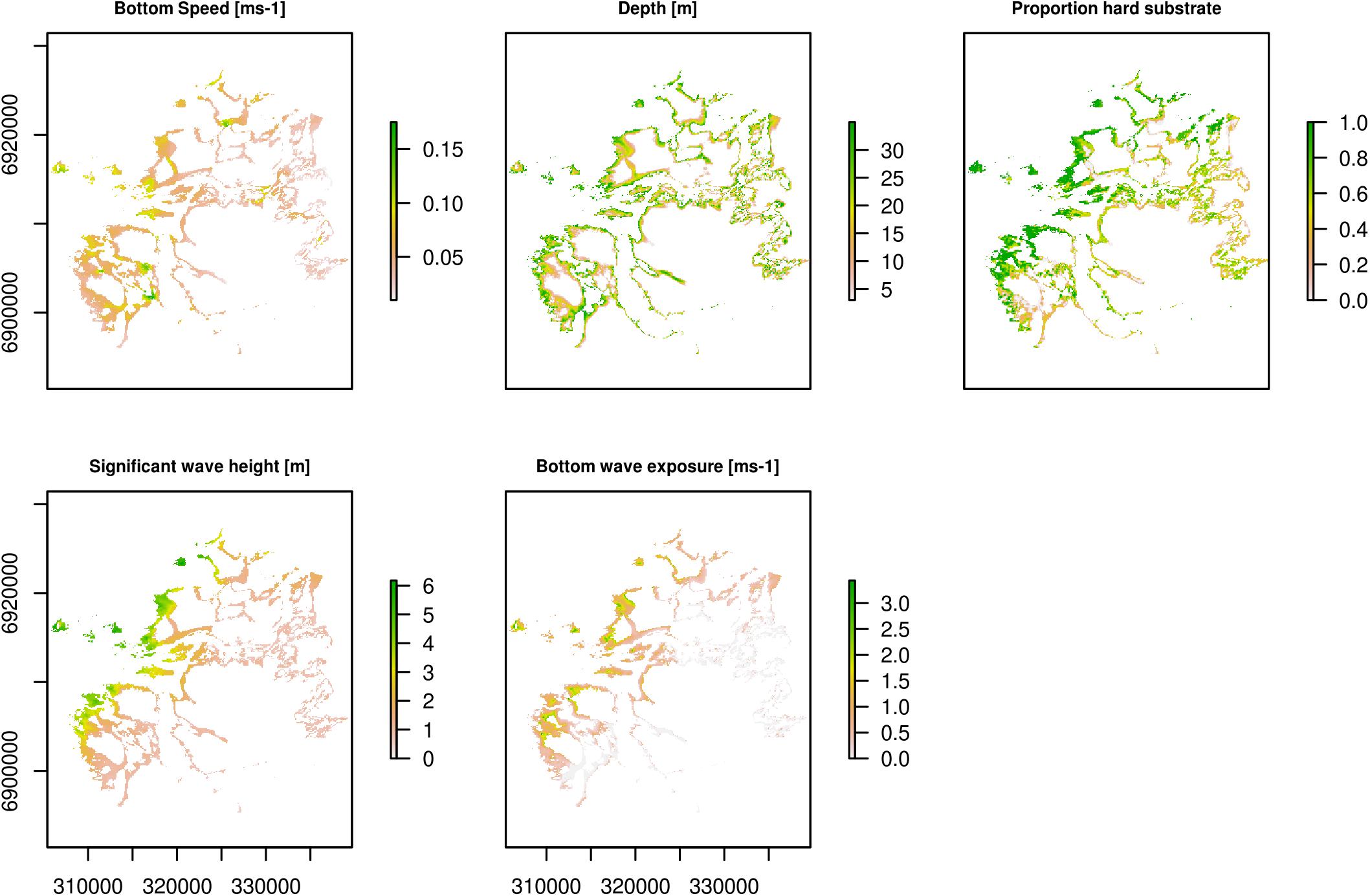
Figure 2. Raster plots of environmental covariates used in the fitted GAM models. Plots show values for areas shallower than 35 m. Coordinates in WGS84 UTM32N.
Depth
We used high resolution (2 m) bathymetry data acquired by the Norwegian Hydrographic Service (NHS). These data have been declassified by the Norwegian Defence Authorities and are available for public use, and they can be accessed at https://hoydedata.no/LaserInnsyn/.
Proportion hard substrate
The Geological Survey of Norway (NGU) has published a series of detailed marine base maps representing seabed sediment conditions of the study area (Elvenes et al., 2019). The maps are available at www.ngu.no and www.mareano.no. These maps are scaled 1:20 000, and are based on multibeam echosounder data provided by the NHS combined with field observations (sediment sampling and seabed video). NGU has mapped 20 classes of seabed sediment in the study area, following the classification standard described by Bøe et al. (2010; modified from Folk, 1954). This is a categorical map (i.e., polygon vector format) that we converted into a continuous map. This was achieved by a combination of bespoke and existing functions in R statistical software (R Core Team, 2018) in which, using the following steps, we: (1) made a look-up table (Table 1) describing the typical sediment composition of each categorical sediment type, expressed as fractions of mud, sand, gravel, cobble and boulders, and (bed)rock; (2) rasterised the sediment map using the rasterise function in the raster package (Hijmans, 2018); (3) put a regular grid with 50 m spacing between the points on top of the rasterised sediment map; (4) extracted the categorical sediment type in each point in the grid using the extract function in the raster package; (5) linked the look-up table to the points in the grid, providing us typical sediment fraction compositions at each point, and (6) applied ordinary kriging based on the grid for each of the sediment fractions using the krige function in the gstat package (Pebesma, 2004; Gräler et al., 2016). The final continuous map of the proportion of hard substrate used in the modelling was the sum of the cobble and boulders and the (bed)rock fractions.
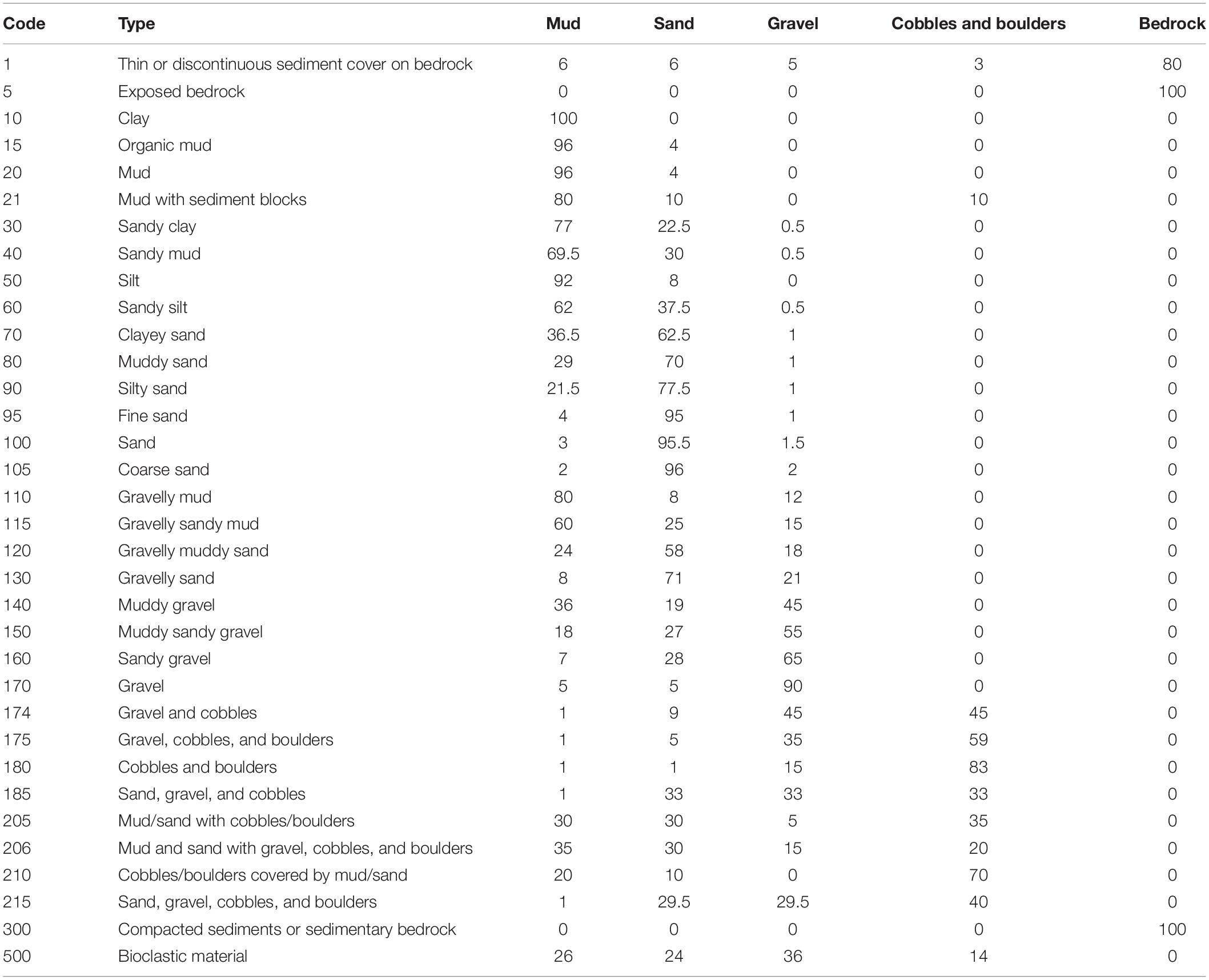
Table 1. Lookup table provided by the Geological Survey of Norway (NGU) for conversion of categorical sediment grain size classes to continuous sediment fractions.
Significant wave height and bottom wave exposure
The significant wave height is defined as the average height of the highest one-third of all waves. We applied the state-of-the-art, open-source wave model SWAN (Simulating WAves Nearshore1), developed at Delft University of Technology, Netherlands, to simulate the combined effect of wind-generated waves and swells in the coastal regions of the study area. The model grid applied had a 50 m × 50 m horizontal resolution using bathymetric data from the Norwegian Mapping Authority. The wave model was run in a non-stationary mode for approximately one winter month (January 2009) to cover most of the geographical variability in wave conditions. The atmospheric winds applied were provided every third hour from a 3 km × 3 km simulation using the Weather Research and Forecasting model (WRF, Skamarock et al., 2008). Wave spectra along the open boundaries on a 500 m × 500 m SWAN grid were provided every third hour by the Norwegian Meteorological Institute based on values from the Norwegian hindcast of wind and waves (NORA10) archive covering the Norwegian Sea (Reistad et al., 2011). Wave spectra from the SWAN-500 m model were then applied to force the SWAN-50 m model. The output from the highest resolution wave model (SWAN-50 m) consisted of time series of significant wave height and wave peak periods (wave lengths) valid every 3rd hour.
Waves are characterised with orbital motions dependent on water depth, wavelength and wave height. Similar to Rattray et al. (2015) we used linear wave theory to predict the maximum horizontal component of the wave orbital velocity on the sea bed for all grid points. Our formula, and then our proxy for Bottom wave exposure, writes:
where H is the significant wave height (m), T is the wave period (s), k is the wave number (k = 2∗π/L where L is the wavelength) and d is the water depth. Umax was calculated for every time step based on the wave model output. Due to strong collinearity between Significant wave height and Bottom wave exposure we decided to not use them in the same model. We used their 90-percentiles in the statistical analysis.
Bottom current speed
The three-dimensional, free-surface, hydrostatic, primitive equation ocean model ROMS (Haidvogel et al., 2008; Regional Ocean Modeling System2, Shchepetkin and McWilliams, 2005) was applied on a 160 m × 160 m grid covering the study area and adjacent regions to provide time series of current speed close to the sea floor. Applications using this model system have been documented in numerous manuscripts, e.g. Storesund et al. (2017) and Huserbråten et al. (2018). The 90-percentiles based on hourly output current speed from a 2-year long simulation were applied in the statistical analysis.
Stratification
Laminaria hyperborea dominates the shallow sublittoral down to 35 m (Kain and Jones, 1971), and for logistical reasons, no observations of kelp were made shallower than 3 m. Thus, for the purpose of the stratification, we applied a mask to the covariate rasters for pixels not matching the depth range of 3–35 m.
To stratify our study area, K-means clustering (Hartigan and Wong, 1979) was applied to the masked environmental covariate rasters using the kmeans function in the stats package in combination with a bespoke function. Choosing the optimal number of clusters in k-means is challenging. There exist approaches that are meant to provide guidance in this respect (Tibshirani et al., 2001). However, when using k-means clustering on large continuous raster datasets, there will not be any clear optimal solution where every point would seem to belong to a natural cluster. We, therefore, used the proportion of variance explained between clusters as a measure of optimality. This proportion is influenced by a range of factors, such as the extent of the survey area, the number of environmental covariates, and the variability of each covariate. Depending on these factors, a good solution can be expected to be found when 80 – 90% of the variance is explained between the clusters. Another criterion could be to set a threshold for what the increase in variance explained between clusters should be before stopping. Such a threshold could be 2 – 3%.
In the k-means classification analyses, we used bottom current speed, depth, significant wave height, and proportion of hard substrate. The raster of bottom wave exposure was not available at the time of planning the sampling strategy and was therefore not included in the k-means classification. The four covariates were standardised between 5 and 260 (due to potential inflation of the coefficient of variation values if means are small and close to zero, see below). This was done to give equal weight to the rasters in the analysis. Using a combination of the two criteria explained above, we settled on using 15 clusters. This solution had 81.5% of the variance explained between the clusters. Subsequently, a modal smoother function looking at 49 neighbouring pixels was applied, to reduce the resulting noise from the k-means clustering, as well as to show the more general trend of k-means classes across the study area. This representation of the k-means classification was polygonised and exported to a shapefile for later use in the implementation of the sampling strategy (Figure 3).
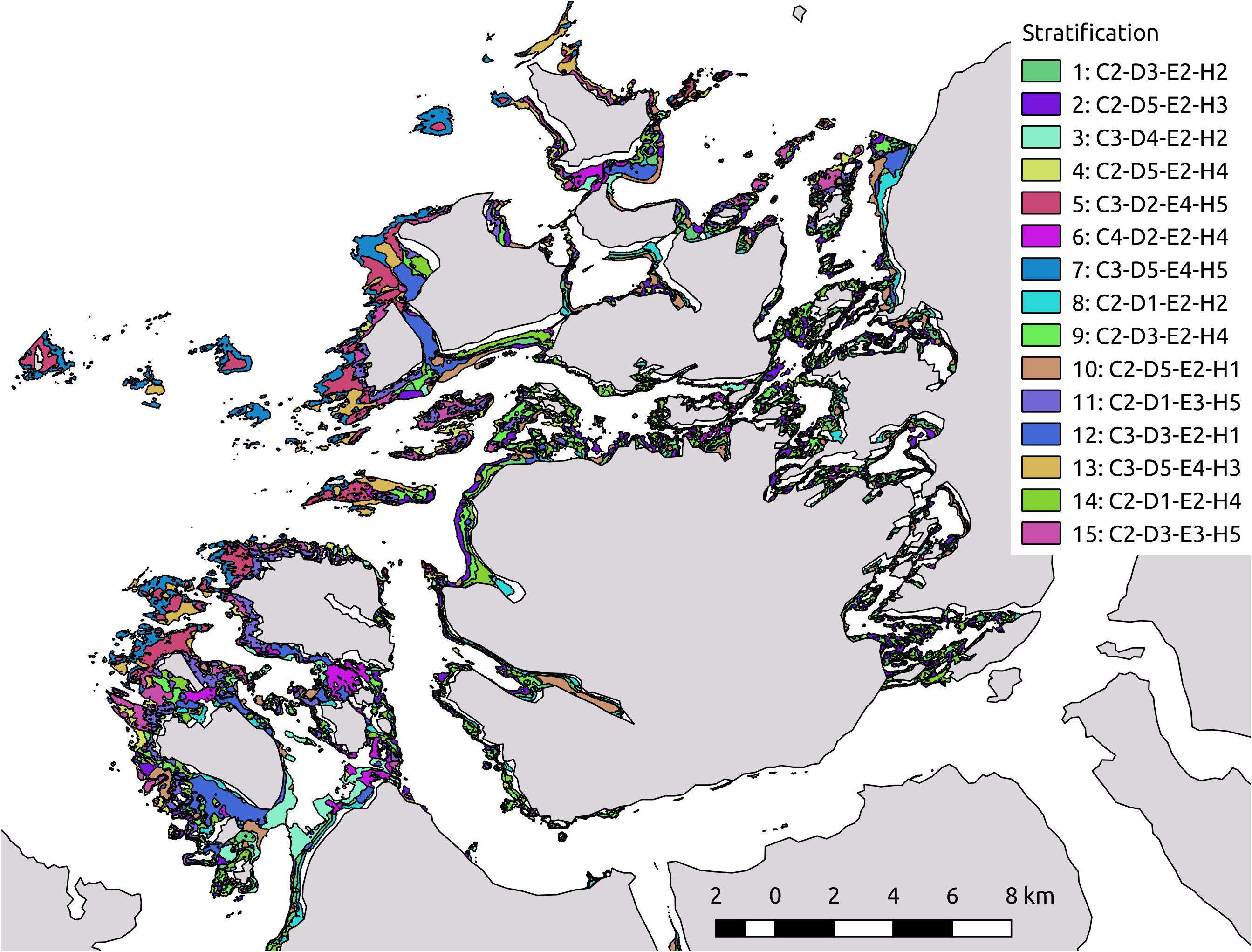
Figure 3. Map of stratification result from kmeans analysis. The stratification resulted in 15 strata that were used in the planning of sampling strategy. In an attempt to describe the environmental conditions of each stratum, the strata exhibited a code with combinations of four letters C (bottom Currents), D (Depth), E (wave Exposure/height), and H (proportion Hard substrate); and four numbers taking the values 1 (representing values between the 0 and 20 percentile for the environmental covariate in question), 2 (21 and 40 percentile), 3 (41 and 60 percentile), 4 (61 and 80 percentile), and 5 (81 and 100 percentile).
Allocation of Sampling Sites: GRTS
Generalised random tessellation strategy (GRTS, Stevens and Olsen, 2004) was used for spatial allocation of sampling sites within the study area. This strategy creates a collection of sample sites that are spatially balanced, i.e., more or less evenly distributed over the area of interest. When combined with a stratification of the study area, GRTS allocate sampling sites in a way that is in between what a conventional random, stratified sampling strategy and a regular grid (i.e., systematic) strategy would produce. This is more efficient in terms of capturing the spatial variability of a natural resource than a conventional random sample strategy (Stevens and Olsen, 2004).
Using the spsurvey package (Kincaid and Olsen, 2018) we applied a random stratified GRTS implementation with unequal inclusion probability. The 15 clusters from the k-means stratification were used as strata while the inclusion probability was calculated for each stratum based on their extent and their environmental variability. The extent of each stratum was calculated by summing the number of raster pixels within each stratum and then divide this sum by the total number of pixels in the study area. This gave us the proportional extent of each stratum. The environmental variability within each stratum was calculated by taking the coefficient of variation (CV = standard deviation/mean) for each covariate raster. We summed the CV for all the covariate rasters for each of the strata getting a total CV for each stratum, and this total was again summed to get a total CV for the whole dataset. Having this total CV we could calculate the proportional variability each stratum contributed to the whole. Both the proportions of extent and proportions of variability each summed to one.
Having these two proportions, we could calculate the inclusion probability for each stratum. This was done by giving the two proportions equal weight (50% each), which was simply achieved by summing the two proportions and divide the sum by two (Table 2). The importance of calculating this inclusion probability is to make sure that strata with larger extents get proportionally more samples allocated than strata with smaller extents and that strata with higher environmental variability get proportionally more samples allocated than strata with lower environmental variability.
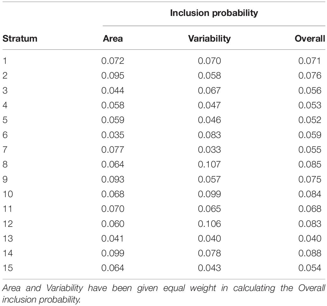
Table 2. Calculated inclusion probability per stratum.
Field Observations of Kelp Biomass
Observations of kelp biomass were made between depths of 3 and 35 m using a cable connected underwater drop camera (UVS 5080, 700 TVL), with a built-in depth sensor, sensitive to the nearest 0.1 m, deployed from a boat (Steen et al., 2016). A total of 154 sites were visited, but 9 had to be excluded based on them being marginally located outside the final study area, as defined by the area covered by the rasters of the predictors. An independent dataset of 80 sites surveyed across the study area for the Norwegian Programme for Mapping of Marine Habitats was analysed for kelp biomass and used for model evaluation.
The field work was carried out between April and June 2017. At each site, the camera was lowered onto the seabed to observe the kelp coverage, density and height (Steen et al., 2016). Kelp coverage was estimated as percentage kelp coverage of the seabed, from camera views above the kelp canopy layer. The average height of L. hyperborea kelp plants was measured as the depth difference, read from the depth sensor measurements when the camera was moved vertically between the seabed and the top of the kelp fronds. Density estimates were obtained by counting the number of L. hyperborea canopy plants per m2 (fitted by eye) from horizontal camera views beneath the kelp canopy lamina layer. If kelp plant numbers were high and frond height low, density was classified in groups (e.g. 10, 12.5, 15, 20 kelp plants per m–2). The height and density estimates were later used to estimate the biomass of L. hyperborea [kg FW/m2] by multiplying density [in kelp plants per m2] with fresh weight [in kg per kelp plant]. Kelp plant weight (in kg) were related to kelp plant height (in m) by the conversion formula:
This formula has a correlation of 0.88 obtained from correlating fresh weight and height measurements of kelp plants collected by dredging (Steen et al., 2016).
In order to verify the accuracy of this method for estimating biomass of L. hyperborea, divers revisited a selection of the same sites that had been observed by camera. A total of 11 of the 145 sites were randomly selected within a stratification based on observed biomass, significant wave height and depth. At each of these eleven sites, all plants within 1 m2 were collected and subsequently counted, measured, and weighed. The biomass estimated from the two methods were found to be highly correlated (correlation of 0.77).
Statistical Analyses
Generalised additive models (GAMs, Hastie and Tibshirani, 1990) were applied to model the relationship between the biomass of Laminaria hyperborea and the environmental predictors. The biomass of L. hyperborea was considered to follow a mixed compound Poisson–gamma distribution which has positive mass at zero but otherwise is continuous. This formulation belongs to what is known as the Tweedie family of distributions (Tweedie, 1984; Jorgensen, 1987; Foster and Bravington, 2013) and can handle the combination of a large number of zero observations and strictly positive biomass observations well. With biomass of L. hyperborea as the response variable, the selection of the GAM smoothing predictors was carried out with MGCV package (Wood, 2011) in the R statistical software (R Core Team, 2018). In each fitted model, a double penalty is applied to the penalised regression solved by MGCV, which allows variables to be solved out of the model entirely (Marra and Wood, 2011), being more robust to identify important features. The degree of smoothing was chosen based on the observed data and the restricted maximum likelihood (REML) with the maximum degrees of freedom (measured as the number of knots, k) allowed to the smoothing functions limited to 5 to avoid over-fitting.
The following main-effects-only model was initially fitted:
where i denotes observation sites, and a backward model selection was carried out to find the most parsimonious model formulation. We did not include any first-order interactions in our models to allow for easier interpretability of the models. Model validation plots (e.g., residuals versus fitted values, QQ-plots and residuals versus the original explanatory variables) were used to explore for model misspecification. Residuals were also checked for spatial autocorrelation by visually inspecting for patterns in the 2D space, as well as with semi-variogram plots. The output of the final selected GAMs is presented as plots of the best-fitting smooths.
All resulting statistical models were used to predict to the whole study area. For this exercise, all the predictors were aggregated or disaggregated to a common resolution resulting in a spatial biomass model of L. hyperborea with 20 m resolution. Subsequently, the model evaluation was carried out using the independently collected dataset from the same study area and correlating it with the predicted biomass values from the different statistical models.
Results
An environmental covariate space analysis is done by plotting all potential combinations of pixel values for two or more covariates against each other and then plotting the field observations on top. This was done between depth and the covariates used to plan the sampling strategy and used in the GAM modelling. By visually inspecting these plots (Figure 4), we can see that the 145 observations to a large degree cover the whole environmental covariate space.
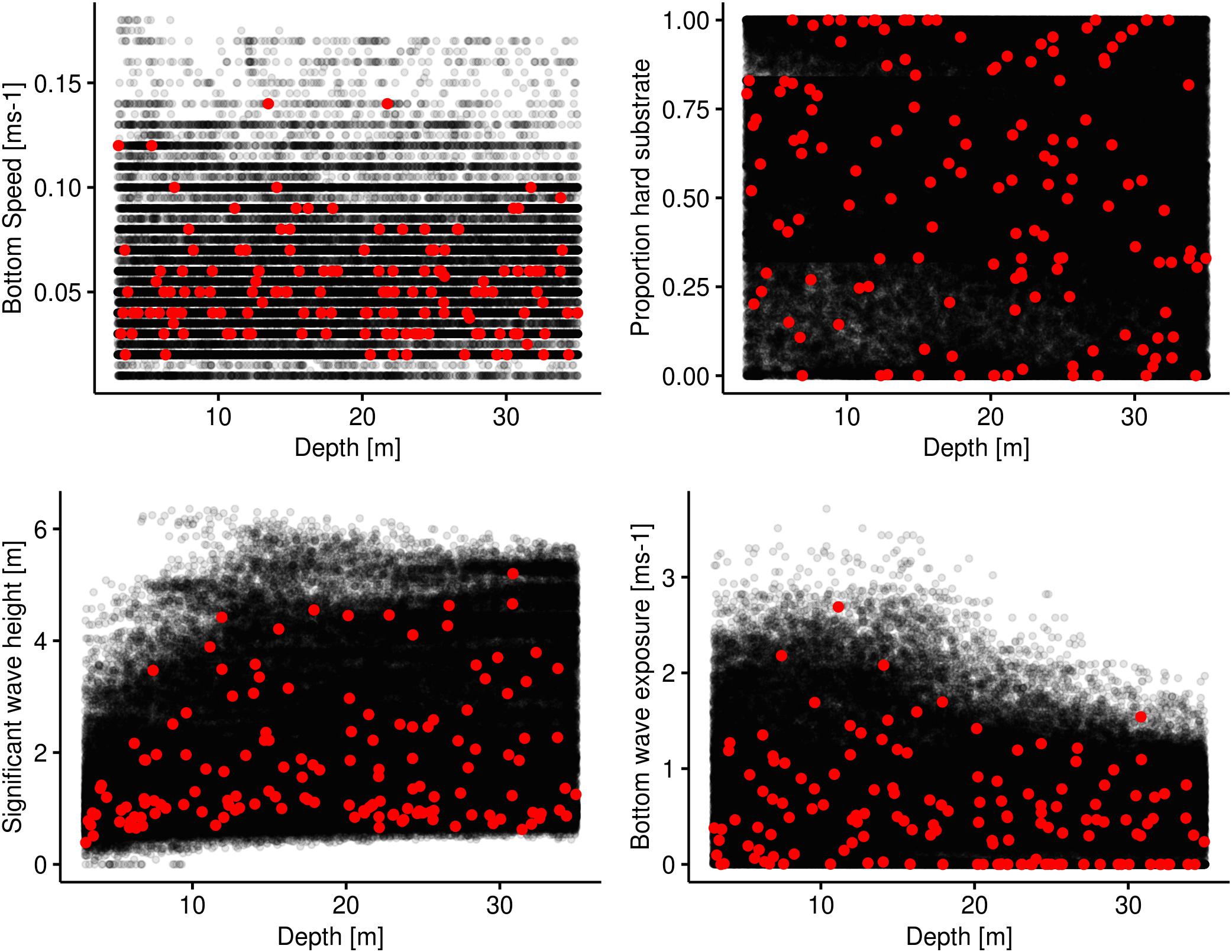
Figure 4. Environmental covariate space plots. Depth is used as the base covariate for which each of the remaining covariates are plotted against. The black dots represent the realised environmental combinations in the study area of the two covariates in question. The red dots represent the values at the sampled sites. The black dots are plotted with a transparency of 0.1.
We fitted a total of three GAM models that were assessed based on their REML and AIC values. An additional fourth model was fitted in order to test whether the bottom wave exposure covariate provided a model improvement over the conventional significant wave height covariate. The model containing depth, proportion hard substrate, and bottom wave exposure had the lowest REML and AIC values, although only marginally lower than the model containing bottom current speed in addition to the three aforementioned covariates. These two models explained about 83% of the deviance. A third model containing only depth and bottom wave exposure led to a large increase in both REML and AIC values as well as a decrease in deviance explained (Table 3).
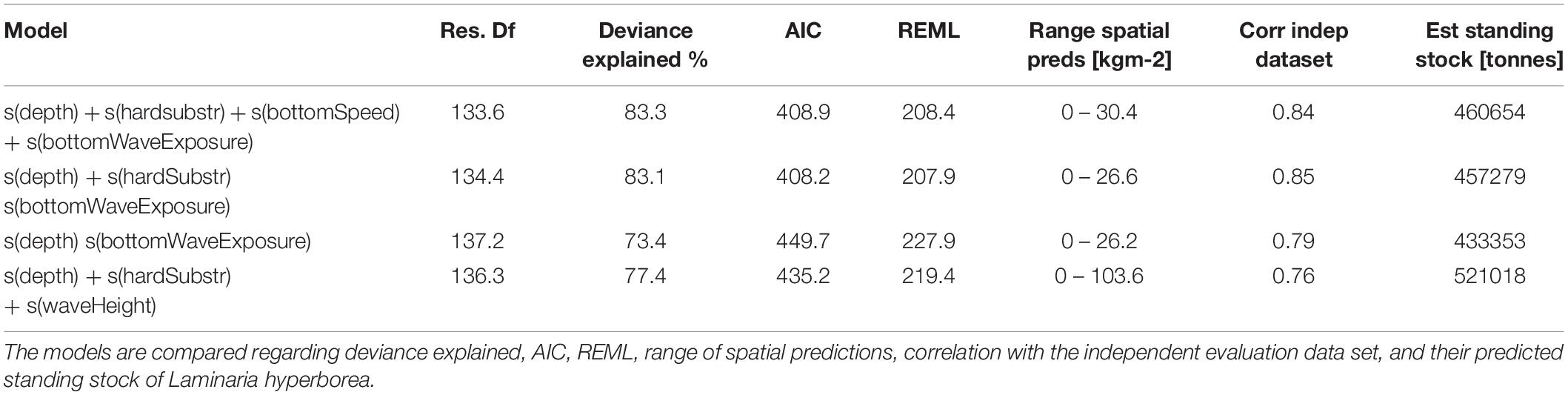
Table 3. Statistical summary of fitted GAM models and their predictive performance.
As we removed covariates in the models, bottom wave exposure became increasingly more important. The response curve for this covariate, based on the model with the lowest REML and AIC values, shows that bottom wave exposure below 0.3 ms-1 has a negative impact on the biomass of L. hyperborea. Between 0.3 ms-1s and 0.8 ms-1 bottom wave exposure has an increasingly positive impact on the biomass. For values above 0.8 ms-1, the impact of bottom wave exposure reaches a plateau but continues to have a positive impact on biomass, even in very exposed areas (Figure 5). It is important to note here that there are very few observations with bottom wave exposure values above 1.5 ms-1. This is a consequence of this covariate not being available when the sampling strategy was planned. Depth, being a proxy for light primarily, seemed to be the second most important covariate in explaining the variance in kelp biomass. The response curve of depth has an optimum at around 10 m. Below 20 m depth, depth starts to have an increasingly detrimental effect on the biomass. For proportion hard substrate, the response curve suggests there is a threshold around a proportion of hard substrate of 0.5 in which below this value biomass is decreasing and above biomass is increasing.
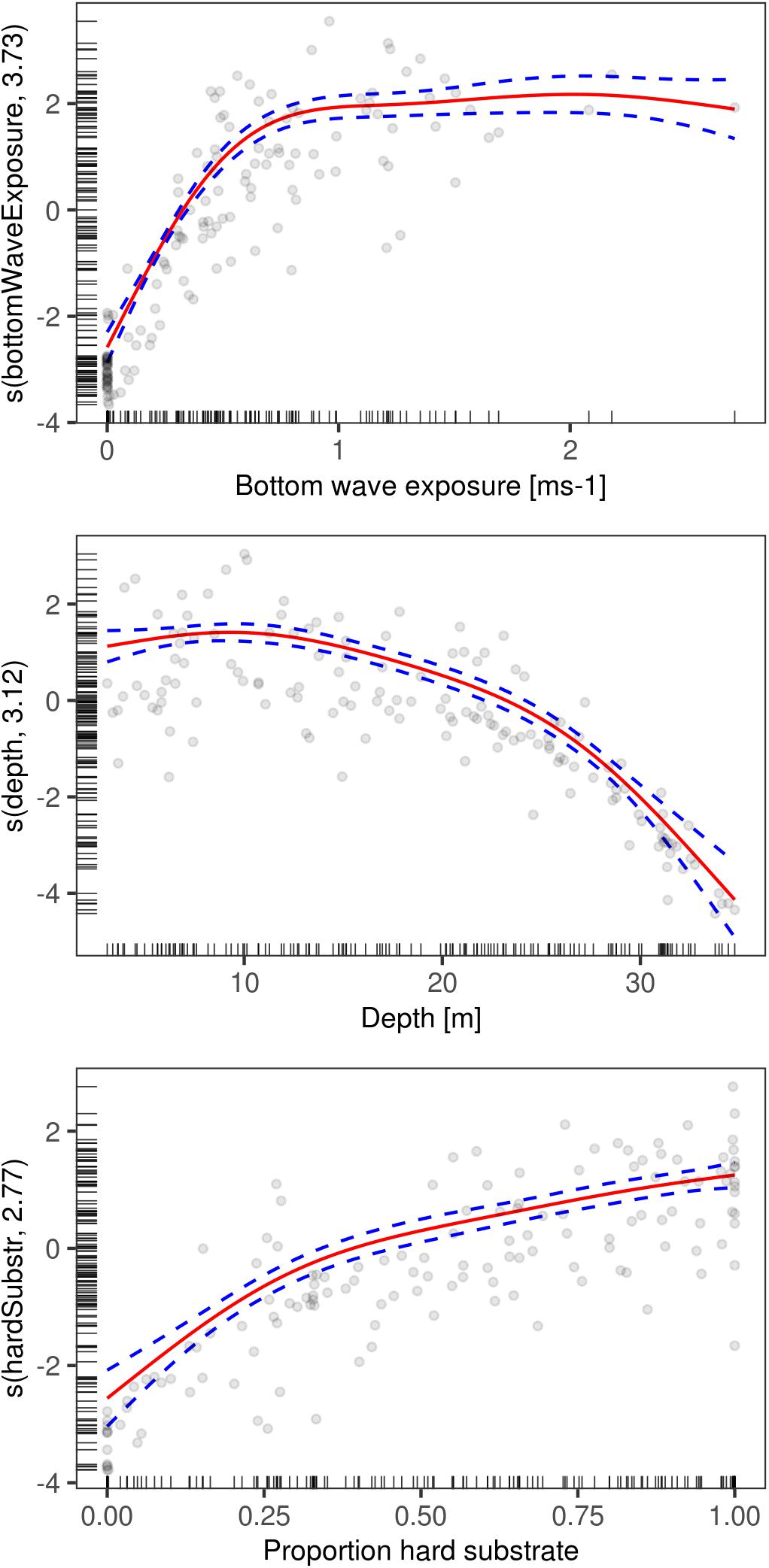
Figure 5. GAM response curves of the biomass of Laminaria hyperborea for the model containing the predictors bottom wave exposure, depth, and proportion hard substrate. The y-axis indicates the relative influence of each predictor on the biomass. The fitted line is in red with blue lines representing 1 SE. Grey, hollow circles represent observation points.
We decided to perform spatial predictions based on all models. This allowed us to later compare their spatial predictions to our independent evaluation dataset. The range of the values of spatial predictions of biomass for L. hyperborea had minimum values at zero whereas the maximum values ranged between 26.6 (model with depth, proportion hard substrate, and bottom wave exposure) and 30.4 (model with all four covariates) kgm-2 (Table 3). The spatial predictions of all three models were highly correlated with our independent evaluation dataset with Pearson’s correlation coefficient R ranging between 0.79 and 0.85 (Table 3). We consider the model containing depth, proportion hard substrate, and bottom wave exposure the best, balancing model complexity and predictive power very well (see Figure 6 for its spatial prediction and Figure 7 for its correlation with the independent evaluation dataset). It is important to note though, that the three main models differed very little in predictive performance. The total predicted biomass of L. hyperborea for the selected model in the study area (∼1,150 km2) was 457,000 tonnes (Table 3).
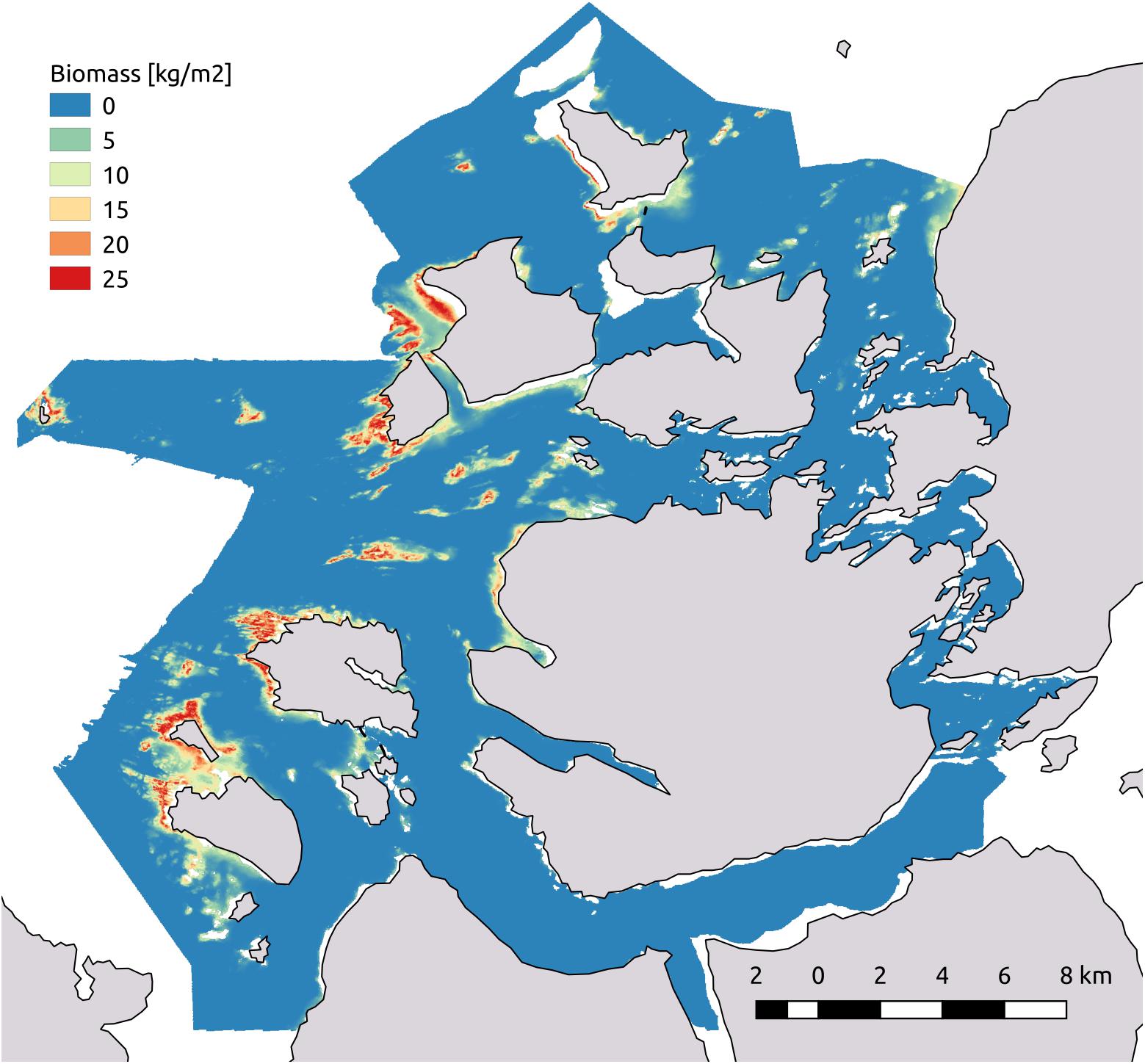
Figure 6. Map of the spatial predictions of biomass of Laminaria hyperborea in kgm-2. Predictions are based on the model containing the predictors bottom wave exposure, depth, and proportion hard substrate.
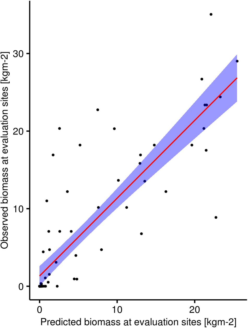
Figure 7. Plot showing the correlation between observed biomass of Laminaria hyperborea in the field at sites in the independent evaluation dataset and the predicted biomass at these sites by the model containing the predictors bottom wave exposure, depth, and proportion hard substrate. Red line is the line of best fit and the shaded blue area represent 95% confidence intervals.
The fourth model was identical to the model we considered the best, except that the bottom wave exposure was exchanged with the significant wave height (i.e., wave exposure on the sea surface). This model had a large increase in both REML and AIC values and a reduction in deviance explained (Table 3). In addition, this model predicted a much higher maximum value for biomass (103.6 kgm-2) and it also predicted a much higher standing stock, 521,000 tonnes. Even though it had a high correlation coefficient (R = 0.76) with the independent evaluation data set, it clearly often overpredicts biomass.
Discussion
By use of explicit measures of biomass (in kg FWm-2) of Laminaria hyperborea and statistical modelling, we were able to predict direct and accurate estimates of its spatial distribution and standing stock within our study area. We achieved a very good correlation between our spatial predictions of kelp biomass and an independent evaluation dataset. Having such an independent evaluation dataset is a more robust way to really test the performance of a statistical model and the accuracy of spatial predictions. Furthermore, we argue that through obtaining such a good correlation between predicted biomass and the evaluation dataset, our results clearly demonstrate the importance of a well-thought sampling strategy that optimises the coverage of the environmental covariate space as well as the inclusion of covariates that have a direct effect on the response. Our modelling approach also allows for an accurate quantification of the uncertainty in the final biomass estimations. Traditionally, uncertainty in model performance is mostly assessed by dividing a data set in a training and a test data set or by cross-validation. These traditional methods have only limited predictive power because they perform accurately for the provided dataset but usually provide poor predictions when new datasets are fed into the models. The commonly used covariate for kelp distribution modelling, wave exposure at the sea surface (Bajjouk et al., 2015; i.e., wave exposure at the sea surface; Bekkby et al., 2009; Gorman et al., 2012; Gregr et al., 2018), did not perform as well as bottom wave exposure in predicting the spatial distribution of L. hyperborea in our study. Interestingly, the model containing significant wave height (i.e., wave exposure at the sea surface) appeared to perform quite well in the statistical modelling. Only when predicting to new data and when comparing those predictions with the independent evaluation dataset did it become apparent that this fourth model underperforms substantially compared to the same model but with bottom wave exposure substituting wave exposure at sea surface. Hence, an independent evaluation data set is crucial in order to properly address the variance-bias trade-off in a model (Friedman et al., 2001); to identify the appropriate model complexity (Gregr et al., 2018); and to assess the accuracy and uncertainty in model predictions.
Wave exposure, either in the form of wind fetch or significant wave height, is used as a covariate in all published kelp models. However, kelp is affected by the wave energy at or near the sea floor. The wave energy is thus interacting with depth in a manner that in general reduces it with increasing depth. The importance of this interaction has also been recognised by other researchers (Bekkby et al., 2008; Bajjouk et al., 2015). Without its inclusion, our statistical model of kelp biomass faced problems in deep areas where the surface wave energy (i.e., significant wave height) is too high (i.e., not enough light available) for the kelp to thrive.
However, a simple statistical interaction between those two covariates was insufficient to describe their joint effect on kelp biomass. The interaction between the two was better explained by the implementation of a new covariate (i.e., bottom wave exposure) based on linear wave theory, similar to the methods applied in Rattray et al. (2015). Rattray et al. (2015) presented a method for extending wave exposure from a surface covariate to a seabed covariate. They used estimations of wave-induced orbital velocities at the seabed from wave models as a surrogate for wave exposure. For instance, at equal depths, waves with approximately similar significant wave heights will differ with respect to exposure on the seabed if the wavelengths (wave periods) are different. Long waves, typically induced by offshore swells, will have a larger impact on the seabed than shorter waves, often associated with wind-induced waves. The covariate representing the maximum wave-induced orbital velocity on the seabed, explained in Rattray et al. (2015) as a function of wave height, wavelength, and ocean depth, became a crucial covariate in our model.
In addition to bottom wave exposure, our results show there are important relationships between the biomass of L. hyperborea and the predictors of depth and the proportion hard substrate. While depth is often used in similar studies (Bekkby et al., 2009; Young et al., 2015; Gregr et al., 2018), both proportion hard substrate and bottom wave exposure are less often used because they are rarely available. The two latter covariates are of particular interest because they represent more direct (i.e., proximate) effects on kelp biomass. Often, researchers do not have access to processes directly influencing biological responses, and often use proxies that to a varying degree are correlated with the covariates that directly explain this variance.
As with altitude in terrestrial studies, bathymetry or depth is often used as a covariate in marine studies. Both altitude and ocean depth are often statistically important covariates since they act as proxies for many unmeasured proximate factors. As such, depth can act as a proxy for temperature, salinity, nutrient and particle concentrations, change in wave energy, and light, with light being the most important as light is the energy source for kelp growth (Gattuso et al., 2006).
In our study, the depth covariate primarily acts as a proxy for light and wave energy, which both decrease with increasing depth. Regarding depth as a proxy for light in our study area, light conditions are assumed to exhibit little spatial variation given that the study area is far out in the archipelago with clear water and there are no major rivers or other factors that are expected to introduce significant variability in water transparency, hence light conditions. Other studies modelling the spatial distribution of kelp (Bekkby et al., 2009; Gorman et al., 2012; Young et al., 2015) also report the importance of depth, often being the most influential covariate. In this study we have high-resolution bathymetry at our disposal, however, due to military restrictions, this is not the case in most areas along the Norwegian coast where 50 m resolution is the norm.
Kelp species such as L. hyperborea require hard substrate to anchor their holdfasts and develop (Kain and Jones, 1971). Given the statistical importance of proportion of hard substrate, our study and the one by Young et al. (2015), underpins the value of accurate substrate maps when modelling the spatial distribution of kelp forests. A good model of hard substrate can explain as much as or more of the variance as depth can do (Young et al., 2015; Gregr et al., 2018). However, most studies do not have access to a raster of hard substrate and need to use terrain variables such as slope (Bekkby et al., 2009; Gorman et al., 2012; Rattray et al., 2015; Gregr et al., 2018), curvature (Bekkby et al., 2009; Rattray et al., 2015), or rugosity (Rattray et al., 2015) as proxies instead. While such proxies to a varying degree seem to pick up some of the variance explained by the hard substrate, future studies should strive to include hard substrate directly.
There is an increasing need for reliable predictions of the spatial distribution of kelp biomass. Recently, the potential of kelp forests in capturing and storing carbon from the atmosphere has been recognised (Krause-Jensen and Duarte, 2016). Most of the kelp production is not consumed inside the kelp forest but exported. An unknown part is transported to deep water where it is fuelling communities or buried and thereby removed from the quick carbon cycle. The significance of this role is more or less unknown and has therefore been referred to as “the elephant in the blue carbon room” (Krause-Jensen and Duarte, 2016). To increase the understanding of the role of kelp forests in the larger coastal ecosystem, data on biomass, production, spatial distribution, transport processes, and consumption are all of principal importance. Our model can be applied to larger areas and is a step forward filling gaps with regard to biomass and its spatial distribution.
Kelp is harvested by humans and some 160,000 tonnes are being harvested in Norway annually. The importance of kelp forests as feeding and nursery areas for coastal fish and seabirds and lack of quantitative knowledge about resource sizes generate conflicts between different stakeholders. To ensure an improved harvesting regime it will be important to quantify the available resources and address how much of the standing stock is harvested in different areas. A spatial biomass model, like the one developed in this study, in combination with good harvest data is crucial to address this question.
This study provides a snapshot in time of the standing stock of L. hyperborea in the study area. The temporal variability of the spatial distribution and its standing stock remain largely unknown. The presented modelling framework can be used both on a regional and national scale, although data available at these scales have a lower quality (i.e. lower resolution) compared to the data available in this study. Future biomass assessments should strive to apply more efficient remote sensing techniques (Bell et al., 2015; Nijland et al., 2019), although these techniques will not work properly for L. hyperborea that often form canopies way below the surface and out of reach for those sensors. Such techniques, however, are more readily replicated in time and have the potential to provide crucial insights into the temporal dynamics of kelp forest biomass over larger areas.
Data Availability Statement
The datasets for this study are available upon request.
Author Contributions
TS planned the fieldwork, did the statistical analysis with NN, and led the writing with contributions from all co-authors. HS led the fieldwork and conceived the project together with FM and KN. JA and BF prepared the oceanographic covariates. SE prepared the sediment map.
Funding
The research was partially financed by FMC Biopolymer (Dupont).
Conflict of Interest
The authors declare that the research was conducted in the absence of any commercial or financial relationships that could be construed as a potential conflict of interest.
Acknowledgments
This project was performed together with and partially financed by FMC Biopolymer (Dupont) as a cooperative partner. Special thanks to Torjan Bodvin for initiating this project and to Lene Christensen for invaluable assistance in the field. We also want to thank the three reviewers for commenting on and helping us improve the manuscript.
Footnotes
References
Bajjouk, T., Rochette, S., Laurans, M., Ehrhold, A., Hamdi, A., and Le Niliot, P. (2015). Multi-approach mapping to help spatial planning and management of the kelp species L. digitata and L. hyperborea: case study of the Molène Archipelago, Brittany. J. Sea Res. 100, 2–21. doi: 10.1016/j.seares.2015.04.004
Bekkby, T., Isachsen, P. E., Isæus, M., and Bakkestuen, V. (2008). GIS modeling of wave exposure at the seabed: a depth-attenuated wave exposure model. Mar. Geod. 31, 117–127. doi: 10.1080/01490410802053674
Bekkby, T., Rinde, E., Erikstad, L., and Bakkestuen, V. (2009). Spatial predictive distribution modelling of the kelp species Laminaria hyperborea. ICES J. Mar. Sci. 66, 2106–2115. doi: 10.1093/icesjms/fsp195
Bell, T. W., Cavanaugh, K. C., and Siegel, D. A. (2015). Remote monitoring of giant kelp biomass and physiological condition: an evaluation of the potential for the hyperspectral infrared imager (HyspIRI) mission. Remote Sens. Environ. 167, 218–228. doi: 10.1016/j.rse.2015.05.003
Bjørge, A., Thompson, D., Hammond, P., Fedak, M., Bryant, E., Aarefjord, H., et al. (1995). “Habitat use and diving behaviour of harbour seals in a coastal archipelago in Norway,” in Developments in Marine Biology, eds A. S. Blix, L. Walløe, and Ø Ulltang, (Amsterdam: Elsevier), 211–223. doi: 10.1016/s0163-6995(06)80025-9
Bøe, R., Dolan, M., Thorsnes, T., Lepland, A., Olsen, H., Totland, O., et al. (2010). Standard for Geological Seabed Mapping Offshore. NGU Report 2010.033. Trondheim: Geological Survey of Norway.
Cavanaugh, K. C., Siegel, D. A., Reed, D. C., and Dennison, P. E. (2011). Environmental controls of giant-kelp biomass in the Santa Barbara Channel California. Mar. Ecol. Prog. Ser. 429, 1–17. doi: 10.3354/meps09141
Elith, J., and Leathwick, J. (2007). Predicting species distributions from museum and herbarium records using multiresponse models fitted with multivariate adaptive regression splines. Divers. Distrib. 13, 265–275. doi: 10.1111/j.1472-4642.2007.00340.x
Elvenes, S., Bøe, R., Lepland, A., and Dolan, M. (2019). Seabed sediments of Søre Sunnmøre Norway. J. Maps 15, 686–696. doi: 10.1080/17445647.2019.1659865
Folk, R. L. (1954). The distinction between grain size and mineral composition in sedimentary-rock nomenclature. J. Geol. 62, 344–359. doi: 10.1086/626171
Foster, S. D., and Bravington, M. V. (2013). A poisson–gamma model for analysis of ecological non-negative continuous data. Environ. Ecol. Stat. 20, 533–552. doi: 10.1007/s10651-012-0233-0
Friedman, J., Hastie, T., and Tibshirani, R. (2001). The Elements of Statistical Learning. New York, NY: Springer.
Gattuso, J.-P., Gentili, B., Duarte, C. M., Kleypas, J. A., Middelburg, J. J., and Antoine, D. (2006). Light availability in the coastal ocean: impact on the distribution of benthic photosynthetic organisms and their contribution to primary production. Biogeosciences 3, 489–513. doi: 10.5194/bg-3-489-2006
Gorman, D., Bajjouk, T., Populus, J., Vasquez, M., and Ehrhold, A. (2012). Modeling kelp forest distribution and biomass along temperate rocky coastlines. Mar. Biol. 160, 309–325. doi: 10.1007/s00227-012-2089-0
Gräler, B., Pebesma, E., and Heuvelink, G. (2016). Spatio-temporal interpolation using gstat. R. J. 8, 204–218.
Gregr, E. J., Palacios, D. M., Thompson, A., and Chan, K. M. A. (2018). Why less complexity produces better forecasts: an independent data evaluation of kelp habitat models. Ecography 43:1223.
Guisan, A., and Zimmermann, N. E. (2000). Predictive habitat distribution models in ecology. Ecol. Modell. 135, 147–186. doi: 10.1016/s0304-3800(00)00354-9
Haidvogel, D. B., Arango, H., Budgell, W. P., Cornuelle, B. D., Curchitser, E., Di Lorenzo, E., et al. (2008). Ocean forecasting in terrain-following coordinates: formulation and skill assessment of the regional ocean modeling system. J. Comput. Phys. 227, 3595–3624. doi: 10.1016/j.jcp.2007.06.016
Hartigan, J. A., and Wong, M. A. (1979). Algorithm AS 136: A K-means clustering algorithm. J. R. Stat. Soc. Ser. C Appl. Stat. 28, 100–108.
Hijmans, R. J. (2018). Raster: Geographic Data Analysis and Modeling. Available at: https://CRAN.R-project.org/package=raster
Huserbråten, M. B. O., Moland, E., and Albretsen, J. (2018). Cod at drift in the North Sea. Prog. Oceanogr. 167, 116–124. doi: 10.1016/j.pocean.2018.07.005
Jorgensen, B. (1987). Exponential dispersion models. J. R. Stat. Soc. Series B Stat. Methodol. 49, 127–162.
Kain, J. M., and Jones, N. S. (1971). The biology of Laminaria hyperborea. VI. some norwegian populations. J. Mar. Biol. Assoc. U. K. 51, 387–408. doi: 10.1017/s0025315400031866
Kincaid, T. M., and Olsen, A. R. (2018). Spsurvey: Spatial Survey Design and Analysis. R Package Version 3.4.
Krause-Jensen, D., and Duarte, C. M. (2016). Substantial role of macroalgae in marine carbon sequestration. Nat. Geosci. 9, 737–742. doi: 10.1007/s13280-016-0849-7
Lorentsen, S.-H., Sjøtun, K., and Grémillet, D. (2010). Multi-trophic consequences of kelp harvest. Biol. Conserv. 143, 2054–2062. doi: 10.1016/j.biocon.2010.05.013
Marra, G., and Wood, S. N. (2011). Practical variable selection for generalized additive models. Comput. Stat. Data Anal. 55, 2372–2387. doi: 10.1016/j.csda.2011.02.004
Nijland, W., Reshitnyk, L., and Rubidge, E. (2019). Satellite remote sensing of canopy-forming kelp on a complex coastline: a novel procedure using the Landsat image archive. Remote Sens. Environ. 220, 41–50. doi: 10.1016/j.rse.2018.10.032
Norderhaug, K. M., and Christie, H. (2011). Secondary production in a Laminaria hyperborea kelp forest and variation according to wave exposure. Estuar. Coast. Shelf Sci. 95, 135–144. doi: 10.1016/j.ecss.2011.08.028
Norderhaug, K. M., Christie, H., Fosså, J. H., and Fredriksen, S. (2005). Fish-macrofauna interactions in a kelp (Laminaria hyperborea) forest. J. Mar. Biol. Assoc. U. K. 85:1279. doi: 10.1007/BF00330016
Norderhaug, K. M., Fredriksen, S., and Nygaard, K. (2003). Trophic importance of Laminaria hyperborea to kelp forest consumers and the importance of bacterial degradation to food quality. Mar. Ecol. Prog. Ser. 255, 135–144. doi: 10.3354/meps255135
Pebesma, E. J. (2004). Multivariable geostatistics in S: the gstat package. Comput. Geosci. 30, 683–691. doi: 10.1016/j.cageo.2004.03.012
Rattray, A., Ierodiaconou, D., and Womersley, T. (2015). Wave exposure as a predictor of benthic habitat distribution on high energy temperate reefs. Front. Mar. Sci. 2:161. doi: 10.3389/fmars.2015.00008
Raybaud, V., Beaugrand, G., Goberville, E., Delebecq, G., Destombe, C., Valero, M., et al. (2013). Decline in kelp in west europe and climate. PLoS One 8:e66044. doi: 10.1371/journal.pone.0066044
Reistad, M., Breivik, O., Haakenstad, H., Aarnes, O. J., Furevik, B. R., and Bidlot, J.-R. (2011). A high-resolution hindcast of wind and waves for the North Sea, the Norwegian Sea, and the Barents Sea. J. Geophys. Res. C Oceans 116:C05019.
Shchepetkin, A. F., and McWilliams, J. C. (2005). The regional oceanic modeling system (ROMS): a split-explicit, free-surface, topography-following-coordinate oceanic model. Ocean Model. 9, 347–404. doi: 10.1016/j.ocemod.2004.08.002
Sjøtun, K., Fredriksen, S., Lein, T. E., Rueness, J., and Sivertsen, K. (1993). “Population studies of Laminaria hyperborea from its northern range of distribution in Norway,” in Proceedings of the Fourteenth International Seaweed Symposium, Berlin, 215–221. doi: 10.1007/bf00049022
Skamarock, W. C., Klemp, J. B., Dudhia, J., Gill, D. O., Barker, D. M., Duda, M. G., et al. (2008). A Description of the Advanced Research WRF Version 3. Boulder, CO: NCAR.
Steen, H., Moy, F. E., Bodvin, T., and Husa, V. (2016). Regrowth after kelp harvesting in Nord-Trøndelag Norway. ICES J. Mar. Sci. 73, 2708–2720. doi: 10.1093/icesjms/fsw130
Steneck, R. S., Graham, M. H., Bourque, B. J., Corbett, D., Erlandson, J. M., Estes, J. A., et al. (2002). Kelp forest ecosystems: biodiversity, stability, resilience and future. Environ. Conserv. 29, 436–459. doi: 10.1017/s0376892902000322
Stevens, D. L. Jr., and Olsen, A. R. (2004). Spatially balanced sampling of natural resources. J. Am. Stat. Assoc. 99, 262–278. doi: 10.1198/016214504000000250
Storesund, J. E., Sandaa, R.-A., Thingstad, T. F., Asplin, L., Albretsen, J., and Erga, S. R. (2017). Linking bacterial community structure to advection and environmental impact along a coast-fjord gradient of the Sognefjord, western Norway. Prog. Oceanogr. 159, 13–30. doi: 10.1016/j.pocean.2017.09.002
Teagle, H., Hawkins, S. J., Moore, P. J., and Smale, D. A. (2017). The role of kelp species as biogenic habitat formers in coastal marine ecosystems. J. Exp. Mar. Bio. Ecol. 492, 81–98. doi: 10.1016/j.jembe.2017.01.017
Tibshirani, R., Walther, G., and Hastie, T. (2001). Estimating the number of clusters in a data set via the gap statistic. J. R. Statist. Soc. 63, 411–423. doi: 10.1111/1467-9868.00293
Tweedie, M. C. K. (1984). “An index which distinguishes between some important exponential families,” in Statistics: Applications and New Directions: Proceedings of the Indian Statistical Institute Golden Jubilee International Conference, eds J. K. Ghosh and J. Roy, (Calcutta: Indian Statistical Institute), 579–604.
Vilalta-Navas, A., Beas-Luna, R., Calderon-Aguilera, L. E., Ladah, L., Micheli, F., Christensen, V., et al. (2018). A mass-balanced food web model for a kelp forest ecosystem near its southern distributional limit in the northern hemisphere. Food Webs 17:e00091. doi: 10.1016/j.fooweb.2018.e00091
Wood, S. N. (2011). Fast stable restricted maximum likelihood and marginal likelihood estimation of semiparametric generalized linear models. J. R. Statist. Soc. 73, 3–36. doi: 10.1111/j.1467-9868.2010.00749.x
Keywords: biomass modelling, bottom wave exposure, independent evaluation, Laminaria hyperborea, management, sampling strategy, species distribution modelling
Citation: van Son TC, Nikolioudakis N, Steen H, Albretsen J, Furevik BR, Elvenes S, Moy F and Norderhaug KM (2020) Achieving Reliable Estimates of the Spatial Distribution of Kelp Biomass. Front. Mar. Sci. 7:107. doi: 10.3389/fmars.2020.00107
Received: 05 April 2019; Accepted: 10 February 2020;
Published: 21 February 2020.
Edited by:
Alberto Basset, University of Salento, ItalyReviewed by:
Rodrigo Riera, Catholic University of the Most Holy Conception, ChileDominique Davoult, Sorbonne Universités, France
Inka Bartsch, Alfred Wegener Institute for Polar and Marine Research, Germany
Copyright © 2020 van Son, Nikolioudakis, Steen, Albretsen, Furevik, Elvenes, Moy and Norderhaug. This is an open-access article distributed under the terms of the Creative Commons Attribution License (CC BY). The use, distribution or reproduction in other forums is permitted, provided the original author(s) and the copyright owner(s) are credited and that the original publication in this journal is cited, in accordance with accepted academic practice. No use, distribution or reproduction is permitted which does not comply with these terms.
*Correspondence: Thijs Christiaan van Son, dGhpanMudmFuc29uQGhpLm5v