Satellite-Driven Estimates of Water Mass Formation and Their Spatio-Temporal Evolution

We derive water mass transformation and formation rates using satellite-derived datasets of salinity, temperature and fluxes of heat and freshwater over the North Atlantic, North Pacific and Southern Ocean. The formation rates are expressed in three coordinate systems: (1) density, (2) temperature-salinity and (3) latitude-longitude. In the North Atlantic and North Pacific, peak formation occurs south of the western boundary current extensions during the winter months of the study period. In the Southern Ocean, wintertime peak formation occurs just north of the sub-Antarctic Front. The satellite-derived water mass properties and formation areas agree well with previous estimates from literature. The location of peak Mode Water formation varies slightly with time in all coordinate systems. We assess seasonal and inter-annual variability in all three basins from 2012 to 2014. We assess the impact of satellite uncertainties on final estimates of formation rates and areas with Monte-Carlo simulations. The simulations provide insights on the associated uncertainty of formation estimates. They also provide information on the geographic spread of the water mass formation area subject to the satellite errors. We find that the total uncertainty is dominated by the uncertainty in the sea surface salinity dataset. This stresses the need for frequent and increasingly accurate sea surface salinity data for reliable estimates of water mass formation rates and areas. Our study highlights the feasibility of providing satellite-based estimates of water mass formation rates and areas. The good spatio-temporal coverage of satellite data further adds to the utility of the approach.

1. Introduction

Sea Surface Salinity (SSS) and Sea Surface Temperature (SST) are mostly set by heat and freshwater fluxes at the ocean-atmosphere interface. The variability of surface heat and freshwater fluxes in space and time causes spatio-temporally varying fields of SSS, SST and sea surface density (SSρ). Seawater consequently may exhibit a shift in density space causing a net gain or loss of water between different densities. The formation or destruction of a water mass with a specific density can be estimated from fluxes of heat and freshwater (e.g., Walin, 1982; Speer and Tziperman, 1992). This results in subduction or obduction of water through the base of the mixed layer.

A water mass is a body of water distinct from surrounding bodies of water in the ocean. Oceanographers identify and track these water masses in thermohaline coordinates using a temperature-salinity (θ–S) diagram. It was recently shown that θ–S diagrams can be obtained from satellite-derived SSS and SST (Sabia et al., 2014). Sabia et al. (2014) found a good agreement between satellite-derived results and the Array for Real-time Geostrophic Oceanography (Argo) in-situ Analysis System (ISAS) data. A slight freshening of satellite-derived results not captured by the gridded in-situ products was found to be positively correlated with rain events. They envisioned that this framework could be extended to study the temporal variability of water mass formation rates and areas. Based on the work by Sabia et al. (2014), we calculate the satellite-based formation rates of key water masses in the North Atlantic, North Pacific and Southern Ocean over the years 2012–2014. The formation rates are calculated as a function of fluxes of heat and freshwater according to Walin (1982) and Speer and Tziperman (1992). This framework ignores the impact of advection and entrainment.

Surface water masses are of critical importance as their properties are set by ocean-atmosphere interactions. The evolution of surface water masses to intermediate and deep water masses of the ocean has significant implications for climate studies. Particularly large surface water masses (in terms of volume) that exist throughout the ocean are known as Mode Waters. Three key Mode Waters have been characterised. Subtropical Mode Water (STMW) and Eastern STMW are located in the western and eastern parts of the subtropical gyres, respectively (Hanawa and Talley, 2001). Subpolar Mode Water (SPMW) occurs in the subpolar gyre of the North Atlantic and in the Southern Ocean. It is referred to as sub-Antarctic Mode Water (SAMW) in the latter case (McCartney, 1977; Hanawa and Talley, 2001).

The term Mode Water was first used by Worthington (1958) to refer to a particular water mass in the North Atlantic. He named this Mode Water the Eighteen Degree Water (EDW) because its temperature was centred at 18°C. This North Atlantic STMW is an example of a Mode Water associated with the subtropical gyre. Subsequent work has found counterparts to this Mode Water in all major basins in the northern and southern hemispheres (Masuzawa, 1969; McCartney, 1977; Gordon et al., 1987; Roemmich and Cornuelle, 1992; Provost et al., 1999).

In the present study, we aim at estimating the formation rates and areas for three of the most prominent Mode Waters: the EDW, the North Pacific STMW and the Southern Ocean SAMW. They are associated with the two strongest western boundary currents the Gulf Stream and the Kuroshio—and the sub-Antarctic Front, respectively. We use satellite data to track the formation of these water masses in θ–S space, density space and geographically.

The European Space Agency (ESA) pioneered the Soil Moisture and Ocean Salinity (SMOS) mission dedicated to better understanding the water cycle through accurate SSS measurements (Font et al., 2010). Since SMOS, the National Aeronautic and Space Administration (NASA) in conjunction with Comisión Nacional de Actividades Espaciales (CONAE—Argentina's Space Agency) launched Aquarius in 2011 with similar mission objectives to SMOS (Sen et al., 2006). NASA also launched the Soil Moisture Active Passive (SMAP) satellite in 2015, which remains a reliable source of satellite salinity datasets—especially since the loss of Aquarius in 2015 (Entekhabi et al., 2010). In the present study, we only consider satellite salinity data from SMOS.

SMOS uses a Microwave Interferometric Radiometre by Aperture Synthesis (MIRAS) operating at 1.4 GHz (L-Band). The acquired brightness temperatures (T_b) for a large number of incidence angles is a function of the dielectric properties of the sea surface. T_b is then converted to SSS using an iterative inversion scheme (Zine et al., 2008). Sun Glint, Galactic Radiation and Faraday Rotation all affect the T_b measurements obtained by SMOS (Font et al., 2010, 2012). They have to be taken into account to properly retrieve salinity from space. An average over 10–30 days of observations over an open ocean area of 100 × 100 or 200 × 200 km² with an accuracy of 0.1 PSU was aimed at in the SMOS mission requirements. To meet these objectives, the MIRAS instrument noise was reduced via an average over every grid cell and associated temporal window.

Previous estimates of water mass formation rates based on in-situ observations did not provide information about temporal variability. The synoptic and frequent coverage of satellites now enables us to study the spatio-temporal variability of water mass formation and its related uncertainty.

We describe the satellite and in-situ datasets and the methodology we use for estimating the water mass formation rates and their uncertainty in sections 2 and 3, respectively. We then present estimates of formation rates and their seasonal variability in section 4. In sections 5 and 6 we analyse the propagation of uncertainty in the satellite data to the final formation rates with the help of Monte-Carlo simulations and study the respective importance of uncertainty in SSS and SST. We conclude in section 7, stressing the potential of this framework to study water masses from space.

2. Datasets

For computing satellite-derived estimates of water mass formation we use SSS data taken from ESA's SMOS satellite (Font et al., 2010, 2012). We use a L3 Binned SMOS SSS product produced by the Barcelona Expert Centre computed through the use of a weighted averaging of filtered SMOS L2 SSS values (Boutin et al., 2012; BEC, 2018). Weighted averaging was done through the computation of a theoretical uncertainty of SSS at every grid point.

The Operational SST and Sea Ice Analysis (OSTIA) dataset results from the optimal interpolation of a blend of data from both microwave and infrared satellite instruments. In addition, OSTIA uses in-situ observations to achieve very high resolution (1/20°) SST fields over the global ocean (Donlon et al., 2012). Figure 1 shows SMOS SSS and OSTIA SST global maps averaged over January 2012.

FIGURE 1

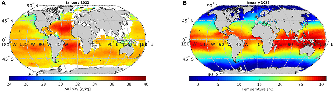
Figure 1. SMOS global SSS map averaged over January 2012 (A) along with a global SST map derived from OSTIA (B).

The Argo ISAS dataset provided gridded fields of temperature and salinity taken entirely from in-situ sources and spans the years from 2002 to 2015. Monthly data for salinity and temperature were obtained to a depth of 1975 dbar in 58 levels (Gaillard et al., 2016; Kolodziejczyk et al., 2017). We use Argo ISAS datasets for SSS and SST as a reference by which we compare satellite-derived formation rates from SMOS SSS and OSTIA SST.

The National Oceanography Centre Southampton (NOCS) produced datasets for latent and sensible heat fluxes. Their version 2 heat flux dataset includes both the radiative and turbulent heat budgets of the surface ocean derived mainly from in-situ observations made by Voluntary Observing Ships using bulk formulas (Berry and Kent, 2009).

Evaporation and precipitation are taken from the Objectively Analysed Air-sea Fluxes (OAFlux) and the Climate Prediction Centre's morphing method (CMORPH) datasets, respectively. The National Oceanic and Atmospheric Administration (NOAA) produced both datasets (Joyce et al., 2004; Yu et al., 2008). The CMORPH dataset is a high spatio-temporal resolution dataset derived from a blend of satellite passive microwave and infrared scans (Joyce et al., 2004). OAFlux is an optimal blend of three atmospheric re-analyses and satellite retrievals from microwave, infrared, radiometre, scatterometre, and rainfall measurement missions.

For all datasets, we consider a temporal domain spanning 3 years from 2012 to 2014 in order to see seasonal and inter-annual variability in water mass formation. All data products have a monthly resolution and are remapped to a 1° × 1° spatial resolution.

3. Methodology

We follow the method outlined by Speer and Tziperman (1992) in order to calculate water mass formation via air-sea fluxes of heat and freshwater.

3.1. Density-Flux, Transformation, and Formation

The transformation of water at a specific density is a function of the density flux at the surface of the ocean and it defines a cross-isopycnal volume flux. This can either be a movement of water to different densities—considering fixed isopycnals—or fluxes of heat and freshwater at the surface of the ocean causing a change in density. The following equations disregard advection and density changes that can occur due to vertical mixing effects at the base of the mixed layer.

The subsequent relation gives the density flux at the sea surface:

$\begin{array}{ll}f(x,y,t)=\frac{-\alpha H}{C_p}+\rho (0,T)\frac{\beta (W.S)}{1-S}& (1)\end{array}$

Where,

$\begin{array}{ll}\alpha =-\frac{1}{\rho }\frac{\partial \rho }{\partial T},\beta =\frac{1}{\rho }\frac{\partial \rho }{\partial S}& (2)\end{array}$

Equation (2) shows the coefficients of thermal expansion (α) and haline contraction (β), respectively. ρ(S, T) is the density, T and S are SST and SSS, respectively. H is the air-sea heat flux and W is evaporation minus precipitation (E–P), better known as the freshwater flux. C_p is the specific heat capacity of water at 4,000 JK⁻¹kg⁻¹. The resulting surface density flux (f(x,y,t)) is then given in kgm⁻²s⁻¹. Equation (1) can be expressed as f(i,j,m) when referring to latitudes, longitudes and months, respectively.

To derive a mathematical expression for water mass formation one must first define a transformation (i.e., the volume flux through a specific isopycnal). Formation would then be an accumulation or loss of water between two adjacent density surfaces. The volume flux through a specific density surface (transformation) is:

$\begin{array}{ll}\overline{F(\rho )}==\frac{1}{T\rho }{\displaystyle \int dt}{\displaystyle \iint dA}\delta \left(\rho -{\rho }^{\prime }\right)f(x,y,t)& (3)\end{array}$

Note that the transformation F is a function of density and hence temperature and salinity. The over-bar on $\overline{\mathit{\text{F(}}\rho \mathit{\text{)}}}$ represents an average over T = 1 year and the outcrop density = 1 kgm⁻³. As transformation is a volume flux, it is given in m³s⁻¹ or rather in Sverdrups (1 Sv = 10⁶m³s⁻¹). δ is the delta function being equal to 1 or 0 depending on whether one is within the area of the outcropping isopycnal in question (ρ = ρ′) or not (ρ ≠ ρ′). If δ is 1 the equation proceeds to take the area integral of the surface density flux (f(x,y,t)) within the area of the outcropping isopycnal (ρ_θ).

The formation is then given by a rate of change of transformation given by:

$\begin{array}{ll}\overline{M(\rho )}=-[\overline{F({\rho }^2)}-\overline{F({\rho }^1)}]& (4)\end{array}$

where the over-bar indicates an annual average. ρ² and ρ¹ represent two isopycnals with ρ located in between, such that ρ¹ < ρ < ρ². Formation then describes the convergence (positive M) or divergence (negative M) of transformation between the isopycnals ρ¹ and ρ².

At all grid points (i, j), we initially calculate f(i,j,m) (i.e., the monthly surface density flux). As the datasets are spatio-temporally discontinuous, calculations for transformation and formation are discretised. The integrals over area and time are replaced with a summation over the grid points (i, j) which fall into the area of the outcropping isopycnal or isotherm and isohaline. We achieve this by specifying bin widths of ρ, θ, and S at 1 kgm⁻³, 0.5°C and 0.1 PSU, respectively. We also use a boxcar sampling function that is 1 within the outcropping area and 0 otherwise.

Every grid point (i, j) and every time step (when discretised) has a specific surface density flux associated with it. However, transformation and formation are only a function of density (or θ–S) and thus give no spatial information. The geographic pattern of regions of formation gives insight into the spatial and temporal variability of water masses in geographic space.

3.2. Formation in Geographic Space

The spatial pattern of formation was not considered in the study performed by Speer and Tziperman (1992), therefore, the following formulations are taken from Brambilla et al. (2008). They defined a spatial formulation of formation and transformation to study the Mode Waters in the subpolar gyre.

They calculated the formation at every time step, through the use of transformation at every time step:

$\begin{array}{ll}{M}_m(\rho )=-\left[F({\rho }^2)-F({\rho }^1)\right]& (5)\end{array}$

and dividing this value by the region of the outcropping isopycnal in question R(ρ),

$\begin{array}{ll}{S}_{i,j,m}(\rho )=\frac{M_m(\rho )}{R_m(\rho )}\forall i,j{R}_m(\rho )& (6)\end{array}$

they arrived at a formulation for the spatial representation of formation (S_{i, j, m}(ρ)), at every grid point and time step. A summation of this value over all time steps provides an annual average of S_{i, j, m}(ρ).

$\begin{array}{ll}\overline{S_{i,j}(\rho )}={\displaystyle \sum _{m=1}^{12}}{S}_{i,j,m}(\rho )& (7)\end{array}$

Geographic representation of formation is practically done by defining a bounding box on a θ–S diagram. We define these bounding boxes to span 2°C and 0.5 PSU and centre around the visually identified point of peak formation. All positive formation pixels which lie within the box are then converted into geographic coordinates via (Equations 5–7).

3.3. Uncertainty Analysis—Methodology

SMOS and OSTIA, like any other remote sensing dataset, suffer from biases and inaccuracies due to intrinsic retrieval challenges (Font et al., 2010; Donlon et al., 2012). By perturbing the satellite SSS and SST data at every grid point, we can propagate these perturbations through to estimates of density flux, transformation and ultimately formation and compute statistics. This enables us to understand how uncertainties in the satellite datasets translate to uncertainties in the rates and location of water mass formation.

We use a Monte-Carlo simulation to introduce random perturbations in the satellite-derived datasets. We use a vector to store these random variables with a length equal to the number of Monte-Carlo realisations. We centre the random variables on the original SSS and SST values within a Gaussian distribution. They have a standard deviation close to the prescribed accuracy of the satellite SSS and SST datasets. 500 Monte-Carlo realisations are chosen for the subsequent analysis. The Monte-Carlo simulation takes the following form:

$\begin{array}{ll}SSS,SS{T}_{i,j,m}(n)=SSS,SS{T}_{i,j,m}+\text{x}·s_{SSS,SST}& (8)\end{array}$

where x is a uniformly distributed random vector, n is the number of Monte-Carlo realisations and s is the prescribed standard deviation. s is chosen based on a comparison between SMOS/OSTIA and Argo ISAS. To show how respective errors in SSS and SST influence uncertainty in estimates of formation, we alternately eliminate their prescribed uncertainties.

4. Results

Results for formation are computed over the North Atlantic (0°–44°N, 90.5°–0.5°W), North Pacific (5°S-59°N, 120°–240°E), and Southern Ocean (79.5°–40.5°S, with longitudes encircling the entire Southern Ocean). The respective regions are highlighted with black boxes in Figure 2. The area integral of the surface density flux results in the volume transport through each isopycnal (transformation) from 20 to 28 kgm⁻³—the density range considered in the current study. Formation is then given by the net accumulation or loss of water between successive density surfaces. By partitioning the relative influences of SSS and SST on density, formation can also be visualised in θ–S space.

FIGURE 2

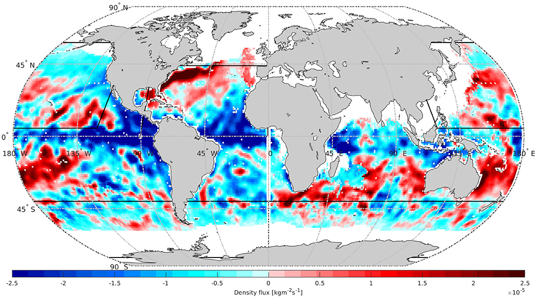
Figure 2. Annual averaged surface density flux for the year 2012 calculated using SMOS SSS and OSTIA SST. The black boxes represent the boundaries defined for the North Atlantic (0°–44°N, 90.5°–0.5°W), the North Pacific (5°S–59°N, 120°–240°E) and the Southern Ocean (79.5°–40.5°S, with longitudes encircling the entire Southern Ocean). Missing density flux estimates (indicated in white) are related to issues of satellite salinity retrieval due to Radio Frequency Interference or signal contamination from land contiguity.

4.1. Surface Density Flux

The global surface density flux is calculated as an annual average over 2012 (Figure 2). The figure shows the tendency of water to lose or gain density based on processes and phenomena that act to vary the heat and freshwater fluxes over the surface of the ocean. The global maximum of surface density flux is located in the North Atlantic over the Gulf Stream at ~45° to 80°W and 30° to 45°N. The density gain over the western boundary currents is associated with strong evaporation. In the equatorial regions, a density loss is caused either by heating through incoming solar radiation or by freshening through precipitation. This can be seen by the strongly negative values of surface density flux < –0.8 kgm⁻² s⁻¹ in the eastern Equatorial Pacific. The patterns over the rest of the global ocean remain consistent with these observations. The strongest density gain is most apparent at mid latitudes associated with boundary currents.

4.2. Formation in θ–S Space

By separating density into the relative contributions from SSS and SST it is possible to visualise formation in the θ–S bivariate plane. Results are shown over the winter months in 2012. Isopycnals are superimposed ranging from 16 to 30 kgm⁻³ (Figure 3). We consider a temperature and salinity range of 0–35°C and 27–39 PSU. This is sufficient to capture formation for the entire area of all basins studied. Looking at formation on a θ–S diagram allows for a greater degree of comparison with both literature and in-situ derived formation estimates. It also allows for a deeper diagnosis into the distribution and dynamics of formation estimated solely through satellite datasets. In Figure 4, the seasonal water mass formation evolution for the various satellite-driven inputs in the three basins is shown.

FIGURE 3

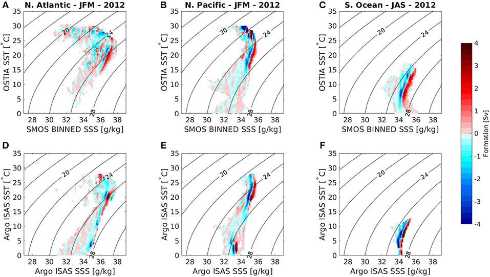
Figure 3. Formation in θ–S space for the North Atlantic (left), North Pacific (middle) and Southern Ocean (right), derived from SMOS SSS and OSTIA SST (A–C) and Argo ISAS SSS and SST (D–F) averaged over the winter months in 2012.

FIGURE 4

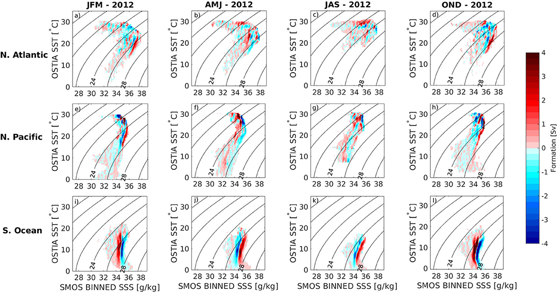
Figure 4. Seasonal evolution of formation for the North Atlantic (a–d), North Pacific (e–h), and Southern Ocean (i–l), averaged over winter (JFM), spring (AMJ), summer (JAS), and autumn (OND) of the year 2012.

In the North Atlantic (Figure 3A), two distinct peaks of positive formation are visible from both the satellite and in-situ datasets. For Argo ISAS the extent of the ridge differs by 0.3 PSU and 1.5°C from SMOS-OSTIA. Both dataset combinations peak in formation within this ridge at ~36.9 PSU and 20.5°C. The same ridge in θ–S space was associated with the properties of the Gulf Stream by Sabia et al. (2014). This matches the geographic location of the EDW (Worthington, 1958).

In the North Pacific, the peak formation based on SMOS-OSTIA is centred at 17°C and 35 PSU as shown in Figure 3B. Based on Argo ISAS, the peak formation is centered at the same salinity but the temperature is ~3°C warmer. Looking at the seasonal distribution (Figures 4e–h), this particular water mass peaks in the autumn and winter months (OND-JFM) and matches the θ–S location of North Pacific STMW (Masuzawa, 1969).

McCartney (1977) defined two water masses in the Southern Ocean north of the sub-Antarctic front, close to the Drake Passage in the South Atlantic. He defined a warmer, saltier water mass at 15°C and 35 PSU and a colder, fresher water mass at 4°C and 34.2 PSU. The formation derived from Argo ISAS shows only a single peak at 7°C and 34 PSU. The formation derived from SMOS-OSTIA, on the other hand, captures two distinct water masses in the Southern Ocean. The first is slightly colder and fresher at 10°C and 34.4 PSU; the second is warmer and more saline at 12.5°C and 35.5 PSU. Peak formation in each season spans a specific θ–S range. These peaks are indicated by small black boxes in Figures 5a–c (see section 3.2). To compare the satellite-derived properties with literature estimates, we indicate the literature-based properties by yellow dots. Overall, there is a remarkable agreement between the satellite-derived peak formation θ–S ranges and the Mode Water properties from literature. Based on our defined peak formation properties, we can now map the formation peaks into geographic space (Figures 5d–f).

FIGURE 5

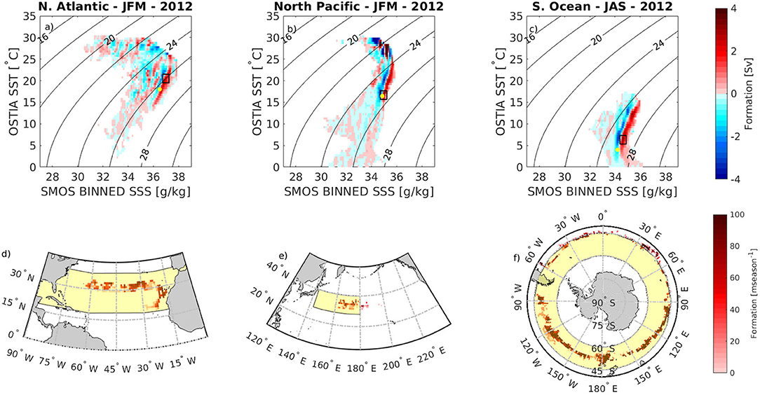
Figure 5. Averaged formation over the winter season in the North Atlantic (a), North Pacific (b) and Southern Ocean (c). Yellow dots (a–c) indicate literature properties of Mode Water within the respective basins. Maps of positive water mass formation are shown in (d–f) with the approximate geographic literature locations shaded in yellow (Worthington, 1958; McCartney, 1977, 1982; Hanawa and Hoshino, 1988; Yasuda and Hanawa, 1997; Hanawa and Yoritaka, 2001).

In the North Atlantic, peak winter formation occurs close to the subtropical gyre as shown in Figure 5d. This agrees well with the literature-based formation region (yellow shading in Figure 5d; Worthington, 1958; Hanawa and Talley, 2001).

Recent work using data from a 2000 to 2015 Argo climatology has shown that the location of core EDW conservative temperature and absolute salinity contours lie eastward relative to our satellite-derived geographic location of peak winter formation in the North Atlantic (Worthington, 1958; Feucher et al., 2019). This discrepancy could be due to sensing of additional processes by the superior spatial coverage of satellites.

In the North Pacific, the satellite-derived Mode Water properties agree remarkably well with literature-based properties of the North Pacific STMW (Figure 5b; Masuzawa, 1969; Feucher et al., 2019). The geographic location of the formation peak also corresponds well with the qualitative estimates of the North Pacific STMW formation area from literature (Masuzawa, 1969; Hanawa and Suga, 1995).

The position of the Southern Ocean water mass (Figure 5f) fits with the account of McCartney (1977) who found the coldest and freshest water mass just west of the Drake Passage. The core temperatures and salinities of the colder SAMW from literature (yellow dot in Figure 5c) and peak winter satellite-derived formation in θ–S coordinates differ slightly, perhaps reflecting the sparse surface observations in the Southern Ocean and as such poor heat flux estimates for the region (Josey et al., 1999; Kubota et al., 2003; Dong et al., 2007). Accurate air-sea flux estimates are critical for the estimation of water mass formation, especially in the Southern Ocean. Cerovečki et al. (2011) recently compared air-sea flux estimates in the Southern Ocean from a variety of sources. They reduced biases in a reanalysis product using adjustments from the Southern Ocean State Estimate (SOSE). The bias reduction showed that SOSE is a possible source of high-resolution fields of air-sea fluxes that are needed for an accurate estimation of water mass formation in the Southern Ocean. Figures 6–8 describe the inter-annual variability of seasonal formation in the North Atlantic, North Pacific and Southern Ocean. As in Figure 5, we mark the SSS and SST ranges of the peak formation of EDW, North Pacific STMW and SAMW during the autumn and winter months (black boxes) and compare them to the literature-based properties (yellow dots). In general, the satellite-derived formation peaks agree better with the literature-based water mass properties during the winter rather than autumn (Hanawa and Talley, 2001). The year 2013 represents the greatest agreement between literature properties of the EDW and satellite-derived peak water mass formation in both winter and autumn. The deviation between literature-based Mode Water properties and satellite-derived estimates for peak formation is greatest in 2014 in all three basins. For a better overview, we also present a comparison between the properties of satellite-derived formation peaks and the literature-based Mode Water properties in Table 1. Figure 9 shows spatial patterns of formation derived from SSS and SST ranges defined for the North Atlantic formation peak in winter (JFM). Figure 9 is the geographic equivalent to Figure 6. The geographic formation is seen to closely match literature in 2013, where spatial patterns of formation lie closer to the Gulf Stream (Figure 9; Worthington, 1958; Hanawa and Talley, 2001).

FIGURE 6

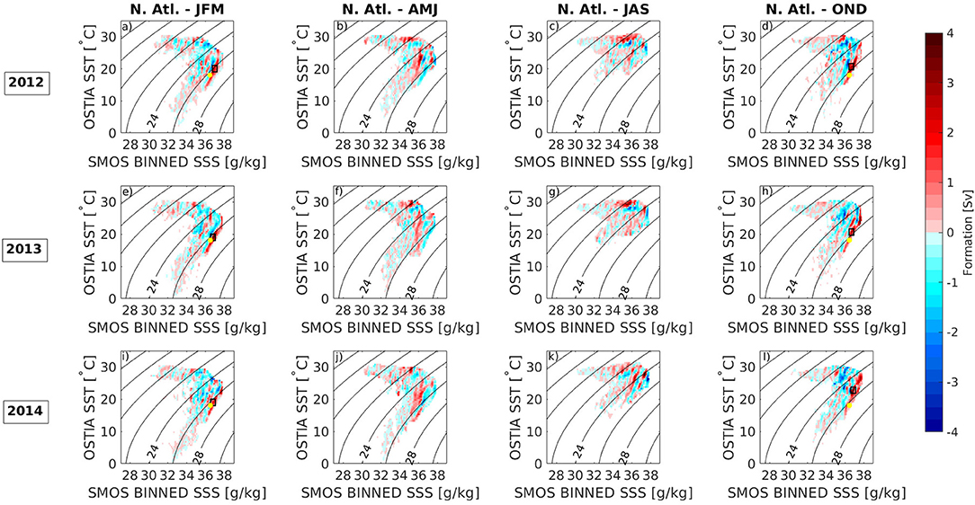
Figure 6. Seasonal formation from the North Atlantic in θ–S space over the years 2012 (a–d), 2013 (e–h), and 2014 (i–l). The four panels from left to right at each year indicate winter (JFM), spring (AMJ), summer (JAS), and autumn (OND), respectively. The yellow dots on the figures in the left and right most columns (JFM and OND) show the literature properties of the EDW (Worthington, 1958).

FIGURE 7

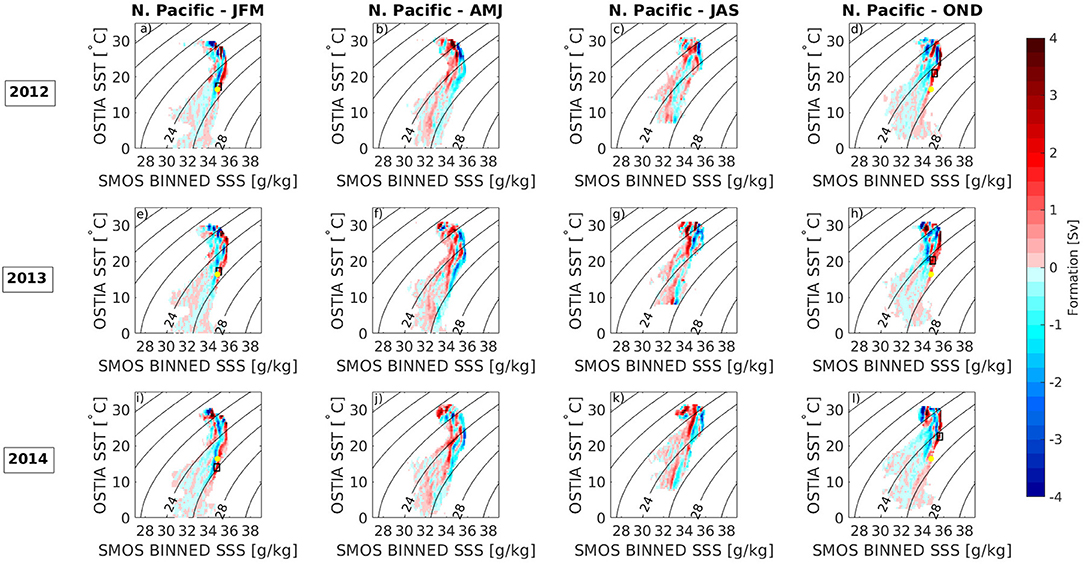
Figure 7. Same as Figure 6 but for the North Pacific and the yellow dots in the left and right most columns (JFM and OND) show the literature properties of the North Pacific STMW (Hanawa and Hoshino, 1988; Yasuda and Hanawa, 1997; Hanawa and Yoritaka, 2001).

FIGURE 8

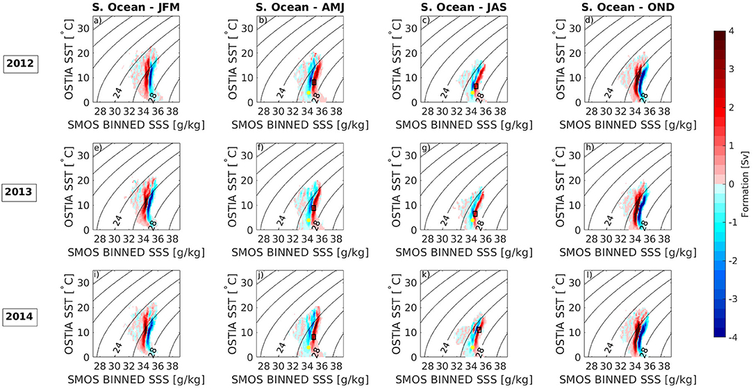
Figure 8. Same as Figure 6 but for the Southern Ocean and the yellow dots in the two centre columns (AMJ and JAS) show the literature properties of the SAMW (McCartney, 1977, 1982).

FIGURE 9

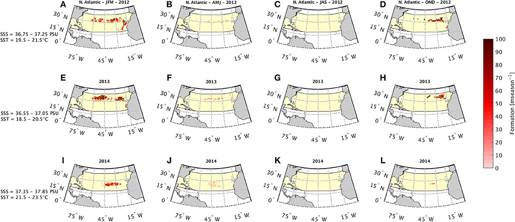
Figure 9. The geographic distribution of the water mass formation peak in the North Atlantic for the years 2012 (A–D), 2013 (E–H), and 2014 (I–L), and for the respective seasons winter (JFM), spring (AMJ), summer (JAS) and autumn (OND). The approximate geographic location of the EDW is shaded in yellow (Worthington, 1958; Hanawa and Talley, 2001).

TABLE 1

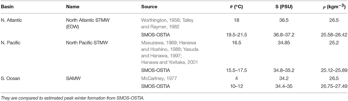
Table 1. Characteristic temperatures, salinities, and densities of Mode Waters in the North Atlantic, North Pacific, and Southern Ocean found in literature using in-situ data.

Satellite estimates—due to their superior coverage over in-situ datasets—represent an added value in understanding the variability of water masses in space and time, as compared to literature estimates.

5. Uncertainty Analysis–Results

5.1. Uncertainty of Water Mass Formation in σ-Space

As a first step, we estimate the uncertainty of the satellite-derived formation rates in σ-space. We use the Monte-Carlo simulations to propagate the respective uncertainties in SSS and SST to the formation estimates as described in section 3.3. We perform the Monte-Carlo simulations for all three basins and for the years 2013 and 2014. The uncertainty is visualised by the error bars, which are placed at 0.1 kgm⁻³ intervals. We also include formation estimates based on Argo ISAS data for comparison.

The satellite-derived formation peaks are shifted towards lighter densities with respect to the Argo-based estimates (Figure 10). This may reflect the fact that satellite-based salinity estimates are influenced by rain events (Ma et al., 2015). In 2013, the North Atlantic (Figure 10A) experiences a peak in positive formation at 26 kgm⁻³. However, in 2014 the closest peak of positive formation exists at 25.7 kgm⁻³. Peak positive formation at 25.7 kgm⁻³ is overestimated with respect to literature—which places an approximate range of 3.6 and 5.6 Sv at the lower and higher ends, respectively (Kwon, 2004; Maze et al., 2009).

FIGURE 10

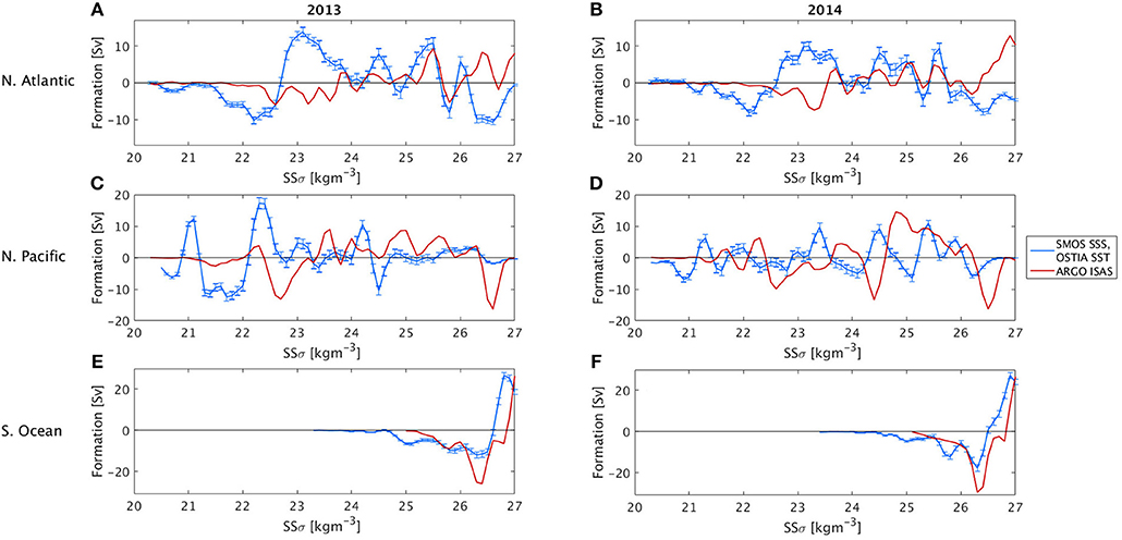
Figure 10. Annually averaged formation with error bars in σ-space for the year 2013 (left column) and 2014 (right column) over the North Atlantic (A,B), North Pacific (C,D), and Southern Ocean (E,F). The blue and red lines indicate formation in σ-space calculated using SMOS-OSTIA and Argo ISAS SSS and SST, respectively. Error bars indicate uncertainty over 500 Monte-Carlo realisations.

Masuzawa (1969) places the core density properties of the North Pacific STMW at 25.2 kgm⁻³. This approximately coincides with a peak in 2014 (Figure 10D) located at 25.3 kgm⁻³. In 2013, there is less agreement with literature as the closest positive formation peak occurs at 24.9 kgm⁻³ (Figure 10C) (Masuzawa, 1969).

According to McCartney (1977) there exist a warm and cold SAMW due to the nature of the sub-Antarctic Front. The coldest SAMW has a core density of 27.1 kgm⁻³ which lies closer to the positive formation peak in 2014 (Figure 10F) rather than 2013 (Figure 10E).

5.2. Uncertainty of Water Mass Formation in θ–S and Geographic Space

Formation in θ–S space as a result of the 500 Monte-Carlo simulations is presented in Figures 11a,b. We then apply a bounding box to each formation peak for each specific Monte-Carlo realisation. The mean and standard deviation are calculated over the entire ensemble of formation realisations. Thereafter, we compute the respective geographic distribution for all θ–S diagrams (Figures 11c,d).

FIGURE 11

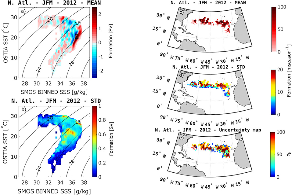
Figure 11. Mean and standard deviation of formation averaged over the North Atlantic during winter (JFM) in 2012 using 500 Monte-Carlo realisations. Mean and standard deviation of formation in θ–S space (a,b) and geographic space (c,d) is shown along with the uncertainty in the geographic extent of formation (e).

At every lat-lon point, we calculate the likelihood of formation occurrence as the percentage frequency at which positive formation occurs within the ensemble of geographic distributions (Figure 11e). Figure 11d represents the uncertainty in the formation estimates due to the uncertainty in the underlying satellite data. In Figure 11e, this uncertainty is translated into an uncertainty in the geographic distribution of a specific water mass.

Results show that after 500 Monte-Carlo simulations the winter mean formation peak centres at 37 PSU and 20°C. If the uncertainties in SMOS-OSTIA are not considered, the equivalent formation peak is shifted by 0.1 PSU and 0.5°C towards more saline and warmer waters, respectively (compare Figure 5a). These θ–S values are also further from the 36.5 PSU and 18°C found by Worthington (1958).

The geographic distribution agrees more with literature after a mean over 500 Monte-Carlo simulations. This results in a spread over a greater extent south of the Gulf Stream extension than in Figure 5d (Worthington, 1958; Hanawa and Talley, 2001; Maze et al., 2009).

6. Sensitivity Analysis

In this section, we intend to assess the relative contributions of θ and S to uncertainties in water mass formation. To do this, we consider uncertainties in only one of the datasets at a time. We compare these partial uncertainty estimates in θ–S (Figure 12) and geographic space (Figure 13) to the estimates of total uncertainty.

FIGURE 12

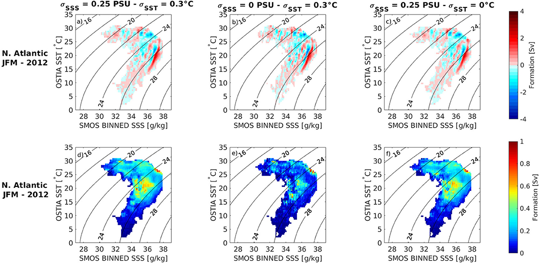
Figure 12. Mean (a–c) and standard deviation (d–f) of formation in θ–S space during the winter months (JFM) in 2012 over the North Atlantic after 500 Monte-Carlo realisations. The Monte-Carlo simulation was run three times with uncertainties considered in both SMOS SSS and OSTIA SST (first column), only OSTIA SST (second column) and only SMOS SSS (last column).

FIGURE 13

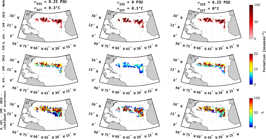
Figure 13. Mean (a–c) and standard deviation (d–f) of formation in geographic space after 500 Monte-Carlo realisations during the winter months (JFM) in 2012 over the North Atlantic, as well as the uncertainty in the geographic distribution over the 500 Monte-Carlo realisations (g–i). The Monte-Carlo simulation was run three times with uncertainties considered in both SMOS SSS and OSTIA SST (first column), only OSTIA SST (second column) and only SMOS SSS (last column).

When we consider only uncertainties in SST, the standard deviation of the Monte-Carlo ensemble is much smaller than the total standard deviation due to the combined uncertainties of SST and SSS (Figures 12d,e). Also, the mean after 500 Monte-Carlo simulations matches Figure 5a (i.e., assuming both SSS and SST to be perfectly known). When we consider only the uncertainties in SSS, the standard deviation of the Monte-Carlo ensemble closely resembles the total standard deviation (Figures 12d,f). The sensitivity experiment thus suggests that most of the uncertainty in the formation estimates can be attributed to uncertainties in SSS.

The extent of the formation area in geographic space is spread over a narrower latitudinal range when the uncertainties in SSS are ignored (Figure 13h). Therefore, we conclude that the uncertainties in SSS also dominate the uncertainties in geographic space—in terms of both the formation rate (Figures 13d–f) and the formation area (Figures 13g–i).

7. Conclusion

We calculate annual and seasonal water mass formation rates based on satellite SSS and SST in the North Atlantic, North Pacific and Southern Ocean for the years 2012 to 2014. The calculation is based on the variability of heat and freshwater fluxes (Walin, 1982; Speer and Tziperman, 1992). We further estimate how the uncertainty in the satellite data propagates into the final formation estimates. By looking at formation in three coordinate systems (σ, θ–S, and geographic space), we are able to constrain the properties and location of water mass formation more accurately than with a single coordinate system.

A comparison with previous literature-based Mode Water properties shows that the satellite-derived formation of Mode Waters is shifted towards higher salinities and higher temperatures. In addition to errors in the underlying satellite data, this shift could be explained by recent climate change. The satellites may also capture processes that cannot be captured by the poor spatial coverage of in-situ measurements (Marsh and New, 1996; Banks et al., 2000; Alfultis and Cornillon, 2001; Gulev et al., 2003). In comparison to Argo ISAS data, the satellite-derived water mass properties are shifted towards lower salinities. Work done on L-band microwave radiometres has shown that the effect of freshwater lenses on the ocean surface after a rain event interferes with the signals retrieved by the instrument (Boutin et al., 2013; Santos-Garcia et al., 2014; Ma et al., 2015).

To understand to which extent satellite SSS and SST uncertainties contribute to the final estimates of formation, we apply a Monte-Carlo simulation. We are able to assess the uncertainty in the formation rate estimates and also the uncertainty in the geographic distribution of the water mass. With this, we proceed to alternately eliminate prescribed uncertainties in the underlying datasets in a sensitivity analysis. We find that most of the uncertainty is accounted for by uncertainties in SSS. This highlights the need for frequent and increasingly accurate satellite SSS data for the estimation of water mass formation.

Future work can be planned around several research avenues of increasing complexity. The various types of satellite data sources can be expanded by evaluating the impact of additional satellites/sensors—namely satellite SSS from Aquarius/SMAP missions. The same would apply for the data sources regarding heat and freshwater fluxes; for the latter, the corresponding uncertainties can also be introduced. Then, a more thorough analysis of the seasonal-to-inter-annual variability of density flux, transformation and formation can be performed—trying to link the inferred variability with oceanographic/climatic processes. More complex formulations taking into account, for instance, advection processes (and their relationship to ocean currents) would give a broader picture into the water mass formation spatio-temporal evolution. A computer vision algorithm to automatically and reliably detect peaks in water mass formation and map the corresponding geographic location is currently under finalisation. Future work could also explore the possibility of retrieving information on the evolution of satellite-measured surface water masses through the use of well-known parametres such as the Turner angle or Brunt-Väisälä frequency.

This study emphasises how synoptic satellite measurements of SSS and SST can be extremely valuable to infer water mass characteristics from space. Sustained future satellite SSS and SST measurements, possibly at increased spatial resolution and with higher accuracy, are therefore much needed remote sensing observations. Algorithm improvements along the lines described above would render the process of estimating water mass features from space easily operational. A systematic and increasingly accurate estimation of water mass distribution and variability would shed light onto physical and biogeochemical oceanographic processes (ocean circulation, ocean/atmosphere exchanges, nutrients and carbon cycles, etc.) of major relevance for climate and society at large.

Author Contributions

AP: extended work initially done by MK under the supervision of RS and the code written by LC. RS: supervisor of AP and previous supervisor of MK. MK: trainee at ESRIN during 2010–11, started work on topic under supervision of RS. LC: software engineer wrote code formalising model initially found by MK in literature. DF: main supervisor of AP and manager of project.

Funding

This work was supported by the European space agency as part of Young Graduate Traineeship.

Conflict of Interest Statement

RS was employed by Telespazio-Vega UK Ltd.

The remaining authors declare that the research was conducted in the absence of any commercial or financial relationships that could be construed as a potential conflict of interest.

References

Alfultis, M. A., and Cornillon, P. (2001). A characterization of the north atlantic stmw layer climatology using world ocean atlas 1994 data. J. Atmosp. Ocean. Techn. 18, 2021–2037. doi: 10.1175/1520-0426(2001)018<2021:ACOTNA>2.0.CO;2

CrossRef Full Text | Google Scholar

Banks, H. T., Wood, R. A., Gregory, J. M., Johns, T. C., and Jones, G. S. (2000). Are observed decadal changes in intermediate water masses a signature of anthropogenic climate change? Geophys. Res. Lett. 27, 2961–2964. doi: 10.1029/2000GL011601

CrossRef Full Text | Google Scholar

BEC (2018). Smos-bec ocean products description. Technical report, Barcelona Expert Center, Barcelona.

Google Scholar

Berry, D. I., and Kent, E. C. (2009). Air-sea fluxes from ICOADS: the construction of a new gridded dataset with uncertainty estimates. Int. J. Climatol. 31, 987–1001. doi: 10.1002/joc.2059

CrossRef Full Text | Google Scholar

Boutin, J., Martin, N., Reverdin, G., Yin, X., and Gaillard, F. (2013). Sea surface freshening inferred from SMOS and ARGO salinity: impact of rain. Ocean Sci. 9, 183–192. doi: 10.5194/os-9-183-2013

CrossRef Full Text | Google Scholar

Boutin, J., Martin, N., Yin, X., Font, J., Reul, N., and Spurgeon, P. (2012). First assessment of SMOS data over open ocean: part II—sea surface salinity. IEEE Trans. Geosci. Remote Sens. 50, 1662–1675. doi: 10.1109/TGRS.2012.2184546

CrossRef Full Text | Google Scholar

Brambilla, E., Talley, L. D., and Robbins, P. E. (2008). Subpolar mode water in the northeastern atlantic: 2. origin and transformation. J. Geophys. Res. 113:C04026. doi: 10.1029/2006JC004063

CrossRef Full Text | Google Scholar

Cerovečki, I., Talley, L. D., and Mazloff, M. R. (2011). A comparison of southern ocean air–sea buoyancy flux from an ocean state estimate with five other products. J. Clim. 24, 6283–6306. doi: 10.1175/2011JCLI3858.1

CrossRef Full Text | Google Scholar

Dong, S., Gille, S. T., and Sprintall, J. (2007). An assessment of the southern ocean mixed layer heat budget. J. Clim. 20, 4425–4442. doi: 10.1175/JCLI4259.1

CrossRef Full Text | Google Scholar

Donlon, C. J., Martin, M., Stark, J., Roberts-Jones, J., Fiedler, E., and Wimmer, W. (2012). The operational sea surface temperature and sea ice analysis (OSTIA) system. Remote Sens. Environ. 116, 140–158. doi: 10.1016/j.rse.2010.10.017

CrossRef Full Text | Google Scholar

Entekhabi, D., Njoku, E. G., O'Neill, P. E., Kellogg, K. H., Crow, W. T., Edelstein, W. N., et al. (2010). The soil moisture active passive (SMAP) mission. Proc. IEEE 98, 704–716. doi: 10.1109/JPROC.2010.2043918

CrossRef Full Text | Google Scholar

Feucher, C., Maze, G., and Mercier, H. (2019). Subtropical mode water and permanent pycnocline properties in the world ocean. J. Geophys. Res. Oceans 124, 1139–1154. doi: 10.1029/2018JC014526

CrossRef Full Text | Google Scholar

Font, J., Boutin, J., Reul, N., Spurgeon, P., Ballabrera-Poy, J., Chuprin, A., et al. (2012). SMOS first data analysis for sea surface salinity determination. Int. J. Remote Sens. 34, 3654–3670. doi: 10.1080/01431161.2012.716541

CrossRef Full Text | Google Scholar

Font, J., Camps, A., Borges, A., Martín-Neira, M., Boutin, J., Reul, N., et al. (2010). SMOS: The challenging sea surface salinity measurement from space. Proc. IEEE 98, 649–665. doi: 10.1109/JPROC.2009.2033096

CrossRef Full Text | Google Scholar

Gaillard, F., Reynaud, T., Thierry, V., Kolodziejczyk, N., and von Schuckmann, K. (2016). In situ–based reanalysis of the global ocean temperature and salinity with ISAS: variability of the heat content and steric height. J. Clim. 29, 1305–1323. doi: 10.1175/JCLI-D-15-0028.1

CrossRef Full Text | Google Scholar

Gordon, A. L., Lutjeharms, J. R., and Gründlingh, M. L. (1987). Stratification and circulation at the agulhas retroflection. Deep Sea Res. Part A. Oceanog. Res. Papers 34, 565–599.

Google Scholar

Gulev, S. K., Barnier, B., Knochel, H., Molines, J.-M., and Cottet, M. (2003). Water mass transformation in the north atlantic and its impact on the meridional circulation: insights from an ocean model forced by ncep–ncar reanalysis surface fluxes. J. Clim. 16, 3085–3110. doi: 10.1175/1520-0442(2003)016<3085:WMTITN>2.0.CO;2

CrossRef Full Text | Google Scholar

Hanawa, K., and Hoshino, I. (1988). Temperature structure and mixed layer in the kuroshio region over the izu ridge. J. Mar. Res. 46, 683–700.

Google Scholar

Hanawa, K., and Suga, T. (1995). “A review on the subtropical mode water in the north pacific (npstmw),” in Biogeochemical Process and Ocean Flux in the Western Pacific (Tokyo: Terra Scientific), 613–627.

Google Scholar

Hanawa, K., and Talley, L. D. (2001). “Mode waters. Ocean circulation and climate,” in International Geophysics, eds G. Siedler and J. Church (Elsevier), 373–386.

Google Scholar

Hanawa, K., and Yoritaka, H. (2001). North pacific subtropical mode waters observed in long xbt cross sections along 32.5n line. J. Oceanog. 57, 679–692. doi: 10.1023/A:1021276224519

CrossRef Full Text | Google Scholar

Josey, S. A., Kent, E. C., and Taylor, P. K. (1999). New insights into the ocean heat budget closure problem from analysis of the soc air–sea flux climatology. J. Clim. 12, 2856–2880.

Google Scholar

Joyce, R. J., Janowiak, J. E., Arkin, P. A., and Xie, P. (2004). CMORPH: A method that produces global precipitation estimates from passive microwave and infrared data at high spatial and temporal resolution. J. Hydrometeorol. 5, 487–503. doi: 10.1175/1525-7541(2004)005<0487:CAMTPG>2.0.CO;2

CrossRef Full Text | Google Scholar

Kolodziejczyk, N., Prigent-Mazella, A., and Gaillard, F. (2017). ISAS-15 Temperature and Salinity Gridded Fields. SEANOE. doi: 10.17882/52367 seanoe.

CrossRef Full Text | Google Scholar

Kubota, M., Muramatsu, H., and Kano, A. (2003). Intercomparison of various surface turbulent heat flux fields. J. Clim. 1, 670–678. doi: 10.1175/1520-0442(2003)016<0670:IOVSLH>2.0.CO;2

CrossRef Full Text | Google Scholar

Kwon, Y.-O. (2004). North atlantic subtropical mode water: a history of ocean-atmosphere interaction 1961–2000. Geophys. Res. Lett. 31:L19307. doi: 10.1029/2004GL021116

CrossRef Full Text | Google Scholar

Ma, W., Yang, X., Yu, Y., Liu, G., Li, Z., and Jing, C. (2015). Impact of rain-induced sea surface roughness variations on salinity retrieval from the aquarius/SAC-d satellite. Acta Oceanol. Sin. 34, 89–96. doi: 10.1007/s13131-015-0660-5

CrossRef Full Text | Google Scholar

Marsh, R., and New, A. L. (1996). Modeling 18 water variability. J. Phys. Oceanog. 26, 1059–1080.

Google Scholar

Masuzawa, J. (1969). “Subtropical mode water,” in Deep Sea Research and Oceanographic Abstracts (Elsevier), 463–472.

Google Scholar

Maze, G., Forget, G., Buckley, M., Marshall, J., and Cerovecki, I. (2009). Using transformation and formation maps to study the role of air–sea heat fluxes in north atlantic eighteen degree water formation. J. Phys. Oceanog. 39, 1818–1835. doi: 10.1175/2009JPO3985.1

CrossRef Full Text | Google Scholar

McCartney, M. (1977). Subantarctic mode water. Voyage Discov. Deep Sea Res. 24, 103–119.

Google Scholar

McCartney, M. S. (1982). The subtropical recirculation of mode waters. J. Mar. Res 40, 427–464.

Google Scholar

Provost, C., Escoffier, C., Maamaatuaiahutapu, K., Kartavtseff, A., and Garçon, V. (1999). Subtropical mode waters in the south atlantic ocean. J. Geophys. Res. Oceans 104, 21033–21049.

Google Scholar

Roemmich, D., and Cornuelle, B. (1992). The subtropical mode waters of the south pacific ocean. J. Phys. Oceanog. 22, 1178–1187. doi: 10.1002/2014JC010120

CrossRef Full Text | Google Scholar

Sabia, R., Klockmann, M., Fernández-Prieto, D., and Donlon, C. (2014). A first estimation of SMOS-based ocean surface t-s diagrams. J. Geophys. Res. Oceans 119, 7357–7371.

Google Scholar

Santos-Garcia, A., Jacob, M. M., Jones, W. L., Asher, W. E., Hejazin, Y., Ebrahimi, H., et al. (2014). Investigation of rain effects on aquarius sea surface salinity measurements. J. Geophys. Res. Oceans 119, 7605–7624. doi: 10.1002/2014JC010137

CrossRef Full Text | Google Scholar

Sen, A., Kim, Y., Caruso, D., Lagerloef, G., Colomb, R., and Vine, D. L. (2006). “Aquarius/SAC-d mission overview,” in Sensors, Systems, and Next-Generation Satellites X, eds R. Meynart, S. P. Neeck, and H. Shimoda (Stockholme: SPIE), 1–10.

Google Scholar

Speer, K., and Tziperman, E. (1992). Rates of water mass formation in the north atlantic ocean. J. Phys. Oceanog. 22, 93–104.

Google Scholar

Talley, L. D., and Raymer, M. E. (1982). Eighteen degree water variability. J. Mar. Res. 40, 757–775.

Google Scholar

Walin, G. (1982). On the relation between sea-surface heat flow and thermal circulation in the ocean. Tellus 34, 187–195.

Google Scholar

Worthington, L. (1958). The 18° water in the sargasso sea. Deep Sea Res. 5, 297–305.

Google Scholar

Yasuda, T., and Hanawa, K. (1997). Decadal changes in the mode waters in the midlatitude north pacific. J. Phys. Oceanog. 27, 858–870.

Google Scholar

Yu, L., Jin, X., and Weller, R. A. (2008). Multidecade global flux datasets from the objectively analyzed air-sea fluxes (oaflux) project: latent and sensible heat fluxes, ocean evaporation, and related surface meteorological variables. OAFlux Project Tech. Rep. 74, 1–64.

Google Scholar

Zine, S., Boutin, J., Font, J., Reul, N., Waldteufel, P., Gabarro, C., et al. (2008). Overview of the SMOS sea surface salinity prototype processor. IEEE Trans. Geosci. Remote Sens. 46, 621–645. doi: 10.1109/TGRS.2008.915543

CrossRef Full Text | Google Scholar