Properties of Sediment Trap Catchment Areas in Fram Strait: Results From Lagrangian Modeling and Remote Sensing

Vertical particle fluxes are responsible for the transport of carbon and biogenic material from the surface to the deep ocean, hence understanding these fluxes is of climatic relevance. Sediment traps deployed in Fram Strait within the framework of the Arctic long-term observatory FRAM provide a time-series of vertical particle fluxes in a region of high CO₂ uptake. Until now the source area (catchment area) of trapped particles is unclear; however, lateral advection of particles is supposed to play an important role. This study presents a Lagrangian method to backtrack the origin of particles for two Fram Strait moorings equipped with sediment traps in 200 and 2,300 m depth by using the time-dependent velocity field of a high-resolution, eddy-resolving ocean-sea ice model. Our study shows that the extent of the catchment area is larger the deeper the trap and the slower the settling velocity. Chlorophyll-a concentration as well as sea ice coverage of the catchment area are highest in the summer months. The high sea ice coverage in summer compared to winter can possibly be related to a weaker across-strait sea level pressure difference, which allows more sea ice to enter the then well-stratified central Fram Strait where the moorings are located. Furthermore, a backward sea ice tracking approach shows that the origin and age of sea ice drifting through Fram Strait, partly responsible for vertical particle fluxes, varies strongly from year to year, pointing to a high variability in the composition of particles trapped in the moorings.

1. Introduction

The oceans play a critical role in the global carbon cycle through regulating the exchange of carbon dioxide between atmospheric and oceanic reservoirs. There are numerous interconnected mechanisms involved in this exchange: the biological carbon pump (Volk and Hoffert, 1985), the solubility pump, the microbial carbon pump (Jiao et al., 2010) and the lipid pump (Jónasdóttir et al., 2015). The biological carbon pump is perhaps the most widely studied and traditionally refers to the gravitational settling of particles produced in the surface to the ocean interior (Sarmiento and Gruber, 2006). It is comprised of two components: the soft-tissue pump (Volk and Hoffert, 1985) and the carbonate counter pump (Heinze and Maier-Reimer, 1991). The soft-tissue pump is the vertical transfer of photosynthetically fixed carbon dioxide into the ocean interior as organic particles (Sarmiento et al., 1988), that may be associated with inorganic ballast minerals (Klaas and Archer, 2002; Salter et al., 2010). The carbonate counter pump is related to the precipitation of calcium carbonate minerals that act as a source of CO₂ to the atmosphere over climatically-relevant timescales (Zeebe, 2012). The balance of these two processes thus governs the net sequestration of atmospheric CO₂ into the ocean interior (Antia et al., 2001; Salter et al., 2014) and thus has an important impact on global climate (Sarmiento and Toggweiler, 1984; Sabine et al., 2004; Kwon et al., 2009). In addition, through pelagic-benthic coupling (Graf, 1998), the biological carbon pump acts as the principal source of energy and nutrients to abyssal ecosystems (Billett et al., 1983; Rembauville et al., 2018). A good understanding of the mechanisms transferring biogenic particles from the surface to the deep-ocean and sediments is critical.

Early studies attempting to link surface properties like primary productivity to particle flux have provided evidence for fast one dimensional coupling (Deuser and Ross, 1980; Alldredge and Chris, 1988; Asper et al., 1992). However, it has been subsequently shown that horizontal advection of water may displace particles significantly from their place of production during sinking (Siegel and Deuser, 1997; Waniek et al., 2000, 2005). Lateral advection and variable settling velocities thus have the potential to significantly modify the spatial pattern of transmission of a surface signal to the ocean interior. Significant inputs of particles can be laterally advected from ocean margins and shelf systems and can be important for balancing regional biogeochemical budgets (Anderson and Ryabchenko, 2009; Burd et al., 2010). Mesoscale eddies have also been shown to shape planktonic particle distribution and influence export to the deep-ocean (Waite et al., 2016). Interpretation of flux data measured by moored sediment traps therefore relies on resolving these physical processes (Waniek et al., 2005).

In addition to horizontal fluid velocities, the consideration of particle settling velocities is critical to determine particle export trajectories from the surface ocean (e.g., Siegel et al., 1990; Waniek et al., 2000). Ballasting of particles by biogenic and lithogenic minerals can effect the transfer of organic material to the deep-ocean (Armstrong et al., 2001; Klaas and Archer, 2002). Laboratory experiments and field studies have indicated that mineral ballast can increase the density and settling velocity of particles (Fischer and Karakaş, 2009; Iversen and Ploug, 2010; Lombard et al., 2013). Lithogenic minerals in particular may modify the transfer of organic material to the bathypelagic (Ittekkot, 1993; Salter et al., 2010) and could be particularly important in the Arctic if aluminosilicate clays are entrained in the ice through suspension freezing over shallow topography. A wide variety of techniques has been used to determine particle settling velocities including laboratory settling columns, in-situ settling columns and imaging systems (Asper and Smith, 2003), temporal peak matching of particle flux profiles (Armstrong et al., 2009) and particle gel traps (McDonnell and Buesseler, 2010). These methods have generated a large range of settling velocities that vary between 5 and 2,700 m/d (McDonnell and Buesseler, 2010). Typically marine particles are considered to settle in the range of one to some meters per day for phytoplankton cells, hundreds of meters per day for aggregates and upwards of hundred to several thousand meters per day for fecal material (Waniek et al., 2000; Turner, 2002; Armstrong et al., 2009; McDonnell and Buesseler, 2010; Turner et al., 2014). Quantitative partitioning across different sinking fractions shows that both large, fast sinking particles and small, slow sinking particles can be important contributors to total organic matter flux (Peterson et al., 2005; Trull et al., 2008; Riley et al., 2012; Durkin et al., 2015) and is unsurprisingly related to planktonic ecosystem structure. Variability in sinking velocity classes and particle flux size-spectra has important implications for calculating particle trajectories.

Estimating the catchment area (according to Deuser et al., 1988 defined as the surface domain that contains all likely positions where particles entering the trap might come from) is not a trivial task, and a range of different methods and simplifications have been applied previously. Due to lack of availability of a full time-dependent 3D velocity field, several studies used the time dependent velocity profile measured by instruments attached to moorings to calculate particle trajectories (v. Gyldenfeldt et al., 2000; Waniek et al., 2000, 2005; Bauerfeind et al., 2009). This results in so called progressive vector diagrams, which are based on the assumption of spatial homogeneity of the horizontal velocity field around the trap. In these studies the resulting catchment area is described in terms of distance to the trap (e.g., Waniek et al., 2005, their Figure 5), but does not indicate the geographical location. Another approach was followed by Siegel et al. (2008), using a combination of geostrophic velocities derived from satellite altimetry, shipboard ADCP data and satellite-tracked surface drifters. Abell et al. (2013) used surface geostrophic currents derived from satellite altimetry and reconstructed a time dependent 3D velocity field by assuming that currents decrease linearly from the surface to 15% at 1,500 m depth to backtrack particles in time starting at the trap. Qiu et al. (2014) performed backward particle tracking for sediment traps located in the Ligurian Sea by using the time dependent 3D velocity field of an ocean model.

The FRontiers in Arctic Monitoring observatory (FRAM; Soltwedel et al., 2013) aims to establish a long-term observing infrastructure that is capable of detecting changes in the physical, chemical and biological properties of a rapidly changing Arctic Ocean. It is comprised of numerous observing components that include fixed point mooring arrays and seafloor observations, and also numerical ocean modeling. The instrumentation and autonomous sampling devices deployed on the observational components aim to provide continuous data-flow on the organic flux rates to the seafloor and the resulting impact on deep-sea communities. To link the variability in these phenomena to changes occurring in the surface ocean, it is necessary to take advantage of ocean models that realistically represent the circulation and hydrography of the region, as well as remote-sensing data products that can provide information on chlorophyll-a and ice-cover dynamics. The objectives of the present study are to (i) develop a particle tracking model to define catchment areas of sediment traps and (ii) constrain the temporal variability of sea ice coverage and chlorophyll-a distribution within the defined catchment areas.

2. Study Area, Methods, and Material

2.1. Study Area

The Fram Strait, located between Greenland and Svalbard (Figure 1A), is characterized by contrasting water masses. Warm and salty waters of Atlantic origin are carried northward by the West Spitsbergen Current (WSC, e.g., von Appen et al., 2016). A fraction of the Atlantic Water (AW) carried by the WSC recirculates in Fram Strait at around 79°N and continues to flow southward, forming the Return Atlantic Water (RAW), whereas the remaining part enters the Arctic Ocean via the Svalbard and Yermak branches. Along the Greenland continental shelf break, the East Greenland Current (EGC, e.g., de Steur et al., 2009) carries cold and fresh Polar Water (PW) as well as RAW southward. Sea ice is exported with the Transpolar Drift out of the Arctic through the Fram Strait. The sea ice export occurs at the western side of the strait, which is thus ice-covered year-round. The eastern part of the Fram Strait is ice-free year-round due to the presence of warm AW.

FIGURE 1

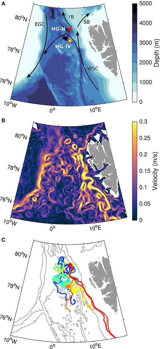
Figure 1. (A) Bathymetry in the Fram Strait region. Shown are the locations of the two moorings, HG-N (red star) and HG-IV (yellow star). Indicated are also major currents in the Fram Strait: West Spitsbergen Current (WSC), East Greenland Current (EGC), Yermak Branch (YB) and Svalbard Branch (SB). (B) Snapshot of simulated velocity in 100 m depth on 1 July 2009. (C) 115-day long backward trajectories of particles calculated with a settling velocity of 20 m/d released at HG-N in 2,300 m depth in the time period 1–14 July 2009. Each color indicates a different release date. Gray contours show the bathymetry at 1,000 m intervals.

In this study, we focus on moorings HG-IV and HG-N which are part of the FRAM Observatory (Figure 1A). HG-IV and HG-N are located in the central Fram Strait, southeast and northeast, respectively of the Molloy Deep, the deepest depression of Fram Strait. They are located in a region where warm AW recirculates westward.

2.2. Ocean-Sea Ice Model

Model output from the Finite-Element Sea-ice Ocean Model (FESOM) version 1.4 is used to calculate backward trajectories. FESOM is an ocean-sea ice model which solves the hydrostatic primitive equations in the Boussinesq approximation and is discretized with the finite element method (Wang et al., 2014; Danilov et al., 2015). Details on the coupling of the ocean and sea ice model can be found in Timmermann et al. (2009). In this study, we use a FESOM configuration that was optimized for Fram Strait, applying a mesh resolution of 1 km in this area (Wekerle et al., 2017). By comparing with the local Rossby radius of deformation (around 4–6 km in Fram Strait, e.g., von Appen et al., 2016) which is an indication of eddy size, this configuration can be considered as “eddy-resolving.” A snapshot of the simulated velocity in 100 m depth is shown in Figure 1B, revealing strong eddy activity. The simulation covers the time period 2000 until 2009. It is forced with atmospheric reanalysis data from COREv.2 (Large and Yeager, 2008), which includes sea surface wind and temperature, precipitation and snow, and longwave and shortwave radiation. River runoff is taken from the interannual monthly data set provided by Dai et al. (2009). A comparison with observational data (hydrography and velocity measured by a mooring array in Fram Strait) showed that the model performs well in reproducing circulation structure, eddy kinetic energy and hydrography (Wekerle et al., 2017).

2.3. Calculation of Backward Ocean Trajectories

To determine the catchment area of sediment traps deployed in Fram Strait, we used a Lagrangian particle tracking algorithm (see Appendix for details) and computed backward particle trajectories. This was done by reversing the flow field, i.e., particles were treated as if they were rising from the mooring location to the surface with a negative settling velocity, being horizontally displaced with the reversed horizontal velocity (vertical ocean velocities were neglected). Particles were advected with daily averaged horizontal model velocities from the FESOM simulation described above and a constant settling velocity¹ of either 120, 60, or 20 m/d. They were released at either 200 or 2,300 m depth (which is relatively close to the bottom), and tracked until they reached the surface. Thus, the duration of trajectories released at e.g., 2,300 m depth was 19, 38, and 115 days for settling velocities of 120, 60, and 20 m/d, respectively. The computation of backward particle trajectories was performed for two locations of moorings equipped with sediment traps in central Fram Strait, HG-N and HG-IV (indicated by stars in Figure 1A). Note that other starting positions or settling velocites can be implemented easily. Particles were released once per day during the time period 2002–2009, resulting in 2,920 trajectories. Considering the 12 experiments (two mooring positions, two depths of release, three settling velocities, see Table 1), altogether 35,040 trajectories were calculated. A time step of 1 h was used for the trajectory calculation, and thus hourly positions and corresponding temperature and salinity values were stored. A sensitivity test with smaller time steps revealed that a time step of 1 h is sufficient.

TABLE 1

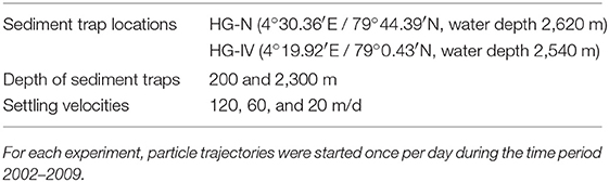
Table 1. Settings of 12 experiments performed in this study.

With this procedure, some assumptions and simplifications are made. By using the daily averaged velocity field, fluctuations on time scales less than a day are neglected. Note also that tides are not explicitly simulated in the FESOM configuration used in this study. Some Lagrangian codes include sub-grid scale turbulence by either adding a random velocity or by adding a random displacement of the particle position (e.g., Döös et al., 2011, 2017). This was not done in our study, which adds to the uncertainty in our experiments. Nonetheless, meso-scale variability is well reproduced in the ocean-sea ice model, as shown by Wekerle et al. (2017). Using constant settling velocities also increases the uncertainties in our calculations, which will be further discussed in section 4.4.

To quantify the spatial structure of the simulated catchment area, particle positions at the sea surface were binned into a spatial grid and then divided by the total number of particles to determine the fraction of collected particles originating from each grid box.

2.4. Measurements of Settling Velocities

During expedition PS99.2 with RV Polarstern to Fram Strait in summer 2016, intact aggregates were sampled using a marine snow catcher (MSC). On board, their settling velocities as well as size and composition were measured. The aggregates were individually transferred to a vertical flow chamber (Ploug et al., 2010) that was filled with GF/F filtered seawater collected from the same MSC and kept at in situ temperature. The x-,y-, and z-axis of each aggregate was measured in the vertical flow system using a horizontal dissection microscope and an ocular. The volume was thereafter calculated assuming an ellipsoid form, which was used to calculate the equivalent spherical diameter. To measure the sinking velocity, aggregates were placed in the middle of the flow chamber and upward flow was increased until the aggregate was floating one diameter above the net. The sinking velocity was thereafter calculated by determining the flow speed three times, and dividing the average of these measurements by the area of the flow chamber.

2.5. Calculation of Backward Sea Ice Trajectories

To determine sea ice source area and age of sea ice arriving in Fram Strait, a Lagrangian approach (ICETrack) was used that tracks sea ice backward in time using a combination of satellite-derived low resolution drift products. ICETrack has been used in a number of publications to examine sea ice sources, pathways, thickness changes and atmospheric processes acting on the ice cover (Krumpen et al., 2016; Damm et al., 2018; Peeken et al., 2018). The tracking approach works as follows: An ice parcel is tracked backward in time on a daily basis starting at Fram Strait. Tracking is stopped if (a) ice hits the coastline or fast ice edge, or (b) ice concentration at a specific location drops below 20% and we assume the ice to be formed.

2.6. Sea Ice Concentration Data

A sea ice concentration product provided by CERSAT is used in this study. It is based on 85 GHz SSM/I brightness temperatures, applying the ARTIST Sea Ice (ASI) algorithm. The product is available on a 12.5 × 12.5 km grid (Ezraty et al., 2007).

We use a weighted mean approach to estimate the sea ice coverage of the simulated catchment area. First, particle positions at the sea surface of all trajectory calculations conducted daily for the time period 2002–2009 are binned into the 12.5 × 12.5 km grid. As described in section 2.3, this amounts to altogether 2,920 trajectories per experiment, resulting in a climatological two-dimensional probability distribution for particle origin. Second, the ice coverage of the catchment area for each month of the time period 1998–2016 is computed by weighting the ice concentration of a grid box with the number of particles that reach the surface in that box. Using these probability distributions for calculating weighted means for sea ice coverage provides a more realistic estimate than simply integrating the surface property evenly over the areal extent of the catchment area.

2.7. Chlorophyll Concentration Data

Ocean color technique exploits the electromagnetic radiation emerging from the sea surface at different wavelengths of the visible wavelength region. The spectral variability of this signal defines the so called ocean color which is affected by the presence of phytoplankton. By comparing reflectances at different wavelengths and calibrating the result against in-situ measurements, an estimate of chlorophyll content can be derived. The Climate Change Initiative (CCI) of the European Space Agency (ESA) is a 2-part program aiming to produce “climate quality” merged data records from multiple sensors. The Ocean Color project within this program has a primary focus on chlorophyll in open oceans, using the highest quality of radiation measurements and merging process to date. This uses a combination of band-shifting to a reference sensor and temporally-weighted bias correction to align independent sensors into a coherent and minimally-biased set of reflectances. These are derived from standard level 2 products, calculated by the best-in-class atmospheric correction algorithms.

For the Arctic Ocean, the ESA Ocean Color CCI Remote Sensing Reflectance (merged, bias-corrected) data are used to compute surface chlorophyll-a concentration with a spatial resolution of 1 km² using the regional OC5ci chlorophyll algorithms. The Remote Sensing Reflectance data are generated by merging the measurements from SeaWiFS, MODIS-Aqua and MERIS sensors and realigning the spectra to that of the SeaWiFS sensor. The chlorophyll-a concentration is estimated from the OC5ci algorithm, a combination of the Case 1 OCI (Hu et al., 2012) and the Case 2 OC5 (Gohin et al., 2008) algorithms, developed at PML (Plymouth Marine Laboratory) within the Copernicus Marine Environment Monitoring Service (CMEMS). Units are expressed in mg m⁻³.

As in the case of sea ice coverage described above, we compute the chlorophyll-a content of the simulated catchment area as a weighted mean. Again, the catchment area computed from all trajectories calculated daily for the time period 2002–2009 is used. First, the chlorophyll-a data is interpolated to the sea ice grid (12.5 × 12.5 km resolution). Second, the chlorophyll-a concentration of a grid box is weighted with the number of particles that reach the surface in that box. As monthly means of chlorophyll-a concentration is available for the time period 1998–2016, we obtain a 19-year long time-series.

3. Results

3.1. Catchment Area of Particles Advected By Ocean Currents

Pathways of 14 particles released at HG-N (4°30.36′E/79°44.39′N) in 2300 m depth from 1 to 14 July 2009 sinking with a speed of 20 m/d are shown in Figure 1C. Particles travel distances between 540 and 950 km, and some of them reach the surface as far south as ~74.4°N. Most particles originate from south of the mooring position, indicating that they are carried by the northward flowing WSC. The particle trajectories exhibit strong eddying motions driven by the eddying velocity field, as seen in a snapshot of simulated velocity from 1 July 2009 (Figure 1B).

All particle positions at the sea surface are binned into a grid with a spacing of 24 × 24 km. The percentage of particles originating from each grid box for each of the 12 experiments listed in Table 1 is shown in Figure 2. For both moorings, HG-IV and HG-N, the simulated catchment area (here defined as the area where at least one particle reaches the surface) is larger the deeper the trap and the slower the settling velocity. This is expected since particles stay in the water column for a longer time period and are thus exposed to a greater extent to the currents. For all experiments, most particles originate from southeast of the mooring locations, which shows that they were carried by the northward flowing WSC. Particularly in the experiment with the deep trap and slow sinking rate (2,300 m depth and 20 m/d), the pattern of particle distribution reveals the two branches of the WSC, the inshore WSC located mainly between the 1,000 and 2,000 m isobaths, and the offshore branch that mainly follows the Knipovich Ridge. This is even more distinct for particles released at mooring HG-IV than at HG-N. Some of the particles originate from north of the mooring location, indicating the influence of the EGC and of the dynamic eddy field that leads to random movement of particles.

FIGURE 2

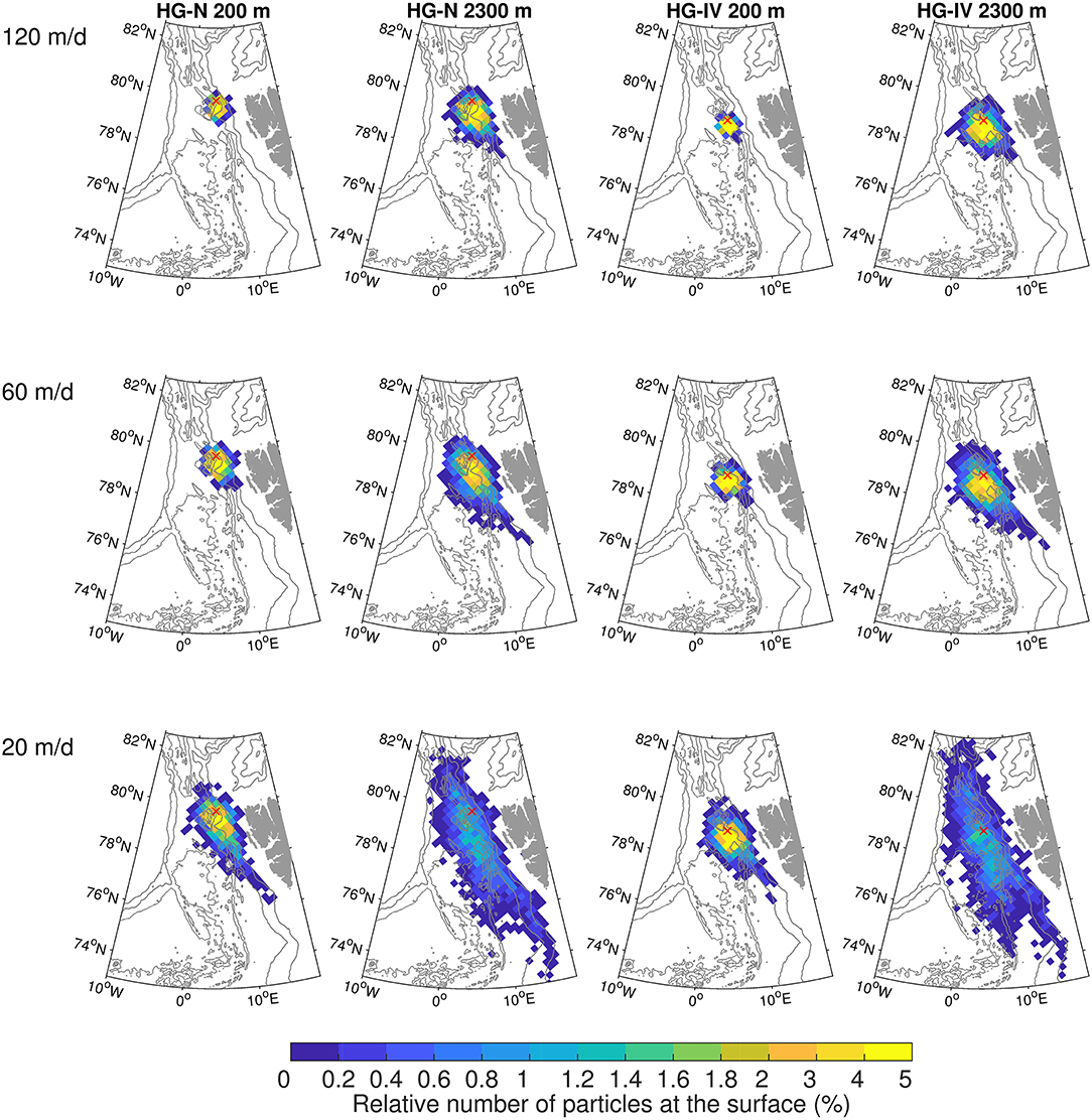
Figure 2. Relative number of particles (in %) reaching the surface in bins of 24 × 24 km size, originating from moorings HG-N and HG-IV at 200 and 2,300 m depth and assuming different settling velocities (120, 60, and 20 m/d). Particle positions at the sea surface are binned into the spatial grid and then divided by the total number of particles. The red cross indicates the mooring location. Gray contours show the bathymetry at 1,000 m intervals.

The trajectory path length is, as expected, highest in experiments 2,300 m depth/20 m/d, and reaches up to 1,000 km (Figure 3A). The mean/median path length in these experiments amounts to 560/550 km and 540/530 km in the case of HG-IV and HG-N, respectively. Particles reach the surface as far as ~74°N and ~82°N, with distances to the mooring locations of more than 400 km (Figure 3B). Mean / median distances to the mooring locations HG-IV and HG-N are 160/140 and 190/150 km, respectively. With a faster settling velocity of 60 m/d, trajectory path lengths up to 400 km are reached, and mean/median values amount to 200/190 km (HG-IV) and 190/180 km (HG-N). In the experiments with the shallow trap (200 m depth) and fast sinking rate of 120 m/d, the trajectory path length does not exceed 100 km, and mean / median trajectory path lengths of 18/15 km (HG-IV) and 22/19 km (HG-N) are reached.

FIGURE 3

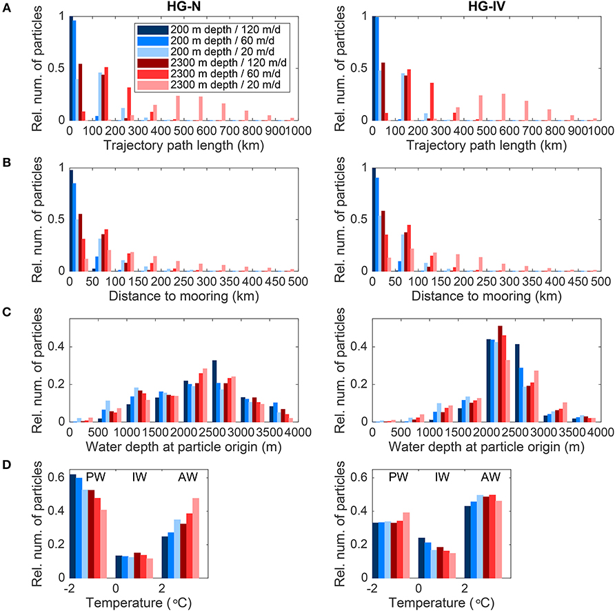
Figure 3. Histograms of (A) travel path length in km, (B) distance in km between particle location at the surface and sediment traps, (C) water depth at the particle origin and (D) temperature at the particle surface position for sediment traps (left) HG-N and (right) HG-IV, different depths of particle release (200 and 2,300 m) and settling velocities (120, 60, and 20 m/d). Abbreviations PW, IW, and AW stand for water masses Polar Water (T <0°C), Intermediate Water (0°C< T <2°C) and Atlantic Water (T>2°C), respectively.

For mooring HG-IV, most particles (the range is 69–90% in all 6 experiments) originate from areas with water depth deeper than 2,000 m, whereas for mooring HG-N, the percentage of particles originating from shallower regions is higher. It is noticeable, however, that for both moorings, almost no particles originate from shallow areas with depths between 0 and 500 m (Figure 3C).

A large fraction of particles trapped in mooring HG-N originates from areas characterized by PW (defined as waters with T < 0°C) at the surface (39–63% in all 6 experiments), and a smaller fraction of particles originates from areas with AW (defined as waters with T>2°C) at the surface (24–49%) (Figure 3D). This is opposite for mooring HG-IV with less particles originating from areas with PW (34–41%), and more particles originating from areas with AW (42–49%). Note that mooring HG-N is only located ~80 km northwest of HG-IV, but this difference already leads to differences in surface water mass properties of particles.

The seasonal variation in the particle distribution at the surface is rather low for all 12 experiments (Figure 4). Moreover, the spatial extent of the simulated catchment area does not vary strongly during the year and also on inter-annual timescales (Figures S1, S2). In fact, in terms of spatial extent, the amplitude of the seasonal cycle is lower than the difference between the 12 experiments.

FIGURE 4

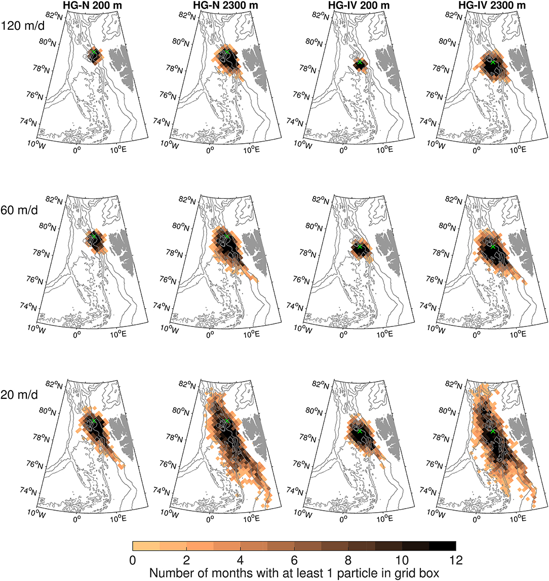
Figure 4. Seasonal distribution of the catchment area for sediment traps HG-N and HG-IV, different depths of particle release (200 and 2,300 m) and settling velocities (120, 60, and 20 m/d): For each grid box of size 24 × 24 km, the number of months is shown in which at least one particle reaches the surface. The green cross indicates the mooring location. Gray contours show the bathymetry at 1,000 m intervals.

3.2. Sea Ice Coverage and Chlorophyll-A Distribution in the Catchment Area

The ice coverage of the simulated catchment area shows significant inter-annual variability (Figure 5). In most years, it reaches values of up to ~20% for mooring HG-N and slightly lower values for mooring HG-IV. This rather low ice coverage indicates that large parts of the simulated catchment area of both moorings are located in the marginal ice zone characterized by low ice concentration or in areas characterized by Atlantic Water. However, in some years a particularly high ice coverage occurs (years 1998, 2003, 2008, 2009, 2012, 2013, and 2014). The seasonal cycle reveals a maximum in June, which will be further discussed in section 4.3.

FIGURE 5

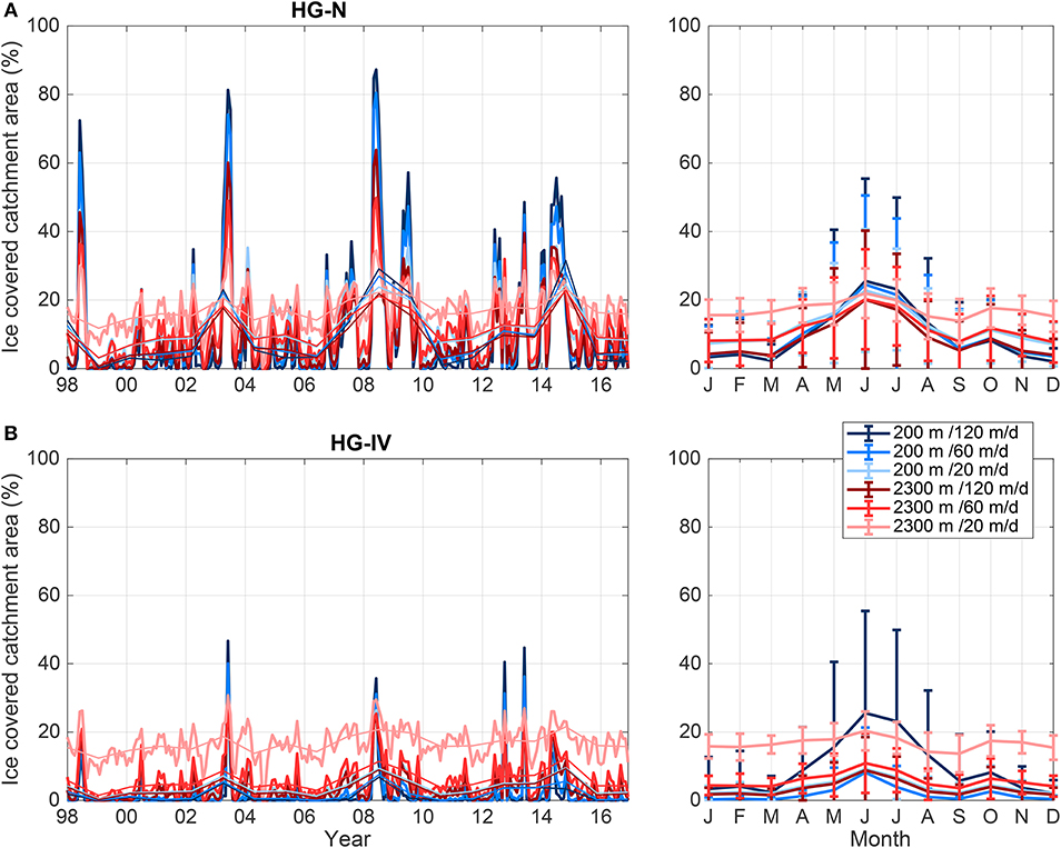
Figure 5. Monthly mean (thick lines) and annual mean (thin lines) ice coverage of the catchment area (in %) of sediment traps (A) HG-N and (B) HG-IV for the time period 1998–2016 (left) and its seasonal cycle (right). Error bars in the right panel show the standard deviation of the monthly mean values.

In addition to sea ice coverage, we also investigate the chlorophyll-a content of the simulated catchment area (Figure 6). Since ocean color measurements depend on light, they only provide values for open water and for the summer period (May to August). The catchment area obtained in the experiment with 2300 m water depth and 20 m/d settling velocity extends further to the south than all other experiments, and thus values up to September are available. The maximum chlorophyll-a concentration in the catchment area occurs in June in all experiments. The summer mean time series shows that there is significant inter-annual variability. For the HG-IV and HG-N catchment areas, chlorophyll-a concentration has increased in the recent years. The trend in summer chlorophyll-a concentration ranges between 0.014 and 0.02 mg/m³/year in the six HG-IV experiments, and between 0.017 and 0.022 mg/m³/year in the six HG-N experiments. This is consistent with the studies by Nöthig et al. (2015) and Cherkasheva et al. (2014). In particular, Cherkasheva et al. (2014) found a positive trend in Fram Strait chlorophyll-a concentration of 0.015 mg/m³/year for the years 1998–2009, and explained this with an increase in sea surface temperature and a decrease in Svalbard coastal ice.

FIGURE 6

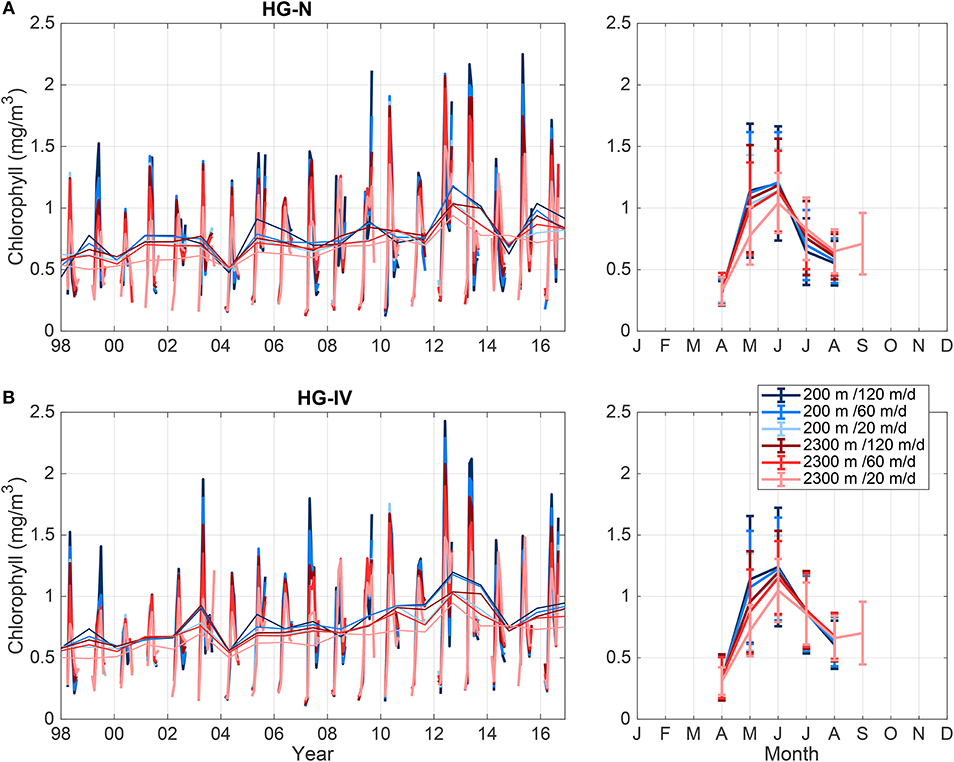
Figure 6. Monthly mean (thick lines) and summer mean (thin lines) chlorophyll-a distribution of the catchment area (mg m⁻³) of sediment traps (A) HG-N and (B) HG-IV for the time period 1998–2016 (left) and its seasonal cycle (right). Error bars in the right panel show the standard deviation of the monthly mean values. Note that data coverage is limited to the summer months.

The annual time series shows that years with high chlorophyll-a content in the simulated catchment area do not coincide with years with high sea ice coverage. This is expected since chlorophyll-a measurements are only available for ice-free waters. However, concerning the seasonal cycle, the maximum in sea ice coverage and chlorophyll-a concentration both occurs in June.

3.3. Catchment Area of Particles Carried by Sea Ice

The ice coverage of the simulated catchment areas of moorings HG-N and HG-IV is ~20%, indicating that both moorings are located in the marginal ice zone. Hence, sea ice plays an important role for vertical particle fluxes. Sea ice melting rates in Fram Strait are high due to the interaction of sea ice with warm Atlantic Water, and thus particles trapped by sea ice or organisms growing underneath sea ice contribute to vertical particle fluxes. How much sea ice contributes to sedimentation in Fram Strait depends on age, source area and thickness of sea ice leaving the Arctic Ocean (Eicken et al., 2000; Wegner et al., 2017). In particular, ice formed in the shallow waters of the Siberian Shelf Sea can contain large fractions of biogeochemical material taken up by suspension freezing (Dethleff and Kempema, 2007). Figure 7 shows the inter-annual and seasonal variability in age (a) and source area (b) of sea ice exiting Fram Strait between 10° W and 15 °E from 2006 to 2017, calculated by tracking sea ice backward in time (section 2.5). During some years, sea ice export is characterized by ice originating from the Laptev Sea (100°E–140°E) only. During other years, Fram Strait outflow is fed by the Beaufort Gyre (>160°E) or Kara Sea (60°E –100°E). Also the age of sea ice differs significantly between years. In addition, there is a strong gradient across Fram Strait: Ice leaving Fram Strait near Svalbard originates more likely from the Kara or Barents Sea and is younger. In contrast, ice that exits through western Fram Strait comes more likely from the Laptev and Beaufort Sea and contains a higher fraction of Multi-Year Ice.

FIGURE 7

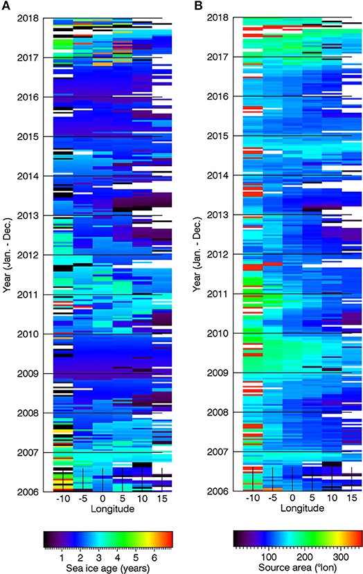
Figure 7. Result of a Lagrangian approach that tracks sea ice backward in time leaving Fram Strait between 81.5°N, 10°W and 15°E (2006–2017, January–December). (A) transit time (age) of sea ice from its formation site to Fram Strait and (B) source area of sea ice exiting Fram Strait (° longitude).

4. Discussion

4.1. Origin of Particles

The particle trajectory experiments showed that particles originate mostly from areas south and southeast of the moorings. They originate mostly from deep areas, with almost no particles originating from shallow areas with depths between 0 and 500 m (Figure 3C). Regarding the simulated catchment areas, this shallow area corresponds to the Svalbard and Barents Sea shelf region. Thus, the strong WSC appears to present a barrier that prevents particles from the shelf to reach central Fram Strait.

However, particles are not only advected by ocean currents, but also carried by sea ice. The ice coverage of the simulated catchment area is not negligible (Figure 5), hence both moorings are located in the marginal ice zone. Hebbeln and Wefer (1991), based on mooring measurements, observed maximum particle fluxes in the marginal ice zone of Fram Strait. The ice tracking analysis revealed that sea ice transported particularly through eastern Fram Strait originates mostly from the Siberian Shelf Seas. Since sea ice formation can occur close to the sea floor in these regions, it can entrain sediments which strongly contribute to particle fluxes in Fram Strait. This is supported by high sea ice melting rates in the Fram Strait marginal ice zone, which results from the interaction with warm AW. Another, indirect way to reveal the origin of particles is the analysis of their composition, e.g., the seasonal and regional variability of clay minerals, as done by Berner and Wefer (1994). In the Fram Strait marginal ice zone / WSC area, the authors found both a high / medium lithogenic content, pointing to the release of ice-rafted material by melting, and koalinite/illite ratios related to high plankton productivity, respectively.

4.2. Seasonality of Particle Catchment Areas

The particle trajectory calculation revealed that the seasonal variation in the particle distribution at the surface is rather low for all 12 experiments (Figure 4 and Figures S1,S2). As shown by observations and model studies, the WSC is stronger in winter than in summer, with higher eddy activity during winter season (Beszczynska-Möller et al., 2012; von Appen et al., 2016; Wekerle et al., 2017). This might lead to a compensating effect, with more particles trapped in eddies despite stronger currents during winter time, overall resulting in a weak seasonal variation of the catchment area.

However, by starting one trajectory calculation per day, we cannot inherently account for differences in particle production rate, which varies considerably during the year. First, the sea ice coverage of the simulated catchment area is highest in summer (the reason for this will be discussed in the next section), and also melting of sea ice is highest during this season. As described above, sea ice can originate from the shallow Siberian shelf seas, carrying sedimentarymaterial that contributes to vertical particle fluxes. Second, the chlorophyll-a concentration of the simulated catchment area reaches its maximum in summer as well ². We suppose that the timing of the maximum bloom is correlated with the highest export efficiency. Although knowing that secondary effects (e.g., ingestion by zooplankton) play a dominant role on particle fluxes, we can expect high particle fluxes measured by the sediment traps in summer and early autumn (depending on the settling velocities, it takes days or even up to months until particles reach the trap). In fact, a sedimentation study conducted in the central Fram Strait during the years 2000–2005 revealed increased vertical particle fluxes in August/September and May/June (Bauerfeind et al., 2009).

4.3. Summer Sea-Ice Maxima of the Simulated Catchment Area

The ice coverage of the simulated catchment areas shows strong seasonal variability (Figure 5). Surprisingly, the highest ice coverage of the catchment area of both HG-N and HG-IV occurs in the summer months, particularly in June. What is the reason for this summer maximum? Tsukernik et al. (2010) showed that anomalies in ice export through Fram Strait can be explained by an east-west dipole pattern of sea level pressure anomaly with centres located over the Barents Sea and Greenland, associated with anomalous meridional winds across Fram Strait. Moreover, Smedsrud et al. (2017) used mean sea level pressure anomalies across Fram Strait to compute geostrophic winds, and a comparison with sea ice drift speed obtained from satellite measurements revealed a high correlation. An almost linear relationship of sea ice export through Fram Strait and wind speed was also shown by Harder et al. (1998) in model experiments. This relationship between sea level pressure and ice export is significant in the winter months, but not in the summer months (Tsukernik et al., 2010). Thus, in the summer, sea ice can move more freely into central Fram Strait (where HG-N and HG-IV are located) and is not as strongly restricted to the western part of Fram Strait as in the winter months. Potentially also the seasonal difference in the strength of the AW recirculation can play a role. The stronger westward flow of AW in winter may inhibit sea ice eastward motion.

4.4. What Is a Realistic Estimate of Settling Velocities?

In our study, we apply a range of constant settling velocities for the trajectory calculation, ranging between 20 and 120 m/d. Settling velocities commonly used in particle trajectory studies range from 50 to 200 m/d (Siegel and Deuser, 1997; Waniek et al., 2000; Siegel et al., 2008; Abell et al., 2013). The choice of values used in this study stems from field measurements conducted in Fram Strait in summer 2016, described in section 2.4. Figure 8 shows settling velocities and associated equivalent spherical diameter measured for in situ collected marine snow at locations HG-IX (close to the Molloy Deep) at 80 m depth and HG-N at 20 m depth. At the Molloy Deep, 22 samples were analyzed, revealing minimum and maximum settling velocities of 5 and 64 m/d, with a mean value of 30 m/d. At location HG-N, the spread of measured values is larger. 7 samples were analyzed, and settling velocities ranged between 2 and 175 m/d, with a mean value of 77 m/d. Particle trajectory experiments conducted in this study with settling velocities of 20 and 60 m/d are thus more realistic than the case with 120 m/d.

FIGURE 8

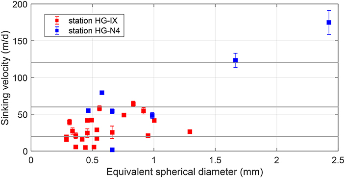
Figure 8. Sinking velocity, its standard deviation and the associated equivalent spherical diameter of aggregates, measured during RV Polarstern expedition PS99.2 in summer 2016 at stations HG-IX (close to the Molloy Deep) in 80 m depth and HG-N4 in 20 m depth. Gray lines indicate settling velocities of 20, 60, and 120 m/d used in this study.

A more realistic approach than using constant settling velocities is the application of the Stokes Law. It relates the particle sinking velocity to the density difference of particle and sea water as well as particle size, as e.g., done in a study by Qiu et al. (2014). However, particle density and size are parameters that are difficult to measure in practice, and furthermore a wide range of particles with different size and density classes occurs in the water column. Processes like fragmentation, aggregation, consumption, and microbial activity can also change the sinking velocity as particles descent through the water column (Siegel et al., 1990). In particular, field observations by Berelson (2001) and Fischer and Karakaş (2009) showed that settling velocities increase with depth. This was explained by carbon loss during degradation in the epi- and mesopelagic which increases particle densities, and by an increase in ballast minerals with depth. Furthermore, the vertical ocean velocity can impact the pathway of the sinking particle. In general, vertical velocities are much smaller than the particle settling velocities used in this study, and are hence neglected. However, vertical velocities associated with sub-mesoscale eddies or filaments can be significantly larger (>50 m/d, von Appen et al., 2018). Moreover, Fram Strait is characterized by a deep mixed layer in the winter months, associated with strong convection events. This also leads to high vertical velocities. To conclude, settling velocities vary with depth, regionally, seasonally and inter-annually. Dedicated studies are required to analyse these processes.

5. Conclusions

In this study we developed a Lagrangian model to determine the catchment area of sediment traps attached to two moorings operated in central Fram Strait. The time-dependent velocity field of a high resolution, eddy resolving sea ice-ocean model was used to compute backward trajectories starting at the trap locations once per day for the time period 2002–2009. Remote sensing products (sea ice concentration and chlorophyll-a distribution) were used to characterize the simulated catchment area.

Our study shows that the extent of the catchment area is larger the deeper the trap and the slower the settling velocity. Particles advected with ocean currents originate mostly from south of the mooring sites, and show a wide spread (45–88% originate from distances larger than 50 km), indicating the influence of the northward flowing WSC, but also of the vigorous eddy field leading to random motion of particles. Particles trapped in mooring HG-N originate from surface areas mostly characterized by Polar Water. In contrast, the simulated catchment area of mooring HG-IV, which is located around 80 km south of HG-N, is mostly characterized by Atlantic Water. For both moorings, particles mostly originate from areas deeper than 500 m, and thus the Svalbard shelf does not play a major role as a source region. Sea ice concentration over the catchment area reaches up to 20%, and is highest in the summer months when the surface air pressure difference between Greenland and Svalbard is low, allowing sea ice to move more freely into central Fram Strait. Thus, particles carried by sea ice could potentially contribute vertical particle fluxes measured by moorings HG-IV and HG-N. A sea ice backtracking method allowed us to determine the source area and age of sea ice advected through Fram Strait. Chlorophyll-a distribution over the simulated catchment area reaches its maximum in June, indicating that highest vertical particle fluxes are expected in the summer months. The catchment areas and integrated remote-sensing products defined in this study will provide a valuable time-series to intepret ongoing changes in pelagic-benthic coupling processes in the Fram Strait.

Data Availability

The backward particle trajectories are available at Pangaea (https://doi.pangaea.de/10.1594/PANGAEA.895078). All datasets used for sea ice tracking are compiled here: http://epic.awi.de/45411/1/AWI_ICETrack_ver2017Sep.pdf. Sea ice concentration data is available at ftp://ftp.ifremer.fr/ifremer/cersat/products/gridded/psi-concentration/data/arctic/daily/netcdf/. Chlorophyll-a data is available at http://marine.copernicus.eu/services-portfolio/access-to-products?option=com_csw&view=details&product_id=OCEANCOLOUR_ARC_CHL_L3_REP_OBSERVATIONS_009_069.

Author Contributions

CW contributed the particle trajectory analysis and wrote most of the manuscript, TK contributed the sea ice tracking and ice coverage analysis, TD contributed the analysis of chlorophyll-a, MI contributed the analysis of measured settling velocities. CW, WJvA, and IS designed this study. All authors discussed the content of the manuscript and contributed to the interpretation of data and writing of the manuscript.

Funding

All authors are funded by the FRontiers in Arctic marine Monitoring program (FRAM).

Conflict of Interest Statement

The authors declare that the research was conducted in the absence of any commercial or financial relationships that could be construed as a potential conflict of interest.

Acknowledgments

Model simulations were performed at the North-German Supercomputing Alliance (HLRN). We would like to thank Ralph Timmermann (AWI) for providing the particle trajectory code. Thanks also to the three reviewers for providing helpful comments on the paper.

Supplementary Material

The Supplementary Material for this article can be found online at: https://www.frontiersin.org/articles/10.3389/fmars.2018.00407/full#supplementary-material

Footnotes

1. ^Since we perform a backtracking particle method, the term “rising speed” would be more appropriate. However, in the literature, the term “sinking velocity” or “settling velocity” is commonly used.

2. ^Note that the satellite measurements cover only the surface layers, a deep chlorophyll-a maximum would not be detected.

References

Abell, R. E., Brand, T., Dale, A. C., Tilstone, G. H., and Beveridge, C. (2013). Variability of particulate flux over the Mid-Atlantic Ridge. Deep Sea Res. II 98, 257–268. doi: 10.1016/j.dsr2.2013.10.005

CrossRef Full Text | Google Scholar

Alldredge, A. L., and Chris, C. G. (1988). In situ settling behavior of marine snow. Limnol. Oceanogr. 33, 339–351. doi: 10.4319/lo.1988.33.3.0339

CrossRef Full Text | Google Scholar

Anderson, T. R., and Ryabchenko, V. A. (2009). Carbon Cycling in the Mesopelagic Zone of the Central Arabian Sea: Results from a Simple Model Washington, DC: American Geophysical Union (AGU), 281–297.

Google Scholar

Antia, A., Koeve, W., Fischer, G., Blanz, T., Schulz-Bull, D., Scholten, J., et al. (2001). Basin-wide particulate carbon flux in the Atlantic Ocean: Regional export patterns and potential for atmospheric CO₂ sequestration. Glob. Biogeochem. Cycles 15, 845–862. doi: 10.1029/2000GB001376

CrossRef Full Text | Google Scholar

Armstrong, R. A., Lee, C., Hedges, J. I., Honjo, S., and Wakeham, S. G. (2001). A new, mechanistic model for organic carbon fluxes in the ocean based on the quantitative association of POC with ballast minerals. Deep Sea Res. II Top. Stud. Oceanogr. 49, 219–236. doi: 10.1016/S0967-0645(01)00101-1

CrossRef Full Text | Google Scholar

Armstrong, R. A., Peterson, M. L., Lee, C., and Wakeham, S. G. (2009). Settling velocity spectra and the ballast ratio hypothesis. Deep Sea Res. II Top. Stud. Oceanogr. 56, 1470–1478. doi: 10.1016/j.dsr2.2008.11.032

CrossRef Full Text | Google Scholar

Asper, V. L., Deuser, W. G., Knauer, G. A., and Lohrenz, S. E. (1992). Rapid coupling of sinking particle fluxes between surface and deep ocean waters. Nature 357, 670–672. doi: 10.1038/357670a0

CrossRef Full Text | Google Scholar

Asper, V. L., and Smith, W. O. (2003). Abundance, distribution and sinking rates of aggregates in the Ross Sea, Antarctica. Deep Sea Res. I 50, 131–150. doi: 10.1016/S0967-0637(02)00146-2

CrossRef Full Text | Google Scholar

Bauerfeind, E., Nöthig, E.-M., Beszczynska, A., Fahl, K., Kaleschke, L., Kreker, K., et al. (2009). Particle sedimentation patterns in the eastern Fram Strait during 2000-2005: Results from the Arctic long-term observatory HAUSGARTEN. Deep Sea Res. I 56, 1471–1487. doi: 10.1016/j.dsr.2009.04.011

CrossRef Full Text | Google Scholar

Berelson, W. M. (2001). Particle settling rates increase with depth in the ocean. Deep Sea Res. II 49, 237–251. doi: 10.1016/S0967-0645(01)00102-3

CrossRef Full Text | Google Scholar

Berner, H., and Wefer, G. (1994). Clay-mineral flux in the fram strait and Norwegian sea. Mar. Geol. 116, 327–345. doi: 10.1016/0025-3227(94)90049-3

CrossRef Full Text | Google Scholar

Beszczynska-Möller, A., Fahrbach, E., Schauer, U., and Hansen, E. (2012). Variability in Atlantic water temperature and transport at the entrance to the Arctic Ocean, 1997–2010. ICES J. Mar. Sci. 69, 852–863. doi: 10.1093/icesjms/fss056

CrossRef Full Text | Google Scholar

Billett, D. S. M., Lampitt, R. S., Rice, A. L., and Mantoura, R. F. C. (1983). Seasonal sedimentation of phytoplankton to the deep-sea benthos. Nature 302, 520–522. doi: 10.1038/302520a0

CrossRef Full Text | Google Scholar

Burd, A. B., Hansell, D. A., Steinberg, D. K., Anderson, T. R., Aristegui, J., Baltar, F., et al. (2010). Assessing the apparent imbalance between geochemical and biochemical indicators of meso- and bathypelagic biological activity: What the @$#! is wrong with present calculations of carbon budgets? Deep Sea Res. II Top. Stud. Oceanogr. 57, 1557–1571. doi: 10.1016/j.dsr2.2010.02.022

CrossRef Full Text | Google Scholar

Cherkasheva, A., Bracher, A., Melsheimer, C., Köberle, C., Gerdes, R., Nöthig, E.-M., et al. (2014). Influence of the physical environment on polar phytoplankton blooms: a case study in the Fram Strait. J. Mar. Syst. 132, 196–207. doi: 10.1016/j.jmarsys.2013.11.008

CrossRef Full Text | Google Scholar

Dai, A., Qian, T., Trenberth, K. E., and Milliman, J. D. (2009). Changes in Continental Freshwater Discharge from 1948 to 2004. J. Climate 22, 2773–2792. doi: 10.1175/2008JCLI2592.1

CrossRef Full Text | Google Scholar

Damm, E., Bauch, D., Krumpen, T., Rabe, B., Korhonen, M., Vinogradova, E., et al. (2018). The transpolar drift Conveys methane from the siberian shelf to the central Arctic ocean. Sci. Rep. 8, 1–10. doi: 10.1038/s41598-018-22801-z

PubMed Abstract | CrossRef Full Text | Google Scholar

Danilov, S., Wang, Q., Timmermann, R., Iakovlev, N., Sidorenko, D., Kimmritz, M., et al. (2015). Finite-Element Sea Ice Model (FESIM), version 2. Geosci. Model Dev. 8, 1747–1761. doi: 10.5194/gmd-8-1747-2015

CrossRef Full Text | Google Scholar

de Steur, L., Hansen, E., Gerdes, R., Karcher, M., Fahrbach, E., and Holfort, J. (2009). Freshwater fluxes in the East Greenland Current: a decade of observations. Geophys. Res. Lett. 36, 1–5. doi: 10.1029/2009GL041278

CrossRef Full Text | Google Scholar

Dethleff, D., and Kempema, E. (2007). Langmuir circulation driving sediment entrainment into newly formed ice: tank experiment results with application to nature (Lake Hattie, United States; Kara Sea, Siberia). J. Geophys. Res. Oceans 112, 1–15. doi: 10.1029/2005JC003259

CrossRef Full Text | Google Scholar

Deuser, W. G., Muller-Karger, F. E., and Hemleben, C. (1988). Temporal variations of particle fluxes in the deep subtropical and tropical North Atlantic: eulerian versus lagrangian effects. J. Geophys. Res. Oceans 93, 6857–6862. doi: 10.1029/JC093iC06p06857

CrossRef Full Text | Google Scholar

Deuser, W. G., and Ross, E. H. (1980). Seasonal change in the flux of organic carbon to the deep Sargasso Sea. Nature 283, 364–365. doi: 10.1038/283364a0

CrossRef Full Text | Google Scholar

Döös, K., Jönsson, B., and Kjellsson, J. (2017). Evaluation of oceanic and atmospheric trajectory schemes in the TRACMASS trajectory model v6.0. Geosci. Model Dev. 10, 1733–1749. doi: 10.5194/gmd-10-1733-2017

CrossRef Full Text | Google Scholar

Döös, K., Rupolo, V., and Brodeau, L. (2011). Dispersion of surface drifters and model-simulated trajectories. Ocean Model. 39, 301–310. doi: 10.1016/j.ocemod.2011.05.005

CrossRef Full Text | Google Scholar

Durkin, C. A., Estapa, M. L., and Buesseler, K. O. (2015). Observations of carbon export by small sinking particles in the upper mesopelagic. Mar. Chem. 175, 72–81. doi: 10.1016/j.marchem.2015.02.011

CrossRef Full Text | Google Scholar

Eicken, H., Kolatschek, J., Freitag, J., Lindemann, F., Kassens, H., and Dmitrenko, I. (2000). A key source area and constraints on entrainment for basin–scale sediment transport by Arctic sea ice. Geophys. Res. Lett. 27, 1919–1922. doi: 10.1029/1999GL011132

CrossRef Full Text | Google Scholar

Ezraty, R., Girard-Ardhuin, F., Piolle, J. F., Kaleschke, L., and Heygster, G. (2007). Arctic and Antarctic Sea Ice Concentration and Arctic Sea Ice Drift Estimated from Special Sensor Microwave Data, 2.1 Edn. Technical report, Departement d'Oceanographie Physique et Spatiale, IFREMER, Brest, France and University of Bremen.

Google Scholar

Fischer, G., and Karakaş, G. (2009). Sinking rates and ballast composition of particles in the Atlantic Ocean: implications for the organic carbon fluxes to the deep ocean. Biogeosciences 6, 85–102. doi: 10.5194/bg-6-85-2009

CrossRef Full Text | Google Scholar

Gohin, F., Saulquin, B., Oger-Jeanneret, H., Lozac'h, L., Lampert, L., Lefebvre, A., et al. (2008). Towards a better assessment of the ecological status of coastal waters using satellite-derived chlorophyll-a concentrations. Remote Sens. Environ. 112, 3329–3340. doi: 10.1016/j.rse.2008.02.014

CrossRef Full Text | Google Scholar

Graf, G. (1998). Benthic-pelagic coupling in a deep-sea benthic community. Nature 341, 437–439. doi: 10.1038/341437a0

CrossRef Full Text | Google Scholar

Harder, M., Lemke, P., and Hilmer, M. (1998). Simulation of sea ice transport through Fram Strait: natural variability and sensitivity to forcing. J. Geophys. Res. Oceans 103, 5595–5606. doi: 10.1029/97JC02472

CrossRef Full Text | Google Scholar

Hebbeln, D., and Wefer, G. (1991). Effects of ice coverage and ice-rafted material on sedimentation in the Fram Strait. Nature 350, 409–411. doi: 10.1038/350409a0

CrossRef Full Text | Google Scholar

Heinze, C., and Maier-Reimer, E. (1991). Glacial CO₂ reduction by the world ocean: experiments with the Hamburg carbon cycle model. Paleoceanography 6, 395–430. doi: 10.1029/91PA00489

CrossRef Full Text | Google Scholar

Hu, C., Lee, Z., and Franz, B. (2012). Chlorophyll a algorithms for oligotrophic oceans: a novel approach based on three-band reflectance difference. J. Geophys. Res. Oceans 117, 1–25. doi: 10.1029/2011JC007395

CrossRef Full Text | Google Scholar

Ittekkot, V. (1993). The abiotically driven biological pump in the ocean and short-term fluctuations in atmospheric CO₂ contents. Glob. Planet. Change 8, 17–25. doi: 10.1016/0921-8181(93)90060-2

CrossRef Full Text | Google Scholar

Iversen, M. H., and Ploug, H. (2010). Ballast minerals and the sinking carbon flux in the ocean: carbon-specific respiration rates and sinking velocity of marine snow aggregates. Biogeosciences 7, 2613–2624. doi: 10.5194/bg-7-2613-2010

CrossRef Full Text | Google Scholar

Jiao, N., Herndl, G. J., Hansell, D. A., Benner, R., Kattner, G., Wilhelm, S. W., et al. (2010). Microbial production of recalcitrant dissolved organic matter: long-term carbon storage in the global ocean. Nat. Rev. Microbiol. 8, 593–599. doi: 10.1038/nrmicro2386

PubMed Abstract | CrossRef Full Text | Google Scholar

Jónasdóttir, S. H., Visser, A. W., Richardson, K., and Heath, M. R. (2015). Seasonal copepod lipid pump promotes carbon sequestration in the deep North Atlantic. Proc. Natl. Acad. Sci. U.S.A. 112, 12122–12126. doi: 10.1073/pnas.1512110112

PubMed Abstract | CrossRef Full Text | Google Scholar

Klaas, C., and Archer, D. E. (2002). Association of sinking organic matter with various types of mineral ballast in the deep sea: Implications for the rain ratio. Glob. Biogeochem. Cycles 16, 63–1–63–14. doi: 10.1029/2001GB001765

CrossRef Full Text | Google Scholar

Krumpen, T., Gerdes, R., Haas, C., Hendricks, S., Herber, A., Selyuzhenok, V., et al. (2016). Recent summer sea ice thickness surveys in fram Strait and associated ice volume fluxes. Cryosphere 10, 523–534. doi: 10.5194/tc-10-523-2016

CrossRef Full Text | Google Scholar

Kwon, E. Y., Primeau, F., and Sarmiento, J. L. (2009). The impact of remineralization depth on the air-sea carbon balance. Nat. Geosci. 2, 630–635. doi: 10.1038/ngeo612

CrossRef Full Text | Google Scholar

Large, W., and Yeager, S. (2008). The global climatology of an interannually varying air-sea flux data set. Clim. Dynam. 33, 341–364. doi: 10.1007/s00382-008-0441-3

CrossRef Full Text | Google Scholar

Lombard, F., Guidi, L., and Kiørboe, T. (2013). Effect of type and concentration of ballasting particles on sinking rate of marine snow produced by the appendicularian oikopleura dioica. PLoS ONE 8:e75676. doi: 10.1371/journal.pone.0075676

PubMed Abstract | CrossRef Full Text | Google Scholar

McDonnell, A. M. P., and Buesseler, K. O. (2010). Variability in the average sinking velocity of marine particles. Limnol. Oceanogr. 55, 2085–2096. doi: 10.4319/lo.2010.55.5.2085

CrossRef Full Text | Google Scholar

Nöthig, E.-M., Bracher, A., Engel, A., Metfies, K., Niehoff, B., Peeken, I., et al. (2015). Summertime plankton ecology in Fram Strait–a compilation of long- and short-term observations. Polar Res. 34:23349. doi: 10.3402/polar.v34.23349

CrossRef Full Text | Google Scholar

Peeken, I., Primpke, S., Beyer, B., Gütermann, J., Katlein, C., Krumpen, T., et al. (2018). Arctic sea ice is an important temporal sink and means of transport for microplastic. Nat. Commun. 9, 1505. doi: 10.1038/s41467-018-03825-5

PubMed Abstract | CrossRef Full Text | Google Scholar

Peterson, M. L., Wakeham, S. G., Lee, C., Askea, M. A., and Miquel, J. C. (2005). Novel techniques for collection of sinking particles in the ocean and determining their settling rates. Limnol. Oceanogr. Methods 3, 520–532. doi: 10.4319/lom.2005.3.520

CrossRef Full Text | Google Scholar

Ploug, H., Terbrüggen, A., Kaufmann, A., Wolf-Gladrow, D., and Passow, U. (2010). A novel method to measure particle sinking velocity in vitro, and its comparison to three other in vitro methods. Limnol. Oceanogr. Methods 8, 386–393. doi: 10.4319/lom.2010.8.386

CrossRef Full Text | Google Scholar

Qiu, Z., Doglioli, A. M., and Carlotti, F. (2014). Using a Lagrangian model to estimate source regions of particles in sediment traps. Sci. China Earth Sci. 57, 2447–2456. doi: 10.1007/s11430-014-4880-x

CrossRef Full Text | Google Scholar

Rembauville, M., Blain, S., Manno, C., Tarling, G., Thompson, A., Wolff, G., et al. (2018). The role of diatom resting spores in pelagic–benthic coupling in the Southern Ocean. Biogeosciences 15, 3071–3084. doi: 10.5194/bg-15-3071-2018

CrossRef Full Text | Google Scholar

Riley, J. S., Sanders, R., Marsay, C., Moigne, F. A. C. L., Achterberg, E. P., and Poulton, A. J. (2012). The relative contribution of fast and slow sinking particles to ocean carbon export. Glob. Biogeochem. Cycles 26, 1–10. doi: 10.1029/2011GB004085

CrossRef Full Text | Google Scholar

Sabine, C. L., Feely, R. A., Gruber, N., Key, R. M., Lee, K., Bullister, J. L., et al. (2004). The oceanic sink for anthropogenic CO₂. Science 305, 367–371. doi: 10.1126/science.1097403

PubMed Abstract | CrossRef Full Text | Google Scholar

Salter, I., Kemp, A. E. S., Lampitt, R. S., and Gledhill, M. (2010). The association between biogenic and inorganic minerals and the amino acid composition of settling particles. Limnol. Oceanogr. 55, 2207–2218. doi: 10.4319/lo.2010.55.5.2207

CrossRef Full Text | Google Scholar

Salter, I., Schiebel, R., Ziveri, P., Movellan, A., Lampitt, R., and Wolff, G. A. (2014). Carbonate counter pump stimulated by natural iron fertilization in the Polar Frontal Zone. Nat. Geosci. 7, 885–889. doi: 10.1038/ngeo2285

CrossRef Full Text | Google Scholar

Sarmiento, J. L., and Gruber, N. (2006). Ocean Biogeochemical Dynamics. Princeton, NJ: Princeton University Press.

Google Scholar

Sarmiento, J. L., Herbert, T. D., and Toggweiler, J. R. (1988). Causes of anoxia in the world ocean. Glob. Biogeochem. Cycles 2, 115–128. doi: 10.1029/GB002i002p00115

CrossRef Full Text | Google Scholar

Sarmiento, J. L., and Toggweiler, J. R. (1984). A new model for the role of the oceans in determining atmospheric PCO₂. Nature 308, 621–624. doi: 10.1038/308621a0

CrossRef Full Text | Google Scholar

Siegel, D., and Deuser, W. (1997). Trajectories of sinking particles in the Sargasso Sea: modeling of statistical funnels above deep-ocean sediment traps. Deep Sea Res. I 44, 1519–1541. doi: 10.1016/S0967-0637(97)00028-9

CrossRef Full Text | Google Scholar

Siegel, D., Fields, E., and Buesseler, K. (2008). A bottom-up view of the biological pump: Modeling source funnels above ocean sediment traps. Deep Sea Res. I 55, 108–127. doi: 10.1016/j.dsr.2007.10.006

CrossRef Full Text | Google Scholar

Siegel, D., Granata, T. C., Michaels, A. F., and Dickey, T. D. (1990). Mesoscale eddy diffusion, particle sinking, and the interpretation of sediment trap data. J. Geophys. Res. Oceans 95, 5305–5311. doi: 10.1029/JC095iC04p05305

CrossRef Full Text | Google Scholar

Smedsrud, L. H., Halvorsen, M. H., Stroeve, J. C., Zhang, R., and Kloster, K. (2017). Fram Strait sea ice export variability and September Arctic sea ice extent over the last 80 years. Cryosphere 11, 65–79. doi: 10.5194/tc-11-65-2017

CrossRef Full Text | Google Scholar

Soltwedel, T., Schauer, U., Boebel, O., Nothig, E., Bracher, A., Metfies, K., et al. (2013). “FRAM-FRontiers in Arctic marine Monitoring: visions for permanent observations in a gateway to the Arctic Ocean,” in 2013 MTS/IEEE OCEANS (Bergen).

Google Scholar

Timmermann, R., Danilov, S., Schröter, J., Böning, C., Sidorenko, D., and Rollenhagen, K. (2009). Ocean circulation and sea ice distribution in a finite element global sea ice-ocean model. Ocean Model. 27, 114–129. doi: 10.1016/j.ocemod.2008.10.009

CrossRef Full Text | Google Scholar

Trull, T., Bray, S., Buesseler, K., Lamborg, C., Manganini, S., Moy, C., et al. (2008). In situ measurement of mesopelagic particle sinking rates and the control of carbon transfer to the ocean interior during the Vertical Flux in the Global Ocean (VERTIGO) voyages in the North Pacific. Deep Sea Res. II Top. Stud. Oceanogr. 55, 1684–1695. doi: 10.1016/j.dsr2.2008.04.021

CrossRef Full Text | Google Scholar

Tsukernik, M., Deser, C., Alexander, M., and Tomas, R. (2010). Atmospheric forcing of Fram Strait sea ice export: a closer look. Climate Dyn. 35, 1349–1360. doi: 10.1007/s00382-009-0647-z

CrossRef Full Text | Google Scholar

Turner, C. R., Barnes, M. A., Xu, C. C., Jones, S. E., Jerde, C. L., and Lodge, D. M. (2014). Particle size distribution and optimal capture of aqueous macrobial eDNA. Methods Ecol. Evolut. 5, 676–684. doi: 10.1111/2041-210X.12206

CrossRef Full Text | Google Scholar

Turner, J. T. (2002). Zooplankton fecal pellets, marine snow and sinking phytoplankton blooms. Aquat. Microb. Ecol. 27, 57–102. doi: 10.3354/ame027057

CrossRef Full Text | Google Scholar

v. Gyldenfeldt, A.-B., Carstens, J., and Meincke, J. (2000). Estimation of the catchment area of a sediment trap by means of current meters and foraminiferal tests. Deep Sea Res. II 47, 1701–1717. doi: 10.1016/S0967-0645(00)00004-7

CrossRef Full Text | Google Scholar

Volk, T., and Hoffert, M. (1985). Ocean Carbon Pumps: analysis of relative strengths and efficiencies in ocean-driven atmospheric CO₂ changes, Am. Geophys. Union Geophys. Monogr. 32. 99–110. doi: 10.1029/GM032p0099

CrossRef Full Text | Google Scholar

von Appen, W.-J., Schauer, U., Hattermann, T., and Beszczynska-Möller, A. (2016). Seasonal cycle of mesoscale instability of the West Spitsbergen current. J. Phys. Oceanogr. 46, 1231–1254. doi: 10.1175/JPO-D-15-0184.1

CrossRef Full Text | Google Scholar

von Appen, W.-J., Wekerle, C., Hehemann, L., Schourup-Kristensen, V., Konrad, C., and Iversen, M. H. (2018). Observations of a submesoscale cyclonic filament in the marginal ice zone. Geophys. Res. Lett. 45, 6141–6149. doi: 10.1029/2018GL077897

CrossRef Full Text | Google Scholar

Waite, A. M., Stemmann, L., Guidi, L., Calil, P. H. R., Hogg, A. M. C., Feng, M., et al. (2016). The wineglass effect shapes particle export to the deep ocean in mesoscale eddies. Geophys. Res. Lett. 43, 9791–9800. doi: 10.1002/2015GL066463

CrossRef Full Text | Google Scholar

Wang, Q., Danilov, S., Sidorenko, D., Timmermann, R., Wekerle, C., Wang, X., et al. (2014). The Finite Element Sea Ice-Ocean Model (FESOM) v.1.4: formulation of an ocean general circulation model. Geosci. Model Dev. 7, 663–693. doi: 10.5194/gmd-7-663-2014

CrossRef Full Text | Google Scholar

Waniek, J., Koeve, W., and Prien, R. D. (2000). Trajectories of sinking particles and the catchment areas above sediment traps in the northeast Atlantic. J. Mar. Res. 58, 983–1006. doi: 10.1357/002224000763485773

CrossRef Full Text | Google Scholar

Waniek, J. J., Schulz-Bull, D. E., Blanz, T., Prien, R. D., Oschlies, A., and Müller, T. J. (2005). Interannual variability of deep water particle flux in relation to production and lateral sources in the northeast Atlantic. Deep Sea Res. I Oceanogr. Res. Pap. 52, 33–50. doi: 10.1016/j.dsr.2004.08.008c

CrossRef Full Text | Google Scholar

Wegner, C., Wittbrodt, K., Hölemann, J., Janout, M., Krumpen, T., Selyuzhenok, V., et al. (2017). Sediment entrainment into sea ice and transport in the Transpolar Drift: a case study from the Laptev Sea in winter 2011/2012. Cont. Shelf Res. 141, 1–10. doi: 10.1016/j.csr.2017.04.010

CrossRef Full Text | Google Scholar

Wekerle, C., Wang, Q., von Appen, W.-J., Danilov, S., Schourup-Kristensen, V., and Jung, T. (2017). Eddy-Resolving Simulation of the Atlantic Water Circulation in the Fram Strait With Focus on the Seasonal Cycle. J. Geophys. Res. Oceans 122, 8385–8405. doi: 10.1002/2017JC012974

CrossRef Full Text | Google Scholar

Zeebe, R. E. (2012). History of seawater carbonate chemistry, atmospheric CO₂, and Ocean Acidification. Ann. Rev. Earth Planet. Sci. 40, 141–165. doi: 10.1146/annurev-earth-042711-105521

CrossRef Full Text | Google Scholar

Appendix: Particle Tracking Algorithm

The Lagrangian particle-tracking algorithm is based on the following equation:

$\begin{array}{ll}\frac{d\text{x}}{dt}=\text{u}(\text{x},t),& (1)\end{array}$

where x is the 3D particle position and u is the 3D velocity field at the particle position. If we knew the particle position at time n, the position at time n + 1 will be

$\begin{array}{ll}\text{x}(t_{n+1})=\text{x}(t_n)+{\displaystyle {\int }_{t_n}^{t_{n+1}}}\text{u}(\text{x},t)dt.& (2)\end{array}$

We use the Euler method to compute the particle position at time t_n+1 = t_n + δt:

$\begin{array}{ll}\text{x}(t_{n+1})=\text{x}(t_n)+\text{u}(\text{x}(t_n),t_n)\delta t.& (3)\end{array}$