Corrigendum: Toward High-Resolution Vertical Measurements of Dissolved Greenhouse Gases (Nitrous Oxide and Methane) and Nutrients in the Eastern South Pacific
 Macarena Troncoso
 Gerardo Garcia
 Josefa Verdugo
 Laura Farías
- 1Programa de Postgrado en Oceanografía, Departamento de Oceanografía, Universidad de Concepción, Concepción, Chile
- 2Laboratorio de Biogeoquímica Isotópica, Departamento de Oceanografía, Universidad de Concepción, Concepción, Chile
- 3Centro de Ciencia del Clima y la Resiliencia (CR)2, Universidad de Concepción, Concepción, Chile
- 4Alfred-Wegener-Institute Helmholtz-Centre for Polar and Marine Research, Bremerhaven, Germany
In this study, in situ, real-time and high-resolution vertical measurements of dissolved greenhouse gases (GHGs) such as nitrous oxide (N2O) and methane (CH4) and nutrients are reported for the eastern South Pacific (ESP); a region with marked zonal gradients, ranging from highly productive and suboxic conditions in coastal upwelling systems to oligotrophic and oxygenated conditions in the subtropical gyre. Four high-resolution vertical profiles for gases (N2O and CH4) and nutrients ( and ) were measured using a Pumped Profiling System (PPS), connected with a liquid degassing membrane coupled with Cavity Ring-Down Spectroscopy (CRDS) and a nutrient auto-analyzer, respectively. The membrane-CRDS system maintains a linear response over a wide range of gas concentrations, detecting N2O and CH4 levels as low as 0.0774 ± 0.0004 and 0.1011 ± 0.001 ppm, respectively. Continuous profiles for gases and nutrients were similar to those reported throughout the ESP, with pronounced N2O and CH4 peaks at the upper oxycline and at the base of the euphotic zone and pycnocline, respectively, in the coastal zone; but almost constant depth profiles in the subtropical gyre. Additionally, other vertical gas and nutrient structures were observed using continuous sampling, which would not have been detected by discrete sampling. Our results demonstrate that continuous measurements can be a potentially useful methodology for future GHGs cycle studies.
Introduction
Dissolved gas analysis involves headspace, purge and tramp, microextraction, and stripping techniques which separate dissolved gases from a liquid matrix and use specialized instruments to measure their concentrations (Jones and Schuberth, 1989; Snow and Slack, 2002; Stashenko and Martínez, 2010; Magen et al., 2014). Gas chromatography (GC) is the most frequently used technique, due to its accuracy of gas measurements such as methane (CH4) and nitrous oxide (N2O). Given the importance of these greenhouse gases (GHGs) to current climate change research, scientific instruments and measurement accuracy have notably improved over the past decades. Technology developments include Membrane Inlet Mass Spectrometry (MIMS), purge-and-trap GC-MS systems (Andrews et al., 2015) and Cavity Ring Down Spectroscopy (CRDS). The latter is a highly sensitive and reproducible technology of direct absorption spectroscopy, which determines nanomolar levels of CH4 and N2O (Crosson, 2008; Berden and Engeln, 2009; Warner et al., 2013; Roberts and Shiller, 2015; Yver Kwok et al., 2015). Despite a substantial increase in the number of GHGs measurements using CRDS, primarily due to improvements in commercially available instruments (i.e., from Los Gatos Research and PICARRO Ltd.), there is an urgent need to improve gas separation techniques.
Currently, most GHGs measurements from seawater are based on the collection of discrete water samples over a range of depths and on-board seawater equilibration analysis (Johnson, 1999). However, some progress has been made for continuous ongoing measurements in the field, using an equilibrator connected to CRDS for N2O and CH4 (Arevalo-Martinez et al., 2013; Grefe and Kaiser, 2014; O'Reilly et al., 2015; Roberts and Shiller, 2015; Brannon et al., 2016; Kock et al., 2016). Recently, polydimethylsiloxane membranes (PDMS) (Helixmark, Carpinteria, CA, USA), coupled with MIMS and CDRS, have shown promising advances for GHGs measurements in freshwater (Bell et al., 2007; Gonzalez-Valencia et al., 2014).
Global GHGs distribution in the ocean is spatially and vertically heterogeneous, with marine regions acting either as a GHGs source or sink, due to biogeochemical (microbial) and physical (mixing and stratification) processes (Bates et al., 1996; Reeburgh, 2007). Spatial and vertical distributions of N2O and CH4 are driven primarily by trophic conditions (organic matter availability) and dissolved O2 levels (Bange et al., 2010; Naqvi et al., 2010). These conditions can be highly variable in the ESP, where coastal upwelling with high biomass accumulation and the presence of an oxygen minimum zone (OMZ) play a key role controlling biogeochemical processes involved in N2O and CH4 cycle (Charpentier et al., 2010; Naqvi et al., 2010). In contrast to coastal zones, the subtropical gyre presents significantly higher oxygen levels, undetectable nutrient concentrations and Chlorophyll-a (Chl-a) values as low as 0.017 mg m−3 (Ras et al., 2008; Lepère et al., 2009). These contrasting environments require more detailed study, particularly for small-scale vertical variations in pycnoclines and oxyclines.
Despite the fact that vertical nutrient gradients and small-scale transport processes are up to two orders of magnitude faster and more intense than those observed over a horizontal scale (Denman and Gargett, 1995), there is a lack of high-resolution vertical measurements of dissolved gases and nutrients in the ocean. This study applies a novel methodology to provide further insights into high-resolution vertical profiles for N2O, CH4, , and throughout the water column.
Materials and Methods
Sampling
Sampling was carried out during two cruises onboard the Chilean R.V. Cabo de Hornos: the CIMAR21 cruise between Caldera (70°52′W−−27°00′S) and Easter Island (109°20′W−27°10′S) from October 11th to November 11th, 2015; and the LowPhox I cruise between Iquique (70°12′W–20°05′S) and Coquimbo (71°36′W−29°29′S) from November 27th to December 9th, 2015 (Figure 1). In this study, four stations were selected, located in contrasting environments. Continuous and discrete samplings were carried out to compare both methodologies.
FIGURE 1
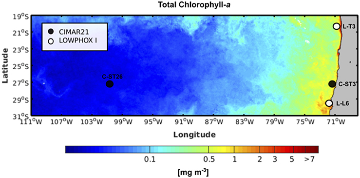
Figure 1. Study area showing the location of sampling stations superimposed on an image illustrating mean surface Chl-a concentrations during the austral spring period (Color data is available at https://modis.gsfc.nasa.gov/data/dataprod/chlor_a.php), Chl-a concentration is expressed in mg Chl-a m−3 (coded according to the color bar); Cruise tracks are shown. CIMAR21 cruise included 24 stations (black dots, sampled stations) covering a zonal distance of about 3,750 km with depths exceeding 1,500 m, while LOWPHOX I cruise sampled 12 stations (white dots, sampled stations) covering a latitudinal distance of about 1,000 km with depths up to 3,000 m.
Continuous Sampling for Gases and Nutrients
Continuous GHGs measurements were carried out using PICARRO G-2308 for CRDS 1 To obtain high-resolution profiles for gases (N2O and CH4 at <1 m depth intervals) and nutrients ( and at 5 m depth intervals), seawater was collected with a Pumped Profiling System (PPS) associated in real-time to a Sea-Bird 25 CTD (conductivity-temperature-depth). Continuous measurements of temperature, conductivity, O2, fluorescence and PAR were taken by additional sensors on the CTD (Bellevue, WA, USA) (see Supplementary Table 1). In addition, online analyses were carried out for gas and nutrient samples during PPS downcast pumping, to ensure continuous velocity control. The pumping mechanism was previously used by De Brabandere et al. (2014). The PPS outlet was directly connected to a PermSelect® PDMSXA-2500 liquid degassing membrane in order to facilitate the extraction and separation of gases from seawater. Membrane characteristics and their physical features are included in Table 1. The membrane had two outlets: one for gases (to flow through to the CRDS) and another one for degassed seawater. For the correct use of the degassing membrane, a maximum flow of 0.5 mL L−1 was maintained, and room temperature and pressure were considered to estimate the permeability of each gas. The gas-permeable silicone membrane with a 2,500 cm2 surface area facilitates gas transfer through the differences in partial pressure between the inside and the outside of the membrane (see permselect.com/markets/degassing). The membrane is composed of 3,200 hollow polydimethylsiloxane fibers (PDMS) of 190 μm internal diameter and 55 μm thickness. The unit containing the silicone membrane has an inlet port for the entry of liquid samples, which then flow through a collecting pipe. Gases with higher permeability are transferred at a higher rate through membrane walls, leaving behind less permeable gases. A zero grade Airgas UZ300C (sweep gas) was injected at 200 mL min−1 in order to carry permeate (transferre) gases to the unit output, which was connected to the input of PICARRO G-2308. The permeability coefficient (Perm) was used to calculate permeated gas flow (Q) through the PermSelect membrane for N2O and CH4 (Table 1), using the following equation:
Q = Permeated gas flow in cm3 s−1
Perm = Permeability Coefficient [0.10–10 cm3·cm/(cm2·s·cm-Hg)]
Pg = Partial gas pressure in cm-Hg
A = Membrane Module Area in cm2
t = Silicone Membrane Wall Thickness (50 cm·10−4)
TABLE 1
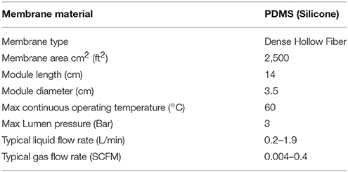
Table 1. Characteristics and operating conditions of PDMX-2500 membrane.
Another important feature of inorganic membranes is the gas separation factor. The latter must be equal to or >5, and it is assumed that each gas flows independently through the membrane, unaffected by the presence of other gases. In this case, the ratio between permeability fluxes was calculated and the separation factor between N2O and CH4 gas was >5, therefore allowing simultaneous measurements.
The PPS operated at a rate of 2.7 L min−1 with a pump-to-deck time of 270 s, ensuring minimum manipulation and avoiding contamination by oxygen and other gases (De Brabandere et al., 2014). In situ temperature was recorded as water passed through the PPS and used for gas solubility calculations. PPS was also connected to a nutrient autoanalyzer for and measurements (see Figure 2).
FIGURE 2
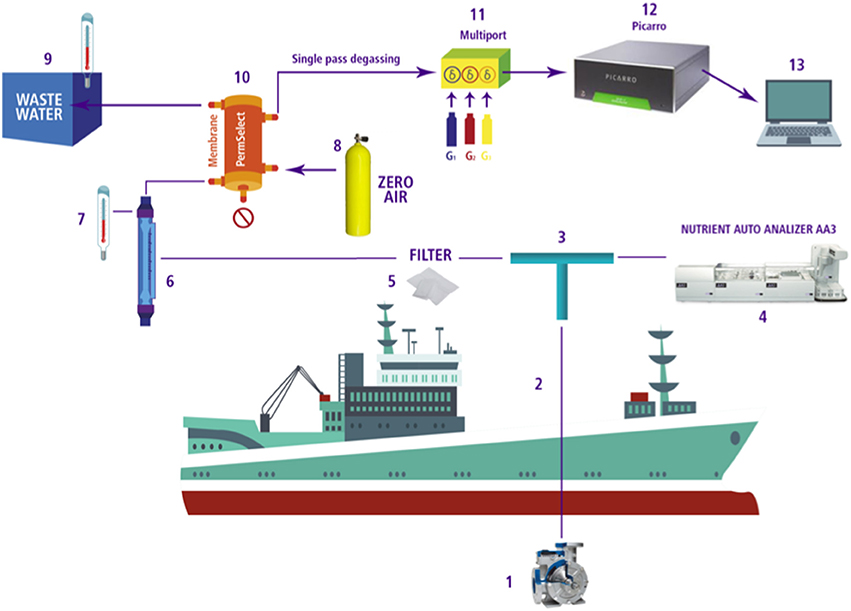
Figure 2. Diagram of continuous gas and nutrient measurement system coupled with the PPS used during the CIMAR21 and Lowphox I cruises. Each phase is delineated as follows: 1. Pumped Profiling System (PPS); 2. Nylon tubing; 3. T -shaped connection; 4. Nutrient AutoAnalyzer (Seal Analytical AA3); 5. 200 micron water filter; 6. Water flow meter; 7. Temperature measurement; 8. Zero air gas as carrier; 9. Waste water with temperature measurement; 10. Degassing membrane (Permeselect-2500); 11. Multiport and standard gases; 12. PI CARRO G-2308 spectrometer; 13. Obtaining data and monitoring.
Extraction and Separation of Gases in Continuous Pumping
The transport mechanism for mass transfer across non-porous membranes is best described by the solution–diffusion model, according to Fick's second law. Mass flux (F) across the membrane is given by:
where D is the diffusion coefficient of the specific compound through the membrane; A is the area across which diffusion takes place, d is membrane thickness, Cm,out is outer membrane concentration (gas side), Cm,in is the inner membrane concentration (feed side) where liquid phase molecules are in contact with the membrane, Kp is the membrane-gas distribution coefficient, and Cg,out and Cg,in are the gas concentrations outside and inside of the membrane, respectively (Boutsiadou, 2012; Gonzalez-Valencia et al., 2014).
Membrane concentrations (Cm) are related to gas phase concentrations based on the Kp gas membrane distribution coefficient, as follows:
where Kd is the membrane-water partition coefficient and H is the Henry's coefficient given by the following equations:
where Cw is the dissolved gas concentration in the water sample (N2O or CH4) and Cg is the gas concentration in the headspace measured as an equilibrium between phases, and:
Seawater was pumped by the PPS at a constant speed of 0.0409 ms−1, using a 0.735″ diameter Nylon hose covered with a layer of PTFE Tape and KEVLAR braid to improve thermo properties. The degassing membrane was connected to the seawater inlet at constant flow and to another inlet with a gas carrier (zero air). The maximum recommended trans-membrane pressure (TMP) for the lateral liquid flow of the envelope is 15 psi (http://permselect.com/markets/liquid_gassing). The water flow from the PPS to the degassing membrane (PermSelect 2500)2 was kept at 0.5 mL L−1 by a flowmeter. Room temperature and pressure were also monitored.
As shown in Figure 2, seawater enters the central port of the membrane contactor, flows through the exterior of the hollow fibers, and exits through the side ports. As water flows through the hollow fiber bundle, dissolved gases are driven by the vacuum generated by the PPS and penetrate the walls of the hollow fibers. Extracted gases flow into the CRDS analyzer and degassed liquid exits through the membrane's side orifices. CRDS reported N2O and CH4 concentrations every 0.05 m, with n = 30 measurements per meter. Considering variations between the two sampling zones (eutrophic and oligotrophic), a cleaning protocol for the degassing membrane was applied, switching from an alkaline cycle with 2–5% NaOH w/w to a citric acid cycle at 5.2% w/w at 50°C for 30 min. Membranes were tested in fresh and seawater, finding non-significant differences between materials (data not shown).
Calibration
A set of gas standards was used in order to calibrate the CRDS and membrane connected to CRDS or M-CRDS (Table 3). Standards included those provided by NOAA to the SCOR working group #143. Calibration was first performed using standards for gases injected directly into the sample module with airtight TEDLAR bags to avoid contamination and pressure interference. Gas separation efficiency for the degassing membrane was tested using seawater equilibrated with the gas phase of known N2O and CH4 levels (gas standards), and then measured using M-CRDS. In order to perform different lab tests, dissolved gases were measured using membrane-CRDS and GC. In order to carry out this process, GC vials (1 L) were filled with atmospherically equilibrated aged seawater and hermetically sealed. Seawater was then replaced with 250 mL of different gas standards (Table 3), creating a headspace and allowing equilibration of both phases. Thus, expected dissolved gas concentrations were estimated at room temperature (where bottles were equilibrated) and salinity of the sample using Henry's law constant. In parallel, dissolved gases in the seawater were measured using M-CRDS system.
Analytical Gas Determination
Dissolved gases in seawater (Cw) were measured using continuous sampling connected to M-CRDS; then gases were converted from dry molar fractions to dissolved N2O or CH4 concentrations as a function of pressure and solubility:
where β is the Bunsen solubility coefficient (Wiesenburg and Guinasso, 1979; Weiss and Price, 1980), calculated based on temperature and salinity in situ, χ is the dry molar fraction of N2O or CH4, and P is ambient pressure. To determine the depth at which dissolved N2O and CH4 concentrations were measured, the PPS down velocity (v) was calculated according to the maximum depth (m) reached as a function of time (t):
where tf is the time it took the PPS pump to reach the maximum sampling depth and ti is the initial time for the PPS pump to fall. After obtaining descent velocity, in situ depth was estimated as follows:
where t2–t1 is the time between measurement and reporting (<2 s), multiplied by the descent rate. Depth n−1 refers to the previous depth, assuming an initial depth of 0 m at time t1.
Finally, to accurately describe the hydraulic behavior of the M-CRDS system, a model of the continuous flow hydraulic reactor tank was used to estimate response time (tr) of the system (Fogler, 1992; Gonzalez-Valencia et al., 2014; Griffith, 2015), as described in Equation (9):
In addition, discrete gas and nutrient samples from different depths were collected with 10-L NISKIN bottles, mounted on an oceanographic rosette. For nutrients, seawater samples were pre-filtered through a 0.45 μm polyethersulfone membrane, stored in 15 mL polypropylene tubes and kept frozen at −20°C until laboratory analysis (Gordon et al., 1993). Subsequently, these concentrations were compared with continuous measurements. For gases (discrete N2O and CH4 sampling), seawater samples (triplicate) were taken in 20 mL gas chromatographic (GC) vials and poisoned with 50 μL of supersaturated HgCl2, and immediately sealed with hermetic stoppers and aluminum caps (Tilbrook and Karl, 1995); this procedure avoids the formation of gas bubbles and atmospheric contamination of the vials.
Analysis Detection Limit and Reproducibility
During both cruises, the oxygen sensors from the up cast CTDO were calibrated with discrete oxygen samples. Dissolved oxygen (DO) concentrations were analyzed by Winkler titration using a Dosimat Metrohom 665 with automatic photometric end point detection whose detection limit is ~2 μmol L−1. For continuous sampling, N2O and CH4 were measured in the laboratory and onboard to ensure linearity, detection limits and reproducibility (standard error) of the CRDS. CRDS calibration and functionality were tested using various certified gas standards and multiple procedures. For discrete sampling, 5 mL of ultrapure Helium was added into GC vials, generating a headspace for the equilibration between both phases. Once the equilibrium was reached, N2O concentration was measured in the gas phase using a gas chromatograph (Shimadzu 17A) with an electron capture detector (ECD) maintained at 350°C, and a capillary column operated at 60°C. CH4 concentration was measured with a GC (Agilent 6850) with a flame ionization detector (FID) at 250°C, and a capillary GS-Q column at 30°C in an oven. CH4 was only measured at stations L-T3 and L-L6. Gas chromatograph was connected to an autosampler device (with uncertainty <5%); gas concentrations were calculated using the average and the standard deviation of the triplicate measurements for each depth.
Discrete nutrient samples were measured by standard methodology, Koroleff (1983), using an AutoAnalyzer (SEAL Analytical AA3). Considering the wide range of nutrient concentrations in the ESP, i.e., nanomolar nutrient levels in surface waters for the subtropical Pacific gyre (or STPG station), the AutoAnalyzer was connected to a 500 mm Liquid Waveguide Capillary Cell (LWCC-3050, World Precision Instrument), as is recommended when and reach submicromolar levels (Li et al., 2008; Patey et al., 2008; Zimmer and Cutter, 2012). Discrete GHGs and nutrient concentrations were subsequently compared with continuous measurements.
Data Processing
N2O and CH4 concentration measured by continuous sampling were calculated in seawater using Equation (7). Specific depths of the PPS sampling were estimated using Equation (8), a function of the PPS downward velocity. Once the GHGs concentrations were calculated, the mean, standard deviation and relative error in GHGs concentrations for each depth along the water column were calculated. By discrete sampling, gas measurements during the equilibration process included: (a) solubility-dependent phase (Upstill-Goddard et al., 1996) (using N2O or CH4 solubility) and (b) temperature equilibration, using the Bunsen solubility (ß) of N2O or CH4 (v/v atm−1) (Wiesenburg and Guinasso, 1979; Weiss and Price, 1980). In addition, N deficits (N*) were also calculated as stoichiometric anomalies from the Redfield ratio using the relationship between fixed inorganic nitrogen and phosphate concentrations (Gruber and Sarmiento, 1997).
Results and Discussion
Laboratory Testing
Table 2 shows the results of analytical calibration for N2O and CH4 using CRDS in the laboratory prior both cruises. Instrumental drift was minimized by active temperature and pressure stabilization within the optical cavity, and by using a G-2308 spectrometer that implements PICARRO's unique software algorithms for automatic water vapor correction, and identifies data to detect potential spectral interference. Observed CH4 drift was <3 ppbv over 30 days. Indeed, Roberts and Shiller (2015) reported that the instrument maintained a linear response in the sub-ppmv CH4 concentration range and a stable calibration for over 2 years. For optimal CRDS calibration, over 116 readings were taken, with mean errors of 7.65 and 7.32% of absolute gas concentration (Table 2), using a range of gas standards of 0.12–1.03 ppbv for N2O and 1.22–10 ppmv for CH4. Figure 3 illustrates raw CRDS data and an example of the calibration procedures for different gas standards (N2O and CH4) injection into the CRDS. Results indicated that the CDRS detector responded linearly to both gases in the range of used standards, with highly significant determination coefficients (R2).
TABLE 2
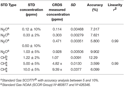
Table 2. Laboratory assays for N2O and CH4 calibrations using different gas standard concentrations injected directly into the CRDS.
FIGURE 3
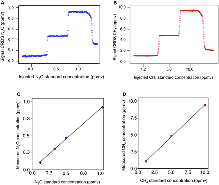
Figure 3. Raw CRDS data over the time series, obtained by injecting different standards with increasing concentrations for (A) nitrous oxide (B) methane and their respective calibration curves for (C) nitrous oxide and (D) methane.
Preliminary tests confirmed that the degassing membrane performed well with seawater at room temperature. Indeed, gas separation efficiency of the membrane was tested using equilibrated seawater with known N2O and CH4 gas levels (gas standards), and then measured using M-CRDS. This was carried out by filling GC vials (1 L) with seawater (previously equilibrated with the atmosphere) and hermetically sealed. Subsequently, seawater was replaced with 250 mL of standard gas to estimate the gas moles added into the vials. Then, dissolved gas concentration in the liquid phase was determined by Henry's law, taking into consideration temperature and salinity of the sample.
Figures 4A,B show dissolved gas concentrations obtained from equilibrating seawater and using gas standards injected into GC bottles measured by M-CRDS. Small differences were detected, with relative errors of 1.3 and 8.9% for N2O (Figure 4A) and CH4 (Figure 4B), respectively. The highest error was detected at high N2O concentrations, i.e., when a N2O standard of 1 ppm was injected, and the spectrometer measured 0.92 ppm. In addition, the M-CRDS method was subject to a specific response time (tr), which corresponds to the time required to reach a stable value indicated by PICARRO G-2308. This response time is illustrated in Figure 5. For example, a strong relationship (R2 = 0.995) was found between N2O concentration and response time of CRDS (tr = 14.93), using the model described in Equation (9).
FIGURE 4
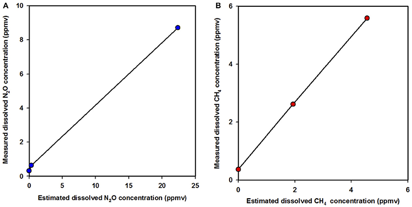
Figure 4. Linear regression between the estimated dissolved gases after reaching phases equilibrium and measured dissolved gas values using M-CRDS for (A) nitrous oxide and (B) methane. nitrous oxide (blue circle) and methane (red circle).
FIGURE 5
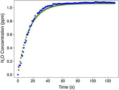
Figure 5. M-CRDS system response time to sudden N2O concentration changes in seawater (blue circles) as well as CN2O calculated from Equation (9) (green circles).
Table 3 compares dissolved gas concentrations measured using the M-CRDS and headspace-GC. The results revealed that both methods responded lineally to an increase in dissolved gas concentrations. Dissolved gas values measured directly by M-CRDS and headspace-GC (estimating the concentration of dissolved gases and phase equilibrium), were similar and relatively accurate, with an error <5%, except in the case of sample equilibrated with CH4 standard of 1937 ppmv (Table 3). Gas concentrations measured by headspace-GC methodology were slightly higher than M-CRDS; this difference may be due to the sample shaking time and variations in bottle size that could favor analyte transition from the aqueous to gaseous state (headspace). These results validated the methods used for obtaining high-resolution vertical measurements of GHGs in seawater.
TABLE 3
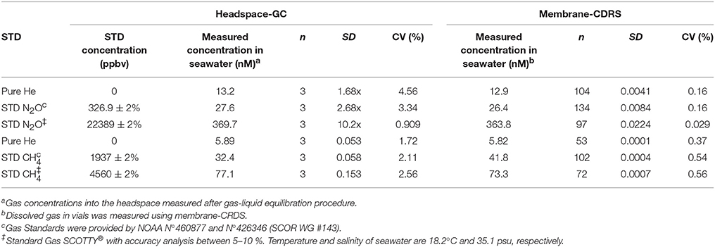
Table 3. Comparison of N2O and CH4 concentrations in seawater measured under laboratory conditions using headspace-GC and membrane-CRDS analysis.
Continuous Measurements of Physical and Biogeochemical Variables in the ESP
The ESP presented an extremely variable environment, with intense gradients in oceanographic and biogeochemical conditions. Chl-a, nutrient levels and euphotic layer thickness variability, is presented in Table 4. The centre of the subtropical gyre exhibited hyper-oligotrophy with levels of surface Chl-a as low as 0.03 mg m−3 and submicromolar nutrient levels, renowned for being the clearest waters of the global ocean (Raimbault et al., 2008; Morel et al., 2010). In contrast, the eutrophic zone associated with coastal upwelling presented Chl-a levels up to 4.84 mg m−3 and nutrient levels two orders of magnitude higher than those of the subtropical gyre. These conditions influence oxygen levels, as well as N2O and CH4 distribution which are sensitive to DO levels and organic matter availability.
TABLE 4
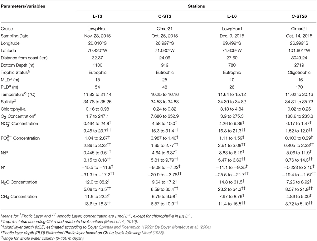
Table 4. Geographical, oceanographic and biogeochemical characteristics obtained from selected sampling stations.
Figures 6A–D show vertical profiles of temperature, salinity and DO, as well as water mass distribution at each station (Figures 6E–H). Station C-ST26 (Figures 6D,H) within the STPG was clearly influenced by the presence of Subtropical Water (STW), presenting more saline, warmer and oxygenated waters in comparison with coastal areas, i.e., station L-T3 (Figures 6A,E) and C-ST3 (Figures 6B,F). Near the coast, STW was confined to the narrow surface layer (0–30 m). Below the STW, Eastern South Pacific Intermediate Water (ESPIW, 30–60 m) and Equatorial Subsurface Water (ESSW; 100–300 m) were present, but the relative presence of each water mass and the degrees of mixing among water masses varied by latitude. ESSW is an important subsurface water mass in the ESP, as it carries O2 deficient waters poleward via the Peru-Chile Undercurrent (Huyer et al., 1991; Blanco et al., 2001). Remarkably, the northern station (L-T3 off Iquique at 20°S; Figures 6A,E) showed a subsurface minimum saline layer (MSL) associated with the presence of ESPIW at a depth between 20 and 50 m (σt = 25.7 ± 0.2). The ESPIW created a marked stratification of the water column, which seemed to favor a sharp DO gradient, as observed in station L-T3 and C-ST3 (Figures 6A,B). Subsequently, the presence of ESPIW diminished as it migrated southward (C-ST3 off Caldera at ~27°S and L-L6 off Coquimbo at ~29°S), and was replaced by Subantarctic water (SAAW) (Figures 6F–G).
FIGURE 6
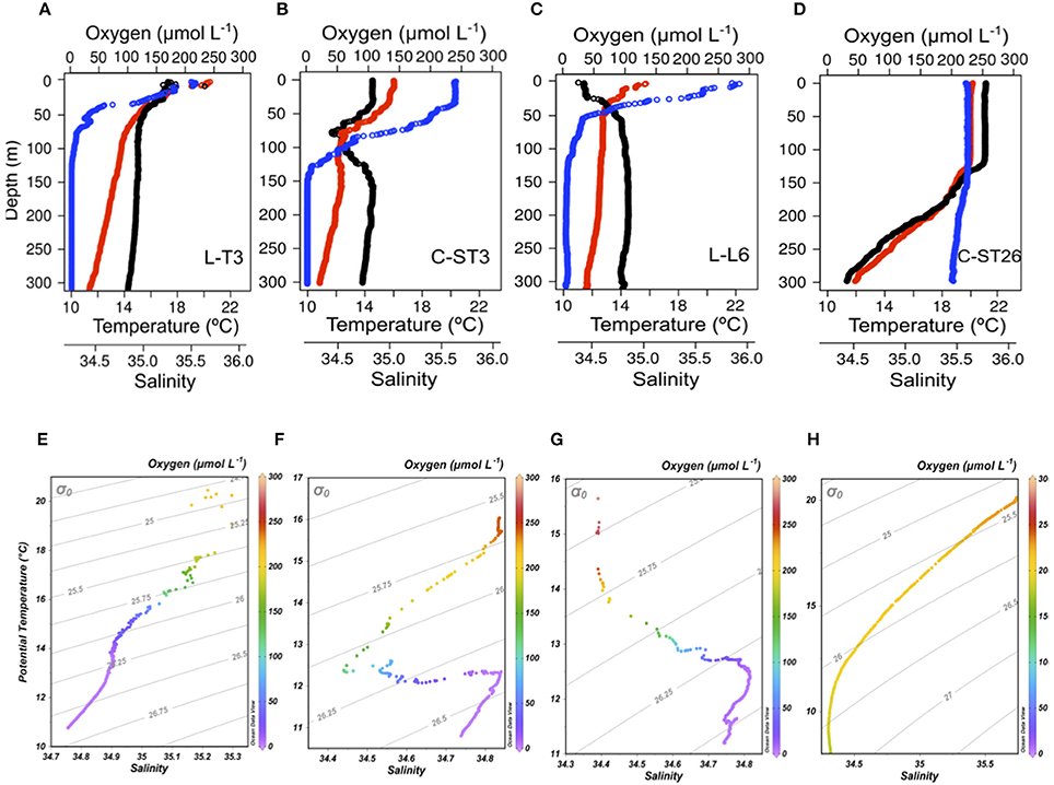
Figure 6. First row, high vertical resolution profiles of temperature (°C, red circle), salinity (black circle), and DO (μmol L−1, blue circle) obtained with CTD in selected stations ordered in columns at: (A) L-T3 the northernmost coastal area off Iquique (21°S), (B) C-ST3 coastal area off Caldera (27°S), (C) L-T6 the southernmost station in the coastal area and (D) C-ST26 at the subtropical gyre. Second row, T-S diagram for (E) LT3, (F) C-ST3, (G) L-T6, and (H) C-ST26 stations, showing the relative presence of water masses according to oceanographic locations; subtropical water (STW, σt = 25); Eastern South Pacific Intermediate Water (ESPIW, σt = 26); Equatorial Subsurface Water (ESSW, σt = 26.61) and SubAntarctic water (ASSW, σt = 25.83).
Vertical DO distribution at coastal stations was controlled by the presence of ESSW, demarcating OMZ, but also high primary production rates found in coastal areas. In general, in OMZs associated with upwelling areas, high organic production lead to enhanced O2 consumption through the decomposition of organic matter (Ulloa and Pantoja, 2009). Furthermore, DO distributions at eutrophic stations revealed the existence of sharp oxyclines; these gradients depended, at least partially, on the degradation of proteinaceous material during sinking through the OMZ, as quantified by sediment traps at 30 m (base of the oxygenated layer off northern Chile) (Pantoja et al., 2004). Organic matter sedimentation and the presence of a marked physical gradient, may cause the accumulation of organic matter (as observed in pycnoclines), as well as influence the locations of oxyclines (Farías et al., 2009). Indeed, at station L-T3 (~20°S), DO profiles showed a sharp oxycline, with the DO concentration decreasing from 247 μmol L−1 to 22.1 μmol L1 at the oxycline's lower limit (70 m depth) (Figure 6A). Below this depth, DO concentration reached <2.72 μmol L−1 (equivalent to 1.38% saturation) and remained relatively constant at OMZ's core, down to 300 m depth. This lower value may indicate a limitation of the applied CTDO methodology, as true values may have been even lower or zero (Canfield et al., 2010). DO at station C-ST3 presented a smoother distribution (Figure 6B) compared to station L-L6 (located in the southern part; Figure 6C), with DO values of 52.2 μmol L−1 at the oxyline base (100 m), compared to 24.9 μmol L−1 at 75 m (the oxycline base). Coincidentally, the latter station presented the highest Chl-a levels within the coastal zone sample stations, indicating that both pre-existing oxygenation levels and biological production regulated vertical DO distribution. Thus, DO distribution responds to a local balance between O2 production and its consumption, as well as physical processes. In contrast to results from stations within upwelling systems, a well-oxygenated water column was observed in a station located to the southern Subtropical Pacific Gyre (STPG) (C-ST26; Figure 6D).
Vertical Nutrient and GHG Distributions Measured by Continuous Methods
In addition to differences in DO, marked zonal differences in trophic levels have been also seen. This in turn affected nutrient availability and GHGs distribution in the ESP (Table 4). Figure 7 shows the vertical distribution of and obtained by continuous sampling with an autoanalyser coupled with the PPS. Coastal stations (L-T3, C-ST3, and L-T6, Figures 7A–C) presented , and levels that were two orders of magnitude higher, and had sharper gradients compared to station C-ST26 located in the STPG (Figure 7D), indicating the presence of coastal ESSW upwelling, as well as consumption by phyto and bacterioplankton. Within the mixed layer (photic layer) both and were as low as 0.46 and 0.98 μM, respectively, but never depleted. Underneath this layer, and gradually increased to maximum values of up to 9.18 and 2.20 μmol L−1 at the oxycline, respectively. The N2O maximum was observed at similar depths where nutricline (maximum concentration) was present (Figures 8A,B). Additionally, while slightly decreased toward the OMZ's core, gradually increased with depth, creating a Redfield deficit respect to . This depletion may be caused by a dissimilative reduction, denitrification, or even the anaerobic ammonium oxidation or anammox (Thamdrup et al., 2006; Farías et al., 2009) as was indicated by N* in coastal stations, which became increasingly negative with depth when DO decreased (Table 4).
FIGURE 7
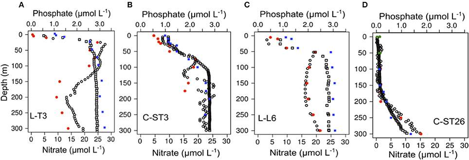
Figure 7. High vertical resolution profiles of nitrate (Black border circle) and phosphate (black border square) along with values of these nutrients obtained by discrete sampling (red dots and blue square, respectively) for stations (A): L-T3, (B): C-ST3, (C): L-T6, (D): C-ST26. Note that different sensitivities in concentration are displayed for nutrients at C-ST26 (green dot: nanomolar range in photic layer).
FIGURE 8
Figure 8. High vertical resolution profiles of nitrous oxide (gray circle) and methane (red circle) along with concentrations of those gases obtained by discrete sampling (blue dot for N2O; black dot for CH4) for (A) L-T3, (B) C-ST3, (C) L-T6, and (D) C-ST26 Stations.
By contrast, station C-ST26 was located within a region of anticyclonic wind stress curl with convergent Ekman transport at the gyre's core (negative Ekman pumping); there, a deep pycnocline, and low primary productivity were reported (Fiedler and Talley, 2006). Station C-ST26 presented a case of extreme oligotrophy and a well oxygenated water column (Figures 6D, 7D), with sub-micromolar levels of and in surface waters and severe nitrogen limitations, indicating that nutrients were predominantly supplied through regeneration (Bonnet et al., 2008; Claustre et al., 2008). In the STPG, N* presented positive values in the photic layer, and slightly negative values with increased depth (Table 4). Similar nutrient values and an excess of with respect to (according to Redfield ratio) have also been previously reported (Raimbault et al., 2008; Duhamel et al., 2017).
Figure 8 shows the vertical distributions of N2O and CH4 collected by continuous sampling with the M-CRDS coupled with the PPS. At the STPG (station C-ST26; Figure 8D), N2O distribution shows constant values within the photic layer and increased slightly with depth, up to 15.96 nM. With regards to coastal stations (Figures 8A–C), vertical gas distribution was predominantly dependent upon the oxycline and nutricline position (Figures 8A–C). N2O concentrations showed a marked peak at the oxycline with levels up to 31 nM, following a pronounced depletion of N2O below that peak, with undersaturated levels at the OMZ core (between 175 m and 300 m). A similar distribution of N2O has been observed for upwelling areas within the OMZ (Farías et al., 2009; Capelle et al., 2015; Ji et al., 2015), however, compared to previous observations (Farías et al., 2009), a deeper N2O maximum it is shown in this study. This variation is potentially due to shifts in the water column structure and dynamics associated with El Niño events, which produce a deepening of the thermocline, increased oxygenation and a reduced nutrient supply to the photic layer (Ulloa et al., 2001).
Despite CH4 oversaturation occurring throughout all studied stations, a distinct distribution in CH4 was observed between areas of coastal upwelling and the STPG. At the subtropical gyre (station C-ST26; Figure 8D), CH4 concentrations were relatively low and varied from 3.8 to 5.0 nmol L−1, with a slight peak at the subsurface layer (150–250 m depth). This peak was observed within the most stable layer, where particle accumulation occurred (Charpentier et al., 2007). Subsequently, CH4 levels decreased in intermediate waters. The values obtained in this study are slightly higher than those found previously in the STSP (Yoshikawa et al., 2014).
At the coastal stations, CH4 concentrations were considerably higher (7.72–23 nmol L−1) and showed a more complex distribution (Figures 8A–C). At the most northerly station (L-T3; Figure 8A), a clear CH4 peak occurred with values as high as ~23 nmol L−1 at 75 m depth within the photic zone and near the thermocline base (Figure 6A). High resolution analysis at station L-T3 showed several CH4 peaks and depletions, mostly superficially. At station C-ST3, CH4 concentrations peaked (up to 11 nmol L−1) at shallower depths near the oxycline's base (~75 m) (Figure 8B). In the aphotic layer, toward the OMZ's core, CH4 concentrations decreased slightly. Furthermore, lower values at station L-L6 (~150 m) compared to L-T3 (~100 m) were observed, with CH4 concentrations reaching 15.51 nmol L−1 (Figures 8A,C).
CH4 oversaturation has also been reported in surface waters of open ocean and upwelling systems. It is known as “the methane paradox” (Kiene, 1991). Several mechanisms might provoke CH4 oversaturation in oxygenated waters, where anaerobic methanogenesis should be inhibited (Sansone et al., 2001; Capelle et al., 2015; Chronopoulou et al., 2017). Methylotrophic micro-organisms play an important role in generating CH4 in oligotrophic waters (Damm et al., 2008; Karl et al., 2008; Repeta et al., 2016). In addition, anaerobic methanogens may be acting by micro-organisms attached to particles as was early reported by Lamontagne et al. (1973), and as it was observed in pycnoclines of our sampled stations (Figure 6).
Comparison of Gases and Nutrients Concentrations Obtained by Discrete an Continuous Sampling
Table 5 presents a comparison of analytical techniques used in this study for measuring N2O and CH4, where it can clearly be glimpsed the advantages and disadvantages comparatively. In addition, Figure 9 reveals a positive and significant correlation found for values obtained by continuous (membrane-CRDS) and discrete (headspace-GC) methods, with some deviations, particularly in N2O. These variations may be the result of instrument response time (tr) and PPS pumping speed, rather than analytical errors (Table 3; Figure 5). The errors were also observed predominantly at oxyclines and pycnoclines, layers with intense environmental variation, and where CRDS may be subject to rapid variations in gas concentrations, thus it is possible that water flows through the membrane faster than the instrument was able to react. The continuous method was subject to a delay due to the time required for the sample to reach the surface and pass through the degassing membrane. The time response (Equation 9; Figure 5) of the CDRS analyzer (PICARRO G-2308) was considered, as was performed by another similar study (Gonzalez-Valencia et al., 2014).
TABLE 5
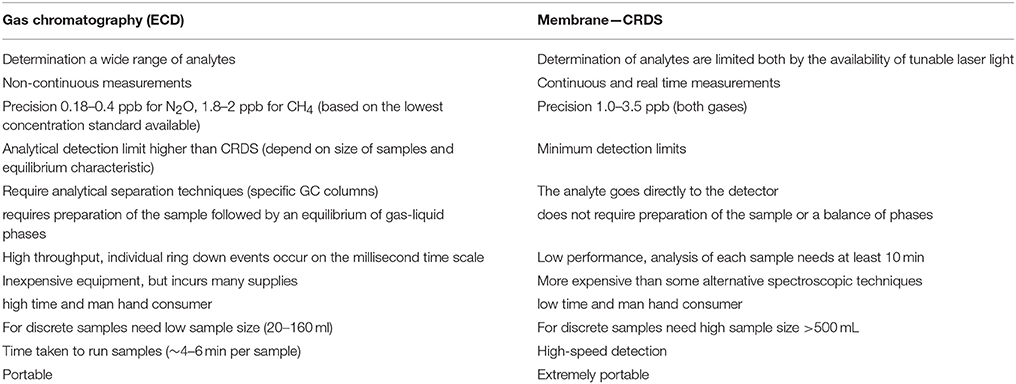
Table 5. Comparison of analytical techniques for measuring N2O and CH4.
FIGURE 9
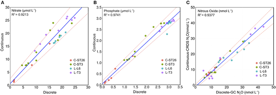
Figure 9. Regression of gas and nutrient concentrations at determined depths measured by GC and colorimetric methods in discrete samples, against alternative methods coupled with continuous sampling.
Both discrete and continuous methods also indicated a similar vertical pattern for and (Figure 7). Remarkably, at the STPG station, N2O and nutrient distributions throughout the water column remained fairly similar for both sampling techniques. But concentrations and also N2O collected during continuous sampling at coastal stations showed several peaks between 50 and 150 m within the OMZ's core. These results were not detected by discrete sampling. High-resolution vertical structures of and N2O were observed at coastal stations, particularly in C-ST3, within the OMZ. Within the OMZ, no vertical gradients were observed for physical variables, and therefore, and N2O values may be associated with coupling and reaction rates of different microbial processes, such as nitrification and denitrification (Codispoti and Christensen, 1985).
With regards to CH4, to date only few studies are available providing reference values for the subtropical ESP region (Florez-Leiva et al., 2013; Yoshikawa et al., 2014). Unfortunately, the small size of the data set from CH4 discrete samples meant that it was not possible to confirm these measurements, however the present values are lower than previous reports within the area and other similar areas (Sansone et al., 2001; Farías et al., 2009; Gonzalez-Valencia et al., 2014; Capelle et al., 2015), including the eastern Tropical North Pacific OMZ, with values as high as 105 nmol L−1 (Chronopoulou et al., 2017).
Conclusion and Recommendations
Traditional methodologies used for gas measurements are labor-intensive in terms of instrument operation and sample preparation, therefore affecting gas solubility. The methodology applied in this study involves the use of portable CRDS instrumentation, which is less complicated and faster than conventional laboratory-based techniques and allows the collection of real-time and continuous vertical gas distribution data in marine waters. Advantages of continuous measurements are that they provide high-resolution information from the water column, avoiding in situ errors, which mainly result from sample handling and external factors, such as temperature variations and atmospheric contamination. Continuous sampling can, therefore, effectively identify the biological processes influencing the OMZ characteristics and variability as a function of nutrient availability. This methodology avoids the sample preservation (which can produce erroneous data), and mercury chloride manipulation, an extremely toxic substance used for long-term gas and nutrient sample storage. Furthermore, coupling a degassing membrane (Permeselect-2500) with PICARRO G-2308 spectrometer notably reduces measurement times and delivers satisfactory results. In addition, new high-resolution vertical technologies (M-CRDS and LWCC) are developed and implemented giving real-time measurements. This furthers the general understanding of the biogeochemical processes involved in nutrient and gas cycling, and reveals new structures that cannot be observed by discrete sampling. This is especially valuable for areas with sharp gradients, such as oxyclines, where it is important to be able to identify the microbiological processes influencing variable distribution. High-resolution vertical profiles obtained for N2O, CH4 and nutrients in this study are similar to those estimated based on previous studies; nevertheless, in the case of N2O and even nutrients, this investigation revealed multiple vertical structures (peaks) that had not previously been observed. This methodology may uncover the presence of hotspots and “hot moments” at determined spatial and temporal scales, in a region affected by climate change, where an expansion of subtropical gyres and more intense coastal upwelling is predicted. Thus, these results offer alternative methods for measuring rates and pathways based on temporal and spatial conditions.
Author Contributions
All authors contributed extensively to the work presented in this paper. MT, GG and LF contributed to the development of the system and made all validation tests, JV and MT, GG carried out the on-board tests and the analysis of the data. LF contributed to the interpretation and writing of the paper. All authors discussed the results and commented on the manuscript at all stages.
Conflict of Interest Statement
The authors declare that the research was conducted in the absence of any commercial or financial relationships that could be construed as a potential conflict of interest.
Acknowledgments
Data was collected during the CIMAR 21 cruise (CONA CIMAR-21 Islas C21I 15-06) and the LowpHox I cruise (IMO ICM 120019 project). LF was supported by FONDECYT N°1161138 (LF). This research represents a contribution to the FONDAP (1511009) program. Time onboard was provided by the Chilean National Commission for Scientific and Technological Research (CONICYT) grant AUB 150006/12806. The authors express gratitude to Sam Wilson (University of Hawaii) and Fuminori Hashihama (Tokyo University of Marine Science and Technology) for their support in the namomolar determination of nutrients; Italo Masotti (CONA CIMAR-21 Islas C21I 15-12) and the IMO institute for providing Chl-a data for selected stations and Gadiel Alarcon who operated the PPS; and Caitlin Frame for her help during the LowpHox I cruise. We also thank Karla Martinez Cruz for her critical review and suggestions for improvements to our calculations.
Supplementary Material
The Supplementary Material for this article can be found online at: https://www.frontiersin.org/articles/10.3389/fmars.2018.00148/full#supplementary-material
Footnotes
References
Andrews, S. J., Hackenberg, S. C., and Carpenter, L. J. (2015). Technical Note: a fully automated purge and trap GC-MS system for quantification of volatile organic compound (VOC) fluxes between the ocean and atmosphere. Ocean Sci. 11, 313–321. doi: 10.5194/os-11-313-2015
Arevalo-Martinez, D. L., Beyer, M., Krumbholz, M., Piller, I., Kock, A., Steinhoff, T., et al. (2013). A new method for continuous measurements of oceanic and atmospheric N2O, CO and CO2: performance of off-axis integrated cavity output spectroscopy (OA-ICOS) coupled to non-dispersive infrared detection (NDIR). Ocean Sci. 9:1071. doi: 10.5194/os-9-1071-2013
Bange, H. W., Freing, A., Kock, A., and Löscher, C. R. (2010). Marine pathways to nitrous oxide. Nitrous Oxide Clim. Change 36–62. doi: 10.4324/9781849775113
Bates, T. S., Kelly, K. C., Johnson, J. E., and Gammon, R. H. (1996). A reevaluation of the open ocean source of methane to the atmosphere. J. Geophys. Res. Atmos. 101, 6953–6961. doi: 10.1029/95JD03348
Bell, R. J., Short, R. T., Van Amerom, F. H., and Byrne, R. H. (2007). Calibration of an in situ membrane inlet mass spectrometer for measurements of dissolved gases and volatile organics in seawater. Environ. Sci. Technol. 41, 8123–8128. doi: 10.1021/es070905d
Berden, G., and Engeln, R. (2009). Cavity Ring-Down Spectroscopy: Techniques and Applications. Chichester: John Wiley & Sons.
Blanco, J. L., Thomas, A. C., Carr, M. E., and Strub, P. T. (2001). Seasonal climatology of hydrographic conditions in the upwelling region off northern Chile. J. Geophys. Res. Oceans 106, 11451–11467. doi: 10.1029/2000JC000540
Bonnet, S., Guieu, C., Bruyant, F., Prášil, O., Van Wambeke, F., Raimbault, P., et al. (2008). Nutrient limitation of primary productivity in the Southeast Pacific (BIOSOPE cruise). Biogeosciences 5, 215–225. doi: 10.5194/bg-5-215-2008
Boutsiadou, X. (2012). Development of a System for “in situ” Determination of Chlorinated Hydrocarbons in Groundwater. Ph.D. dissertation, Université de Neuchâtel.
Brannon, E. Q., Moseman-Valtierra, S. M., Rella, C. W., Martin, R. M., Chen, X., and Tang, J. (2016). Evaluation of laser-based spectrometers for greenhouse gas flux measurements in coastal marshes. Limnol. Oceanogr. Methods 14, 466–476. doi: 10.1002/lom3.10105
Canfield, D. E., Stewart, F. J., Thamdrup, B., De Brabandere, L., Dalsgaard, T., Delong, E. F., et al. (2010). A cryptic sulfur cycle in oxygen-minimum–zone waters off the Chilean coast. Science 330, 1375–1378. doi: 10.1126/science.1196889
Capelle, D. W., Dacey, J. W., and Tortell, P. D. (2015). An automated, high through-put method for accurate and precise measurements of dissolved nitrous-oxide and methane concentrations in natural waters. Limnol. Oceanogr. Methods 13, 345–355. doi: 10.1002/lom3.10029
Charpentier, J., Farías, L., and Pizarro, O. (2010). Nitrous oxide fluxes in the central and eastern South Pacific. Global Biogeochem. Cycles 24, GB3011–GB3025. doi: 10.1029/2008GB003388
Charpentier, J., Farias, L., Yoshida, N., Boontanon, N., and Raimbault, P. (2007). Nitrous oxide distribution and its origin in the central and eastern South Pacific Subtropical Gyre. Biogeosciences Discussions, 4, 1673–1702.
Chronopoulou, P. M., Shelley, F., Pritchard, W. J., Maanoja, S. T., and Trimmer, M. (2017). Origin and fate of methane in the Eastern Tropical North Pacific oxygen minimum zone. ISME J. 11, 1386–1399. doi: 10.1038/ismej.2017.6
Claustre, H., Sciandra, A., and Vaulot, D. (2008). Introduction to the special section bio-optical and biogeochemical conditions in the South East Pacific in late 2004: the BIOSOPE program. Biogeosci. Discuss. 5, 605–640. doi: 10.5194/bgd-5-605-2008
Codispoti, L. A., and Christensen, J. P. (1985). Nitrification, denitrification and nitrous oxide cycling in the eastern tropical South Pacific Ocean. Mar. Chem. 16, 277–300. doi: 10.1016/0304-4203(85)90051-9
Crosson, E. R. (2008). A cavity ring-down analyzer for measuring atmospheric levels of methane, carbon dioxide, and water vapor. Appl. Phys. B Lasers Optics 92, 403–408. doi: 10.1007/s00340-008-3135-y
Damm, E., Kiene, R. P., Schwarz, J., Falck, E., and Dieckmann, G. (2008). Methane cycling in Arctic shelf water and its relationship with phytoplankton biomass and DMSP. Mar. Chem. 109, 45–59. doi: 10.1016/j.marchem.2007.12.003
De Boyer Montégut, C., Madec, G., Fischer, A. S., Lazar, A., and Iudicone, D. (2004). Mixed layer depth over the global ocean: an examination of profile data and a profile-based climatology. J. Geophys. Res. 109:C1200. doi: 10.1029/2004JC002378
De Brabandere, L., Canfield, D. E., Dalsgaard, T., Friederich, G. E., Revsbech, N. P., Ulloa, O., et al. (2014). Vertical partitioning of nitrogen-loss processes across the oxic-anoxic interface of an oceanic oxygen minimum zone. Environ. Microbiol. 16, 3041–3054. doi: 10.1111/1462-2920.12255
Denman, K. L., and Gargett, A. E. (1995). Biological-physical interactions in the upper ocean: the role of vertical and small scale transport processes. Ann. Rev. Fluid Mech. 27, 225–256. doi: 10.1146/annurev.fl.27.010195.001301
Duhamel, S., Björkman, K. M., Repeta, D. J., and Karl, D. M. (2017). Phosphorus dynamics in biogeochemically distinct regions of the southeast subtropical Pacific Ocean. Prog. Oceanogr. 151, 261–274. doi: 10.1016/j.pocean.2016.12.007
Farías, L., Castro-González, M., Cornejo, M., Charpentier, J., Faúndez, J., Boontanon, N., et al. (2009). Denitrification and nitrous oxide cycling within the upper oxycline of the eastern tropical South Pacific oxygen minimum zone. Limnol. Oceanogr. 54:132. doi: 10.4319/lo.2009.54.1.0132
Fiedler, P. C., and Talley, L. D. (2006). Hydrography of the eastern tropical Pacific: a review. Prog. Oceanogr. 69, 143–180. doi: 10.1016/j.pocean.2006.03.008
Florez-Leiva, L., Damm, E., and Farías, L. (2013). Methane production induced by dimethylsulfide in surface water of an upwelling ecosystem. Prog. Oceanogr. 112, 38–48. doi: 10.1016/j.pocean.2013.03.005
Fogler, H. S. (1992). Elements of Chemical Reaction Engineering. Upper Saddle River, NJ: Prentice-Hall.
Gonzalez-Valencia, R., Magana-Rodriguez, F., Gerardo-Nieto, O., Sepulveda-Jauregui, A., Martinez-Cruz, K., Walter Anthony, K., et al. (2014). In situ measurement of dissolved methane and carbon dioxide in freshwater ecosystems by off-axis integrated cavity output spectroscopy. Environ. Sci. Technol. 48, 11421–11428. doi: 10.1021/es500987j
Gordon, L. I., Jennings, J. C., Ross, A. A., and Krest, J. (1993). A suggested protocol for continuous flow automated analysis of seawater nutrients (phosphate, nitrate, nitrite and silicic acid) in the WOCE Hydrographic Program and the Joint Global Ocean Fluxes Study. Methods Manual WHPO 91-1, WOCE Hydrographic Program Office.
Grefe, I., and Kaiser, J. (2014). Equilibrator-based measurements of dissolved nitrous oxide in the surface ocean using an integrated cavity output laser absorption spectrometer. Ocean Sci. 10, 501–512. doi: 10.5194/os-10-501-2014
Griffith, T. D. (2015). Basic Principles and Calculations in Process Technology. Old Tappan, NJ: Prentice Hall.
Gruber, N., and Sarmiento, J. L. (1997). Global patterns of marine nitrogen fixation and denitrification. Global Biogeochem. Cycles 11, 235–266. doi: 10.1029/97GB00077
Huyer, A., Knoll, M., Paluszkiewicz, T., and Smith, R. L. (1991). The Peru Undercurrent: a study in variability. Deep Sea Res. A Oceanogr. Res. Papers 38, S247–S271. doi: 10.1016/S0198-0149(12)80012-4
Ji, Q., Babbin, A. R., Jayakumar, A., Oleynik, S., and Ward, B. B. (2015). Nitrous oxide production by nitrification and denitrification in the Eastern Tropical South Pacific oxygen minimum zone. Geophys. Res. Lett. 42, 755–764. doi: 10.1002/2015GL066853
Johnson, J. E. (1999). Evaluation of a seawater equilibrator for shipboard analysis of dissolved oceanic trace gases. Anal. Chim. Acta 395, 119–132. doi: 10.1016/S0003-2670(99)00361-X
Jones, A. W., and Schuberth, J. (1989). Computer-aided headspace gas chromatography applied to blood-alcohol analysis: importance of online process control. J. Forensic Sci. 34, 1116–1127. doi: 10.1520/JFS12748J
Karl, D. M., Beversdorf, L., Björkman, K. M., Church, M. J., Martinez, A., and Delong, E. F. (2008). Aerobic production of methane in the sea. Nature Geosci. 1, 473–478. doi: 10.1038/ngeo234
Kiene, R., and Service, S. (1991). Decomposition of dissolved DMSP and DMS in estuarine waters: Dependence on temperature and substrate concentration. Mar. Ecol. Progr. Seri. 76, 1–11. doi: 10.3354/meps076001
Kock, A., Arevalo-Martinez, D. L., Löscher, C., and Bange, H. W. (2016). Extreme N2O accumulation in the coastal oxygen minimum zone off Peru. Biogeosciences 13, 827–840. doi: 10.5194/bg-13-827-2016
Koroleff, F. (1983). “Determination of nutrients,” in Methods of Seawater Analysis, eds K. Grassoff, M. Ehrhardt, and K. Kremling (Weinheim: Verlag Chemie), 125–187.
Lamontagne, R. A., Swinnerton, J. W., Linnenbom, V. J., and Smith, W. D. (1973). Methane concentrations in various marine environments. J. Geophys. Res. 78, 5317–5324. doi: 10.1029/JC078i024p05317
Lepère, C., Vaulot, D., and Scanlan, D. J. (2009). Photosynthetic picoeukaryote community structure in the South East Pacific Ocean encompassing the most oligotrophic waters on Earth. Environ. Microbiol. 11, 3105–3117. doi: 10.1111/j.1462-2920.2009.02015.x
Li, Q. P., Hansell, D. A., and Zhang, J. Z. (2008). Underway monitoring of nanomolar nitrate plus nitrite and phosphate in oligotrophic seawater. Limnol. Oceanogr. Methods 6, 319–326. doi: 10.4319/lom.2008.6.319
Magen, C., Lapham, L. L., Pohlman, J. W., Marshall, K., Bosman, S., Casso, M., et al. (2014). A simple headspace equilibration method for measuring dissolved methane. Limnol. Oceanogr. Methods 12, 637–650. doi: 10.4319/lom.2014.12.637
Morel, A. (1988). Optical modeling of the upper ocean in relation to its biogenous matter content (case I waters). J. Geophys. Res. 93, 10749–10768. doi: 10.1029/JC093iC09p10749
Morel, A., Claustre, H., and Gentili, B. (2010). The most oligotrophic subtropical zones of the global ocean: similarities and differences in terms of chlorophyll and yellow substance. Biogeosciences 7, 3139–3151. doi: 10.5194/bg-7-3139-2010
Naqvi, S. W. A., Bange, H. W., Farías, L., Monteiro, P. M. S., Scranton, M. I., and Zhang, J. (2010). Marine hypoxia/anoxia as a source of CH4 and N2O. Biogeosciences 7, 2159–2190. doi: 10.5194/bg-7-2159-2010
O'Reilly, C., Santos, I. R., Cyronak, T., McMahon, A., and Maher, D. T. (2015). Nitrous oxide and methane dynamics in a coral reef lagoon driven by pore water exchange: Insights from automated high-frequency observations. Geophys. Res. Lett. 42, 2885–2892. doi: 10.1002/2015GL063126
Pantoja, S., Sepulveda, J., and Gonzalez, H. E. (2004). Decomposition of sinking proteinaceous material during fall in the oxygen minimum zone off northern Chile. Deep Sea Res. I Oceanogr. Res. Papers 51, 55–70. doi: 10.1016/j.dsr.2003.09.005
Patey, M. D., Rijkenberg, M. J., Statham, P. J., Stinchcombe, M. C., Achterberg, E. P., and Mowlem, M. (2008). Determination of nitrate and phosphate in seawater at nanomolar concentrations. TrAC Trends Anal. Chem. 27, 169–182. doi: 10.1016/j.trac.2007.12.006
Raimbault, P., Garcia, N., and Cerutti, F. (2008). Distribution of inorganic and organic nutrients in the South Pacific Ocean-evidence for long-term accumulation of organic matter in nitrogen-depleted waters. Biogeosciences 5, 281–298. doi: 10.5194/bg-5-281-2008
Ras, J., Claustre, H., and Uitz, J. (2008). Spatial variability of phytoplankton pigment distributions in the Subtropical South Pacific Ocean: comparison between in situ and predicted data. Biogeosciences 5, 353–369. doi: 10.5194/bg-5-353-2008
Reeburgh, W. S. (2007). Oceanic methane biogeochemistry. Chem. Rev. 107, 486–513. doi: 10.1021/cr050362v
Repeta, D. J., Ferrón, S., Sosa, O. A., Johnson, C. G., Repeta, L. D., Acker, M., et al. (2016). Marine methane paradox explained by bacterial degradation of dissolved organic matter. Nat. Geosci. 9, 884–887. doi: 10.1038/ngeo2837
Roberts, H. M., and Shiller, A. M. (2015). Determination of dissolved methane in natural waters using headspace analysis with cavity ring-down spectroscopy. Anal. Chim. Acta, 856, 68–73. doi: 10.1016/j.aca.2014.10.058
Sansone, F. J., Popp, B. N., Gasc, A., Graham, A. W., and Rust, T. M. (2001). Highly elevated methane in the eastern tropical North Pacific and associated isotopically enriched fluxes to the atmosphere. Geophys. Res. Lett. 28, 4567–4570. doi: 10.1029/2001GL013460
Snow, N. H., and Slack, G. C. (2002). Head-space analysis in modern gas chromatography. TrAC Trends Anal. Chem. 21, 608–617. doi: 10.1016/S0165-9936(02)00802-6
Sprintall, J., and Roemmich, D. (1999). Characterizing the structure of the surface layer in the Pacific Ocean. J. Geophys. Res. 104, 23297–23311. doi: 10.1029/1999JC900179
Stashenko, E. E., and Martínez, J. R. (2010). GC y GC-MS: Configuración del equipo versus aplicaciones. Sci. Chromatogr. 2, 25–51.
Thamdrup, B., Dalsgaard, T., Jensen, M. M., Ulloa, O., Farías, L., and Escribano, R. (2006). Anaerobic ammonium oxidation in the oxygen-deficient waters off northern Chile. Limnol. Oceanogr. 51, 2145–2156. doi: 10.4319/lo.2006.51.5.2145
Tilbrook, B. D., and Karl, D. M. (1995). Methane sources, distributions and sinks from California coastal waters to the oligotrophic North Pacific gyre. Mar. Chem. 49, 51–64. doi: 10.1016/0304-4203(94)00058-L
Ulloa, O., Escribano, R., Hormazabal, S., Quinones, R. A., González, R. R., and Ramos, M. (2001). Evolution and biological effects of the 1997–98 El Nino in the upwelling ecosystem off northern Chile. Geophys. Res. Lett. 28, 1591–1594. doi: 10.1029/2000GL011548
Ulloa, O., and Pantoja, S. (2009). The oxygen minimum zone of the eastern South Pacific. Deep Sea Res. II Top. Stud. Oceanogr. 56, 987–991. doi: 10.1016/j.dsr2.2008.12.004
Upstill-Goddard, R. C., Rees, A. P., and Owens, N. J. P. (1996). Simultaneous high-precision measurements of methane and nitrous oxide in water and seawater by single phase equilibration gas chromatography. Deep Sea Res. I Oceanogr. Res. Papers 43, 1669–1682. doi: 10.1016/S0967-0637(96)00074-X
Warner, N. R., Kresse, T. M., Hays, P. D., Down, A., Karr, J. D., Jackson, R. B., et al. (2013). Geochemical and isotopic variations in shallow groundwater in areas of the Fayetteville Shale development, north-central Arkansas. Appl. Geochem. 35, 207–220. doi: 10.1016/j.apgeochem.2013.04.013
Weiss, R. F., and Price, B. A. (1980). Nitrous oxide solubility in water and seawater. Mar. Chem. 8, 347–359. doi: 10.1016/0304-4203(80)90024-9
Wiesenburg, D. A., and Guinasso, N. L. Jr. (1979). Equilibrium solubilities of methane, carbon monoxide, and hydrogen in water and sea water. J. Chem. Eng. Data 24, 356–360. doi: 10.1021/je60083a006
Yoshikawa, C., Hayashi, E., Yamada, K., Yoshida, O., Toyoda, S., and Yoshida, N. (2014). Methane sources and sinks in the subtropical South Pacific along 17° S as traced by stable isotope ratios. Chem. Geol. 382, 24–31. doi: 10.1016/j.chemgeo.2014.05.024
Yver Kwok, C., Laurent, O., Guemri, A., Philippon, C., Wastine, B., Rella, C. W., et al. (2015). Comprehensive laboratory and field testing of cavity ring-down spectroscopy analyzers measuring H2O, CO2, CH4 and CO. Atmos. Meas. Tech. 8, 3867–3892. doi: 10.5194/amt-8-3867-2015
Zimmer, L. A., and Cutter, G. A. (2012). High resolution determination of nanomolar concentrations of dissolved reactive phosphate in ocean surface waters using long path liquid waveguide capillary cells (LWCC) and spectrometric detection. Limnol. Oceanogr. Methods 10, 568–580. doi: 10.4319/lom.2012.10.568
Keywords: continuous profiles, nitrous oxide, methane, nutrients, Eastern South Pacific
Citation: Troncoso M, Garcia G, Verdugo J and Farías L (2018) Toward High-Resolution Vertical Measurements of Dissolved Greenhouse Gases (Nitrous Oxide and Methane) and Nutrients in the Eastern South Pacific. Front. Mar. Sci. 5:148. doi: 10.3389/fmars.2018.00148
Received: 21 December 2017; Accepted: 11 April 2018;
Published: 26 April 2018.
Edited by:
Il-Nam Kim, Incheon National University, South KoreaReviewed by:
Manab Kumar Dutta, State Key Laboratory of Marine Environmental Science, Xiamen University, ChinaWei-dong Zhai, Shandong University, China
Copyright © 2018 Troncoso, Garcia, Verdugo and Farías. This is an open-access article distributed under the terms of the Creative Commons Attribution License (CC BY). The use, distribution or reproduction in other forums is permitted, provided the original author(s) and the copyright owner are credited and that the original publication in this journal is cited, in accordance with accepted academic practice. No use, distribution or reproduction is permitted which does not comply with these terms.
*Correspondence: Laura Farías, bGF1cmEuZmFyaWFzQHVkZWMuY2w=