The Spatial and Temporal Variability of Air-Sea CO2 Fluxes and the Effect of Net Coral Reef Calcification in the Indonesian Seas: A Numerical Sensitivity Study

A numerical model system was developed and applied to simulate air-sea fluxes of CO₂ and coral reef calcification in the Indonesian Seas and adjacent ocean basin for the period 1960–2014 on a fine resolution grid (ca. 11 km) in order to study their response to rising sea water temperatures and CO₂ concentrations in the atmosphere. Results were analyzed for different sub-regions on the Sunda Shelf (Gulf of Thailand, Malacca Strait, Java Sea) and show realistic and different levels, signs and pronounced temporal variability in air-sea CO₂ flux. The Gulf of Thailand changes from an atmospheric CO₂ sink during the boreal winter to a CO₂ source in summer due to higher water temperatures, while other sub-regions as well as the entire averaged Sunda Shelf act as a continuous source of CO₂ for the atmosphere. However, increasing atmospheric CO₂ concentrations weakened this source function during the simulation period. In 2007, the model simulations showed even a first flux inversion, in course of which the Java Sea took up CO₂. The simulated trends suggest that the entire Sunda Shelf will turn into a permanent sink for atmospheric CO₂ within the next 30–35 years if current trends remain constant. Considering the period between 2010 and 2014, coral reef calcification enhanced the average CO₂ emission of the Sunda Shelf by more than 10% from 15 to 17 Tg C yr⁻¹ due to lowering the pH and increasing the partial pressure of CO₂ in surface water. During the entire period of simulation, net reef calcification decreased although increasing seawater temperature mitigated effects of reduced CO₂ emission and the resulting decrease of the pH values on reef calcification. Our realistic simulation results already without consideration of any biological processes suggest that biological processes taking up and releasing CO₂ are currently well balanced in these tropical regions. However, the counteracting effects of climate change on the reef calcification, on other biological processes and the carbonate system need to be investigated in more detail. SST increased by about 0.6°C during the last 55 years, while SSS decreased by about 0.7 psu.

1. Introduction

The ocean-atmosphere CO₂ exchange process is quite well known (Wanninkhof, 1992, 2014, and others). It depends on the concentrations or partial pressures of CO₂ in the ocean surface water and the atmosphere and the gas transfer velocity. The oceanic CO₂ concentration is influenced by its solubility and, therefore, by the water temperature and salinity as well as the marine buffer system (alkalinity). It can change temporally and spatially due to physical and biogeochemical processes. The transfer velocity is related mainly to the wind speed above the ocean surface and the Schmidt number and temperature of the ocean surface water. In general, an atmospheric increase of CO₂ content leads to less CO₂ transfer from the ocean to the atmosphere or to more transfer into the other direction (or to a flux direction change). With this, the CO₂ concentration in the ocean increases resulting in the well known ocean acidification with all consequences to the marine ecosystem.

Air-sea fluxes of CO₂ between continental shelf and the atmosphere are still poorly quantified for the Indonesian Seas due to the poor data coverage, the complexity of the interacting processes and their response to increasing CO₂ concentrations in the atmosphere and the associated global warming (Cai et al., 2006; Chen and Borges, 2009; Doney et al., 2009; Takahashi et al., 2009; Borges, 2011; Wang et al., 2012; Bauer et al., 2013; Jones et al., 2014). Especially in the Indonesian Seas, independent model based estimated CO₂ fluxes along the coast disagree with air-sea fluxes of CO₂ derived from global ocean circulation models (Laruelle et al., 2014). The Sunda Shelf covers more than 20% of the global tropical shelf seas defined as regions less than 200 m deep between 23.4° southern and northern latitudes, i.e., 1.89 out of 9.21 10⁶ km², according to the 30″ × 30″ digital topography we used for this work (Farr et al., 2007). The Indonesian Seas are furthermore hot spots of coral diversity suffering from over-exploitation, global warming, and ocean acidification like all corals world wide (Cinner et al., 2016). The total area of corals in this region, 127,028 km², covers almost 30% of the global warm water coral reefs based on the global map from UNEP-WCMC et al. (2010) (423,582 km²). To our knowledge, Kartadikaria et al. (2015) are the first and so far only authors, who compiled detailed data on air-sea fluxes of CO₂ from the Indonesian Seas.

In contrast, the complexity of coral reef calcification, the interaction with reef pore water fluxes and changes in seawater chemistry have been studied intensively (Lough and Barnes, 1997; Langdon et al., 2000; Kleypas et al., 2006; Hoegh-Guldberg et al., 2007; Silverman et al., 2007; McGowan et al., 2016; Page et al., 2017, and many others). The application of numerical models incorporating observational findings and studying the impacts of rising CO₂ concentrations and sea water temperatures on the air-sea exchange of CO₂ and the reef calcification is missing so far on a horizontally fine resolved grid. Therefore, we developed a warm water coral reef calcification module for the regional biogeochemical ecosystem model ECOHAM and applied this on a fine-resolution 3D grid to the region of the entire Indonesian Seas to simulate the chemical carbonate system in this tropical marine environment.

The overarching goal is to get a principal idea about the spatial distribution and the long-term development of geochemical parameters, especially the exchange of CO₂ between ocean and atmosphere, under changing physical conditions (climate change and increasing atmospheric CO₂ content) and under the influence of carbonate precipitation with reliable rates from realistically distributed coral reefs. For this, a numerical model experiment has been performed to simulate the carbonate system in the tropical ocean (1) entirely without biological processes but under the influence of climate change and (2) additionally with aragonite precipitation only from coral reefs. The exclusion of biological processes in part (1) of our model experiment enables us to investigate the dependency of the carbonate system solely on the physical environment and on the changing atmospheric CO₂ content. The consideration of a net coral reef calcification rate in part (2) of our experiment helps to investigate the undisturbed effect of net coral reef calcification on that carbonate system and vice versa the effect of a changing physical environment on the calcification rate.

In the next section, we introduce our setting of the numerical models applied to simulate the hydrodynamics and to perform the experiment for the carbonate system without and with calcification from coral reefs. Then, hydrodynamic and the ecosystem model results will be verified. Thereafter, ecosystem model results will be presented as long-term time series for different sub-regions as well as for certain locations with different coral reef coverage. A discussion and a summary follow the data presentation.

2. Material and Methods: Applied Model System

The applied numerical model system consists in principle of a global general circulation model, which provides forcing data (sea surface height, temperature, salinity) at the open boundaries of a regional circulation model. Furthermore, a global hydrological model delivered river discharge data to the regional circulation model. This setup aimed at obtaining most realistic 2D and 3D time series for the physical conditions of the Indonesian Seas, especially for the water mass transports (velocities) and the 3D temperature and salinity distributions. Subsequently, an ecosystem model was applied on the same grid as the regional circulation model, of which the aforementioned physical parameters were used to simulate the chemical carbonate system.

Our regional model domain is presented in Figure 1. The horizontal grid resolution amounted to 6 min (approximately 11 km). In the vertical direction, 39 z layers with increasing thicknesses from 5 m at the surface to 550 m at greater depths resolved the bathymetry, which was limited to a maximum depth of 6,260 m.

FIGURE 1

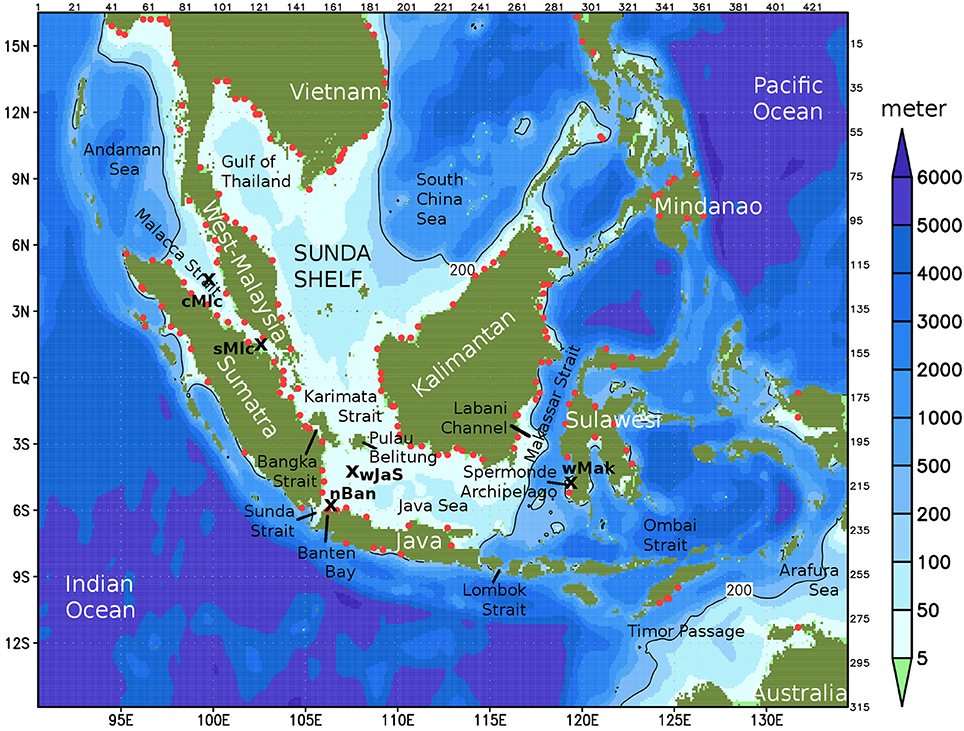
Figure 1. Regional hydrodynamical model domain with bathymetry. Red dots: river input points; X: locations to show single point time series of simulated carbonate system data. Isobath of 200 m is also drawn to depict the Sunda Shelf limit. Along the upper and right axes, model grid indices are shown.

2.1. Hydrodynamic Model

The global circulation model MPI-OM (Max Planck Institute Ocean Model, Marsland et al., 2003; Jungclaus et al., 2006), which is the oceanic part of the climate model system used for the IPCC world's climate simulations, was applied to the global ocean on the TP04 grid (Jungclaus et al., 2013), having a horizontal resolution of 24 min (approximately 44 km at lower latitudes) and 40 z layers of increasing thicknesses from top to bottom. Meteorological forcing data were taken from NCEP/NCAR (Kalnay et al., 1996). The reason for this first application step was to obtain high quality forcing data for the subsequently applied regional ocean circulation model HAMSOM (Hamburg Shelf Ocean Model, Backhaus, 1985; Pohlmann, 1996, 2006; Mayer et al., 2010), which used the vertical sections of temperature and salinity and the sea surface height as six hourly time series for its lateral open boundaries to the Indian Ocean, Pacific Ocean and South China Sea (Figure 1). HAMSOM is a prognostic baroclinic regional circulation model solving the momentum and tracer transport equations semi-implicitly on the Arakawa-C grid. Meteorological forcing data were taken from the same source (NCEP/NCAR) as for the global model.

Additionally, HAMSOM considers freshwater input through rivers into the ocean. These river discharge data were generated with the MPI-HM (Max Planck Institute Hydrology Model, Stacke and Hagemann, 2012), which is a global hydrological model solving the water balance on the land surface. The MPI-HM regularly takes part in model inter-comparison projects (Haddeland et al., 2011; Schewe et al., 2014). The input points for freshwater in the regional model domain are depicted by red dots in Figure 1.

For this investigation, long-term simulations were performed to analyse the development of properties over a period of more than 60 years. Therefore, daily averaged values were used to force the subsequently applied ecosystem model simulating the carbonate system.

2.2. Ecosystem Model

For the simulation of the carbonate system in the Indonesian Seas, ECOHAM (ecological model, Hamburg, Pätsch and Kühn, 2008; Kühn et al., 2010; Lorkowski et al., 2012; Große et al., 2016) has been applied on the same grid as the circulation model HAMSOM. ECOHAM is an NPZD-type ecosystem model simulating the cycles of nutrients (N, P, C, Si), of all species of dissolved inorganic carbonate (DIC), of O₂ and of total alkalinity (TA) and was originally developed to simulate biogeochemical processes including phyto- and zooplankton dynamics in the North Sea, which is located in the temperate climate zone. Parameters and limits in the process formulations of this model, in particular for biological processes, are adapted to that climate zone but not to the tropical zone. As a first step toward a fine resolution simulation of the carbonate system in the tropical ocean, we switched off the biological components in ECOHAM and used only the carbonate system part of the model. With this, it is possible to investigate the sensitivity of the carbonate system purely on physical environmental parameters plus the CO₂ concentration in the air. In a second step, we added a new module to simulate the CaCO₃ (only aragonite) precipitation due to calcifying corals to investigate also their influence on the carbonate system. This enables us to investigate the undisturbed effect of coral reef calcification on the carbonate system. Nutrients and their dynamics were not considered in these simulations (no biological components).

The principle way of simulating the carbonate system by ECOHAM is the following: transport and redistribution of concentrations of TA and DIC through the model grid by advection and diffusion with the velocities and turbulent diffusion coefficients provided by the regional circulation model HAMSOM. From the concentrations of DIC, the inorganic carbonate species dissolved CO₂, carbonic acid, bicarbonate and carbonate ions are calculated according to their solubility constants. Due to the CO₂ flux between ocean and atmosphere, DIC concentration can increase or decrease in the upper model layer. To provide the anthropogenic effect, a formula calculated the time dependent atmospheric CO₂ concentrations with best fit to observational data (Figure 2A), which have been kindly made available by Dlugokencky et al. (2017).

FIGURE 2

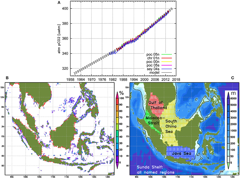
Figure 2. (A) Atmospheric CO₂ content in our simulations (black curve). Colored curves show measured data between 5 °N und 5 °S in the Pacific Ocean (poc) and the Indian Ocean (chr = Christmas Islands, sey = Seychelles). Measured data kindly made available by Dlugokencky et al. (2017). (B) Distribution of warm water corals in our domain in percent of the area of grid cells with coral reef presence. (C) Regions (colored shadings) referred to in this article for different spatial averages: Gulf of Thailand (red), Malacca Strait (green), Java Sea (blue). These three regions plus the southern South China Sea (yellow) make up our inner Sunda Shelf area.

As initial state and for the lateral open boundaries, different data sets of observed TA and DIC concentrations were taken from the CDIAC database Carbon Dioxide Information Analysis Center, RRID:SCR_006999, (Tilbrook et al., 2001; Johnson et al., 2002; Feely et al., 2007; Hydes et al., 2012; Kamiya et al., 2012; Tilbrook and Wijffels, 2012). These data from different ship cruises are very sparse in space and time for our region of interest. They were spatially extra- and interpolated to obtain a 3D distribution of DIC and TA concentrations in the model domain, which is not synoptic. However, there is currently no other way of creating such a fine resolved distribution of these parameters for this large domain.

2.3. Module to Simulate Net Coral Reef Calcification

For the simulation of precipitation of CaCO₃ (aragonite) from coral reef calcification, we basically follow the equation for the rate of calcification (Burton and Walter, 1987) and assume that the saturation of aragonite is drastically increased in the calcifying fluid due to the metabolism of the corals according to McCulloch et al. (2012).

$\begin{array}{ll}G=k{({\Omega }_{\mathrm{\text{a}}}-1)}^n& (1)\end{array}$

$\begin{array}{ll}\mathrm{\text{with }}{\Omega }_{\mathrm{\text{a}}}=\left[{\mathrm{\text{Ca}}}^{2+}\right]*\left[{\mathrm{\text{CO}}}_3^{2-}\right]/k_{\mathrm{\text{a}}}& (2)\end{array}$

G is the calcification rate (μmol m⁻² h⁻¹), Ω_a the saturation state of aragonite, k the rate constant (μmol m⁻² h⁻¹), n the order of reaction (Burton and Walter, 1987) and k_a the solubility constant for aragonite. k and n are functions of water temperature according to McCulloch et al. (2012), k_a is a function of temperature, salinity and pressure (Mucci, 1983; Millero, 1995).

Calcification is supposed to produce additional CO₂ in the ocean water:

$\begin{array}{ll}{\text{Ca}}^{2+}+2{\text{HCO}}_3^{-}\to {\text{CaCO}}_3+{\text{CO}}_2+{\text{H}}_2\text{O}.& (3)\end{array}$

Biomineralization is still a poorly understood process. Organic matter influences crystal growth and the morphology of carbonate skeleton, but calcification effects alkalinity and DIC as described in Equation. 3 according to our current understanding, as pointed out by Tambutté et al. (2011); McCulloch et al. (2012); Hohn and Merico (2015) and many more.

When applying Equations 1 and 2, we assumed that this corresponds to an average net coral reef calcification valid for the entire mix of different calcifying and decomposing reef organisms and for all coral reefs, as there are no data about the global distribution of dominant species with individual rates.

Furthermore, we assume a coral stimulated alteration of seawater properties within the calcifying fluid in the calicoblast, where corals calcify. The salinity dependent Calcium ion concentration ([Ca²⁺]) is increased by 0.5 mmol kg⁻¹, while the carbonate concentration ([${\text{CO}}_3^{2-}$]) is increased by a factor of 2 (McCulloch et al., 2012). With this, Equation 2 and subsequently Equation 1 are solved with the properties of the calcifying fluid. The calculated amounts of carbonate ions, which are taken out of the water due to the “carbonate precipitation,” are then deducted correspondingly from the DIC and TA pools.

Coral growth reduction and/or mortality during extreme events as seen during the ENSO periods in 1997/8 and 2015/16 are not considered in our simulations. Accordingly, increasing temperatures enhance the calcification process during the ENSO events in 1997/1998, when thermal stress caused an abnormally high coral mortality in the Indian Ocean (Wilkinson et al., 1999). Simulated coral growth rates are thus considered with great care. Due the short duration of extreme events, their overall impact on reef calcification and air-sea fluxes of CO₂ are assumed to be negligible, even though large areas of mortified coral reefs do have an impact on the local marine system.

In our model simulations, all the above described calcification related processes take place only in grid cells with a certain reef coverage. Using the UNEP global map of warm water coral reefs (UNEP-WCMC et al., 2010), which gives the presence of coral reefs on a grid with 30 × 30 s mesh size, a distribution of corals in our domain with 6 × 6 min resolution was calculated as coverage in percent of the horizontal area of each water column (see Figure 2B). The vertical location of the corals in the 3D model grid is the bottom layer but no deeper than 22 m (lower end of third layer).

2.4. Validation of Model Results

For the investigation of carbonate system related processes, it is essential to use a reliable distribution of temperature and salinity as well as transport of water masses. As examples to prove the high quality of our model results, the following sections will show the agreements of simulated and observation derived transports through key sections in our model domain to prove that the general simulated circulation is close to reality. Furthermore, a comparison between sea surface temperature and salinity data at certain locations will also prove realistic physical model results.

2.4.1. Simulated Averaged Transports Through Selected Sections

The averaged simulated transports through some important sections in the Indonesian Seas for the periods 2004–2006 and 1970–2006 are presented in Figure 3. To compare these data with estimations derived from observations, published values from van Aken et al. (2009), Sprintall et al. (2009), Gordon et al. (2012), and Feng et al. (2013) are listed in the figure as well.

FIGURE 3

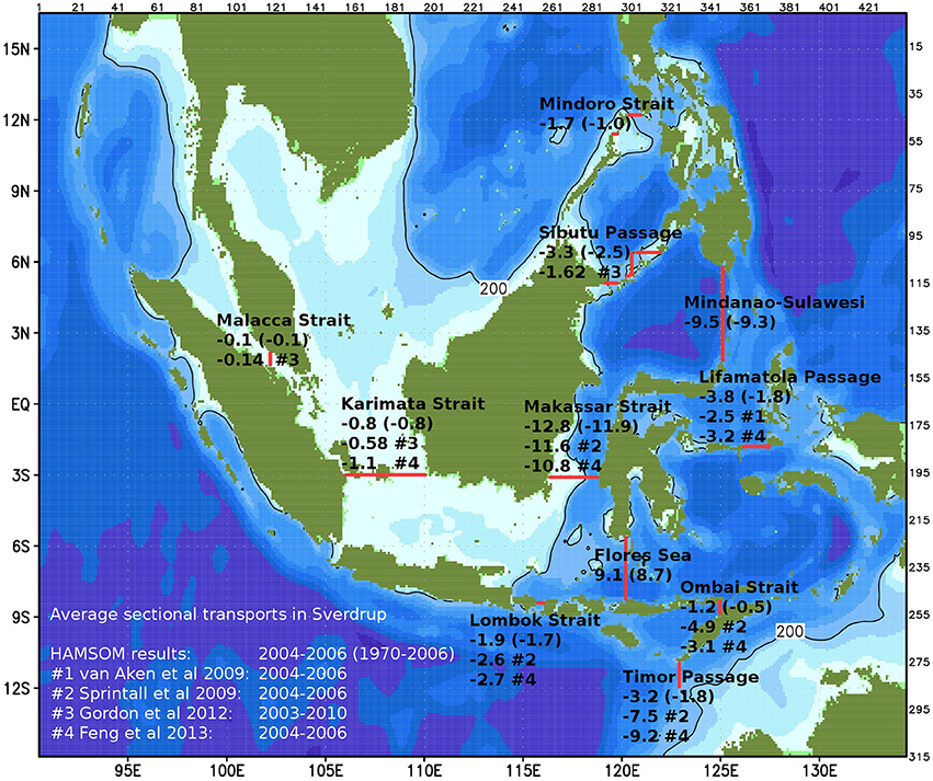
Figure 3. Simulated and literature referenced averaged transports through different sections for periods 2004–2006 and—in brackets—1970–2006 in Sverdrup (=10⁶ m³ s⁻¹), positive is north- or eastward, negative south- or westward. Upper lines display always the simulated and lower lines the cited values.

From the transport distributions, we can detect a principle agreement of the simulated with the expected circulation in the Indonesian Seas according to the cited literature. Remarkable differences occur for the Ombai Strait and Timor Passage transports, which is probably due to the fact that the southern part of the eastern open boundary cuts directly through the Arafura Sea between New Guinea and Australia. Obviously, in the model, a part of the water entering from the Pacific Ocean leaves through this open boundary instead of recirculating in the Arafura Sea and subsequently leaving the area through Ombai Strait and Timor Passage into the Indian Ocean.

The Lifamatola Strait value of −2.5 Sv (van Aken et al., 2009) represents only the depth range below 1250 m. The authors guess that there is rather a northward transport in upper regions of the passage leading to a total southward transport through this section of even less than 2.5 Sv. Our results of −3.8 Sv, however, correspond to the second cited value, −3.2 Sv, from Feng et al. (2013).

2.4.2. Comparison of Simulated SST and SSS With Satellite Data

The regional model HAMSOM agrees also well with real conditions concerning sea surface salinity (SSS) and temperature (SST). Both are shown in Figure 4 including a map for different locations.

FIGURE 4

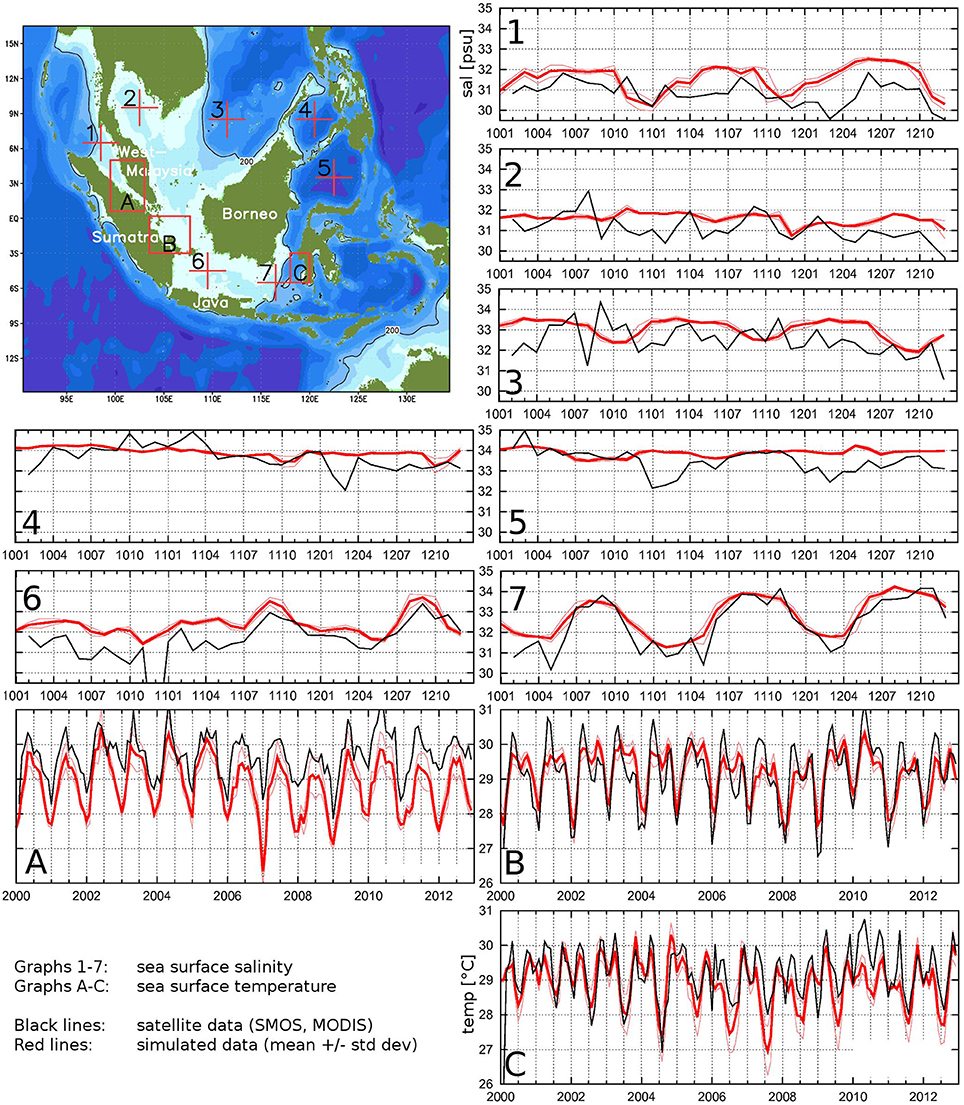
Figure 4. Simulated and satellite derived sea surface salinity (SSS) and temperature (SST) at different positions. Satellite SSS is from SMOS for 2010–2012, satellite SST from MODIS Aqua and Terra for 2000–2012.

For SST comparison, three regions A, B, C have been selected (see map in Figure 4): (A) a part of the Malacca Strait; (B) the Spermonde Archipelago near Makassar, Sulawesi; (C) an area east of middle-southern Sumatra coast including the Bangka Strait and the Siak river mouth, all for reasons of own field work performed during German-Indonesian cooperation projects. MODIS (Moderate-resolution Imaging Spectroradiometer) data from both EOS-Aqua and EOS-Terra satellites have been averaged temporally and horizontally over the corresponding depicted regions to obtain regional time series with monthly values. MODIS data have an accuracy of 0.4°C and represent surface squares of 4.6 km × 4.6 km. Simulated SST time series were created by averaging the upper layer temperature for the same regions and then temporally from daily to monthly data. When comparing the time series, we have to keep in mind that MODIS data are “skin temperatures” (Brown and Minnett, 1999). They are influenced by diurnal solar surface heating and by slight cooling due to evaporation (Minnett, 2003) with a heating effect much stronger than the cooling effect. An average of day and night remote sensing data leads therefore to slightly higher temperature data than the surface water would show. In contrast, the model results are “bulk temperatures” for the model's surface layer with a thickness of about 5 m plus the model's water level.

The comparison displayed in Figure 4 clearly shows that the seasonality as well as the level are in very good agreement, the seasonal peak values are over- or underestimated by no more than 1 K. It has been explained in the previous paragraph that the resulting MODIS averages are slightly higher than subsurface temperature. Therefore, model data are expected to be lower than these remote sensing data.

For SSS comparison, SMOS (soil moisture and ocean salinity sensor) derived data represent—with an accuracy of 0.4 psu—the upper ≈ 1 cm of the ocean surface (Boutin et al., 2014). They are available for horizontal areas of 1° × 1°, averaged from 3 days maps to monthly means. The simulated SSS data are again the values of the upper model layer (thickness: 5 m plus water level). The data were taken at the positions indicated in the map of Figure 4 and averaged to monthly values. The comparing time series are presented in panels 1–7 of Figure 4. Also here, a very good agreement of simulated and observed data is obvious for both the level and the seasonal variation if there is any. Differences are usually not more than 1 psu. It is impressive to see the seasonal variation at location 7, eastern Java Sea: During the first and last quarters of a year, the location is effected by relatively fresher water masses coming from the South China Sea, whereas during boreal summer season, this region is effected by the saltier Makassar Current coming from the North Pacific Ocean (Mayer and Damm, 2012).

A slight overestimation of SSS from the model is expected because of the thickness of the upper layer. Precipitation has a much larger impact on the remote sensing data than on the model data. Since the model does not resolve any vertical profile within the upper 5 m of the ocean, fresh water input from precipitation is immediately mixed into the upper 5 m layer, while the satellite sensor detects the fresher water within the upper ≈1 cm of the ocean. Because our locations are in the tropical zone with high rain fall rates, we expect the remote sensing data to be rather lower than the model data, which can indeed be seen in the comparing time series of Figure 4.

2.4.3. Comparison of Simulated and Observed Carbonate System Data and Calcification Rates

During a research cruise (MTK-2012, October 2012) with the vessel MatahariKu, the surface water pH and partial pressure of CO₂ in the water (pCO₂) was continuously measured by an underway pCO₂ system (SUNDANS) and a ferry box in the Bantan Bay (5.966°S, 106.134°E), a near-shore site about 70 km west of Jakarta. Wit et al. (2015) describe the method in detail, and Figure 5 presents the data. Based on the pH and pCO₂ values, the CO2sys program was used to calculate DIC and TA. These four parameters were compared with simulated data. The simulated data present daily means for each of the upper three layers at the time of the cruise for the grid point at the location of the measurements in the Banten Bay.

FIGURE 5

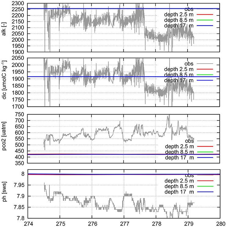
Figure 5. Simulated and measured TA (alk), DIC, partial CO₂ pressure (pco2), and pH in the surface water at Banten Bay, just north of western tip of Java. For the measured data, TA and DIC were calculated from the other two parameters. Labels along the x axis are Julian days of 2012 (274: 30 Sep).

This comparison shows that the model simulation overestimates TA by about 100 μmol kg⁻¹ and pH value by ca. 0.15 and underestimates pCO₂. Considering that Banten Bay is a near-shore and polluted area, the deviation might reflect the fact that the model TA is rather an open ocean value and not effected by near-shore ecosystems, since their benthic and pelagic biochemical activities are not considered in the simulations—e.g., Borges et al. (2005) show that the carbonate system in the coastal ocean exhibits different behavior compared to the open ocean (for example different air-sea CO₂ flux). Another possible reason for the differences is the quality of input data for the model, which is the best we could achieve within our study: TA is an averaged conservative tracer, interpolated from the CDIAC database and prescribed at the open model boundaries and transported by the currents into the model domain. Thus, it might not capture the specific situation in the Banten Bay.

A comparison of simulated carbonate system parameters (values and trends) with published estimations will be presented in the next section “Results”, also the good agreement of simulated calcification rates with published estimations from observations.

3. Results

Figure 6 presents the horizontal distribution of CO₂ flux between ocean and atmosphere in two different seasons (19 January and 13 July 2014). The overall distribution of uptake and outgassing is in good agreement with Kartadikaria et al. (2015), who analyzed a collection of observational data from the last few decades. Also, our simulated increase in pCO₂ of 76–120 μatm century⁻¹ is within their range of 60–380 μatm century⁻¹. In contrast to the Gulf of Thailand, parts of the Malacca Strait and the Karimata Strait, where the air-sea fluxes of CO₂ reverse on a seasonal cycle, the entire Sunda Shelf acts as a continuous source of CO₂ to the atmosphere. Consideration of coral reef calcification in the model (right panels) hardly affects the general pattern but causes small scale local differences in reef dominated regions. In these areas (e.g., northwest of Bangka Strait, in the Karimata Strait next to Pulau Belitung, and in the Spermonde Archipelago), calcification can even change the sign of the air-sea fluxes and convert CO₂ sinks into CO₂ sources for the atmosphere.

FIGURE 6

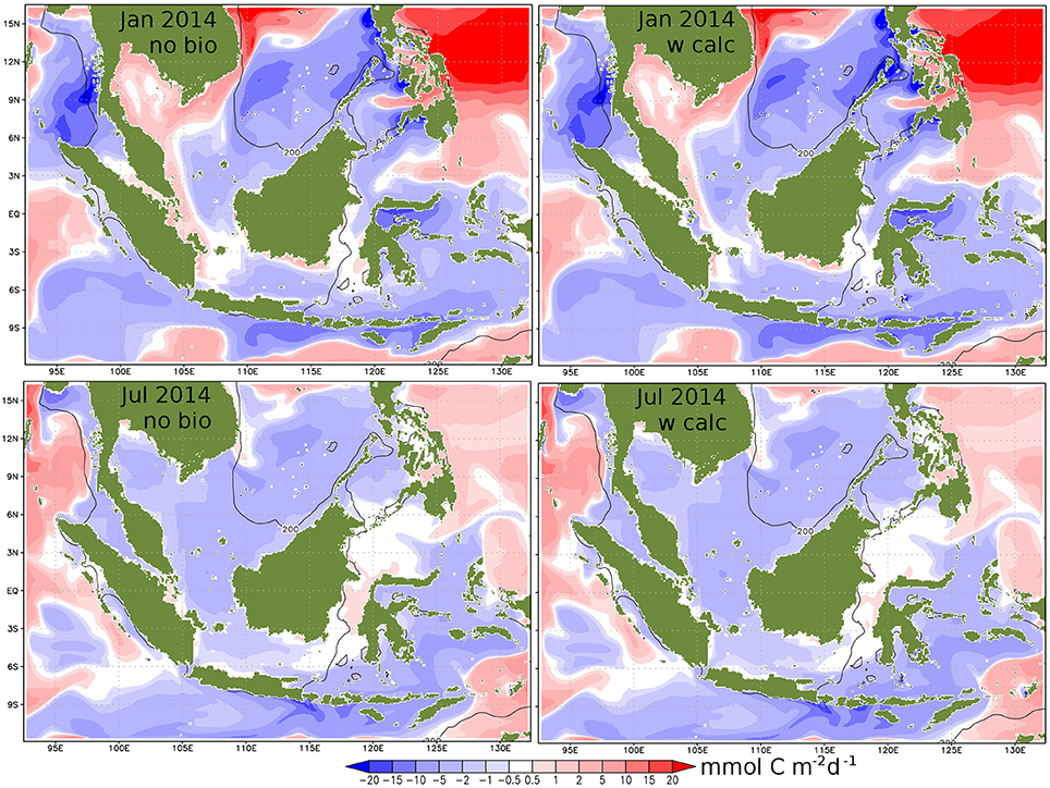
Figure 6. CO₂ flux between ocean and atmosphere (blue: oce⇒atm, red: atm⇒oce) for a day in January 2014 (upper) and in July 2014 (lower). Left display simulation results without biology, right with calcification. Maxima are around 25 mmol C m⁻² d⁻¹ in each direction.

To obtain spatial averages for the different sub-domains, 3D variables (TA, DIC, pCO₂, and pH) were volume weighted averaged, 2D variables (atm-oce CO₂ flux, SSS, and SST) were area weighted averaged, and directly reef dependent variables (Ω_a and calcification rate) were area weighted averaged over the corresponding coral reef areas according to the map in Figure 2B.

3.1. Carbonate System in Different Regions

The following carbonate system relevant parameters are presented in this section for the period 1960–2014 as spatial averages for different sub-domains: TA, DIC, pCO₂, air-sea CO₂ flux, pH value in seawater scale, Ω_a in seawater and in the calcifying fluid, aragonite calcification rate, SSS and SST. Figure 7 shows time series of yearly running means of the simulation results with corals for the inner Sunda Shelf, Gulf of Thailand, Malacca Strait and Java Sea, while Figure 8 displays time series of monthly values from both simulations without and with corals for the Java Sea (as an example) to display the role of coral reef calcification and the seasonality. In Table 2, average values for the last 5 years of simulation with coral reef calcification and trends in the time series from the last 50 years of simulation are given for all parameters and all sub-domains.

FIGURE 7

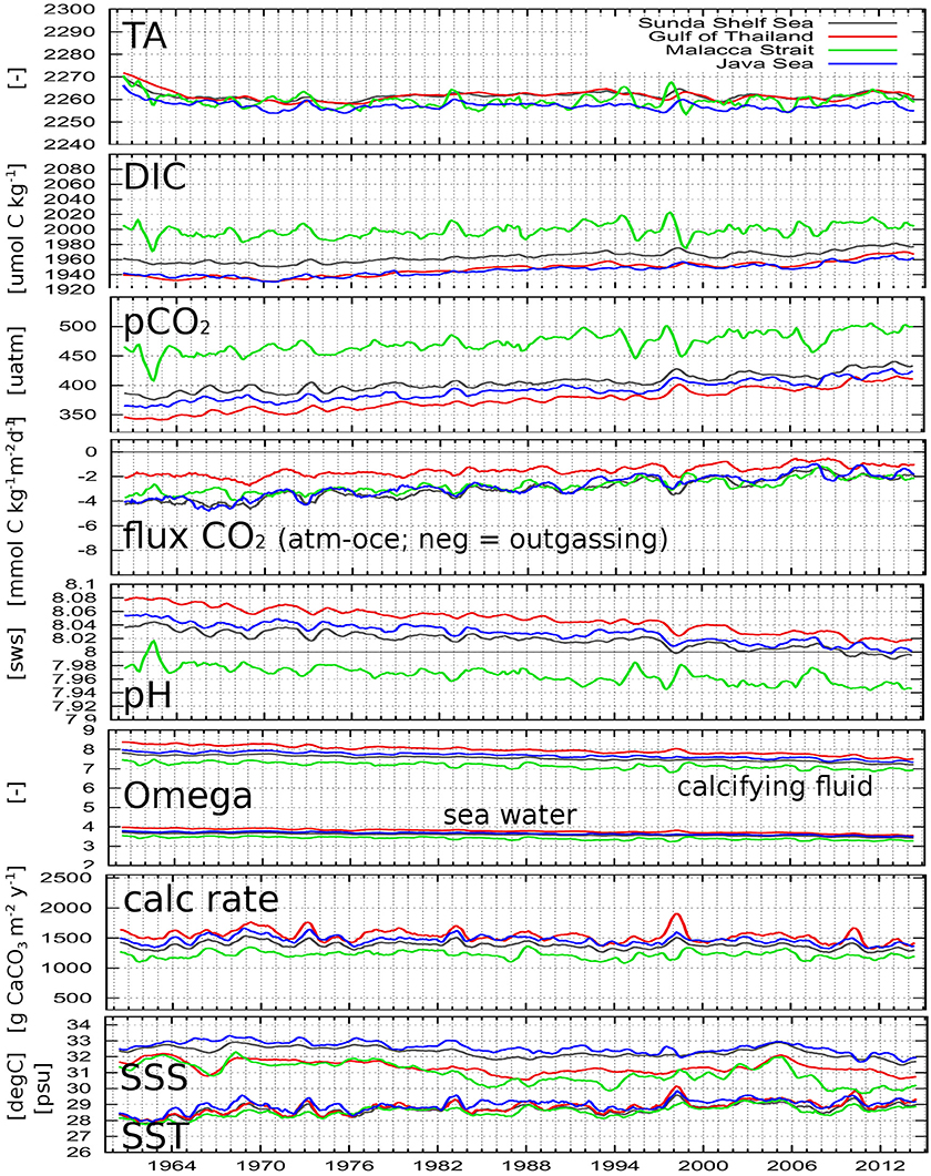
Figure 7. Simulated parameters as spatially averaged yearly running means for the entire Sunda Shelf Sea (gray), Gulf of Thailand (red), Malacca Strait (green), and the Java Sea (blue). pH is in seawater scale; “Omega” is the saturation state of aragonite; “calc rate” means aragonite calcification rate. Locations of regions are shown in Figure 2C.

FIGURE 8

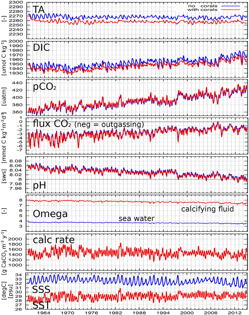
Figure 8. Simulated parameters as spatially averaged monthly means for the Java Sea without biological processes (blue) and with calcification (red). pH is in seawater scale; “Omega” is the saturation state of aragonite; “calc rate” means aragonite calcification rate. SSS and SST are for both simulations.

Looking at the long-term time series of the parameters in Figure 7, we see increasing values for DIC, pCO₂, and SST, and decreasing values of pH and Ω_a both in seawater and in the calcifying fluid, while the calcification rates and the CO₂ emissions slightly decrease.

The simulated range of pCO₂ increase of 76–120 μatm per century, corresponds well with values listed by Takahashi et al. (2009, Table 2) for different tropical regions in the Pacific and Indian Oceans, even though their values are open ocean surface values.

The simulated CO₂ flux to the atmosphere in the Sunda Shelf is in good agreement with estimations of Bauer et al. (2013). Our contemporary sea to air flux comes to ~8.4 g C m⁻² y⁻¹ on the average and about 0.017 Pg C y⁻¹ in total for the inner Sunda Shelf area (Table 2). This is ~21% of the global low latitude continental shelves' contribution as published by Bauer et al. (2013, 0.08 Pg C y⁻¹). Our inner Sunda Shelf covers about 23% of the global low latitude (<30°) continental shelf area (1.89 10⁶ km² out of 7.91 10⁶ km² according to Bauer et al. (2013). Laruelle et al. (2014) estimate a sea to air flux of 0.023 Pg C y⁻¹ for their region “South East Asia” representing an area of 2.3 10⁶ km², which is similar to our results. Cai et al. (2006) mention a slightly higher outgassing rate of 12 ± 5 g C m⁻² y⁻¹ for low latitude western and eastern boundary current shelves. Assuming that their estimations are based on older data and that there is a trend in the flux toward decreasing CO₂ emissions, our model results match their findings. Chen and Borges (2009) report in their Table 3 a much lower CO₂ outgassing rate of 1.2 g C m⁻² y⁻¹ for tropical continental shelves in the eastern Indian and western Pacific Oceans.

From the SST time series, we can observe temperature peaks in nearly all sub-domains for the year following a strong El Niño event (first half of 1973, 1983, 1998, 2010), the effect of which can be clearly detected in the calcification rate showing peaks at the same times, most obvious for the Gulf of Thailand, where the pH value is highest. The SSS time series do not show any ENSO response–except for the Java Sea, where we get a salinity peak during strong El Niño phases reflecting reduced precipitation rates.

To get an idea about the seasonality and the effect of calcification on the above mentioned parameters, Figure 8 presents the same parameters as monthly averages only for the Java Sea but as result from the simulation without biology and with calcification. There are clearly two different seasonal signals visible in the time series, which are introduced by the altering physical environment: Due to the Java Sea's geographical location close to the equator, the sun passes the region's zenith twice a year, producing two SST peaks per year (usually in Apr and Nov), with consequences on the solubility of CO₂ in the seawater and subsequently on pCO₂ and other parameters. Additionally, the predominant water flow direction alters seasonally: during boreal summer monsoon season, the westward flow transports rather saltier water from the Makassar Current, the extension of the Pacific North Equatorial and the Mindanao Currents, into the Java Sea, while fresher water from the South China Sea is transported eastward into the Java Sea during boreal winter monsoon season. This leads to one SSS peak usually in September and one minimum in January/February each year, which can be observed also in the time series for TA and DIC. The SST seasonality imprints its variability onto the time series of temperature dependent parameters such as solubility and the calcification process and, as a secondary effect, onto the others as well. Furthermore, in these Java Sea time series, the previously mentioned El Niño events are also visible (see peaks in SST, calcification rate and pCO₂, more negative CO₂ flux (more outgassing) and low pH values in 1973, 1983, 1997/1998).

Simulated calcification rates are shown in Table 2, Figures 7, 9 for different sub-regions and locations and in Figure 10 in different units. With 30–40 mmol CaCO₃ m⁻² d⁻¹, they are within but at the lower ends of globally observed ranges: Milliman and Droxler (1996, Table 1) publish a global mean coral reef calcification rate of 1,500 g CaCO₃ m⁻² y⁻¹ equal to 39 mmol CaCO₃ m⁻² d⁻¹. Silverman et al. (2007) mention observed rates between 30 ± 20 and 60 ± 20 mmol CaCO₃ m⁻² d⁻¹ in the northern Red Sea during boreal summer and winter, respectively, while DeCarlo et al. (2017) published a table of observed net ecosystem calcification rates (NEC) worldwide, depict the highest rate of 390 ± 90 mmol CaCO₃ m⁻² d⁻¹ in the South China Sea, and mention a worldwide average of reef flat NEC of 110–130 mmol CaCO₃ m⁻² d⁻¹.

TABLE 1

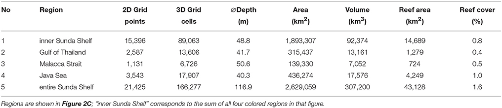
Table 1. Some geometric data about the sub-domains mentioned in the text.

It is obvious from Figures 7, 10 that the average net production of aragonite per unit area is highest in the Gulf of Thailand followed by the one in the Java Sea. However, due the smaller area, the total regional amount of calcified aragonite in the Gulf of Thailand is lower than in the Java Sea. The lowest net production occurred in the Malacca Strait falling below the one of the entire Sunda Shelf.

The carbonate precipitation did not effect the long-term trends described above but increased the pCO₂ and thus the CO₂ outgassing as expected. Nevertheless, in 2007, the increasing atmospheric CO₂ concentration exceeded for the first time the oceanic and turned the Java Sea into a CO₂ sink for a couple of months.

3.2. Carbonate System at Certain Points

For spatially non-averaged simulation results, seven different locations have been selected to present the differences of the simulation results “without-with” calcification, again as yearly running means, see Figure 9: two neighboring points (nBan) in the Banten Bay, just north of west Java Island, with 55 and 10% coral reef coverage, two almost neighboring points (wMak) in the Spermonde Archipelago, southern Makassar Strait, with 44 and 14%, and three points without any coral reefs: central western Java Sea (wJaS), central and southern Malacca Strait (cMlc, sMlc). All locations are marked in Figure 1.

FIGURE 9

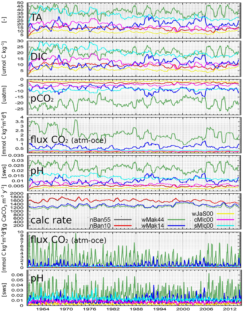
Figure 9. Differences of simulated parameters without-with reef calcification as yearly running means for certain grid points (see Figure 1). Colors are mapped to locations in the calc rate graph: nBan: north of Banten Bay, wMak: west of City of Makassar, wJaS: western Java Sea, cMlc/sMlc: central/southern Malacca Strait, numbers in location names mean % of reef coverage. pH is in seawater scale; “calc rate” is aragonite calcification rate (only simulation with corals). CO₂ flux and pH values are shown twice: the lower two panels are monthly values to visualize the seasonal variability.

FIGURE 10

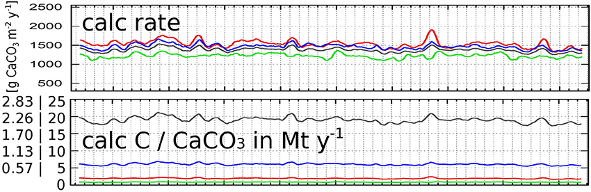
Figure 10. Simulated aragonite calcification rates as spatially averaged yearly running means for the entire Sunda Shelf Sea (gray), Gulf of Thailand (red), Malacca Strait (green), and the Java Sea (blue). Shown are the rates in g CaCO₃ m⁻² y⁻¹ (upper), and in Mt y⁻¹ of carbon and of aragonite.

The time series for both nBan locations nearly match each other, even though their reef coverage with 55 and 10% is quite different. Their calcification rates per m² are nearly the same because of similar water properties at both locations–due to the current system and the resulting dispersion. The calcified mass (not shown), however, is much larger at nBan55 due to the higher coral occurrence. In contrast to this, both wMak points (44 and 14%, green and blue curves in Figure 9), which are not direct neighbors, show slightly different but comparable calcification rates per m², but their unequal calcified masses, due to different coral occurrence, influence the water properties in their grid cells also quite differently. As expected, the changes in the wMak44 water are larger for all parameters, e.g., with higher pH decrease of around 0.025 at wMak44 vs. 0.01 at wMak14, higher pCO₂ increase of 15-25 μatm at wMak44 vs. 5–15 μatm at wMak14. This leads also to a stronger increased CO₂ release at wMak44 than at wMak14.

Naturally, dispersion of properties plays also an important role in marine environments. This is evident from the time series of the three locations without any coral coverage (wJaS00, cMlc00, sMlc00), where the visible differences between simulation results without and with calcification in Figure 9 were not locally generated but transported to these places.

To stronger illuminate the variability, the lower two panels of Figure 9 display monthly averages instead of yearly running means for two important parameters, the atmosphere-ocean CO₂ flux and the pH value. Seasonally and locally (e.g., at wMak44, green curves), the pH value can decrease by up to 0.06 units, and the CO₂ outgassing can increase by up to almost 10 mmol C m⁻² d⁻¹.

4. Discussion

In this section, we discuss our model results according to the most important processes we aimed to investigate in this first step of our model application: the air-sea flux of CO₂, the ocean acidification, and the coral reef calcification. They are connected to each other, because the first one has implications on the second and subsequently on the third one.

In the previous section, we have shown that our model results agree quite well with observational data already for the first part of simulation, which was without any biological processes. This might suggest that the basic biological processes in the tropical shelf sea—photosynthesis, respiration, calcification, dissolution—are overall well balanced. The consideration of realistic net coral reef calcification rates leads to a slight change of geochemical parameters in the seawater and in the exchange of CO₂ between ocean and atmosphere. Obviously, this has an overall moderate impact on the carbonate system in the tropical shelf sea, which might, however, alter with climate change effecting the several involved processes differently.

4.1. Air-Sea Fluxes of CO₂

For the entire Sunda Shelf, the air-sea CO₂ exchange are generally directed from ocean to atmosphere with a seasonal variation due to the seasonality of the atmospheric CO₂ concentration. In some areas like the Gulf of Thailand, emission of CO₂ occurs only seasonally, in other parts like the Java Sea, seasonal CO₂ uptake started in recent years. Obviously, there is a trend toward less outgassing or more uptake for all areas superimposed by the trend of growing atmospheric CO₂ content. Assuming constant trends in atmospheric CO₂ concentration, in SSS and SST development, according to Table 2, there will be no CO₂ emission in the Sunda Shelf domain any more after 30–35 years–with all consequences on the ocean acidification and the marine biology.

TABLE 2

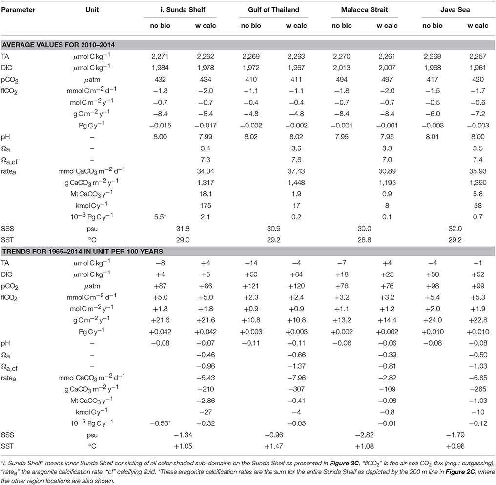
Table 2. Averages (2010–2014) and trends (1965–2014, 50 years, in units per century) in simulated time series without biology (“no bio”) and with calcification (“w calc”).

The effect of Equation 3 showing the production of CaCO₃ and additional CO₂ in the seawater is a shift of the curve of air-sea CO₂ flux toward more emission. For the Sunda Shelf water, this effect amounts to about 10% from 15 to 17 Tg C y⁻¹ because of the overall small coral reef coverage. For local areas, however, the effect can be as high as visible in Figure 9 by the green curve showing an increase of outgassing by up to 3.5 mmol C m⁻² d⁻¹ for a location with a 44% coral reef coverage.

4.2. Ocean Acidification

The simulated trend for the pH values (see Table 2: decrease of around 0.1 per century) is consistent with publications for other regions (e.g., Santana-Casiano et al., 2007, Canary Islands, around 0.1 units per century). This indicates that biological processes may not change the trend significantly. Most likely, they influence the pH level, correspondingly to what we found in our results without and with coral reef calcification. Following DeCarlo et al. (2017), the consideration of biological processes in coral reefs would increase the pH value and also the aragonite saturation state because of net CO₂ fixation from net ecosystem production (NEP). This would, in turn, enhance NEC. But NEC would reduce the pH value again. Also Silverman et al. (2007) found from their observations a dependency of NEC on nutrient concentrations, which corresponds to a dependency of NEC on NEP.

Therefore, the consideration of biological processes other than reef calcification by means of NEP would, on the one hand, lead to an increase of the pH level and a subsequent increase of calcification rates, which would then, on the other hand, lower the pH level again. The estimations of the net effect of NEP plus NEC, i.e., the balanced state at the end including the rates of NEP and NEC, was not possible within the current study. However, it would definitely be a further research project worth to be performed.

In other intensively studied shelf areas like the North Sea, biological processes such as CO₂ uptake during photosynthesis and its subsequent export into sub-surface water or directly into the underlying sediment strongly influence the air-sea fluxes of CO₂ (Lorkowski et al., 2012). In their studies, this function was declining during 1970-2006. Others like Metzl et al. (2010) found also declining carbon shelf pumping effected by increasing SST and decreasing pH values. Similar results were obtained by Lauderdale et al. (2016). These authors quantified the air-sea CO₂ flux drivers and find an oceanic CO₂ uptake due to biological activity, opposing all other drivers, for the tropical Indian, Pacific and Atlantic Oceans. However, their findings result from investigations in the open ocean and are not necessarily valid for a tropical shelf sea like the Sunda Shelf region.

4.3. Coral Calcification

Our estimated calcification rate for the entire Sunda Shelf amounts to 5.5 Tg C y⁻¹ (Table 2). Bauer et al. (2013) give a rate of 150 Tg C y⁻¹ for the global coastal inorganic carbon burial, Chen and Borges (2009) publish a rate of 180 Tg C y⁻¹ for the global particulate inorganic carbon burial including the fish catches on shelves. Therefore, according to our model results, the contribution of the coral reef calcification only on the Sunda Shelf is 3–4% of the global coastal carbon extraction. If we take this percentage for all warm water coral reefs and assume that the reef area on the entire Sunda Shelf amounts to 10% of the global coral area (see Introduction and Table 1: 43,128 out of 423,582 km²), the global contribution of warm water coral reef calcification to the permanent extraction of inorganic carbon from the water column would be 30–40%.

For the simulation of the calcification process in a coral reef, we applied an equation for the net calcification rate, which represents the gross calcification minus biological and chemical dissolution (NEC of the entire coral reef communities). However, dissolution of CaCO₃ is not necessarily a certain and constant proportion of the calcified aragonite mass as published for example by Silverman et al. (2007). Therefore, an improvement of the model results would be a consideration of dissolution rates to make this process depend on the aragonite saturation and the temperature in the seawater, possibly also on the nutrient concentration.

As obtained from the model results, the trend of SST is an increase by more than 1°C per 100 years, which has an enhancing effect on the calcification process (Cooper et al., 2012). The pH values are decreasing by 0.07–0.11 units per 100 years, which is lowering the calcification rate (Kleypas et al., 2006; Hoegh-Guldberg et al., 2007). Hence, these two trends have an opposing effect on the calcification process. However, according to our model results, the dominant component is the pH value reducing the availability of ${\text{CO}}_3^{2-}$ in the calcifying fluid when decreasing in the seawater. Additionally, the SSS time series show also a decreasing trend (1–2.8 psu per 100 years), due to increasing precipitation (rain), reducing the availability of Calcium necessary for calcification.

5. Summary and Conclusions

A numerical model system was applied to the tropical Indonesian Seas to simulate the CO₂ air-sea flux under the influence of increasing atmospheric CO₂ and under the additional influence of aragonite calcification from coral reefs for a period of almost 60 yeas. As a first step, simulations were performed without consideration of any biological processes. The long-term time series show realistic values and trends for relevant geochemical parameters of the physical and carbonate systems, supporting the findings of other authors regarding ocean acidification. The good agreement of these simulation results (no biological processes) with estimations from observational data suggests that biological processes taking up and releasing CO₂ are currently well balanced in these tropical regions. As a second step, we repeated the simulation but considered reef calcification, achieving realistic results for the calcification rates (around 1,400 g CaCO₃ m⁻² y⁻¹). The effect of this was an increase of CO₂ emissions. During the period from 2010 to 2014, calcification enhanced the average CO₂ emission of the Sunda Shelf by more than 10% from 15 to 17 Tg C yr⁻¹ due to lowering the pH and increasing the pCO₂ in surface water. The long-term simulation results for the total rate of reef calcification as well as a lowering of reef calcification rate.

The Sunda Shelf region used to be generally a source of CO₂ for the atmosphere. However, influenced by increasing sea surface temperatures, enhancing outgassing, and increasing atmospheric CO₂ concentrations, damping outgassing, the CO₂ emissions were reduced on the Sunda Shelf. In some parts, the CO₂ flux was even reversed to oceanic uptake. Overall, the entire Sunda Shelf is expected to turn into a permanent atmospheric CO₂ sink within the next 30–35 years, assuming that our estimated trends are constant. On the long-term, this definitely would have a severe impact on the marine biological environment.

One of our major findings from our simulations is that tropical marine environments are really not all the same. It is possible and necessary to distinguish different regimes even within the limited Sunda Shelf region. They show different influences from calcification, different behavior in the carbonate system with some regions acting as a CO₂ source and others as a CO₂ sink for the atmosphere, and—more important—different trends in the long-term time series. This points out that it is important but not sufficient to investigate the global impact of climate change, because consequences on the regional scale might significantly defer from the global overall results and be much more severe.

To obtain further realistic and reliable results, especially for climate projections, the simulation of net reef calcification should consider both aragonite production and dissolution rates, not only an overall net rate, as well as primary production and respiration processes, because the several components might change differently with climate change. Furthermore, a temperature dependent limitation of coral growth will be incorporated to enable a consideration of further relevant processes like coral bleaching. This, however, depends on the availability of a comprehensive data inventory for this region, which provides corresponding and consistent biogeochemical and nutrient data to initialize and force the numerical model.

Author Contributions

BM: Did most of research published. TR: Gave worthy research questions and expertise recommendations, took part in writing the manuscript. TP: Gave worthy research questions and expertise recommendations, did manuscript reviews, PI for the project.

Conflict of Interest Statement

The authors declare that the research was conducted in the absence of any commercial or financial relationships that could be construed as a potential conflict of interest.

The handling Editor declared a shared affiliation, though no other collaboration, with one of the authors (TR).

Acknowledgments

This project was funded by the German Ministry of Education and Research under the grant 03F0642D in the frame of the German-Indonesian cooperation SPICE III.

We would like to thank the Japan Meteorological Agency for hosting the website of World Meteorological Organization's (WMO) World Data Centre for Greenhouse Gases (WDCGG) and also the National Oceanic and Atmospheric Administration (NOAA) of the U.S.A. for providing the greenhouse gas data (measured atmospheric CO₂) via http://ds.data.jma.go.jp/gmd/wdcgg or ftp://aftp.cmdl.noaa.gov/data/greenhouse_gases/co2/flask. Their data were basis to derive our formula for the atmospheric CO₂ concentration in our model simulations.

Furthermore, we would like to thank the Carbon Dioxide Information Analysis Center (CDIAC), located at the U.S. Department of Energy's (DOE) Oak Ridge National Laboratory (ORNL), for providing global oceanic carbonate data (TA, DIC) via their website http://cdiac.ornl.gov.

We are also thankful to Francisca Wit (Leibniz Centre for Tropical Marine Research, Bremen, Germany) for offering their measured data collected during our joint research cruises in Oct 2012 and April 2013, which we used for comparison with model results.

References

Backhaus, J. O. (1985). A three-dimensional model for the simulation of shelf sea dynamics. Deutsche Hydrographische Zeitschrift 38, 165–187.

Google Scholar

Bauer, J. E., Cai, W.-J., Raymond, P. A., Bianchi, T. S., Hopkinson, C. S., and Regnier, P. A. G. (2013). The changing carbon cycle of the coastal ocean. Nature 504, 61–70. doi: 10.1038/nature12857

PubMed Abstract | CrossRef Full Text | Google Scholar

Borges, A. V. (2011). Present Day Carbon Dioxide Fluxes in the Coastal Ocean and Possible Feedbacks Under Global Change. Dordrecht: Springer.

Google Scholar

Borges, A. V., Delille, B., and Frankignoulle, M. (2005). Budgeting sinks and sources of CO₂ in the coastal ocean: diversity of ecosystems counts. Geophys. Res. Lett. 32:L14601. doi: 10.1029/2005GL023053

CrossRef Full Text | Google Scholar

Boutin, J., Martin, N., Reverdin, G., Morisset, S., Yin, X., Centurioni, L., et al. (2014). Sea surface salinity under rain cells: SMOS satellite and in situ drifters observations. J. Geophys. Res. Oceans 119, 5533–5545. doi: 10.1002/2014JC010070

CrossRef Full Text | Google Scholar

Brown, O. B., and Minnett, P. J. (1999). MODIS Infrared Sea Surface Temperature Algorithm Theoretical Basis Document, Version 2.0. Miami, FL: University of Miami.

Google Scholar

Burton, E. A., and Walter, L. M. (1987). Relative precipitation rates of aragonite and Mg calcite from seawater: temperature or carbonate ion control? Geology 15, 111–114. doi: 10.1130/0091-7613(1987)15<111:RPROAA>2.0.CO;2

CrossRef Full Text | Google Scholar

Cai, W.-J., Dai, M., and Wang, Y. (2006). Air-sea exchange of carbon dioxide in ocean margins: a province-based synthesis. Geophys. Res. Lett. 33:L12603. doi: 10.1029/2006GL026219

CrossRef Full Text | Google Scholar

Chen, C.-T. A., and Borges, A. V. (2009). Reconciling opposing views on carbon cycling in the coastal ocean: Continental shelves as sinks and near-shore ecosystems as sources of atmospheric CO₂. Deep Sea Res. II Top. Stud. Oceanogr. 56, 578–590. doi: 10.1016/j.dsr2.2009.01.001

CrossRef Full Text | Google Scholar

Cinner, J. E., Huchery, C., MacNeil, M. A., Graham, N. A., McClanahan, T. R., Maina, J., et al. (2016). Bright spots among the world's coral reefs. Nature 535, 416–419. doi: 10.1038/nature18607

PubMed Abstract | CrossRef Full Text | Google Scholar

Cooper, T. F., O'Leary, R. A., and Lough, J. M. (2012). Growth of Western Australian corals in the anthropocene. Science 335, 593–596. doi: 10.1126/science.1214570

PubMed Abstract | CrossRef Full Text | Google Scholar

DeCarlo, T. M., Cohen, A. L., Wong, G. T. F., Shiah, F.-K., Lentz, S. J., Davis, K. A., et al. (2017). Community production modulates coral reef pH and the sensitivity of ecosystem calcification to ocean acidification. J. Geophys. Res. Oceans 122, 745–761. doi: 10.1002/2016JC012326

CrossRef Full Text | Google Scholar

Dlugokencky, E. J., Lang, P. M., Mund, J. W., Crotwell, A. M., Crotwell, M. J., and Thoning, K. W. (2017). Atmospheric Carbon Dioxide Dry Air Mole Fractions from the NOAA ESRL Carbon Cycle Cooperative Global Air Sampling Network, 1968–2016, Version: 2017-07-28. Available online at: ftp://aftp.cmdl.noaa.gov/data/trace_gases/co2/flask/surface/

Doney, S. C., Tilbrook, B., Roy, S., Metzl, N., Quéré, C. L., Hood, M., et al. (2009). Surface-ocean CO₂ variability and vulnerability. Deep Sea Res. II Top. Stud. Oceanogr. 56, 504–511. doi: 10.1016/j.dsr2.2008.12.016

CrossRef Full Text | Google Scholar

Farr, T. G., Rosen, P. A., Caro, E., Crippen, R., Duren, R., Hensley, S., et al. (2007). The Shuttle Radar Topography Mission. Rev. Geophys. 45:RG2004. doi: 10.1029/2005RG000183

CrossRef Full Text | Google Scholar

Feely, R., Sabine, C., Millero, F., Wanninkhof, R., and Hansell, D. (2007). Carbon Dioxide, Hydrographic, and Chemical Data Obtained During the R/V Revelle Cruise in the Indian Ocean on CLIVAR Repeat Hydrography Sections I09N_2007 (Mar. 22 - May 01, 2007). Carbon Dioxide Information Analysis Center, Oak Ridge National Laboratory, US Department of Energy, Oak Ridge, TN.

Feng, X., Liu, H. L., Wang, F. C., Wang, F. C., Yu, Y. Q., and Yuan, D. L. (2013). Indonesian throughflow in an eddy-resolving ocean model. Chin. Sci. Bull. 58, 4504–4514. doi: 10.1007/s11434-013-5988-7

CrossRef Full Text

Gordon, A. L., Huber, B. A., Metzger, E. J., Susanto, R. D., Hurlburt, H. E., and Adi, T. R. (2012). South China Sea throughflow impact on the Indonesian throughflow. Geophys. Res. Lett. 39:L11602. doi: 10.1029/2012GL052021

CrossRef Full Text | Google Scholar

Große, F., Greenwood, N., Kreus, M., Lenhart, H.-J., Machoczek, D., Pätsch, J., et al. (2016). Looking beyond stratification: a model-based analysis of the biological drivers of oxygen deficiency in the North Sea. Biogeosciences 13, 2511–2535. doi: 10.5194/bg-13-2511-2016

CrossRef Full Text | Google Scholar

Haddeland, I., Clark, D., Franssen, W., Ludwig, F., Voss, F., Arnell, N., et al. (2011). Multimodel estimate of the global terrestrial water balance: Setup and first results. J. Hydrometeorol. 12, 869–884. doi: 10.1175/2011JHM1324.1

CrossRef Full Text | Google Scholar

Hoegh-Guldberg, O., Mumby, P. J., Hooten, A. J., Steneck, R. S., Greenfield, P., Gomez, E., et al. (2007). Coral Reefs Under Rapid Climate Change and Ocean Acidification. Science 318, 1737–1742. doi: 10.1126/science.1152509

PubMed Abstract | CrossRef Full Text | Google Scholar

Hohn, S., and Merico, A. (2015). Quantifying the relative importance of transcellular and paracellular ion transports to coral polyp calcification. Front. Earth Sci. 2:37. doi: 10.3389/feart.2014.00037

CrossRef Full Text | Google Scholar

Hydes, D., Jiang, Z., Hartman, M., Campbell, J., Hartman, S., Pagnani, M., et al. (2012). Surface DIC and TALK Measurements Along the M/V Pacific Celebes VOS Line During the 2007-2012 Cruises. Carbon Dioxide Information Analysis Center (CDIAC), Oak Ridge National Laboratory, US Department of Energy, Oak Ridge, TN.

Google Scholar

Johnson, K., Dickson, A., Eischeid, G., Goyet, C., Guenther, P., Key, R., et al. (2002). Carbon Dioxide, Hydrographic and Chemical Data Obtained During the Nine R/V Knorr Cruises Comprising the Indian Ocean CO₂ Survey (WOCE Sections I8SI9S, I9N, I8NI5E, I3, I5WI4, I7N, I1, I10, and I2; December 1, 1994 - January 22, 1996), ed A. Kozyr Carbon Dioxide Information Analysis Center, Oak Ridge National Laboratory, U.S. Department of Energy, Oak Ridge, TN.

Jones, D. C., Ito, T., Takano, Y., and Hsu, W.-C. (2014). Spatial and seasonal variability of the air-sea equilibration timescale of carbon dioxide. Global Biogeochem. Cycles 28, 1163–1178. doi: 10.1002/2014GB004813

CrossRef Full Text | Google Scholar

Jungclaus, J. H., Botzet, M., Haak, H., Keenlyside, N., Luo, J.-J., Latif, M., et al. (2006). Ocean circulation and tropical variability in the coupled model ECHAM5/MPI-OM. J. Clim. 19, 3952–3972. doi: 10.1175/JCLI3827.1

CrossRef Full Text | Google Scholar

Jungclaus, J. H., Fischer, N., Haak, H., Lohmann, K., Marotzke, J., Matei, D., et al. (2013). Characteristics of the ocean simulations in the Max Planck Institute Ocean Model (MPIOM) the ocean component of the MPI-Earth system model. J. Adv. Model. Earth Sys. 5, 422–446. doi: 10.1002/jame.20023

CrossRef Full Text | Google Scholar

Kalnay, E., Kanamitsu, M., Kistler, R., Collins, W., Deaven, D., Gandin, L., et al. (1996). The NCEP/NCAR Reanalysis 40-year Project. Bull. Am. Meteorol. Soc. 77, 437–471.

Kamiya, H., Ishii, M., and Nakano, T. (2012). Carbon Dioxide, Hydrographic, and Chemical Data Obtained During the R/V Ryofu Maru Repeat Hydrography Cruise in the Pacific Ocean: CLIVAR CO₂ Section P09_2010 (6 July - 22 August, 2010). Carbon Dioxide Information Analysis Center, Oak Ridge National Laboratory, US Department of Energy, Oak Ridge, TN.

Kartadikaria, A. R., Watanabe, A., Nadaoka, K., Adi, N. S., Prayitno, H. B., Soemorumekso, S., et al. (2015). CO₂ sink/source characteristics in the tropical Indonesian seas. J. Geophys. Res. Oceans 120, 7842–7856. doi: 10.1002/2015JC010925

CrossRef Full Text | Google Scholar

Kleypas, J. A., Feely, R. A., Fabry, V. J., Langdon, C., Sabine, C. L., and Robbins, L. L. (2006). “Impacts of ocean acidification on coral reefs and other marine calcifiers: a guide for future research,” in Report of a Workshop Held 18–20 April 2005 (St. Petersburg, FL: NSF, NOAA, and the U.S. Geological Survey), 88.

Kühn, W., Pätsch, J., Thomas, H., Borges, A. V., Schiettecatte, L.-S., Bozec, Y., et al. (2010). Nitrogen and carbon cycling in the North Sea and exchange with the North Atlantic—A model study, Part II: carbon budget and fluxes. Cont. Shelf Res. 30, 1701–1716. doi: 10.1016/j.csr.2010.07.001

CrossRef Full Text | Google Scholar

Langdon, C., Takahashi, T., Sweeney, C., Chipman, D., Goddard, J., Marubini, F., et al. (2000). Effect of calcium carbonate saturation state on the calcification rate of an experimental coral reef. Global Biogeochem. Cycles 14, 639–654. doi: 10.1029/1999GB001195

CrossRef Full Text | Google Scholar

Laruelle, G. G., Lauerwald, R., Pfeil, B., and Regnier, P. (2014). Regionalized global budget of the CO₂ exchange at the air-water interface in continental shelf seas. Global Biogeochem. Cycles 28, 1199–1214. doi: 10.1002/2014GB004832

CrossRef Full Text | Google Scholar

Lauderdale, J. M., Dutkiewicz, S., Williams, R. G., and Follows, M. J. (2016). Quantifying the drivers of ocean-atmosphere CO₂ fluxes. Global Biogeochem. Cycles 30, 983–999. doi: 10.1002/2016GB005400

CrossRef Full Text | Google Scholar

Lorkowski, I., Pätsch, J., Moll, A., and Kühn, W. (2012). Interannual variability of carbon fluxes in the North Sea from 1970 to 2006–Competing effects of abiotic and biotic drivers on the gas-exchange of CO₂. Estuar. Coast. Shelf Sci. 100, 38–57. doi: 10.1016/j.ecss.2011.11.037

CrossRef Full Text | Google Scholar

Lough, J., and Barnes, D. (1997). Several centuries of variation in skeletal extension, density and calcification in massive Porites colonies from the Great Barrier Reef: a proxy for seawater temperature and a background of variability against which to identify unnatural change. J. Exp. Marine Biol. Ecol. 211, 29–67. doi: 10.1016/S0022-0981(96)02710-4

CrossRef Full Text | Google Scholar

Marsland, S. J., Haak, H., Jungclaus, J. H., Latif, M., and Röske, F. (2003). The Max-Planck-Institute global ocean/sea ice model with orthogonal curvilinear coordinates. Ocean Model. 5, 91–127. doi: 10.1016/S1463-5003(02)00015-X

CrossRef Full Text | Google Scholar

Mayer, B., and Damm, P. E. (2012). The Makassar Strait throughflow and its jet. J. Geophys. Res. 117. doi: 10.1029/2011JC007809

CrossRef Full Text | Google Scholar

Mayer, B., Damm, P. E., Pohlmann, T., and Rizal, S. (2010). What is driving the ITF? An illumination of the Indonesian throughflow with a numerical nested model system. Dyn. Atmos. Oceans 50, 301–312. doi: 10.1016/j.dynatmoce.2010.03.002

CrossRef Full Text | Google Scholar

McCulloch, M., Falter, J., Trotter, J., and Montagna, P. (2012). Coral resilience to ocean acidification and global warming through pH up-regulation. Nat. Clim. Change 2, 623–627. doi: 10.1038/nclimate1473

CrossRef Full Text | Google Scholar

McGowan, H. A., MacKellar, M. C., and Gray, M. A. (2016). Direct measurements of air-sea CO₂ exchange over a coral reef. Geophys. Res. Lett. 43, 4602–4608. doi: 10.1002/2016GL068772

CrossRef Full Text | Google Scholar

Metzl, N., Corbiére, A., Reverdin, G., Lenton, A., Takahashi, T., Olsen, A., et al. (2010). Recent acceleration of the sea surface fCO₂ growth rate in the North Atlantic subpolar gyre (1993-2008) revealed by winter observations. Global Biogeochem. Cycles 24:GB4004. doi: 10.1029/2009GB003658

CrossRef Full Text | Google Scholar

Millero, F. J. (1995). Thermodynamics of the carbon dioxide system in the oceans. Geochim. Cosmochim. Acta 59, 661–677. doi: 10.1016/0016-7037(94)00354-O

CrossRef Full Text | Google Scholar

Milliman, J., and Droxler, A. (1996). Neritic and pelagic carbonate sedimentation in the marine environment: ignorance is not bliss. Geol. Rundsch. 85, 496–504.

Google Scholar

Minnett, P. J. (2003). Radiometric measurements of the sea-surface skin temperature: the competing roles of the diurnal thermocline and the cool skin. Int. J. Remote Sens. 24, 5033–5047. doi: 10.1080/0143116031000095880

CrossRef Full Text | Google Scholar

Mucci, A. (1983). The solubility of calcite and aragonite in seawater at various salinities, temperatures, and one atmosphere total pressure. Am. J. Sci. 283, 780–799. doi: 10.2475/ajs.283.7.780

CrossRef Full Text | Google Scholar

Page, H. N., Courtney, T. A., Collins, A., DeCarlo, E. H., and Andersson, A. J. (2017). Net Community Metabolism and Seawater Carbonate Chemistry Scale Non-intuitively with Coral Cover. Front. Marine Sci. 4:161. doi: 10.3389/fmars.2017.00161

CrossRef Full Text | Google Scholar

Pätsch, J., and Kühn, W. (2008). Nitrogen and carbon cycling in the North Sea and exchange with the North Atlantic—A model study. Part I. Nitrogen budget and fluxes. Cont. Shelf Res. 28, 767–787. doi: 10.1016/j.csr.2007.12.013

CrossRef Full Text | Google Scholar

Pohlmann, T. (1996). Predicting the thermocline in a circulation model of the North Sea, Part 1: model description, calibration and verification. Cont. Shelf Res. 16, 131–146.

Google Scholar

Pohlmann, T. (2006). A meso-scale model of the central and southern North Sea: Consequences of an improved resolution. Cont. Shelf Res. 26, 2367–2385.

Google Scholar

Santana-Casiano, J. M., González-Dávila, M., Rueda, M.-J., Llinás, O., and González-Dávila, E.-F. (2007). The interannual variability of oceanic CO₂ parameters in the northeast Atlantic subtropical gyre at the ESTOC site. Global Biogeochem. Cycles 21:GB1015. doi: 10.1029/2006GB002788

CrossRef Full Text | Google Scholar

Schewe, J., Heinke, J., Gerten, D., Haddeland, I., Arnell, N. W., Clark, D. B., et al. (2014). Multimodel assessment of water scarcity under climate change. Proc. Natl. Acad. Sci. U.S.A. 111, 3245–3250. doi: 10.1073/pnas.1222460110

PubMed Abstract | CrossRef Full Text | Google Scholar

Silverman, J., Lazar, B., and Erez, J. (2007). Effect of aragonite saturation, temperature, and nutrients on the community calcification rate of a coral reef. J. Geophys. Res. Oceans 112:C05004. doi: 10.1029/2006JC003770

CrossRef Full Text | Google Scholar

Sprintall, J., Wijffels, S. E., and Molcard, R. (2009). Direct estimates of the Indonesian throughflow entering the Indian Ocean: 2004-2006. J. Geophys. Res. 114, 1–58. doi: 10.1029/2008JC005257

CrossRef Full Text | Google Scholar

Stacke, T., and Hagemann, S. (2012). Development and evaluation of a global dynamical wetlands extent scheme. Hydrol. Earth Syst. Sci. 16, 2915–2933. doi: 10.5194/hess-16-2915-2012

CrossRef Full Text | Google Scholar

Takahashi, T., Sutherland, S. C., Wanninkhof, R., Sweeney, C., Feely, R. A., Chipman, D. W., et al. (2009). Climatological mean and decadal change in surface ocean pCO₂, and net sea–air CO₂ flux over the global oceans. Deep Sea Res. II Top. Stud. Oceanogr. 56, 554–577. doi: 10.1016/j.dsr2.2008.12.009

CrossRef Full Text | Google Scholar

Tambutté, S., Holcomb, M., Ferrier-Pagès, C., Reynaud, S., Tambutté, É., Zoccola, D., et al. (2011). Coral biomineralization: from the gene to the environment. J. Exp. Marine Biol. Ecol. 408, 58–78. doi: 10.1016/j.jembe.2011.07.026

CrossRef Full Text | Google Scholar

Tilbrook, B., Rintoul, S., and Watanabe, S. (2001). Carbon Dioxide, Hydrographic, and Chemical Data Obtained During the R/V Aurora Australis Repeat Hydrography Cruise in the Southern Ocean: CLIVAR Repeat Section I09S_2004, (23 December, 2004 - 17 February, 2005). Carbon Dioxide Information Analysis Center, Oak Ridge National Laboratory, US Department of Energy, Oak Ridge, TN.

Tilbrook, B., and Wijffels, S. E. (2012). Carbon and hydrographic data obtained during the R/V Franklin cruise 09FR20000926 along the WOCE/CLIVAR Section I02.(September 26 - November 12, 2000). Carbon Dioxide Information Analysis Center, Oak Ridge National Laboratory, US Department of Energy, Oak Ridge, TN.

Google Scholar

UNEP-WCMC, WorldFish Centre, WRI, and TNC. (2010). Global Distribution of Warm-water Coral Reefs, Compiled from Multiple Sources Including the Millennium Coral Reef Mapping Project. Version 1.3. Includes contributions from IMaRS-USF and IRD (2005), IMaRS-USF (2005) and Spalding et al. (2001).

van Aken, H. M., Brodjonegoro, I. S., and Jaya, I. (2009). The deep-water motion through the Lifamatola Passage and its contribution to the Indonesian throughflow. Deep Sea Res. I 56, 1203–1216. doi: 10.1016/j.dsr.2009.02.001

CrossRef Full Text | Google Scholar

Wang, S., Moore, J. K., Primeau, F. W., and Khatiwala, S. (2012). Simulation of anthropogenic CO₂ uptake in the CCSM3.1 ocean circulation-biogeochemical model: comparison with data-based estimates. Biogeosciences 9, 1321–1336. doi: 10.5194/bg-9-1321-2012

CrossRef Full Text | Google Scholar

Wanninkhof, R. (1992). Relationship between wind speed and gas exchange over the ocean. J. Geophys. Res. Oceans 97, 7373–7382. doi: 10.1029/92JC00188

CrossRef Full Text | Google Scholar

Wanninkhof, R. (2014). Relationship between wind speed and gas exchange over the ocean revisited. Limnol. Oceanogr. Methods 12, 351–362. doi: 10.4319/lom.2014.12.351

CrossRef Full Text | Google Scholar

Wilkinson, C. R., Lindén, O., Cesar, H. S., Hodgson, G., Rubens, J., and Strong, A. E. (1999). Ecological and socioeconomic impacts of 1998 coral mortality in the Indian Ocean: an ENSO impact and a warning of future change? Ambio 28:188.

Google Scholar

Wit, F., Müller, D., Baum, A., Warneke, T., Pranowo, W. S., Müller, M., et al. (2015). The impact of disturbed peatlands on river outgassing in Southeast Asia. Nat. Commun. 6:10155. doi: 10.1038/ncomms10155

PubMed Abstract | CrossRef Full Text | Google Scholar