Intercomparison of Ocean Color Algorithms for Picophytoplankton Carbon in the Ocean

The differences among phytoplankton carbon (C_phy) predictions from six ocean color algorithms are investigated by comparison with in situ estimates of phytoplankton carbon. The common satellite data used as input for the algorithms is the Ocean Color Climate Change Initiative merged product. The matching in situ data are derived from flow cytometric cell counts and per-cell carbon estimates for different types of pico-phytoplankton. This combination of satellite and in situ data provides a relatively large matching dataset (N > 500), which is independent from most of the algorithms tested and spans almost two orders of magnitude in C_phy. Results show that not a single algorithm outperforms any of the other when using all matching data. Concentrating on the oligotrophic regions (Chlorophyll-a concentration, B, less than 0.15 mg Chl m⁻³), where flow cytometric analysis captures most of the phytoplankton biomass, reveals significant differences in algorithm performance. The bias ranges from −35 to +150% and unbiased root mean squared difference from 5 to 10 mg C m⁻³ among algorithms, with chlorophyll-based algorithms performing better than the rest. The backscattering-based algorithms produce different results at the clearest waters and these differences are discussed in terms of the different algorithms used for optical particle backscattering coefficient (b_bp) retrieval.

1. Introduction

One of the standard products from ocean-color remote sensing is the concentration of chlorophyll-a (B) in the surface layers of the ocean, which is an estimation of phytoplankton abundance. This product has proven to be extremely useful for various applications (e.g., Platt and Sathyendranath, 2008). More recently, there has been a growing interest in monitoring the standing stock of phytoplankton in carbon units (CEOS, 2014), in addition to chlorophyll units. There are many reasons for this interest, which include calculation of primary production using carbon-based models (Behrenfeld et al., 2005; Westberry et al., 2008); estimating phytoplankton loss rates (Zhai et al., 2008, 2010); comparison with estimates of phytoplankton biomass in carbon units from marine ecosystem models (Dutkiewicz et al., 2015); and establishing the budget of the pools of carbon in the ocean (CEOS, 2014), their turnover rates (Casey et al., 2013), and their exchanges with the atmospheric and terrrestrial domains (CEOS, 2014). With increasing appreciation of the different roles of various phytoplankton functional types in the oceanic biogeochemical cycles (Le Quéré et al., 2005), there is a corresponding need to know the pools of carbon associated with the different phytoplankton types, rather than just the total phytoplankton carbon.

A handful of algorithms have been proposed for deriving phytoplankton carbon from satellite data. These include methods based on particle back-scattering coefficient (b_bp) at a single wavelength (Behrenfeld et al., 2005; Martínez-Vicente et al., 2013); empirical relationships based on chlorophyll concentration (Sathyendranath et al., 2009; Marañón et al., 2014); and methods based on allometric considerations combined with either the spectral slope of the particle back-scattering spectrum (Kostadinov et al., 2009, 2016) or with the phytoplankton absorption characteristics (Roy et al., 2017). Of these, the method proposed by Martínez-Vicente et al. (2013) dealt with a fraction of the phytoplankton community (diameter < 20 μm), whereas those of Behrenfeld et al. (2005), Sathyendranath et al. (2009), and Marañón et al. (2014) dealt with the whole phytoplankton community. The methods based on allometric structure (Kostadinov et al., 2009, 2016; Roy et al., 2017), on the other hand, have the advantage of being able to target the whole of the phytoplankton community, and partition phytoplankton carbon among any user-defined size-intervals. Comparison of these algorithms is not straightforward, because of the differences in approaches used and the products obtained. Furthermore, they have been subjected to varying degrees of validation, with differences in the number of validation points used and in their regional and seasonal coverage. Another difficulty lies with having access to in situ data in sufficient quantity and comprehensive enough for algorithm assessment.

Various methods for in situ measurements of phytoplankton carbon in the laboratory or in the field have been reviewed by Casey et al. (2013). Some of the in situ methods require a proxy measurement, which is then calibrated against phytoplankton carbon. Subsequently, the carbon concentration is inferred from measurements of the proxy, which would typically be easier to measure than the carbon concentration itself. The proxies include adenosine triphosphate (ATP) (Sinclair et al., 1979); the refractive index of phytoplankton cells (Stramski, 1999); and the forward light scatter by phytoplankton cells in a flow cytometer (Casey et al., 2013). Redalje and Laws (1981) used chlorophyll-a labeling and showed that the specific activity of carbon in chlorophyll-a became equivalent to that of total phytoplankton carbon in incubations of 6–12 h, and so chlorophyll-a labeling could be used to infer phytoplankton carbon and growth rates. Graff et al. (2015) used flow cytometer cell sorting (Graff et al., 2012) to measure phytoplankton carbon in sorted samples, thereby avoiding contamination of results by non-pigmented particles. An accepted approach to estimating phytoplankton carbon at sea is to use a flow-cytometer to count phytoplankton cells sorted into different types. Using laboratory-based estimates of carbon per cell and typical (or measured mean) cell diameters for those phytoplankton types, the total carbon is computed by adding the carbon contribution of each phytoplankton cell type. This is obtained by multiplying the number of cells enumerated with the flow cytometer by the carbon per cell (DuRand et al., 2001; Oubelkheir et al., 2005; Martínez-Vicente et al., 2013). Such methods have an upper limit on measured cell size, depending on how the flow-cytometer is set up (typically D < 50 μm).

We present in this work a comparison of six different algorithms for estimating phytoplankton carbon from space. The algorithms have been selected as representative of all existing state-of-the-art approaches. The comparisons are based on a newly-compiled, global, flow-cytometric dataset that is used to compute the in situ picophytoplankton carbon, matched with satellite data from the same location, and for the same day. The performance of these products is explored in different optical water classes. The comparison is limited to picophytoplankton, because the flow-cytometric database dealt largely with this size class. The objective of the comparison is to learn more about the advantages and limitations of the algorithms, rather than to rank them. We expect that the results will allow a more informed use of phytoplankton carbon products from satellites, for example, when they are compared with model outputs, and serve to identify areas where improvements are needed and potential avenues for achieving them. The analysis also brings to light some of the limitations of the in situ database, and highlights areas where progress is needed, to enable better validation of satellite data.

2. Methodology

2.1. In Situ Dataset

As part of this study, more than 12,000 observations of picophytoplankton abundance have been collated from coastal and oceanic regions (Table 1), building upon a dataset compiled by the modeling community through MAREDAT (http://maremip.uea.ac.uk/maredat.html) (Buitenhuis et al., 2012). Additional data come from a long-term observation program, the Atlantic Meridional Transect (AMT); as well as recently available data collected independently during AMT-22 and in the Pacific (Graff et al., 2015) and from other regions in the Atlantic ocean (Taylor et al., 2013). The dataset assembled consists of cell counts (in cells per milliliter), from water samples originating between 0 and 200 m depth, and collected in the period between 1997 and 2014, to match satellite observations available. Flow cytometry analysis of the samples provides cell abundances segregated into different types of phytoplankton. At this stage, the database consisted of 12,431 sample entries. Only the picophytoplankton cells (<2 μm) were available in the MAREDAT dataset, which were separated into Prochlorococcus spp., Synechococcus spp. and picoeukaryotic phytoplankton. For consistency, only information on the same phytoplankton types were extracted from the additional data sources (Zubkov et al., 1998; Tarran et al., 2001, 2006; Taylor et al., 2013; Graff et al., 2015; Tarran, 2015; Tarran and Bruun, 2015) (see Table 1). The carbon concentration (C_phy, in mg C m⁻³) for each phytoplankton group (i) and for each sample (j), C_phy(i, j), was calculated as follows:

$\begin{array}{rc}{C}_{phy}(i,j)=10^{-6}\times N(i,j)\epsilon (i)& (1)\end{array}$

where N(i, j) is cell abundance (cell mL⁻¹) for each of the three phytoplankton types (i = Prochlorococcus spp., Synechococcus spp. or picoeukaryotic phytoplankton) at sample j; and ε(i) is cellular carbon per cell (fgC cell⁻¹) for each of the picophytoplankton types. The factor 10⁻⁶ converts mL to m³ and fgC to mgC. We used the mean ε(i) for each phytoplankton type proposed by Buitenhuis et al. (2012): 60 fgC cell⁻¹ for Prochlorococcus spp., 154 fgC cell⁻¹ for Synechococcus spp. and 1319 fgC cell⁻¹ for picoeukaryotic phytoplankton. These values of ε(i) are comparable to values from the Bermuda Atlantic Time-series Study (BATS) (Casey et al., 2013), for Prochlorococcus spp. and Synechococcus spp., whereas picoeukaryotic phytoplankton ε(i) values are lower than in BATS. The total picophytoplankton carbon concentration per sample j, i.e., C_phy(j) is the sum of the contributions from each picophytoplankton type (i.e., C_phy(i, j)), and will be hereafter referred to as C_phy at a given location and depth.

TABLE 1

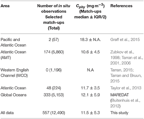
Table 1. Summary of in situ data.

The choice of phytoplankton types included in this computation, as well as the parameters used for the conversion to carbon, matches the modeling community approach as represented in Buitenhuis et al. (2012). The choice of phytoplankton types is such that phytoplankton types with diameter >2 μm are not taken into account. Furthermore, the choice of a mean carbon concentration per cell for each phytoplankton type does not permit accounting for any variations in size or cellular carbon spatially or temporally for each type of phytoplankton. To test our choice of carbon conversion parameters we compared direct measurements of C_phy with estimates computed using the conversion factors above. In samples from the AMT-22 (N = 15) (Graff et al., 2015), the slope of the regression between direct measurements of C_phy and computed C_phy, was 0.8 (r² = 0.6, p < 0.05). According to this result, the estimates of picoplankton C_phy in our dataset are significantly correlated with direct estimates of phytoplankton carbon, and could be an overestimate of direct observations of C_phy, which include nanophytoplankton, although a larger sample is required to support this conclusion.

2.2. In Situ and Satellite Match-up Selection

The in situ database described above was matched with merged ocean-color satellite data from the Ocean Color Climate Change Initiative (OC-CCI) (Sathyendranath et al., 2012). These merged products were used to maximize the possibility of finding matching in situ data as well as to use a set of common inputs to the different algorithms. The OC-CCI version 2 data had a daily sinusoidal projection (binned) and a 4 km spatial resolution. These satellite data were used as inputs for C_phy algorithms: total B from OC4v6, b_bp from the Quasi-Analytical Algorithm (QAA) v5 (a modification to v4 in Lee et al., 2002, 2007, but that does not include Raman scattering, Westberry et al., 2013; Lee and Huot, 2014). Second, the water class membership (Moore et al., 2001, 2009; Jackson et al., 2017).

The procedure for match-up selection was the same as that used for particulate organic carbon (POC) data (Evers-King et al., 2017). The day of year the in situ sample was collected was matched with the same day of year from the merged satellite products. Then all relevant data were extracted from a 3 × 3 pixel set with the sample location at the center. The number of valid data, within the 3 × 3 grid, and mean and standard deviation of the valid points were recorded for each computed C_phy product. The 3 × 3 grid was used to identify where sufficient satellite data were available. In this dataset only 11 matched points had 3 valid pixels or less. The C_phy algorithms were applied to the central pixel of the satellite matched up data. The match-up process reduced the sample size considerably. Further reduction came from depth-averaging (between 0 and 10 m) the C_phy profiles that matched the satellite data, and ignoring the deeper samples, leaving 647 data points. Finally, to remove outliers, the top and bottom 2 percentile were removed from the dataset, leaving N = 557 for the analysis. The geographical distribution of match-up database for the picophytoplankton carbon concentration, C_phy, is given in Figure 1. The match-up dataset usable for the algorithm comparison was only about 5% of the inital data (Table 1). It is worth emphasizing that the match-up data set has not been used for the calibration or development of most of the algorithms compared (see section 4).

FIGURE 1

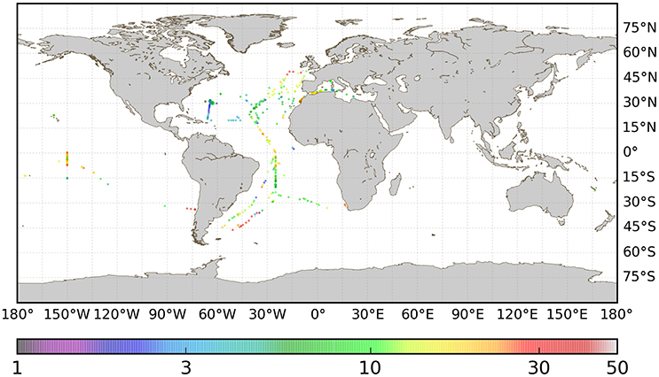
Figure 1. Geographical distribution of the match-up dataset (N = 557) used for algorithm testing. Color scale is concentration of picophytoplankton, C_phy in mg C m⁻³.

2.3. Ocean-Color Phytoplankton Carbon Algorithms

The following section describes the six algorithms compared in this exercise. All the phytoplankton algorithms were implemented using as input data the appropriate OC-CCI product for consistency and to isolate the effects of the different algorithms. Table 2 provides a comparison of the input data and the phytoplankton size range that is included in the outputs of each algorithm. These are important characteristics of the algorithms, required for the interpretation of the results. For phytoplankton carbon, C_phy in mg C m⁻³, six products were derived and they are briefly described in this section. According to their common characteristics, they can be grouped into chlorophyll-based, backscattering-based and allometric algorithms.

TABLE 2

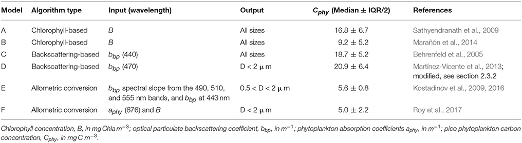
Table 2. Summary of C_phy algorithms main characteristics and median values predicted for the in situ match-up database (N = 557).

2.3.1. Chlorophyll-Based Algorithms

This family of algorithms use chlorophyll concentration as an input, B with units of mg Chla m⁻³. Chlorophyll in this study is obtained from OC-CCI merged dataset with the algorithm OC4v6, which is a band switching algorithm, mainly a fourth-order polynomial relationship between remote sensing reflectance in the blue and green bands. The two algorithms in this group use the same input and have a similar formulation, however, the assumptions made in their construction and hence their definition of C_phy are different. Algorithm A (Sathyendranath et al., 2009) was developed from an empirical relationship between in situ measurements of total particulate carbon and B. For this model, C_phy in Equation (2) below is an upper bound on the total phytoplankton carbon:

$\begin{array}{rc}{C}_{phy}=65\times B^{0.63}.& (2)\end{array}$

Algorithm B (Marañón et al., 2014) was also developed from an empirical relationship using in situ measurements of B, and not originally designed as an algorithm for ocean color applications. However, the estimates of total phytoplankton carbon originated from applying a conversion factor to microscope (counting cells with diameter, D > 5 μm) and flow cytometry (D < 10 μm) phytoplankton cell counts. This model is formulated in Equation (3) as:

$\begin{array}{rc}{C}_{phy}=62\times B^{0.89}.& (3)\end{array}$

Because of the difference in their definition of C_phy, Algorithm A and Algorithm B have been considered separately in our analysis. A priori, the expectation is that both chlorophyll-based algorithms, using total chlorophyll concentration as input data, will overestimate the picophytoplankton carbon from our in situ match-up dataset, since they are both designed to calculate total phytoplankton carbon, rather than just the picophytoplankton in our dataset. Further, it is also worth noting that the conversion factors used to compute phytoplankton carbon from cell abundance in Algorithm B are different to the ones used in our in situ match-up dataset.

2.3.2. Backscattering-Based Algorithms

Some semi-empirical algorithms use the (wavelength dependent) optical particulate backscattering coefficient, b_bp in m⁻¹, to estimate C_phy. The backscattering coefficient in this study is obtained from the OC-CCI merged dataset by applying the algorithm by the Quasi-Analytical Algorithm (QAA) v5 (a modification to v4 in Lee et al., 2002, 2007). In essence, the QAA first computes b_bp(555), from combining remote sensing reflectance at 555 nm with an empirical relationship between remote sensing reflectance ratios and the total absorption coefficient and the backscattering of pure seawater (modeled). Then, to propagate the b_bp(555) at other wavelengths, the algorithm uses a band ratio (again blue to green bands) to compute the backscattering spectral slope. The same QAA b_bp product is used for both backscattering based C_phy algorithms, but at different wavelengths. Algorithm C (Behrenfeld et al., 2005) uses b_bp(443) as an input:

$\begin{array}{rc}{C}_{phy}=13000\times (b_{bp}(443)-0.00035).& (4)\end{array}$

As this algorithm was developed from MODIS-Aqua (Moderate Resolution Imaging Spectroradiometer) ocean-color data, and 443 nm is a native OC-CCI band, no spectral adjustment is therefore needed. However, it is worth noting that the algorithm was developed originally using the GSM algorithm (Garver and Siegel, 1997; Maritorena et al., 2002; Siegel et al., 2002), but in this test, the b_bp input come from the QAA algorithm. The C_phy derived with this algorithm includes all the phytoplankton size ranges. Algorithm D (Martínez-Vicente et al., 2013) is another semi-empirical algorithm, developed from the relationship between in situ flow cytometry-based carbon and b_bp(470), but is included in the comparison with some changes. The first modification was to re-compute the coefficients in the original equation by using the same computation of picoplankton as the one used in this work, which meant ignoring the nanoeukaryotes, cryptophytes and coccolithophorids contributions to the picoplankton carbon and use the same carbon to cell conversion factors as in this study (i.e., those of MAREDAT; Buitenhuis et al., 2013). This re-calculation led to lower (pico)phytoplankton carbon estimates which were, on average, 27% less than the published values of phytoplankton carbon (from pico- and nano-plankton) used in Martínez-Vicente et al. (2013). When the new picophytoplankton C_phy estimate was used with the original in situ b_bp data, the resulting fit was:

$\begin{array}{rc}{C}_{phy}=18000\times (b_{bp}(470)-43*10^{-5}),N=70.& (5)\end{array}$

This equation explains considerably less variance in the observed data (r² = 0.4) than the r² of 0.89 reported in the original work. However, it makes the definition of C_phy by this model directly comparable to the in situ data. The second modification was to adjust the backscattering coefficient wavelength from the available value, 490 to 470 nm. To do so, the spectral slope of the b_bp from the OC-CCI data was obtained by doing an ordinary least squares fit to the log₁₀ transformed data and calculated the new b_bp(470) needed for Equation (5).

2.3.3. Allometric Type Algorithms

These algorithms belong to a family of algorithms that use optical properties to compute phytoplankton size structure and then convert it into biomass (Mouw et al., 2017). Algorithm E (Kostadinov et al., 2016) retrieves the absolute and fractional phytoplankton carbon biomass in three phytoplankton size classes (or, approximately equivalent − phytoplankton functional types) − picophytoplankton (0.5–2 μm in diameter), nanophytoplankton (2–20 μm) and microphytoplankton (20–50 μm). The algorithm uses retrievals of the particle size distribution (PSD) to estimate particle volume. Note that the PSD is estimated for all particles in suspension in the water. Particle volume is then converted to carbon concentrations using a compilation of existing allometric relationships between size and carbon content of phytoplankton cells (Menden-Deuer and Lessard, 2000). Derived carbon concentration is then divided by 3 to estimate the living phytoplankton carbon fraction. The PSD retrievals themselves are based on a PSD algorithm (Kostadinov et al., 2009), which relates the spectral slope and magnitude of the backscattering coefficient spectrum to the underlying parameters of an assumed power-law PSD, via look-up tables (LUTs) constructed using Mie theory modeling. In the implementation used here, the input backscattering spectrum comes from the standard QAA products of the OC-CCI dataset, which are derived using Lee et al. (2002) algorithm, as summarized above. This is different from the original implementations (Kostadinov et al., 2009, 2016), where the Loisel and Stramski (2000) algorithm was used to retrieve spectral b_bp. The PSD parameters retrieved are the power-law slope (ξ) and the scaling parameter (i.e., differential particle number concentration at a reference diameter of 2 μm, N_o, [m⁻⁴]). Kostadinov et al. (2016) applied an empirical correction to the PSD scaling parameter N_o obtained from the model LUT, to improve absolute phytoplankton carbon concentration estimates.

A further allometry-based method, Algorithm F (Roy et al., 2017), uses chlorophyll concentration and the absorption coefficient of phytoplankton at 676 nm, a_ph(676), to compute phytoplankton carbon. In this algorithm, the exponent of the phytoplankton size spectrum (ξ) is first computed from the specific-absorption coefficient of phytoplankton at 676 nm, $a_{ph}^{*}(676)$ using a method developed by Roy et al. (2013). This algorithm uses as input B from OC4v6 and a_ph(676) from QAA, both standard products in the OC-CCI dataset. The estimated exponent of the size spectrum ξ and the allometric relationships between the cellular content of phytoplankton carbon (C_cell) and cell volume (V_cell) reported by Menden-Deuer and Lessard (2000) are then used to compute the concentration of phytoplankton carbon (C_total, in mg C m⁻³) contained in the cells within any specified diameter range. To do so, the allometric parameters corresponding to the mixed populations of phytoplankton are derived from the allometric relationships found for individual groups of phytoplankton, as reported in Menden-Deuer and Lessard (2000), by performing linear regression. The derived allometric relationship is used then to compute the magnitude of the carbon-to-chlorophyll ratio (χ), using the derived allometric expressions for the concentrations of chlorophyll and phytoplankton carbon, C_total. Finally, phytoplankton carbon for the specified size range is computed as the product of χ and satellite-derived chlorophyll concentration (for more details see Roy et al., 2013, 2017). The allometry-based algorithms E and F were used to compute picophytoplankton concentration within a diameter range 0.2–2.0 μm, which is directly comparable with the size range included in the matching in situ database.

In summary, each method is thus based on a satellite measurement that provides underlying variability in the resulting C_phy (reflectance ratio or analytically-derived backscatter) which is then combined with selected empirical relationships that scale those measurements to C_phy (using either linear or non-linear relationships and sometimes including more than one step, such as via B). The strength of this study lies in the use of the OC-CCI satellite dataset as a common source of inputs for all the algorithms, which removes sources of uncertainty from other parts of the satellite processing. A limitation, however, comes from the differences in the definition of the C_phy for each algorithm (Table 2). It is expected that the algorithms which compute total C_phy (i.e., Algorithms A, B, and C) will be most comparable to the in situ data when the contribution to the phytoplankton Carbon by nano and picoplankton is not significant.

2.4. Statistical Metrics and Their Contribution to the Study

Ranking of algorithms according to their performance is a classic exercise for the ocean-color community, that has evolved from comparisons of chlorophyll algorithms (O'Reilly et al., 1998) to more complex and comprehensive approaches recently (Brewin et al., 2015; Kostadinov et al., 2017). Typically, a battery of statistical metrics is used to construct an index of overall performance against a set of matched data with in situ observations (Brewin et al., 2015). In this exercise, however, we do not use a scoring system to rank algorithms, since one of the aims of this work is to provide an overall idea of the current accuracy of the phytoplankton Carbon product from a group of algorithms. The Kolmogorov-Smirnov test for normality of the in situ match-up data showed a significant deviation from normality for log₁₀ transformed and un-transformed data and the residuals (p < 0.001). Therefore, statistical metrics that assume normality would be less reliable. For completeness, the statistical tests were computed for log₁₀ transformed data, using parametric tests; and for un-transformed data, using non parametric, rank-based, statistics. Statistical metrics computed were:

• Pearsons correlation coefficient for log₁₀ transformed data, and Spearman's correlation for un-transformed data (r_p and r_s respectively),

• Root mean square differences (RMSD, Ψ),

• Signed average bias (δ),

• Median absolute percentage deviation between predictions and observations, (MAPD in %) was an estimate of bias and precision was estimated as the interquartile range (IQR) of the absolute percentage deviation for the untransformed data.

• Center pattern root mean square differences for log₁₀ transformed and un-transformed data (Δ), and

• Slope and intercept (S, I) from a Type-II linear regression (Reduced Major Axis) for log₁₀ transformed and un-transformed data.

To provide an indication of the stability of the statistics and to compute confidence intervals on them, bootstrapping (Efron, 1979; Efron and Tibshirani, 1993) with random re-sampling and replacement was used to construct 1,000 different datasets from which confidence intervals were computed for some of the statistical metrics above. These metrics were computed for all the algorithms tested against the match-up dataset as a whole and, in adition, they were also computed after segregating the match-up dataset according to the dominant water class at the central match-up pixel. Because of the nature of the ocean color CCI satellite data and the C_phy algorithms, it is expected that algorithm performance will degrade toward more turbid environments (water classes 8 and over). Furthermore, the statistical results per water class provided a measure of dispersion of the phytoplankton Carbon product among algorithms, describing in which optical environments the algorithms show greater agreement. The statistics per water class were used to produce uncertainty maps (RMSD and bias). To generate the uncertainty maps, the optical class memberships at each pixel, and the per-class uncertainty values for each class were used to produce a weighted average uncertainty value for the pixel, with the weighting function being provided by the class membership. This is the method followed by the OC-CCI and described fully in Jackson et al. (2017).

3. Results

3.1. Distribution of in Situ Data and Accuracy of Algorithms

The sources and geographic distribution of the in situ data, as well as the corresponding median values of the picophytoplankton carbon data are summarized in Table 1. The spatial distribution of the match-ups (Figure 1) shows their limited coverage of the oceans, with most of the data (71%) located in the Northern Hemisphere and from the Atlantic Ocean. The overall median value of C_phy from the match-up database was 11.7 ± 5.3 mg C m⁻³ (median ± IQR/2), with values ranging from 1.7 to 60.2 mg C m⁻³. As a comparison, chlorophyll concentration (B) from the coincident satellite data was 0.12 ± 0.08 mg Chla m⁻³, ranging from 0.01 to 3.53 mg Chla m⁻³. The median values of C_phy from the algorithms applied to the matching data (Table 2) were not significantly different to the C_phy in situ (Mann-Witney test, N = 557, p < 0.05). Relative frequency histograms of these data (Figure 2) however, show some bias. The peaks of the histogram of the chlorophyll-based algorithms (Algorithms A and B) were closest to the in situ; the backscattering-based models (Algorithms C and D) were double the median of in situ and allometric algorithms (Algorithms E and F), were half the in situ median value (Figure 2). The distribution spread of chlorophyll-based algorithms were about the same or wider than the in situ (C.V. between 40 and 56%), with backscattering and allometric algorithms having narrower distributions (C.V. lower than 30%).

FIGURE 2

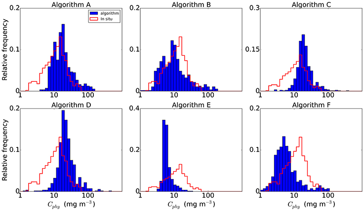
Figure 2. Relative frequency distribution of C_phy of the in situ data compared with the algorithms outputs. Note change in the scale of y-axis for Algorithms C and E.

Figure 3 shows the results from the algorithm estimates of C_phy against in situ derived estimates of C_phy and the relevant statistical metrics are in Table 3. All the algorithms showed different predictions of C_phy, but as expected, there were commonalities among models that shared the same formulation. For example, both chlorophyll-based algorithms (Figures 3A,B) presented an elongated cloud with a weak but positive (~0.6) and significant correlation with in situ data, and stayed mostly along the 1:1 line, with slopes close to 1; whereas both backscattering-based algorithms (Figures 3C,D), had weaker correlations (~0.4) and, although the slopes where also close to 1, the data cloud does not capture the lower C_phy measurements. Contrary to the other two groups of algorithms, the allometric-based do not share a formulation, hence their results (Figures 3E,F) differ significantly among them.

FIGURE 3

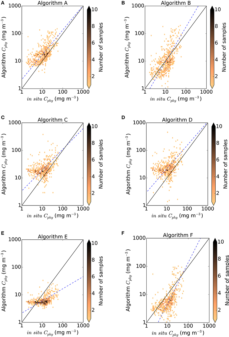
Figure 3. Density plot of in situ vs. algorithm C_phy from the match-up database (N = 557). Black solid line is the 1:1 line and blue dashed line is the Type II linear regression (Reduced Major Axis) fitted to the log₁₀ converted data. (A) Sathyendranath et al. (2009), (B) Marañón et al. (2014), (C) Behrenfeld et al. (2005), (D) Martínez-Vicente et al. (2013) modified, (E) Kostadinov et al. (2009, 2016), (F) Roy et al. (2017).

TABLE 3

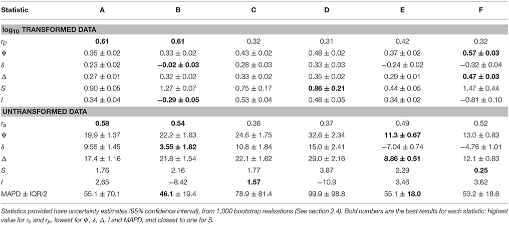
Table 3. Summary of statistics of algorithm performance (algorithms A–F, columns) for log₁₀ and untransformed data (N = 557).

The statistical metrics (Table 3) provide a range of values among the algorithms tested, showing that there is not a clearly superior performance of a single algorithm on all metrics. The bias (δ) ranged from 3.5 mg C m⁻³ for Algorithm B (Marañón et al., 2014) to 15 mg C m⁻³ for the Algorithm D (Martínez-Vicente et al., 2013) as modified in this work. Chlorophyll and backscattering based algorithms had a positive bias, less than 15 mg C m⁻³, whereas allometric algorithms had a negative bias, less than 7 mg C m⁻³. The un-biased RMSD (Δ), which gives an idea of the dispersion of the predictions, ranged from 8.9 mg C m⁻³ for Algorithm E (Kostadinov et al., 2016) to 29 mg C m⁻³ for Algorithm D, (Martínez-Vicente et al., 2013) as modified in this work. The lowest median absolute percentage difference (MAPD), a measure of accuracy, for the untransformed data was for Algorithm B (Marañón et al., 2014), in agreement with the bias indicator for log and non-log transformed data. The inter-quartile range of the MAPD (IQR), a measure of precision of the algorithm, was lowest for Algorithm E (Kostadinov et al., 2016), and coincided with another indication of dispersion (Δ) in the non-log statistics, but differed for the log-transformed data.

Overall, chlorophyll-based algorithms had higher correlation and indicators of lower bias (i.e., δ, MAPD), whereas allometric algorithms had indicators of lower dispersion (i.e., Δ, IQR of MAPD). Between algorithms, there was a factor 4 of difference between the maximum and minimum predictions from the algorithms for all matchups pooled together as a median (i.e., the median of the fractional difference between the minimum and the maximum predictions by the algorithms in each match-up point).

An additional way to assess model performance is to study their emergent properties (de Mora et al., 2016). Here we have compared the in situ and the algorithm derived C_phy to the chlorophyll concentration, B (standard OC4v6 OC-CCI-product) for the match-ups (Figure 4 and Table 4), to investigate the behavior of the C_phy:B ratio. Figure 4A displays the positive correlation between the satellite derived B (for the whole of the phytoplankton assemblage) and the in situ derived C_phy for the picophytoplankton fraction only, over more than two orders of magnitude of chlorophyll concentration. Because of the mismatch between the particle assemblage in B and C_phy, the overall values reported for the C_phy:B ratio are smaller than they would be if the ratio had been derived from B for picoplankton only. However, with a median value of 91 mg C mg Chla⁻¹, the in situ C_phy-to-satellite-B-ratio falls within or close to observed values in oligotrophic areas. For instance, Sathyendranath et al. (2009) reported average values of this ratio greater than 100 mg C mg Chla⁻¹ for prymnesiophytes, cyanobacteria and Prochlorococcus sp. Direct observations of pico and nano plankton carbon in the Northern and Southern Atlantic gyres produced carbon-to-chlorophyll ratio estimates, on average, of 106 and 190 mg C mg Chla⁻¹, respectively (Graff et al., 2015). Marañón et al. (2014) also reports values in the range of 80–117 mg C mg Chla⁻¹ for oligotrophic regions. Therefore, the C_phy:B ratio used as reference in this study compares well with existing observations reported in the literature, despite the mismatch between the phytoplankton assemblages considered. These data are repeated as the background of the other panels in Figure 4 for reference along with their corresponding regression line. Algorithms A and B are chlorophyll-based, therefore their predictions fall on the line of the equations used, respectively Equations 2, 3 in Figures 4B,C. Their predictions are close to the in situ data cloud and the resulting median phytoplankton carbon-to-chlorophyll ratio encompass the in situ reference value, Algorithm A providing an upper limit, as expected from the assumptions made in its construction. Backscattering-based algorithms (Algorithms C and D, in Figures 4D,E, respectively) overestimate the C_phy:B reference relationship, specially at the lower concentrations of chlorophyll, and produce median phytoplankton carbon-to-chlorophyll ratio values up to two times greater than the reference. However these algoritms capture some of the variability around the prediction line, which is in the same order of the in situ data. Algorithms using inherent optical properties with allometric conversions (Algorithms E and F, in Figures 4F,G, respectively) underestimate the reference C_phy:B reference relationship, with Algorithm E showing a narrower distribution of data points than Algorithm F.

FIGURE 4

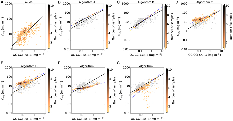
Figure 4. Density plot of covariance between OC-CCI standard chlorophyll product and C_phy from the match-up database (N = 557). (A) In situ C_phy, (B) Sathyendranath et al. (2009), (C) Marañón et al. (2014), (D) Behrenfeld et al. (2005), (E) Martínez-Vicente et al. (2013) modified, (F) Kostadinov et al. (2009, 2016), (G) Roy et al. (2017). Blue dashed line is the Type II linear regression (Reduced Major Axis) fitted to the log₁₀ converted data. Black solid line is the regression line between chlorophyll and in situ for comparison with the regressions by the algorithms. For comparison, data in (A) are repeated (gray) in the other panels.

TABLE 4

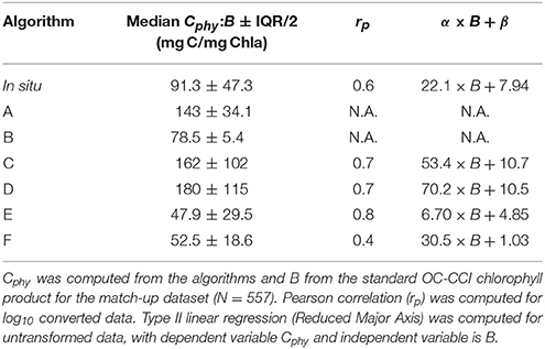
Table 4. Summary of statistics for the C_phy to B relationships.

The in situ C_phy dataset is representative only of a fraction of the particle population (picophytoplankton). However, its geographical distribution, the median C_phy concentrations and carbon-to-chlorophyll ratios derived from this dataset are in agreement with existing observations in oligotrophic oceanic conditions. Taking into account this charcteristic of the dataset, the overall performance of the algorithms was on the low side, with chlorophyll-based algorithms producing slightly lower bias and allometric algorihms slightly lower dispersion. Among algorithms there was a median dispersion of a factor 4 between minimum and maximum predictions. The algorithms were also tested on their ability to produce realistic a C_phy:B ratio, which again highlighted great dispersion in predictions among and within algorithms types. Arguably, part of the dispersion in the statistical results may have arised from the fact that the in situ C_phy dataset is representative only of a fraction of the particle population (i.e., picophytoplankton). Therefore if we limited the study to the optical cases where picophytoplankon is expected to dominate the phytoplankton carbon pool and the chlorophyll content, we would expect an improvement on the results from the algorithms. In the next part of this study we present results obtained from segregating the data into optical water types.

3.2. Algorithm Comparisons for Individual Optical Water Types

An optical water class, in this context, is defined by a mean remote sensing reflectance spectrum representative of particular optical characteristics, i.e., an end-member spectrum. Each extracted satellite pixel coinciding with a match-up in situ data has contributions from the different end-members in different proportions. The water class contributing with the largest proportion to the pixel water class membership is classed as belonging to that water class (Jackson et al., 2017). The geographic locations of the match-up points per water class and the number of observations per class are shown in Figure 5. There was a good correspondence between the geographic location of the optical water types (note that the classes are numbered such that i = 1 is the most oceanic type and i = 14 the most coastal type) in Figure 5A and the C_phy concentrations (Figure 1), such that the higher-numbered optical classes tend to be representative of higher concentrations of phytoplankton carbon. The majority of the data (63%), though can be classed as representative of an oligotrophic environment (i 1 to 6, B < 0.15 mg Chla m⁻³). A boxplot summary of the descriptive statistics per optical water class per algorithm is provided (Figure 6). Table 5 summarizes the median C_phy values highlighting a steady increase from oceanic to coastal waters, except for i = 13, which only has N = 5 observations, and is hereafter discarded from the analysis. The magnitude and the increase of the picophytoplankton carbon is in agreement with oceanic and coastal data (Tarran et al., 2006). For instance, using the current carbon conversion parameters on existing abundance data (Tarran and Bruun, 2015), C_phy median in the coastal area of the Western English Channel is 12.1 ± 6.1 mg C m⁻³ (N = 68).

FIGURE 5

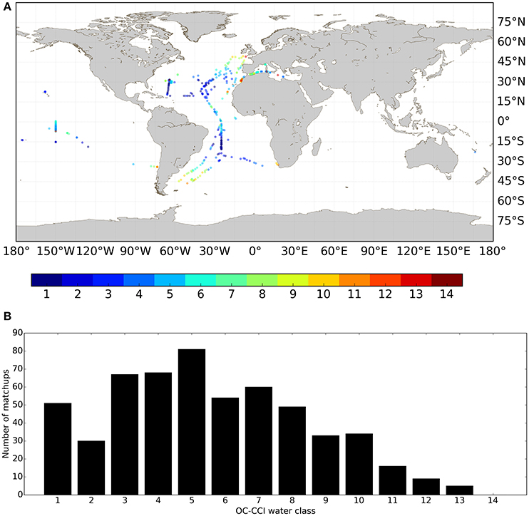
Figure 5. Distribution of the C_phy from the match-up dataset per optical water class. (A) Geographical distribution. (B) Number of data per optical water class.

FIGURE 6

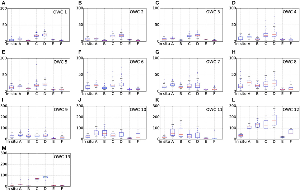
Figure 6. Box-whiskers plots of C_phy (in mg C m⁻³) for the optical water classes (OWC in the figures) 1–13 corresponding to sub-figures (A–M) respectively. The output of each algorithm (A–F) is compared to the in situ measurement for each optical water type. Note change of vertical scale in plots (I–M), corresponding to optical water classes greater than 9. Box, Inter Quartile Range (IQR); red line, median; whiskers, ±1.5×IQR.

TABLE 5

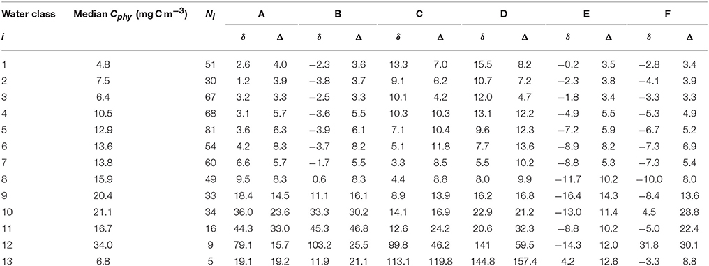
Table 5. Median C_phy from in situ matchups and non-log average bias (δ) and un-biased RMSD (Δ) of the different algorithms (algorithms A–F, columns headers) per water class number (i) in mg C m⁻³, alongside with the number of observations per water class (N_i).

Algorithm performance per water class was quantified by the signed bias (δ) and the center-pattern RMSD (Δ) (see Table 5 and Figure 7). These statistical indicators of performance improved by limiting the analysis to oligotrophic waters (i 1 to 6) as expected: bias, δ, was similar or lower than those obtained when considering all data, for all the algorithms (section 3.1, Table 3). Center-pattern RMSD, Δ an indicator of precision, was, on average, half that when considering all data, indicating decreased noise in the retrieval for all algorithms (for non-log results, section 3.1). Chlorophyll-based algorithms had, on average, similar δ and Δ to the allometric-based algorithms, with back-scattering based algorithms producing higher bias and higher Δ values.

FIGURE 7

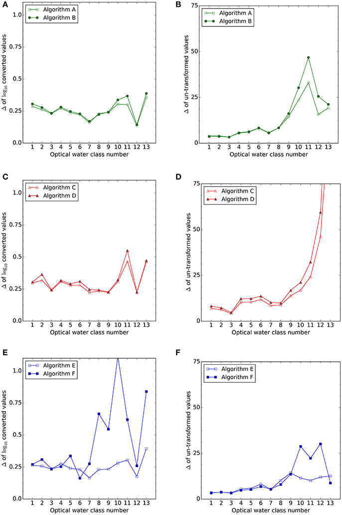
Figure 7. Center pattern root mean square deviation (Δ) for log₁₀ (A,C,E) and non-transformed (B,D,F) data from the C_phy match-up dataset per optical water class. Out of scale from the plot in (D) Algorithm C for water class 13 has Δ = 120 mg C m⁻³; Algorithm D for water class 13 has Δ = 157 mg C m⁻³. (E) Algorithm F for water class 10 has Δ = 1.12 mg C m⁻³.

Mesotrophic waters (0.15 < B < 0.7 mg Chla m⁻³, or optical water classes 7–10) comprise 32% of data. With respect to the results obtained for all data available (section 3.1), the chlorophyll based algorithms had an increased δ, whereas Δ was similar. Backscattering-based algorithms had higher uncertainties than chlorophyll-based algorithms in the more turbid waters (high optical class numbers) in the untransformed data (Figure 7D). Bias increased for all of the algorithms for these water classes except for Algorithm E, which remained negative and relatively constant at −60%. However, the results for mesotrophic and more turbid waters, should be taken with caution as the use of in situ C_phy data comprising only picophytoplankton is more problematic in these waters.

The in situ median C_phy:B ratio by optical water class were also compared to the median C_phy:B ratio from the algorithms (Figure 8). The in situ data (solid gray line and error bars) is repeated as a reference throughout Figure 8, showing that for i from 1 to 6 (oligotrophic waters), the range of variation is narrow (106 to 165 mg C mg Chla⁻¹, median 133 mg C mg Chla⁻¹) and error bars are overlapping among the optical water classes 1 to 6. For mesotrophic waters (i from 7 to 10), there was a decreasing tendency of the in situ C_phy:B ratio.

FIGURE 8

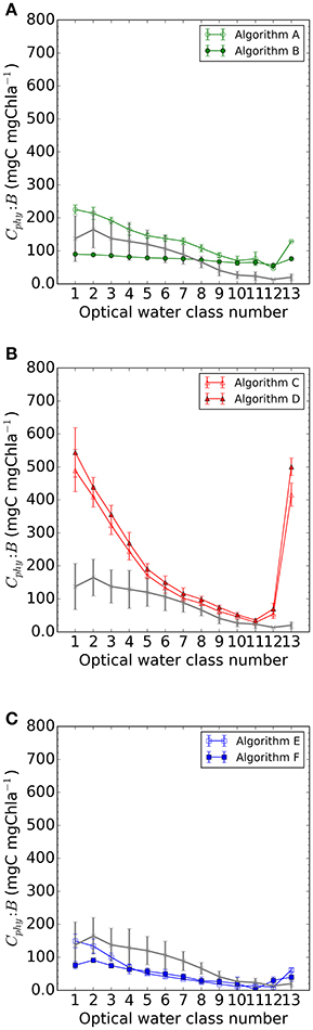
Figure 8. Median C_phy:B for each optical water class in the match-up dataset per type of algorithm: (A) chlorophyll-based algorithms A and B; (B) backscattering-based algorithms C and D and (C) allometric algorithms E and F. Error bars are the IQR/2 for the water class. Gray line and error bars in all sub-figures are obtained from the in situ dataset.

The analysis of the algorithm predictions of the C_phy:B ratio focusses on the optical water classes 1 to 6, where C_phy and B are expected to describe the same phytoplankton assemblage. Essentially, the behavior observed for the C_phy is also repeated here. Algorithm A was an upper limit to the C_phy, it is also an upper limit to C_phy:B ratio, which decreases with increasing optical water class number (Figure 8A). Algorithm B shows relatively little variation of the median C_phy:B ratio for the optical water classes of interest and beyond (i > 6). Backscattering-based algorithms, Algorithm C (Behrenfeld et al., 2005) and Algorithm D (Martínez-Vicente et al., 2013), showed also decreasing median C_phy:B ratio with increasing water class number, with large overestimations with respect to the in situ C_phy:B ratio at the clearest waters. The allometric-based algorithms, Algorithm E (Kostadinov et al., 2016) and Algorithm F (Roy et al., 2017), were generally predicting lower than observed C_phy, and also predicted lower median C_phy:B ratios. However, both algorithms had a decreasing tendency for the median values with increasing turbidity (or water class number, in this study), with Algorithm E being closest to observations for i from 1 to 3.

Finally, Figure 9 shows an example of the C_phy product from algorithms A to D using the OC-CCI monthly product from May 2005. All algorithms reproduce the broad patterns that would be associated with C_phy i.e., increased values in high-chlorophyll areas (upwelling sites and coastal regions) and lower concentrations in the gyres, however the salient point of this Figure is the large differences in predictions among the algorithms, as expected from the statistical results.

FIGURE 9

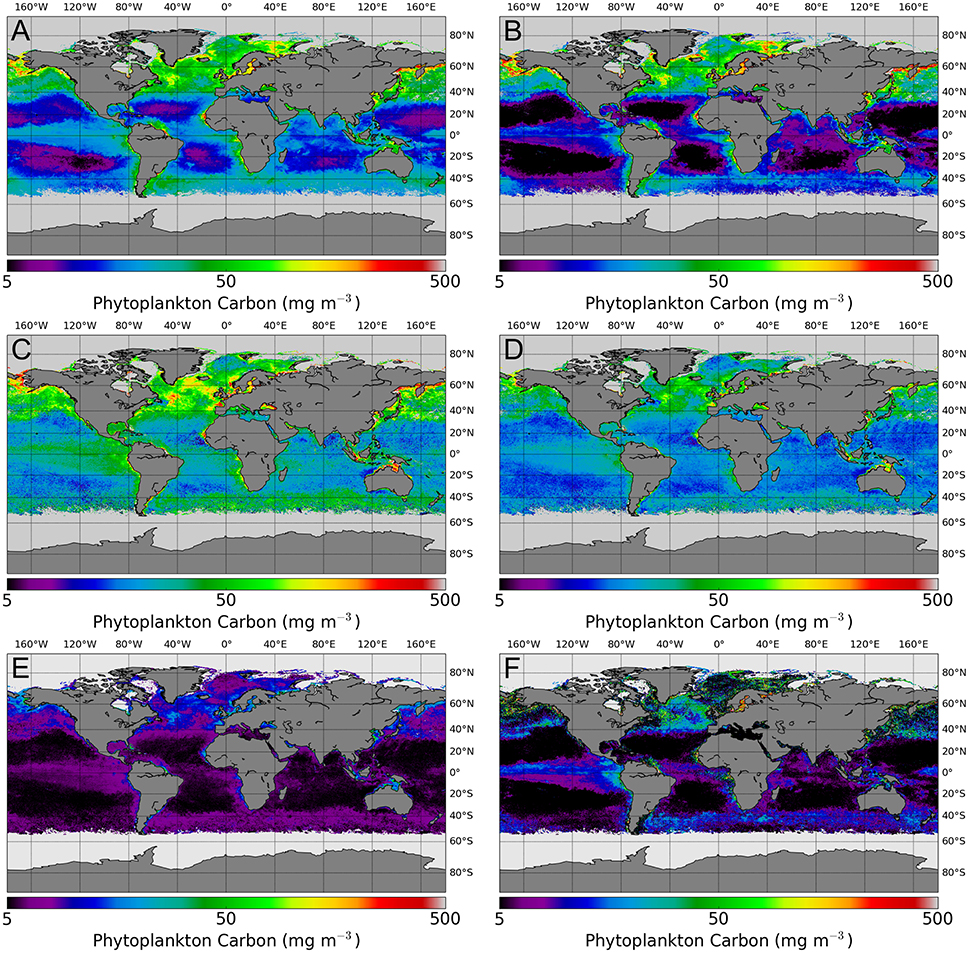
Figure 9. An example of the C_phy product for May 2005, estimated using each of the algorithms (A–F) applied to the monthly OC-CCI data. Black color in the gyres indicate values close or below 5 mg C m⁻³, light gray indicates invalid retrieval or unavailable input data.

4. Discussion

4.1. The Picophytoplankton C Match-up Dataset

This study has compiled a large in situ database of picophytoplankton carbon, building on a combination of a substantial pre-existing effort by the modeling community (the MAREDAT data) and long time series observation programmes in the open ocean (Atlantic Meridional Transect, AMT). The ambition is to see this dataset growing with time, as new data are incorporated.

There are a number of advantages and limitations for this dataset with respect to its use for algorithm testing and validation. An advantage is that only a small fraction of the data have been used for the development of any of the algorithms tested here. Algorithms A, B, C, and E are completely independent of the match-up dataset. Algorithm D as implemented by Martínez-Vicente et al. (2013), was developed using a small subset of the new database, N < 70, but the subset included nanoplankton. Algorithm F used MAREDAT for testing algorithm performance, but not for its development. So the data for the validation presented here are mostly independent of the data used in the construction of algorithms. The geographic distribution of the match-up database, though largely limited to the Atlantic, with some additional points from the Pacific, does cover a variety of oceanic regions. It is a purpose-built database for satellite validation studies, and therefore, only an average of the matching data in the top 10 m have been selected for convenience.

However, the dataset also has limitations. One of them is that it is only composed of picophytoplankton: though they are important contributors to the open-ocean phytoplankton biomass, picophytoplankton form a decreasing proportion of the phytoplankton biomass in more productive waters, where larger cells tend to become more important (Marañón et al., 2012; Marañón, 2015). One interesting avenue would be to expand the database with other phytoplankton groups (Buitenhuis et al., 2013; Sal et al., 2013). Nanoplankton can also be counted using flow cytometry, and microphytoplankton groups counted using microscope or automated image processing (Sosik and Olson, 2007; Álvarez et al., 2012), but the relationship between carbon and abundance becomes more variable for larger and more irregularly-shaped phytoplankton (Moberg and Sosik, 2012; Saccà, 2016).

Because the data are confined to the surface layers, they may also be adversely affected by underestimation of Prochlorococcus sp. abundance by flow cytometry because of extremely low fluorescence per cell (Partensky et al., 1996; Heywood et al., 2006). Furthermore, by limiting our dataset to the top 10 m, we have precluded the possibility of testing any potential impact that the vertical structure in the first optical depth might have on algorithm performance. Examples exist in the literature where the depth variations in particulate organic carbon been taken into account (Duforêt-Gaurier et al., 2010), and this may be an avenue worth exploring also for phytoplankton carbon algorithms.

Finally, the conversion of abundance to carbon using estimates from the laboratory could cause errors in the computed C_phy in the field, if the laboratory estimates do not hold under natural environmental conditions. These factors can vary with physiological state and with depth (Casey et al., 2013) and have been discussed previously (Buitenhuis et al., 2012; Martínez-Vicente et al., 2013). It is important to highlight that in this study we have used indirect estimates of phytoplankton carbon (through cell counts and cell size) only because of the lack of direct measurements. However, methods for direct quantification of C_phy have recently become available (Graff et al., 2012; Casey et al., 2013) and the expectation is that there will be more direct C_phy data available in the future.

Limiting the study to the optical water classes where the composition of the phytoplankton assemblage is expected to be dominated by picoplankton (i 1 to 6, B up to 0.15 mg Chl m⁻³) median values of C_phy and C_phy:B ratio matching the literature (Marañón et al., 2001; Marañón, 2015), were obtained, and the algorithms results showed more stability and less dispersion. However, some algorithms displayed significant differences which are discussed hereafter.

4.2. Algorithm Comparison by Type: Chlorophyll Based, Backscattering Based and Allometric

The algorithms presented here were broadly classified into three classes: chlorophyll-based, back-scattering based and allometric. In the results presented here, it is evident that algorithms based on similar approaches perform alike. So it is worth examining each of these approaches in some detail, to explain the differences observed in the results for oligotrophic waters.

The two chlorophyll-based algorithms were designed to consider all the phytoplankton groups: Algorithm A (Sathyendranath et al., 2009) provides an upper limit to the phytoplankton contribution to the total particulate carbon pool and Algorithm B (Marañón et al., 2014) is based on phytoplankton carbon computed from flow-cytometric data supplemented with microscopic counts for larger phytoplankton. Yet, when compared with only one fraction of the total phytoplankton pool (the picophytoplankton in this study), the results are similar, with Algorithm A slightly overestimating and Algorithm B slightly underestimating in situ C_phy. Algorithm A was designed as the upper limit to the phytoplankton carbon, hence this result is as expected. Algorithm B was computed using a similar conversion method between cell count and carbon concentration to the one used in this study, but with different conversion coefficients. We speculate that a possible reason for the difference observed between the predicted C_phy by Algorithm B and the in situ C_phy could be found in the differences in conversion between cell counts and carbon. Production of datasets with consistent conversion factors would help eliminate this source of discrepancy.

Differences in results are greater with the backscattering-based algorithm, which produced overestimation of C_phy and greater dispersion statistics than the other algorithms. Because it has been verified in situ that b_bp increases with pico and nano plankton carbon (Martínez-Vicente et al., 2013; Graff et al., 2015), the degradation of results may be linked to the backscattering input from the algorithm. Algorithm C equation was derived using the GSM algorithm for obtaining a relationship between the backscattering coefficient and the B. It has been found in situ, that at low B there may be an overestimation of the b_bp by using this satellite-derived relationship (Huot et al., 2008; Antoine et al., 2011; Brewin et al., 2012), yet in situ data also have shown overestimation of backscattering by the QAA algorithm (Behrenfeld et al., 2013). It has been found recently, that Raman scattering plays a role in the discrepancy of the retrievals of the backscattering coefficient in very clear waters from satellite (Westberry et al., 2013), causing an overestimation in backscattering. This effect of Raman scattering has been only identified recently (Lee and Huot, 2014), and was not incorporated in the QAA version used for the production of the OC-CCI version 2 data used for this study, but can be analytically corrected (McKinna et al., 2016), and future versions of the OC-CCI dataset will address this issue.

While validation of the OC-CCI chlorophyll product has been performed intensively in Atlantic oligotrophic waters and showed low error statistics (Brewin et al., 2016), investigations to improve the validation of b_bp and to understand better the relationships of b_bp with particles in oligotrophic areas are still required (Brewin et al., 2015). At a fundamental level, backscattering is dependent on the refractive index of the cells, their abundance and size, whose interplay is not yet fully understood. But in addition to phytoplankton, other particles (e.g., detritus) are known to contribute to the backscattering signal, and their variability relative to phytoplankton could potentially contribute to the discrepancies observed in this study.

Algorithm E used in its original formulation an inversion model to retrieve the backscattering spectral slope (Loisel et al., 2006) that is different from the one used in this comparison as input (i.e., QAAv5). The QAA used here invoked a band ratio to solve for the backscattering spectral slope, and this may account for at least part of the observed tighter coupling between B and Algorithm E. Algorithm E provides consistently low Δ values across the water classes, although it underestimates the in situ data systematically. This may be pointing to a need to re-adjust the size scaling parameter (like N_o), the empirical correction for which is now based on a rather limited in situ validation data set (Kostadinov et al., 2016). Ultimately, a better optical closure is needed between modeled and observed backscattering spectra, and a better understanding of the underlying particle assemblages, their refractive indices, and their relative contributions to the backscattering coeffient. It remains to be validated if at more productive waters, the prediction of low C_phy (from Algorithm E picophytoplankton fraction) remains valid, whereas the current in situ dataset showed an increase (Table 5).

Algorithm F was similar to algorithm E in all water classes except for water classes 8 to 11, where the uncertainty is almost double compared with the rest of the algorithms, pointing perhaps to a vulnerability to uncertainties in the a_ph(676) retrieval in these waters. More accurate estimates of phytoplankton carbon by Algorithm F would possibly require improving the retrievals of the input a_ph(676) values, especially in high-chlorophyll waters.

5. Conclusions and Future Work

Further work is required to extend the in situ dataset to include additional phytoplantkon sizes to evaluate if uncertainties can be reduced in the product by including larger phytoplankton to capture phytoplankton dynamics at wider scales. Despite the limitations of the in situ data used, it has been shown that where chlorophyll concentrations are less than 0.15 mg Chla m⁻³, chlorophyll-based algorithms provide the best estimates of C_phy, allometric-based algorithms consistently underestimate C_phy and backscattering-based algorithms, can produce large overestimations of C_phy, at least for the particular case of back-scattering data, provided using the QAA algorithm, as implemented in OC-CCI version 2.0. To improve back-scattering products from satellites, fundamental optical work on explaining the relationship between the b_bp and particles in oligotrophic areas is still needed. Satellite-based phytoplankton carbon product, once validated to a level that meets user requirements, and in situ datasets, similar to the one presented here, will be useful for validation of marine ecosystem and biogeochemical models at a wider scale (Dutkiewicz et al., 2015).

Data Available

The C_phy data, computed from in situ phytoplankton counts, and the matching C_phy data, computed from different algorithms using OC-CCI version 2.0 satellite data, can be obtained from http://www.zenodo.org with 10.5281/zenodo.1067229.

Author Contributions

VM-V: Lead writer, collation of in situ database, statistical analysis and production of code for match-up evaluation. HE-K: Production of code for satellite processing and match-up extraction, and writer. RB: Provision of code for statistical analysis based on OC-CCI methodology. TJ: Provision of code for calculation of per optical water class uncertainties, based on the OC-CCI methodology. GD: Provision of in situ data. AH: Perspectives on ecosystem modeling. SR: algorithm provider, input in statistical analysis/interpretation. RR and HK: Review of the in situ database. TK and EM: Algorithm providers. JG: Data provider. GT: Data provider. TP: Project leader, scientific advice. SS: Co-lead development of the concept, work plan and guidance. All authors reviewed and provided comments on the draft manuscript.

Funding

Several authors (VM-V, SS, TP, SR, HE-K, GD, AH, RR, and HK) were supported by POCO, which is a project funded by the European Space Agency (ESA) under the program of Science Exploitation of Operational Missions (SEOM) following Contract: 4000113692/15/I-LG. This study is a contribution to the international IMBeR project and was supported by the UK Natural Environment Research Council National Capability funding to Plymouth Marine Laboratory and the National Oceanography Centre, Southampton. This is contribution number 319 of the AMT programme. TK was supported on NASA grant # NNX13AC92G and by the Division of Hydrologic Sciences, Desert Research Institute. JG was supported through NASA Grant # NNX10AT70G. Thanks to ESA for sponsoring this publication.

Conflict of Interest Statement

The authors declare that the research was conducted in the absence of any commercial or financial relationships that could be construed as a potential conflict of interest.

The reviewer SA and handling Editor declared their shared affiliation.

Acknowledgments

The authors would like to thank Peter Regner at ESA for his support and management of the POCO project. The authors would like to thank Oliver Fisher for his contributions to the project during his student internship. The authors would like to thank the participants of the ESA sponsored Color and Light in the Ocean (CLEO) Workshop for constructive discussions and comments. Also thanks to the providers of the Ocean Color Climate Change Initiative dataset, Version 2.0, European Space Agency, available online at http://www.esa-oceancolour-cci.org and to British Oceanographic Data Centre (BODC) for the provision of the archived AMT and WCO flow cytometry data. VM-V thanks Prof. A. Bracher for directing us to additional data sources and Dr. L. Polimene for useful discussions on the variations of the C_phy:B ratio. We thank the two reviewers for their time and comments, which helped to improve significantly the quality of the work.

References

Álvarez, E., López-Urrutia, A., and Nogueira, E. (2012). Improvement of plankton biovolume estimates derived from image-based automatic sampling devices: application to FlowCAM. J. Plankt. Res. 34, 454–469. doi: 10.1093/plankt/fbs017

CrossRef Full Text | Google Scholar

Antoine, D., Siegel, D. A., Kostadinov, T. S., Maritorena, S., Nelson, N. B., Gentili, B., et al. (2011). Variability in optical particle backscattering in contrasting bio-optical oceanic regimes. Limnol. Oceanogr. 56, 955–973. doi: 10.4319/lo.2011.56.3.0955

CrossRef Full Text | Google Scholar

Behrenfeld, M. J., Boss, E., Siegel, D. A., and Shea, D. M. (2005). Carbon-based ocean productivity and phytoplankton physiology from space. Glob. Biogeochem. Cycles 19:GB1006. doi: 10.1029/2004GB002299

CrossRef Full Text | Google Scholar

Behrenfeld, M. J., Hu, Y., Hostetler, C. A., Dall'Olmo, G., Rodier, S. D., Hair, J. W., et al. (2013). Space-based lidar measurements of global carbon stocks. Geophys. Res. Lett. 40, 4355–4360. doi: 10.1002/grl.50816

CrossRef Full Text | Google Scholar

Brewin, R. J. W., Dall'Olmo, G., Pardo, S., van Dongen-Vogels, V., and Boss, E. S. (2016). Underway spectrophotometry along the atlantic meridional transect reveals high performance in satellite chlorophyll retrievals. Remote Sens. Environ. 183, 82–97. doi: 10.1016/j.rse.2016.05.005

CrossRef Full Text | Google Scholar

Brewin, R. J. W., Dall'Olmo, G., Sathyendranath, S., and Hardman-Mountford, N. J. (2012). Particle backscattering as a function of chlorophyll and phytoplankton size structure in the open-ocean. Opt. Exp. 20, 17632–17652. doi: 10.1364/OE.20.017632

PubMed Abstract | CrossRef Full Text | Google Scholar

Brewin, R. J. W., Sathyendranath, S., Müller, D., Brockmann, C., Deschamps, P.-Y., Devred, E., et al. (2015). The ocean colour climate change initiative: III. A round-robin comparison on in-water bio-optical algorithms. Remote Sens. Environ. 162, 271–294. doi: 10.1016/j.rse.2013.09.016

CrossRef Full Text | Google Scholar

Buitenhuis, E. T., Li, W. K. W., Vaulot, D., Lomas, M. W., Landry, M. R., Partensky, F., et al. (2012). Picophytoplankton biomass distribution in the global ocean. Earth Syst. Sci. Data 4, 37–46. doi: 10.5194/essd-4-37-2012

CrossRef Full Text | Google Scholar

Buitenhuis, E. T., Vogt, M., Moriarty, R., Bednaršek, N., Doney, S. C., Leblanc, K., et al. (2013). Maredat: towards a world atlas of marine ecosystem data. Earth Syst. Sci. Data 5, 227–239. doi: 10.5194/essd-5-227-2013

CrossRef Full Text | Google Scholar

Casey, J. R., Aucan, J. P., Goldberg, S. R., and Lomas, M. W. (2013). Changes in partitioning of carbon amongst photosynthetic pico- and nano-plankton groups in the Sargasso Sea in response to changes in the North Atlantic Oscillation. Deep Sea Res. II Top. Stud. Oceanogr. 93, 58–70. doi: 10.1016/j.dsr2.2013.02.002

CrossRef Full Text | Google Scholar

CEOS (2014). Ceos Strategy for Carbon Observations from Space. The Comitee on Earth Observation Satellites (ceos) Response to the Group on Earth Observation (geo) Carbon Strategy. Technical report, JAXA and IA Corp.

De Mora, L., Butenschön, M., and Allen, J. I. (2016). The assessment of a global marine ecosystem model on the basis of emergent properties and ecosystem function: a case study with ersem. Geosci. Model Dev. 9, 59–76. doi: 10.5194/gmd-9-59-2016

CrossRef Full Text | Google Scholar

Duforêt-Gaurier, L., Loisel, H., Dessailly, D., Nordkvist, K., and Alvain, S. (2010). Estimates of particulate organic carbon over the euphotic depth from in situ measurements. Application to satellite data over the global ocean. Deep Sea Res. I 57, 351–367. doi: 10.1016/j.dsr.2009.12.007

CrossRef Full Text | Google Scholar

DuRand, M., Olson, R., and Chisholm, S. (2001). Phytoplankton population dynamics at the Bermuda Atlantic Time-series station in the Sargasso Sea. Deep Sea Res. II 48, 1983–2003. doi: 10.1016/S0967-0645(00)00166-1

CrossRef Full Text | Google Scholar

Dutkiewicz, S., Hickman, A. E., Jahn, O., Gregg, W. W., Mouw, C. B., and Follows, M. J. (2015). Capturing optically important constituents and properties in a marine biogeochemical and ecosystem model. Biogeosciences 12, 4447–4481. doi: 10.5194/bg-12-4447-2015

CrossRef Full Text | Google Scholar

Efron, B. (1979). Bootstrap methods: another look at the jackknife. Ann. Stat. 7, 1–26. doi: 10.1214/aos/1176344552

CrossRef Full Text

Efron, B., and Tibshirani, R. J. (1993). An Introduction to the Bootstrap. Boca Raton, FL: Chapman and Hall/CRC.

Google Scholar

Evers-King, H., Martinez-Vicente, V., Brewin, R. J. W., Dall'Olmo, G., Hickman, A. E., Jackson, T., et al. (2017). Validation and intercomparison of ocean color algorithms for estimating particulate organic carbon in the oceans. Front. Mar. Sci. 4:251. doi: 10.3389/fmars.2017.00251

CrossRef Full Text | Google Scholar

Garver, S. A., and Siegel, D. A. (1997). Inherent optical property inversion of ocean color spectra and its biogeochemical interpretation .1. Time series from the sargasso sea. J. Geophys. Res. Oceans 102, 18607–18625. doi: 10.1029/96JC03243

CrossRef Full Text | Google Scholar

Graff, J. R., Milligan, A. J., and Behrenfeld, M. J. (2012). The measurement of phytoplankton biomass using flow-cytometric sorting and elemental analysis of carbon. Limnol. Oceanogr. Methods 10, 910–920. doi: 10.4319/lom.2012.10.910

CrossRef Full Text | Google Scholar

Graff, J. R., Westberry, T. K., Milligan, A. J., Brown, M. B., Dall'Olmo, G., Dongen-Vogels, V. V., et al. (2015). Analytical phytoplankton carbon measurements spanning diverse ecosystems. Deep Sea Res. I Oceanogr. Res. Papers 102, 16–25. doi: 10.1016/j.dsr.2015.04.006

CrossRef Full Text | Google Scholar

Heywood, J. L., Zubkov, M. V., Tarran, G. A., Fuchs, B., and Holligan, P. (2006). Prokaryoplankton standing stocks in oligotrophic gyre and equatorial provinces of the atlantic ocean: evaluation of inter-annual variability. Deep Sea Res. II 53, 1530–1547. doi: 10.1016/j.dsr2.2006.05.005

CrossRef Full Text | Google Scholar

Huot, Y., Morel, A., Twardowski, M., Stramski, D., and Reynolds, R. A. (2008). Particle optical backscattering along chlorophyll gradient in the upper layer of the eastern south pacific ocean. Biogeosciences 5, 495–507. doi: 10.5194/bg-5-495-2008

CrossRef Full Text | Google Scholar

Jackson, T., Sathyendranath, S., and Mélin, F. (2017). An improved optical classification scheme for the ocean colour essential climate variable and its applications. Remote Sens. Environ. 203, 152–161. doi: 10.1016/j.rse.2017.03.036

CrossRef Full Text | Google Scholar

Kostadinov, T. S., Cabré, A., Vedantham, H., Marinov, I., Bracher, A., Brewin, R. J. W., et al. (2017). Inter-comparison of phytoplankton functional type phenology metrics derived from ocean color algorithms and earth system models. Remote Sens. Environ. 190, 162–177. doi: 10.1016/j.rse.2016.11.014

CrossRef Full Text | Google Scholar

Kostadinov, T. S., Milutinović, S., Marinov, I., and Cabré, A. (2016). Carbon-based phytoplankton size classes retrieved via ocean color estimates of the particle size distribution. Ocean Sci. 12, 561–575. doi: 10.5194/os-12-561-2016

CrossRef Full Text | Google Scholar

Kostadinov, T. S., Siegel, D. A., and Maritorena, S. (2009). Retrieval of the particle size distribution from satellite ocean color observations. J. Geophys. Res. 114:C09015. doi: 10.1029/2009JC005303

CrossRef Full Text | Google Scholar

Le Quéré, C., Harrison, S. P., Prentice, I. C., Buitenhuis, E. T., Aumont, O., Bopp, L., et al. (2005). Ecosystem dynamics based on plankton functional types for global ocean biogeochemistry models. Glob. Change Biol. 11, 2016–2040.

Google Scholar

Lee, Z., and Huot, Y. (2014). On the non-closure of particle backscattering coefficient in oligotrophic oceans. Opt. Exp. 22, 29223–29233. doi: 10.1364/OE.22.029223

PubMed Abstract | CrossRef Full Text | Google Scholar

Lee, Z., Weidemann, A., Kindle, J., Arnone, R., Carder, K. L., and Davis, C. (2007). Euphotic zone depth: its derivation and implication to ocean-color remote sensing. J. Geophys. Res. Oceans 112:C03009. doi: 10.1029/2006JC003802

CrossRef Full Text | Google Scholar

Lee, Z. P., Carder, K. L., and Arnone, R. A. (2002). Deriving inherent optical properties from water color: a multiband quasi-analytical algorithm for optically deep waters. Appl. Opt. 41, 5755–5772. doi: 10.1364/AO.41.005755

PubMed Abstract | CrossRef Full Text | Google Scholar

Loisel, H., Nicolas, J., Sciandra, A., Stramski, D., and Poteau, A. (2006). Spectral dependency of optical backscattering by marine particles from satellite remote sensing of the global ocean. J. Geophys. Res. Oceans 111:C09024.

Google Scholar

Loisel, H., and Stramski, D. (2000). Estimation of the inherent optical properties of natural waters from the irradiance attenuation coefficient and reflectance in the presence of raman scattering. Appl. Opt. 39, 3001–3011. doi: 10.1364/AO.39.003001

PubMed Abstract | CrossRef Full Text | Google Scholar

Marañón, E., Cermeño, P., Huete-Ortega, M., López-Sandoval, D. C., Mouriño-Carballido, B., and Rodríguez-Ramos, T. (2014). Resource supply overrides temperature as a controlling factor of marine phytoplankton growth. PLoS ONE 9:e99312. doi: 10.1371/journal.pone.0099312

PubMed Abstract | CrossRef Full Text | Google Scholar

Marañón, E., Cermeño, P., Latasa, M., and Tadonléké, R. D. (2012). Temperature, resources, and phytoplankton size structure in the ocean. Limnol. Oceanogr. 57, 1266–1278. doi: 10.4319/lo.2012.57.5.1266

CrossRef Full Text | Google Scholar

Marañón, E. (2015). Cell size as a key determinant of phytoplankton metabolism and community structure. Ann. Rev. Mar. Sci. 7, 241–264. doi: 10.1146/annurev-marine-010814-015955

PubMed Abstract | CrossRef Full Text | Google Scholar

Marañón, E., Holligan, P., Barciela, R., González, N., Mouriño, B., Pazó, M. J., et al. (2001). Patterns of phytoplankton size structure and productivity in contrasting open-ocean environments. Mar. Ecol. Prog. Series 216, 43–56. doi: 10.3354/meps216043

CrossRef Full Text | Google Scholar

Maritorena, S., Siegel, D. A., and Peterson, A. R. (2002). Optimization of a semianalytical ocean color model for global-scale applications. Appl. Opt. 41, 2705–2714. doi: 10.1364/AO.41.002705

PubMed Abstract | CrossRef Full Text | Google Scholar

Martínez-Vicente, V., Dall'Olmo, G., Tarran, G., Boss, E., and Sathyendranath, S. (2013). Optical backscattering is correlated with phytoplankton carbon across the atlantic ocean. Geophys. Res. Lett. 40, 1–5.

McKinna, L. I. W., Werdell, P. J., and Proctor, C. W. (2016). Implementation of an analytical raman scattering correction for satellite ocean-color processing. Opt. Exp. 24, A1123–A1137. doi: 10.1364/OE.24.0A1123

PubMed Abstract | CrossRef Full Text | Google Scholar

Menden-Deuer, S., and Lessard, E. J. (2000). Carbon to volume relationships for dinoflagellates, diatoms, and other protist plankton. Limnol. Oceanogr. 45, 569–579. doi: 10.4319/lo.2000.45.3.0569

CrossRef Full Text | Google Scholar

Moberg, E. A., and Sosik, H. M. (2012). Distance maps to estimate cell volume from two-dimensional plankton images. Limnol. Oceanogr. 10, 278–288. doi: 10.4319/lom.2012.10.278

CrossRef Full Text | Google Scholar

Moore, T. S., Campbell, J. W., and Dowell, M. D. (2009). A class-based approach to characterizing and mapping the uncertainty of the modis ocean chlorophyll product. Remote Sens. Environ. 113, 2424–2430. doi: 10.1016/j.rse.2009.07.016

CrossRef Full Text | Google Scholar

Moore, T. S., Campbell, J. W., and Hui, F. (2001). A fuzzy logic classification scheme for selecting and blending satellite ocean color algorithms. IEEE Trans. Geosci. Remote Sens. 39, 1764–1776. doi: 10.1109/36.942555

CrossRef Full Text | Google Scholar

Mouw, C. B., Hardman-Mountford, N. J., Alvain, S., Bracher, A., Brewin, R. J. W., Bricaud, A., et al. (2017). A consumer's guide to satellite remote sensing of multiple phytoplankton groups in the global ocean. Front. Mar. Sci. 4:41. doi: 10.3389/fmars.2017.00041

CrossRef Full Text | Google Scholar

O'Reilly, J. E., Maritorena, S., Mitchell, B. G., Siegel, D. A., Carder, K. L., Garver, S. A., et al. (1998). Ocean color chlorophyll algorithms for seawifs. J. Geophys. Res. Oceans 103, 24937–24953.

Google Scholar

Oubelkheir, K., Claustre, H., Sciandra, A., and Babin, M. (2005). Bio-optical and biogeochemical properties of different trophic regimes in oceanic waters. Limnol. Oceanogr. 50, 1795–1809. doi: 10.4319/lo.2005.50.6.1795

CrossRef Full Text | Google Scholar

Partensky, F., Blanchot, J., Lantoine, F., Neveux, J., and Marie, D. (1996). Vertical structure of picophytoplankton at different trophic sites of the tropical northeastern atlantic ocean. Deep Sea Res. I Oceanogr. Res. Papers 43, 1191–1213. doi: 10.1016/0967-0637(96)00056-8

CrossRef Full Text | Google Scholar

Platt, T., and Sathyendranath, S. (2008). Ecological indicators for the pelagic zone of the ocean from remote sensing. Remote Sens. Environ. 112, 3426–3436. doi: 10.1016/j.rse.2007.10.016

CrossRef Full Text | Google Scholar

Redalje, D. G., and Laws, E. A. (1981). A new method for estimating phytoplankton growth rates and carbon biomass. Mar. Biol. 62, 73–79. doi: 10.1007/BF00396953

CrossRef Full Text | Google Scholar

Roy, S., Sathyendranath, S., Bouman, H., and Platt, T. (2013). The global distribution of phytoplankton size spectrum and size classes from their light-absorption spectra derived from satellite data. Remote Sens. Environ. 139, 185–197. doi: 10.1016/j.rse.2013.08.004

CrossRef Full Text | Google Scholar

Roy, S., Sathyendranath, S., and Platt, T. (2017). Size-partitioned phytoplankton carbon and carbon-to-chlorophyll ratio from ocean colour by an absorption-based bio-optical algorithm. Remote Sens. Environ. 194, 177–189. doi: 10.1016/j.rse.2017.02.015

CrossRef Full Text | Google Scholar

Saccà, A. (2016). A simple yet accurate method for the estimation of the biovolume of planktonic microorganisms. PLoS ONE 11:e0151955. doi: 10.1371/journal.pone.0151955

PubMed Abstract | CrossRef Full Text | Google Scholar

Sal, S., López-Urrutia, A., Irigoien, X., Harbour, D. S., and Harris, R. P. (2013). Marine microplankton diversity database. Ecology 94, 1658–1658. doi: 10.1890/13-0236.1

CrossRef Full Text | Google Scholar

Sathyendranath, S., Brewin, B., Mueller, D., Doerffer, R., Krasemann, H., Mélin, F., et al. (2012). “Ocean colour climate change initiative: approach and initial results,” in 2012 IEEE International Geoscience and Remote Sensing Symposium (Munich), 2024–2027.

Google Scholar

Sathyendranath, S., Stuart, V., Nair, A., Oka, K., Nakane, T., Bouman, H., et al. (2009). Carbon-to-chlorophyll ratio and growth rate of phytoplankton in the sea. Mar. Ecol. Prog. Series 383, 73–84. doi: 10.3354/meps07998

CrossRef Full Text | Google Scholar

Siegel, D. A., Maritorena, S., Nelson, N. B., Hansell, D. A., and Lorenzi-Kayser, M. (2002). Global distribution and dynamics of colored dissolved and detrital organic materials. J. Geophys. Res. Oceans 107:3228. doi: 10.1029/2001JC000965

CrossRef Full Text | Google Scholar

Sinclair, M., Keighan, E., and Jones, J. (1979). Atp as a measure of living phytoplankton carbon in estuaries. J. Fish. Res. Board Canada 36, 180–186. doi: 10.1139/f79-028

CrossRef Full Text | Google Scholar

Sosik, H. M., and Olson, R. J. (2007). Automated taxonomic classification of phytoplankton sampled with imaging-in-flow cytometry. Limnol. Oceanogr. Methods 5, 204–216. doi: 10.4319/lom.2007.5.204

CrossRef Full Text | Google Scholar

Stramski, D. (1999). Refractive index of planktonic cells as a measure of cellular carbon and chlorophyll a content. Deep Sea Res. I Oceanogr. Res. Papers 46, 335–351. doi: 10.1016/S0967-0637(98)00065-X

CrossRef Full Text | Google Scholar

Tarran, G. (2015). Abundance of Phytoplankton, Heterotrophic Nanoflagellates and Bacteria through the Water Column at Time Series Station L4 in the Western English Channel, 2007–2014. British Oceanographic Data Centre - Natural Environment Research Council, UK. doi: 10.5285/116a5210-2d58-5ceb-e053-6c86abc0d420

CrossRef Full Text

Tarran, G. A., and Bruun, J. T. (2015). Nanoplankton and picoplankton in the Western English Channel: abundance and seasonality from 2007–2013. Prog. Oceanogr. 137(Pt B), 446–455. doi: 10.1016/j.pocean.2015.04.024

CrossRef Full Text | Google Scholar

Tarran, G. A., Heywood, J. L., and Zubkov, M. V. (2006). Latitudinal changes in the standing stocks of nano- and picoeukariotic phytoplankton in the Atlantic Ocean. Deep Sea Res. II 53, 1516–1529. doi: 10.1016/j.dsr2.2006.05.004

CrossRef Full Text | Google Scholar

Tarran, G. A., Zubkov, M. V., Sleigh, M. A., Burkill, P. H., and Yallop, M. (2001). Microbial comunity structure and standing stocks in the NE Atlantic in June and July of 1996. Deep Sea Res. II 48, 963–985. doi: 10.1016/S0967-0645(00)00104-1

CrossRef Full Text | Google Scholar

Taylor, B. B., Taylor, M. H., Dinter, T., and Bracher, A. (2013). Estimation of relative phycoerythrin concentrations from hyperspectral underwater radiance measurements—a statistical approach. J. Geophys. Res. Oceans 118, 2948–2960. doi: 10.1002/jgrc.20201

CrossRef Full Text | Google Scholar

Westberry, T., Behrenfeld, M. J., Siegel, D. A., and Boss, E. (2008). Carbon-based primary productivity modeling with vertically resolved photoacclimation. Glob. Biogeochem. Cycles 22:GB2024. doi: 10.1029/2007GB003078

CrossRef Full Text | Google Scholar

Westberry, T. K., Boss, E., and Lee, Z. (2013). Influence of raman scattering on ocean color inversion models. Appl. Opt. 52, 5552–5561. doi: 10.1364/AO.52.005552

PubMed Abstract | CrossRef Full Text | Google Scholar

Zhai, L., Platt, T., Tang, C., Dowd, M., Sathyendranath, S., and Forget, M.-H. (2008). Estimation of phytoplankton loss rate by remote sensing. Geophys. Res. Lett. 35:L23606. doi: 10.1029/2008GL035666

CrossRef Full Text | Google Scholar

Zhai, L., Platt, T., Tang, C., Sathyendranath, S., Fuentes-Yaco, C., Devred, E., et al. (2010). Seasonal and geographic variations in phytoplankton losses from the mixed layer on the northwest atlantic shelf. J. Mar. Syst. 80, 36–46. doi: 10.1016/j.jmarsys.2009.09.005

CrossRef Full Text | Google Scholar

Zubkov, M. V., Sleigh, M. A., Tarran, G. A., Burkill, P. H., and Leakey, J. G. (1998). Picoplanktonic community structure on an Atlantic transect from 50 N to 50 S. Deep Sea Res. I 45, 1339–1355. doi: 10.1016/S0967-0637(98)00015-6

CrossRef Full Text | Google Scholar