 Anna Cabré
 David Shields1
95% of researchers rate our articles as excellent or good
Learn more about the work of our research integrity team to safeguard the quality of each article we publish.
Find out more
ORIGINAL RESEARCH article
Front. Mar. Sci. , 30 March 2016
Sec. Marine Ecosystem Ecology
Volume 3 - 2016 | https://doi.org/10.3389/fmars.2016.00039
This article is part of the Research Topic Towards a synthesis of the physiology, behaviour and ecology of plankton View all 6 articles
We use a novel satellite time series of size-partitioned phytoplankton biomass to construct and analyze classical and novel seasonality metrics. Biomass is computed from SeaWiFS ocean color data using retrievals of the particle size distribution with the KSM09 algorithm and existing allometric relationships to convert volume to carbon. The phenological metrics include the peak blooming date, bloom strength, shape of the seasonal cycle, and reproducibility of the seasonal cycle. We compare the seasonal cycle of total biomass with that of three classical size classes (pico-, nano-, and micro-phytoplankton), which are correlated with phytoplankton functional types (PFTs). The spatial distribution of phenological metrics based on the new biomass and PFT data is qualitatively realistic, and is strongly correlated with bottom-up drivers such as sea surface temperature, mixed layer depth, winds, and photosynthetic available radiation. We find that low-biomass regions and non-blooming seasons are dominated by small phytoplankton sizes while high-biomass regions and blooming seasons are dominated by large phytoplankton. The biomass peak date doesn't change much across PFTs, but the blooming period is more prominent for large PFTs. Small PFTs act as a more constant biomass background, with smoother (less pronounced) seasonal cycles. We find significant differences between seasonality metrics in the SeaWiFS data and the latest generation of IPCC AR5 Earth System models (CMIP5). Models in the CMIP5 archive do not capture the pronounced mid-latitude and frontal PFT patterns found in the satellite data. In models, phytoplankton biomass peaks later at high latitudes and earlier at low latitudes. The models exhibit a higher reproducibility of the biomass seasonal cycle and larger phenological differences between PFTs than observed. Models fail to capture secondary peaks at mid and high latitudes. Continuous improvement of satellite algorithms that retrieve phytoplankton groups is necessary to advance the modelization of phytoplankton in Earth System Models.
The study of the phytoplankton seasonal cycle (phenology) is relevant to understanding the functioning of the marine ecosystem. Phenology is also a sensitive indicator of climate change (e.g., Henson et al., 2013). The majority of satellite phenological studies to date have used satellite chlorophyll (Chl) as a tracer of phytoplankton. These studies focused on the North Atlantic (e.g., Siegel et al., 2002; Levy et al., 2005; Ueyama and Monger, 2005; Henson et al., 2006; Platt et al., 2009, 2010; Vargas et al., 2009), subtropical gyre (McClain et al., 2004; Signorini and McClain, 2012; Signorini et al., 2015), Pacific (Thomas et al., 2012), California Current System (Henson and Thomas, 2007), or Southern Ocean (Thomalla et al., 2011; Carranza and Gille, 2015), while only a handful of studies have looked at global spatial patterns (Wilson and Coles, 2005; Racault et al., 2012; Sapiano et al., 2012; Cole et al., 2015). A variety of methods essentially based on the analysis of the chlorophyll annual cycle have been developed to detect the evolution of phytoplankton blooms from satellite data. Commonly used phenological indices include timing of bloom onset, bloom decay, bloom maximum, bloom termination, bloom duration, and bloom amplitude.
The timing of phytoplankton blooming depends on many physical, chemical, and biological factors such as light exposure, mixing, availability of nutrients, respiration and predation (grazing) rates. Different hypotheses have been put forth to explain the onset of blooms in the North Atlantic. According to the ‘critical depth hypothesis’ (Sverdrup, 1953) revisited by many other authors since then (e.g., Siegel et al., 2002; Fischer et al., 2014), the spring onset of blooms coincides with the shallowing of the mixed layer to a critical depth where phytoplankton growth overcomes phytoplankton mortality integrated over the euphotic layer. Alternatively, the critical turbulence hypothesis states that blooms may start when mixed layers are still very deep, if the rate of near surface turbulent mixing has decreased sufficiently to allow phytoplankton to accumulate in the euphotic zone (Taylor and Ferrari, 2011). In this case, the bloom initiation is found to be associated with the onset of positive net heat fluxes (e.g., net warming of the ocean). Brody and Lozier (2014) predict satellite-derived Chl blooms to occur slightly earlier when negative heat fluxes start weakening and shift the mixing mechanism from convection to wind-driven. Another hypothesis is that winter deepening of the MLD triggers blooms by diluting the concentration of grazers and hence reducing the top-down pressure on phytoplankton (Behrenfeld, 2010, Behrenfeld, 2014).
However, Chl seasonality is not enough to understand ecosystem structure, as Chl might reflect physiological changes unrelated to biomass (Behrenfeld et al., 2005). The next logical step is to study carbon-based phytoplankton functional types (PFTs) in order to understand the seasonal succession of species groups with specific biogeochemical roles. One of the primary characteristics that defines the structure of the PFTs is size, which can be considered a master trait (Vidussi et al., 2001; Le Quere et al., 2005; Finkel et al., 2010). For example, large phytoplankton grow preferentially in environments with plentiful nutrients (Malone, 1980; Goldman, 1993) and outcompete other phytoplankton groups in blooming conditions (Falkowski et al., 2004). Different theories have been proposed as to why this is the case. Some large species have a higher maximum growth rate, which make them better in rapidly changing nutrient regimes (e.g., Litchman et al., 2015). Small phytoplankton are usually eaten by small grazers, while larger phytoplankton are eaten by slower-growing metazoan grazers (Irigoien et al., 2005). Moreover, grazing is usually more aggressive and immediate on small species, while lower and more delayed in larger species, allowing the large species to dominate during blooming conditions (e.g., Litchman et al., 2015). Finally, large phytoplankton can store nutrients in their vacuoles, and this provides a competitive advantage under fluctuating nutrient regimes (Litchman et al., 2009). These factors usually result in models in the large phytoplankton being the “opportunistic” species which dominates in both regions and seasons with high total biomass, while the small phytoplankton are the “gleaner” or “lower R*” species which dominate in regions and seasons with low biomass such as low nutrient, permanently stratified regimes (Tilman, 1982; Dutkiewicz et al., 2009). We use PFTs and phytopankton size classes (PSCs) interchangeably throughout the paper, while acknowledging that they are not the same.
Various novel ocean color algorithms for PFT retrieval have been developed recently (IOCCG, 2014) and many are currently participating in an international PFT Intercomparison Project (Hirata et al., 2012). These PFT algorithms fall into several categories depending on their theoretical basis: absorption-based (e.g., Ciotti and Bricaud, 2006; Mouw and Yoder, 2010; Bricaud et al., 2012), abundance-based (e.g., Devred et al., 2006; Uitz et al., 2006; Brewin et al., 2010; Hirata et al., 2011), reflectance-based (Alvain et al., 2005, 2008, 2012), and backscattering-based algorithms (Kostadinov et al., 2009, 2010, 2015). While significant differences exist among these algorithms, to first order all agree that large cells dominate in high-chlorophyll waters, while small cells dominate in oligotrophic waters, also in agreement with in situ findings (e.g., DuRand et al., 2001; Steinberg et al., 2001; Dandonneau et al., 2004).
Most research groups looking into PFTs have focused on refining the method and validating the satellite-derived results with in situ data, but some have also investigated PFTs seasonality. For example, Mouw et al. (2012) found that seasonal blooms are associated with an increase in microphytoplankton over most of the ocean. The same conclusions were reached by Alvain et al. (2005, 2008) at high latitudes, by Bricaud et al. (2012) and Hirata et al. (2011) in the North Atlantic, and by Kostadinov et al. (2010) in four selected locations in the Northern Hemisphere. Uitz et al. (2010) found that microphytoplankton are most responsive to sporadic changes, while picophytoplankton are favored by constant environmental conditions.
Kostadinov et al. (2009), hereafter KSM09, is unique among the current suite of algorithms in that it uses the magnitude and spectral slope of the backscattering coefficient to retrieve the parameters of an assumed power-law particle size distribution (PSD). Kostadinov et al. (2010) used the KSM09 algorithm to define three classical size classes/PFTs based on biovolume fractions—pico-, nano- and microphytoplankton. Kostadinov et al. (2015), hereafter TK15, improves upon this approach by re-casting the PFTs in terms of carbon biomass. Here we use this novel algorithm to retrieve total and size-partitioned carbon biomass over the 13-year time series provided by the Sea Wide Field-of-view Sensor (SeaWiFS) and calculate a set of updated phenological indices. We analyze previously studied phenology indices such as the date of maximum biomass (Siegel et al., 2002; Levy et al., 2005) and the reproducibility of the seasonal cycle (e.g., Thomalla et al., 2011) and we add a new set of indices to highlight the differences among PFTs related to the overall shape of the seasonal cycle. These new indices include a measurement of the duration and skewness of the bloom shape and are described in detail in Methods. It is important to note that the TK15 carbon biomass estimation is largely independent of the commonly used Chl.
We also compare our satellite-derived PFT results on seasonal succession to the output of Earth System models. The most recent generation of Earth System Models, the Coupled Model Intercomparison Project or CMIP5 (Taylor et al., 2012) includes 7 models with at least two PFTs. PFTs are differentiated by nutrient requirements and differences in the values of coefficients that govern the biological parameterizations, provided by laboratory studies and field observations. Cabré et al. (2015) studied the climatology differences between PFTs across CMIP5 models and concluded that diatoms prefer high latitudes and upwelling systems while small phytoplankton thrive in oligotrophic gyres, as expected. There is no comprehensive study to date comparing differences in the seasonality of PFTs across CMIP5 models. However, Hashioka et al. (2013) studied the succession of PFTs in the MAREMIP project which includes a subgroup of CMIP5 models and concluded that no clear and unique mechanism arises for all the models.
We use the backscattering-based algorithm described in Kostadinov et al. (2015) to retrieve PFTs. Kostadinov et al. (2015) define three classical (Sieburth et al., 1978; Finkel et al., 2010) size-based PFTs—picoplankton (0.5–2 μm cellular diameter), nanoplankton (2–20 μm), and microplankton (20–50 μm). We use these PFT definitions here.
Monthly and 8-day mapped (i.e., equidistant cylindrical projection) SeaWiFS remote-sensing reflectance (Rrs(λ), sr−1) imagery was obtained from NASA's Ocean Biology Processing Group (OBPG) at http://oceancolor.gsfc.nasa.gov/ for the wavelengths of 412, 443, 490, 510, and 555 nm. These Rrs(λ) maps were used as inputs to the Loisel and Stramski (2000) algorithm in order to retrieve the spectrally resolved backscattering coefficient (m−1) at these wavelengths, which in turn was used as input to the KSM09 algorithm. We also obtained from OBPG the 8-day and monthly SeaWiFS chlorophyll-a concentration (Chl) and the monthly photosynthetic available radiation (PAR). Chl is expressed in mg m−3 throughout the paper. PAR is expressed in Einstein m−2 day−1.
We obtained the full monthly time series for MLD from the reanalysis dataset NCEP/GODAS NOAA/OAR/ESRL Physical Science Division (http://www.esrl.noaa.gov/psd/). The MLD was calculated using the methodology of Levitus (1982) which defines the mixed layer as being the depth at which there is a change in density of 0.125 kg m−3 with respect to the surface. Specific details regarding this dataset can be found in Xue et al. (2011). When dealing with averaged monthly seasonal cycles (climatologies), we use MLD from the compiled database Ifremer (French Research Institute for Exploration of the Sea), which computed the seasonal cycle of MLD from in-situ measurements of temperature and salinity made at sea obtained from oceanographic data centers (http://www.ifremer.fr/cerweb/deboyer/mld/home.php). The definition used in this case is the depth at which density increases from 10 m density by 0.03 kg m−3 (de Boyer Montégut et al., 2004).
We use monthly sea surface temperatures (SST) from the Advanced Very High Resolution Radiometer (AVHRR) by NOAA, downloaded from the NASA Physical Oceanography Distributed Active Archive Center (PO.DAAC) at http://podaac.jpl.nasa.gov/AVHRR-Pathfinder. We use monthly wind speed from the Cross-Calibrated Multi-Platform (CCMP) Ocean Surface Wind Vector Analyses (Atlas et al., 2011), downloaded from PO.DAAC at http://podaac.jpl.nasa.gov/Cross-Calibrated_Multi-Platform_OceanSurfaceWindVectorAnalyses.
We use the nitrate averaged monthly seasonal cycle from the World Ocean Atlas 2013 (https://www.nodc.noaa.gov/OC5/woa13/). The dataset HadISST (Hadley Centre Sea Ice and Sea Surface Temperature data set from the Hadley Centre Meteorological Office) provides ice coverage in spatially gridded monthly maps (described in detail in Rayner et al., 2003). This product is derived from gridded in situ observations with data-sparse regions filled using reduced space optimal interpolation (Kaplan et al., 1997). This product was used to define ice-covered biomes in Section Biomes Definition.
We derived phenological parameters in a group of Earth System simulations from the recent Coupled Model Intercomparison Project CMIP5 (Taylor et al., 2012) that incorporate ocean ecosystem representation with at least two phytoplankton group. We chose 7 models based on the availability of the variables phytoplankton and diatom biomass (“phyc” and “phydiat”). The models used are CESM1-BGC, GFDL-ESM2G, GFDL-ESM2M, GISS-E2-H-CC, GISS-E2-R-CC, HadGEM2-ES, and IPSL-CM5A-MR. CMIP5 model output was downloaded from http://pcmdi9.llnl.gov/esgf-web-fe/. Model output is used for the SeaWiFS time span (1998–2010). Years 1998–2005 are based on the historical CMIP5 scenario forced by observed atmospheric changes (both anthropogenic and natural). Years 2006–2010 are based on the RCP8.5 emission scenario (Riahi et al., 2011). Table S1 provides details and references for the models. All model output was resampled to a 1° grid. All the phenological calculations are applied in each model separately, and later averaged to obtain a multi-model average in which we weight each model equally.
In order to characterize seasonality in global maps, we use the following indices:
a) The date of maximum biomass (e.g., Siegel et al., 2002; Levy et al., 2005) is calculated as the date when the averaged seasonal cycle is maximum. A centered boxcar filter of 31 days is applied to achieve a usable comparison between monthly and 8-day data.
b) The reproducibility of the seasonal cycle (e.g., Thomalla et al., 2011) is the temporal correlation between the complete time series (detrended) and the repeated climatology for biomass in log10 space. Alternatively, the coefficient of variation (standard deviation divided by the mean) also informs us about interannual variability (e.g., Gnanadesikan et al., 2011).
c) The blooming strength is the logarithmic increase in the averaged seasonal cycle from the minimum to the maximum (LOG10(MAX)-LOG10(MIN)). It shows the increase in orders of magnitude between the minimum and the maximum biomass in the averaged seasonal cycle, and is related to the percent change from min to max in linear space.
d) The bloom duration is calculated in the averaged seasonal cycle as the time spent above 40% of the seasonal amplitude in biomass concentration, i.e., above the value min + 0.4*(max-min) where min and max are the minimum and maximum values of the averaged seasonal cycle (in linear space). The seasonal cycle is previously interpolated linearly in time to 1-day resolution and then smoothed with a 30-day running mean to reduce noise and ensure that 8-day data and monthly satellite data provide similar results.
e) The skewness of the seasonal cycle around the peak is estimated as the difference between the bloom duration from the 40% threshold to the peak and the duration from the peak back to the same threshold. This novel phenological index is designed to detect differences in duration between the blooming onset and decay. Differences in the shape of the seasonal cycle were also studied with phase plots, where one seasonal cycle is plotted against another one (for example, to compare different PFTs) to determine if these are coupled or uncoupled.
We tested whether the above indices change with the temporal resolution of the satellite data (8-day vs. monthly). This tests the validity of using monthly data, the typical minimal resolution at which CMIP5 model output is saved.
The division of the ocean in ecologically-meaningful biomes has been studied for a long time (e.g., Sverdrup et al., 1942; Barber, 1988; Longhurst et al., 1995; Longhurst, 1998; Hooker et al., 2000; Hardman-Mountford et al., 2008; Reygondeau et al., 2013; Fay and McKinley, 2014). Here we propose our own biome separation based on physical criteria, Chl level, size composition, and geographic constraints, inspired by definitions employed by Sarmiento et al. (2004), Marinov et al. (2013), and Cabré et al. (2015). Our definitions for the biome separation are detailed in Table 1, and Figure 1A shows the resulting biomes. Our biome definitions (Table 1) include reproducibility of the seasonal cycle (Thomalla et al., 2011) as part of the definition of subtropical gyres and use information on PFT seasonal dominance (Section General Patterns in Phytoplankton Size Classes) to separate the seasonally stratified subtropics from the permanently stratified subtropics. We further use the correlations between SST (or MLD) and biomass to separate the northern subpolar biome (light limited) from the seasonally stratified northern subtropics (nutrient limited), with low correlations in between defining the transition biome.
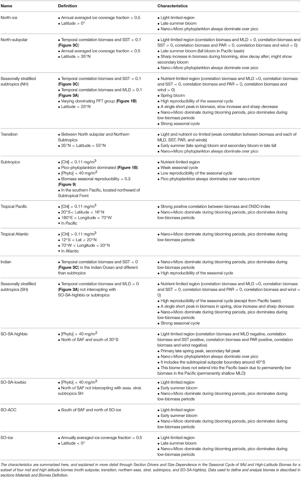
Table 1. Definition and characteristics of the biomes used in this paper, illustrated in Figure 1A.
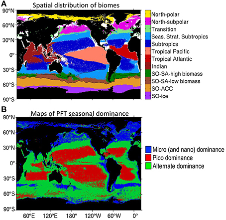
Figure 1. (A) Spatial distribution of the biomes defined in this paper. Biome definitions and properties are shown in Table 1. The subtropical Front and subAntarctic Front in the Southern Ocean are shown in black. (B) Maps of PFT seasonal dominance based on satellite biomass dataset. Three different regions arise depending on the dominating phytoplankton group (in absolute terms): (1) zones where pico- dominate over nano- and micro-phytoplankton throughout all year long (in red), (2) zones where nano- and micro- dominate over pico-phytoplankton throughout all year long (in blue), and (3) zones where both groups of phytoplankton dominate at some moment in the year (in green).
We use frontal structures to divide the Southern Ocean. The major fronts used here are the subtropical front (STF) and the subAntarctic front (SAF), as defined by Orsi et al. (1995) and downloaded from http://gcmd.nasa.gov/records/AADC_southern_ocean_fronts.html. We distinguish a region south of the seasonally stratified subtropical band but North of the SAF, which we divide further into a high biomass biome (in dark green in Figure 1A) and a low biomass biome (in brown in Figure 1A) and which we denote by SO-SA-highbio and SO-SA-lowbio, respectively (SA stands for SubAntarctic). Note that our SA region is similar to the Sallée et al. (2015) “Subantarctic” region (defined based on seasonality of Chl). South of the SAF we distinguish a subpolar region which mostly follows the meanders of the ACC which we denote as SO-ACC, as well as a region where the annual averaged ice fraction is larger than 0.5 denoted as SO-ice. Throughout the paper, the spatial averages over biomes take into account the unequal pixel and domain sizes.
Our resulting biome divisions are qualitatively similar to the ones by Oliver and Irwin (2008), which based their classification on a clustering algorithm without prior knowledge of the total number of regions. Our division is also qualitatively similar to the classification of Hardman-Mountford et al. (2008), which was solely based on multivariate statistics and classification techniques using the chlorophyll seasonal cycle.
Observational phytoplankton literature often looks at how much of the total biomass at a given location can be ascribed to one phytoplankton group vs. another. Our satellite dataset allows us to analyze PFT biomass—total biomass relationships by averaging our PFT biomass and total biomass data over each of our ecological biomes. In Figure 2A, we show that (a) for a given PFT group, data points representing different biomes fall on the same line and (b) biomes with a higher biomass are dominated by larger sizes. Pico- lines have a smaller slope than micro- lines, indicating that with increasing total biomass micro-phytoplankton are responsible for a larger fraction of the total biomass. This difference in slopes also means that large phytoplankton exhibit a larger range of biomass variability spatially than smaller phytoplankton. Oligotrophic regions with limited supply of nutrients and low total biomass, such as the subtropics, are dominated by pico-phytoplankton. Regions with plentiful nutrients and high biomass, such as the upwelling and high-latitude biomes, are dominated by large (nano- and micro-) phytoplankton, in agreement with in-situ and satellite data (see Introduction).
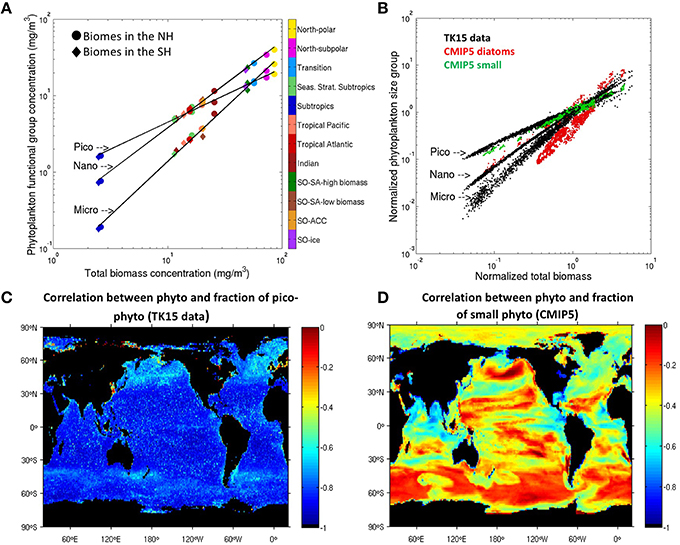
Figure 2. PFT biomass vs. total biomass in data and models. (A) Pico-, nano-, and micro- biomass vs. total phytoplankton biomass in the TK15 satellite dataset across biomes. Each color symbol represents the biomass spatially averaged in a given biome (as labeled), and temporally averaged over the complete monthly SeaWiFS time series. Black solid lines show the linear regression across the biomes for the three labeled PFT groups. (B) Each black dot shows a biome-averaged month from the complete SeaWiFS data series (1998–2010) in the TK15 dataset and for each PFT as labeled. All data points are normalized by dividing by the globally averaged PFT biomass. Colors show the same for the CMIP5 multi-model averaged diatom (green) and small phytoplankton biomass (red). Southern Ocean biomes are not shown in the multi-model average due to high dispersion but are shown in Figure S2. (C) Temporal monthly correlation between total phytoplankton biomass and fraction of pico-phytoplankton in TK15 data. (D) Temporal monthly correlation between total phytoplankton biomass and fraction of small phytoplankton in the CMIP5 multi-model average.
Additionally, points representing different months of the year also fall on the same PFT-specific lines (Figure 2B), demonstrating that this relationship also holds temporally across seasons. The proportion of small phytoplankton decreases during seasons with large biomass, therefore the time series of phytoplankton biomass and picophytoplankton percentage are inversely correlated everywhere, according to satellite biomass data (Figure 2C). High latitudes are dominated all year round by large phytoplankton (micro- and nano-) while low latitudes are dominated by picophytoplankton (Figure 1B). Mid-latitudes (such as the seasonally stratified subtropical biome) and upwelling regions have varying dominant size groups through the year (Figure 1B). Further exploration shows that during the blooming period in winter and spring the nano- (and micro-) dominate, while in summer (minimal total biomass) the pico-phytoplanktkon dominate, such that the area of pico-dominance (in red) shifts poleward seasonally in the warmer hemisphere and equatorward in the colder hemisphere.
We observe the same main patterns as Marañón (2015) North Atlantic data, such as increasing dominance of nanophytoplankton at large carbon biomass, followed by micro- and pico- (Figures S1A,B). Our results are surprisingly similar to their data if we take into account that the underlying KSM09 algorithm that is used to compute the TK15 biomass from backscattering is theoretical and doesn't use any empirical fitting. Agawin et al. (2000) compiled in-situ PFT data in units of chlorophyll from different regions representing all major oceans and interior seas under a wide range of nutrient conditions, and plotted pico- chlorophyll vs. the sum of nano- and microphytoplankton chlorophyll (Figure S1C). Our biomass data is qualitatively consistent with their results as well, as shown in Figure S1D. Again, as total phytoplankton Chl increases, the proportion of large sizes increases.
Assuming that this is a universal law of nature (as suggested by previous observational papers, e.g., Marañón, 2015) that extends also to the poorly sampled high latitudes, we would expect model PFTs to also follow these lines and expectations. The CMIP5 model diatom and small phytoplankton slopes are shown for comparison in colors in Figure 2B. Since the definition of diatoms (and equivalent approximate size) varies widely across models, we normalized each data point by the respective globally averaged PFT biomass in order to allow inter-model comparison and model-satellite data comparison (e.g., we divided the biomass of each PFT group in each pixel by the global spatially averaged biomass of each PFT). In general, the modeled average small phytoplankton behavior resembles the TK15 pico- behavior (green points) and the modeled average diatom behavior resembles the TK15 micro- behavior (red points), as expected (Figure 2B).
Significant variability with respect to the universal line (per PFT group) is seen, however, across CMIP5 models (Figure S2). Specifically, a significant deviation from the universal line is seen in the SO biomes in some CMIP5 models. Figure S2 shows that model diatom concentration is too high during winter months (i.e., at low total biomass concentrations) or conversely small phytoplankton concentration is too low in the SO in most models. This bias in models is also seen when temporally correlating phytoplankton biomass and small phytoplankton fraction. Figure 2D shows the multi-model averaged temporal correlation, which is negative but much weaker than in data. When looking at individual model correlations, we see that the models GFDL-ESM2G and GFDL-ESM2M exhibit a strongly negative temporal correlation (Figure S3), which agrees with our TK15 data and observational expectations. However, some models exhibit positive correlations in the Southern Ocean and high-latitude northern Pacific (CESM1-BGC and HadGEM2-ES), in the tropical areas (IPSL-CM5A-MR) or in different patches across the oceans (GISS-E2-H-CC, GISS-E2-R-CC). A positive correlation runs against expectations, since it implies a fractional increase of small phytoplankton (relative to larger phytoplankton) during high-biomass growing seasons.
The mixed layer depth (MLD) is one of the most important drivers for phytoplankton blooms as it controls the entrainment of nutrients, the availability of light in the euphotic layer, the rate of turbulent mixing, and the concentration of grazers, as described in the Introduction. While the trigger mechanism for blooms is still under debate, the scientific community agrees that the blooming ends due to nutrient depletion and increased grazing pressure.
Here, we show that biomass growth is consistent with a regime of light limitation at high latitudes (provided sufficient nutrients), such that a biomass bloom can be achieved by either decreasing the MLD or increasing the incoming phytosynthetically available radiation (PAR) (for example by melting ice). This is shown in Figure 3 for the satellite biomass data, where the light limited biomes show negative correlations between seasonal MLD and biomass (Figure 3A), and positive correlations between seasonal PAR and biomass (Figure 3B), such that phytoplankton growth coincides with an increase of light availability. These patterns were also observed by Wilson and Coles (2005) and Henson et al. (2009) when correlating seasonal MLD and Chl, and were reported by Barton et al. (2015) when correlating MLD and in in-situ phytoplankton time series. As stratification is mostly controlled by surface temperature, low sea surface temperatures (SST) usually correspond to deep MLD and high SST to shallow MLD. Then, correlations between SST and biomass are also useful indicators of light and nutrient regimes as seen in Figure 3C (see also Wilson and Coles, 2005; Barton et al., 2015).
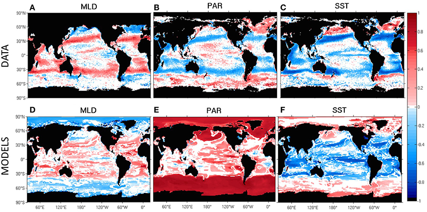
Figure 3. Temporal monthly correlation between the decimal logarithm of phytoplankton biomass and mixed layer depth (MLD), photosynthetically available radiation (PAR) and sea surface temperature (SST) during the SeaWiFS period (1998–2010) in TK15 data and observed fields (A–C) and in the CMIP5 multi-model mean (D–F). All the correlations are applied in each model separately with model-specific fields, and later averaged to obtain a multi-model average in which we weight each model equally. In (E), only four of the seven models were used (CESM1-BGC, GFDL-ESM2G, GFDL-ESM2M, and IPSL-CM5A-MR) due to output availability. All time series used were linearly detrended to avoid correlations associated with decadal or climate change trends. Non-significant correlations are shown as white.
At mid-latitudes in both hemispheres (30–45°), light is available throughout the year so the growth of biomass is usually nutrient limited, leading to correlations with MLD, SST, and PAR of the opposite sign as compared to more poleward latitudes (Figures 3A–C). In the transition regimes between the mid and high latitudes, there is a combination of the two mechanisms (light vs. nutrient limitation), where a bloom may have either subtropical or subpolar characteristics, and the correlations in Figure 3 are not significant (as also seen in Henson et al., 2009 using Chl instead of biomass in the North Atlantic). Low latitude oligotrophic gyres have less of a seasonal cycle, are permanently stratified, and have plenty of light all year round. Hence, the blooms occur during occasional nutrient entrainment events, coinciding with anomalous upwelling or wind mixing. This low seasonality translates into low correlations in Figures 3A–C.
The correlation patterns between wind speed and biomass (Figure S4) are similar to the correlation patterns between MLD and biomass, as stronger winds increase the influx of nutrients probably by deepening the MLD at mid latitudes (positive correlation) and decrease the availability of light necessary for phytoplankton growth at high latitudes (negative correlation). Similar patterns were also observed by Barton et al. (2015), with in-situ measurements of phytoplankton. Correlations between wind speed and satellite-derived Chl anomalies show qualitatively the same results (Kahru et al., 2010). Indeed, we have verified that wind speed and SST are negatively correlated in most of the oceans (as also shown in Kahru et al., 2010), while wind speed and MLD are positively correlated.
Similar correlations and regime changes are seen across CMIP5 models in Figures 3D–F, although models tend to show weaker correlations at mid and high latitudes compared to the data. Additionally, the positive correlation between biomass and PAR at high-latitudes is much more pronounced in models than in data and the strong negative correlation shown in data at mid-latitudes is not represented in models (compare Figure 3B with Figure 3E), suggesting that phytoplankton are more strongly limited by surface light PAR in models. The negative correlation between PAR and biomass observed in the northern seasonally stratified subtropical biome (discussed in more detail in Section Drivers and Size Dependence in the Seasonal Cycle of Mid and High-Latitude Biomes) is coincidental, as light peaks in summer and biomass peaks in winter (coinciding with maximum entrance of nutrients), with a lag of approximately 6 months (anti-correlation). However, models predict a later phytoplankton peak (in spring) compared to data (in winter) in this region. This bias in the modeled peak date removes in models the observed negative temporal correlation between PAR and biomass.
It is important to notice that correlations in the seasonal cycle between biomass and physical drivers do not prove strictly causality but rather qualitatively inform about seasonal regimes. We separately performed analogous correlations between anomalies (seasonal cycle removed) in biomass and anomalies in physical indices but these are very weak, suggesting that the processes are more complicated interannually (as shown for example in Lozier et al., 2011) and/or not instantaneous.
At high latitudes, the phytoplankton peak date propagates poleward, which is most evident in the North Atlantic (Figure 4A). In the NH light-limited high latitudes, the northward propagation is well explained by progressive shallowing of MLD as spring unfolds (Levy et al., 2005). Nutrients are already available during fall at high latitudes (Levy et al., 2005) but the blooming only happens in the spring after the MLD starts shallowing and light availability increases. In the subtropical gyres, nutrients become available around winter. This instantaneously initiates the blooming as light is already sufficient in this biome. Hence, the blooming peak date is in winter in the subtropics and gradually propagates poleward, with higher latitude peaks in spring and summer. The poleward progression of the Chl bloom has been widely studied, particularly for the North Atlantic (Dutkiewicz et al., 2001; Siegel et al., 2002; Levy et al., 2005; Henson et al., 2009; Racault et al., 2012). We find phytoplankton biomass to peak at similar times as Chl (compare Figures 4A,B).
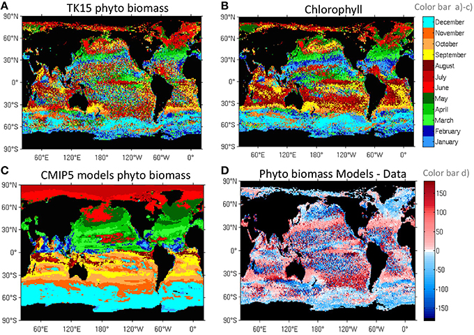
Figure 4. Blooming Peak date. Peak date in the climatological seasonal cycle for (A) TK15 8-day phytoplankton, (B) 8-day chlorophyll, (C) monthly CMIP5 multi-model averaged phytoplankton (top color bar), and (D) difference between CMIP5 models (C) and data (A) (in days), where red means data leads and blue means models lead (bottom color bar).
The same general blooming peak progression applies to the rest of the oceans as already shown for Chl by Racault et al. (2012). However, the data shows clear asymmetries between the North Atlantic and Pacific basins. In the North Pacific, the peak occurs later (Figure 4A) and shows larger interannual variability (see lower interannual variation in the peaking date in the North Atlantic in Figure S5A), as also seen by Racault et al. (2012) and Cole et al. (2015).
The patchy and somewhat banded blooming structure in the Southern Ocean (Figure 4A) is related to frontal structures. The blooming peak occurs during early summer (December) in the SO-ACC biome (between the Subantarctic Front and the sea ice biome), and later in summer (January-February) in the southernmost sea-ice regime.
The multi-model averaged total phytoplankton biomass peaks later than the satellite-derived phytoplankton at mid latitudes (Figures 4C,D), for example in the northern seasonally stratified subtropical biome (Figure 1A). The reason for this discrepancy can be attributed to a delayed deepening of the MLD in models as seen in Figure S5B. On the contrary, the modeled biomass peaks earlier at high latitudes (north and south of 45°N and 45°S), for example in the subpolar biome. Differences in high latitudes have not yet been attributed to discrepancies in a specific forcing factor. Models show diatoms blooming earlier than small phytoplankton in most regions (not shown), while the data show similar peaking times for all sizes, which is discussed in more detail in Section Drivers and Size Dependence in the Seasonal Cycle of Mid and High-Latitude Biomes.
We focus here on four biomes that exhibit clear seasonality and are located at mid and high latitudes. These are the north subpolar, transition, northern seasonally stratified subtropics, and Southern Ocean Subantarctic high biomass (SO-SA-highbio) biomes and are described in Section Biomes Definition, Table 1, and illustrated in Figure 1A.
We show the seasonal evolution of a series of common bottom-up drivers (MLD, PAR, SST, winds, nitrate) for each biome in Figures 5A, 6A, 8A and Figure S8A. As seen in these figures and discussed in detail in Section Drivers of Seasonality in Phytoplankton Carbon Biomass, the MLD achieves its maximum during the hemispheric late winter at mid and high latitudes. The MLD gradually decreases in the spring and remains shallow until it rapidly deepens during the following winter. Wind speed usually peaks in the middle of the winter and is at its minimum in the middle of the summer. The supply of nutrients to the euphotic layer increases a few days after the deepening of MLD. Light (PAR) peaks in late spring (June in the NH) and SST peaks later in the summer. Top-down factors, such as grazing, will also control the intensity, shape, and timing of the bloom (e.g., Siegel et al., 2002; Behrenfeld, 2010) but are not illustrated in this study.
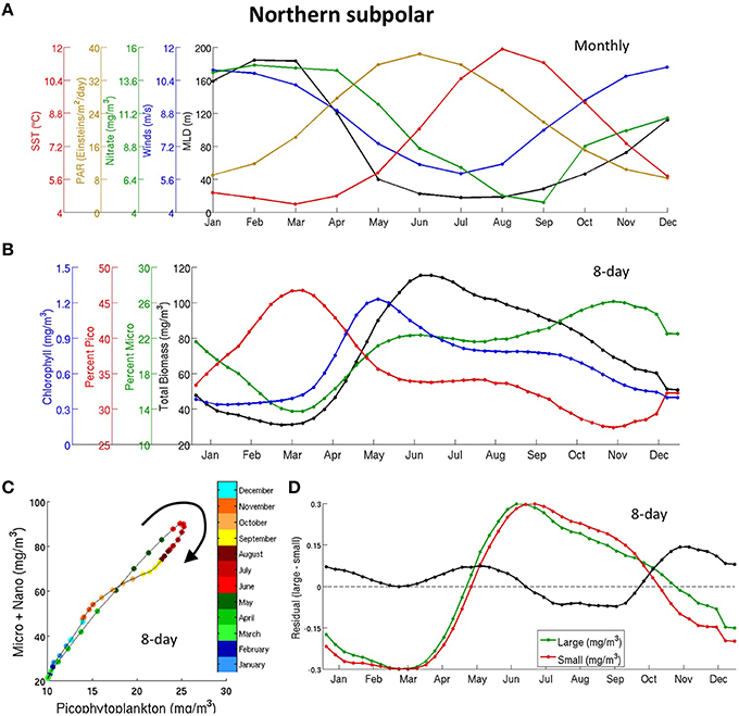
Figure 5. Seasonal cycle of bottom-up drivers (A) and different PFT (B) in the northern subpolar biome, (C) seasonal cycle of micro- and nano- phytoplankton (summed) plotted against pico-phytoplankton, (D) Normalized (0–1, labels not shown) seasonal cycle for micro- and nano- phytoplankton together (green), pico-phytoplankton (red), and residual (micro- plus nano- minus pico- in black, y-labels apply only to the residual). The seasonal cycles are normalized by subtracting the minimum value and dividing by the maximum value in (D). The 8-day data in (B–D) is smoothed with a top-hat filter of 31 days.
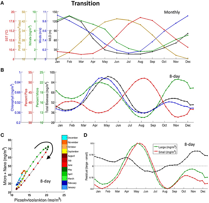
Figure 6. Same as in Figure 5 for the transition biome in the Northern Hemisphere.
In the Atlantic and the Pacific north of 30°N the following three regions with high phytoplankton seasonality clearly emerge: (a) the subpolar regime N of about 50°N, with a single (June-July) light-limited biomass peak, (b) a transitional regime roughly between 45 and 50°N characterized by light-nutrient co-limited phytoplankton with two annual biomass peaks, (c) the seasonally varying northern subtropical regime from 30 to ~45°N, with nitrogen limited phytoplankton characterized by a single annual peak in winter or early spring.
In line with Sverdrup's critical depth theory, deep wintertime mixing in the Northern Subpolar biome ensures light limitation and very little production and zooplankton population in winter. Gradual increase in PAR and shallowing of MLD increases the light availability in the mixed layer in the spring. The release of light limitation, coupled with a slow recovery of zooplankton (or large zooplankton that do not respond fast enough to growing phytoplankton populations) allows a late spring or early summer phytoplankton bloom of phytoplankton (Figures 5A,B). Phytoplankton slowly decline throughout the summer and fall as they gradually deplete nutrients and are eaten by grazers and achieve minimal levels during the following winter. A closer inspection of the results shows significant differences between the Atlantic and the Pacific basins. In the North Atlantic, we recognize an early summer bloom, which coincides with an increase in surface light PAR, and a weaker late fall bloom, which coincides with a decrease in light and increase in nitrate (Figures S6A,B). On the other hand, the North Pacific shows a single flat bloom that lasts from late spring to late summer (Figure S7B). We note also that biomass-physical driver correlations in Figure 3 are generally weaker in the subpolar North Pacific, in agreement with a higher interannual variability in the peak date (Figure S5A). Possible explanations for differences across these basins are detailed in the Discussion. CMIP5 models show that phytoplankton also peak around late spring in the north subpolar biome, although slightly earlier than observed (Figure 4D and Figure S9).
The fraction of observed large PFTs increases during the spring bloom as total biomass increases (Figure 5B), as expected from in-situ observations and discussed in Section General Patterns in Phytoplankton Size Classes and Figure 2B. The large species (micro and nano) grow slightly earlier than pico-phytoplankton in the spring bloom (Figures 5C,D), which suggests that large sizes are more responsive to changes in nutrients and light or less responsive to top-down control. However, a closer look across basins reveals that the distinctive succession of species during the spring bloom in the biome average is driven by phytoplankton in the Pacific basin.
The seasonal succession of species in models is similar to observations (on average) during the spring bloom, as most CMIP5 modeled diatoms bloom earlier by about a month (Figure S9) than small phytoplankton, with the exception of the model CESM1-BGC. However, the seasonal cycles of diatoms and small phytoplankton are more clearly differentiated—uncoupled—in models compared to data. This becomes apparent in comparing the large-small phytoplankton phase plots in SeaWiFS and the individual CMIP5 models (see Figure S9).
Although Chl and carbon biomass have a similar seasonal cycle and are strongly coupled, Chl starts increasing and peaks earlier (by about a month) than carbon phytoplankton biomass during the spring bloom. Behrenfeld et al. (2005) finds similar seasonal differences between Chl and a satellite derived carbon biomass (different from our product) over the equivalent biome and interprets them as an initial cell pigmentation (Chl) followed by increase in growth and biomass.
The growth of phytoplankton in the transition zone is limited by both light as in the subpolar biome and nutrients as in the northern seas. strat. subtropics (Figures 6A,B), in agreement with findings by Henson et al. (2009). This biome is located in the transition between positive MLD-biomass correlation (nutrient-limited) and negative MLD-biomass correlation (light-limited)—Figure 3A. Biomass is at its minimum when either MLD or PAR are at their minimum (Figures 6A,B). This suggests a clear alternation of light and nutrient limited conditions: light limitation in winter, growth in spring, nutrient limitation in the summer, and growth in the fall. The bimodal peak structure was previously noted in Chl satellite data by Sapiano et al. (2012). Figure 7 shows the geographical shift from one single winter bloom (northern seas. strat. sub. biome) to two blooms (transition biome) across a transect in the North Atlantic at 40°W.
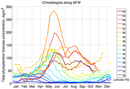
Figure 7. Averaged seasonal cycle (climatology) of TK15 phytoplankton concentration in a transect across the North Atlantic at 40°W, at different northern hemisphere latitudes as labeled.
The largest (primary) bloom occurs during spring (May), coincident with an increase in light availability and plentiful nutrients that trigger a rapid response in large PFTs growth and a slightly slower response in small PFTs (Figures 6C,D) as in the subpolar biome. All the PFTs peak at similar times. Biomass declines as summer progresses and MLD shallows, which limits nutrients and increases the pressure from grazers (Figure 6B). The secondary bloom occurs during the fall and is dominated by large phytoplankton (Figure 6B). At this time, there is still enough light to facilitate phytoplankton growth and MLD begins to deepen, bringing more nutrients back into the region. As in the subpolar biome, Chl grows slightly earlier than total phytoplankton biomass (Figure 6B).
The seasonal cycles of diatoms and small phytoplankton are more strongly uncoupled in CMIP5 models than in data (Figure S9) as already seen in the subpolar biome. The seasonal succession is similar to the one in the subpolar biome, where diatoms grow earlier than small phytoplankton. Finally, CMIP5 models fail to capture the secondary peak.
The growth of phytoplankton is essentially limited by nutrients in this biome (strong bands of positive MLD-biomass correlation in Figure 3A and negative SST-biomass correlation in Figure 3C); therefore, phytoplankton peak in late winter (February and March) when nutrients increase following a deepening of the MLD (Figures 8A,B). Conversely, MLD is at its minimum in the late summer months, when biomass is at its minimum (Figures 8A,B). These are regions with a single annual biomass peak (as shown in Figure 7B in Sapiano et al., 2012). Chl follows carbon very tightly in this biome (Figure 8B), more so than in the subpolar and transition biomes. We find that phytoplankton bloom later in most CMIP5 models than in observations (Figure 4D and Figure S9) and we hypothesize that this is due to a consistently later deepening of the MLD in models, as indicated by Figure S5B.
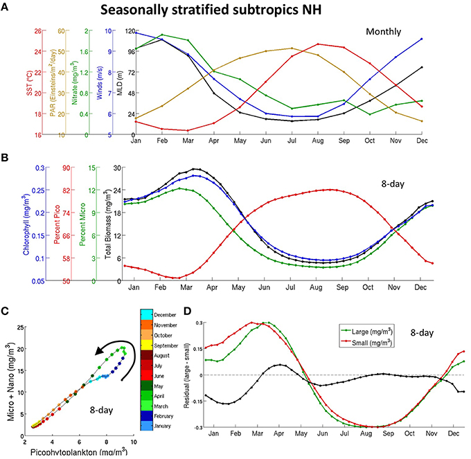
Figure 8. Same as in Figure 5 for the northern subtropical biome.
In this biome, the Atlantic and Pacific basins show similar seasonal responses. The Atlantic section of the seasonally-stratified subtropics coincides with the “mid-latitude” biome defined in Levy et al. (2005) and described as a nutrient-limited region, in accordance with our results. The Pacific part of this biome includes the Transition Zone Chlorophyll Front (TZCF) identified as a maximum in the meridional gradient of Chl as well as the 18°C isotherm and shown to migrate from 30–35°N in winter to 40–45°N in summer (Bograd et al., 2004).
The northern seasonally stratified subtropics are relatively dominated by nano- (and micro)-phytoplankton during the bloom months, and by pico-phytoplankton during the low-biomass summer months (Figure 8B), as expected from in-situ observations and shown in Figure 2B. However, pico-phytoplankton increase earlier than large phytoplankton during the bloom (Figures 8C,D). Phase plots showing diatoms vs. small phytoplankton throughout the year were analyzed across CMIP5 models (Figure S9). The seasonal cycles of diatoms and small phytoplankton are more uncoupled in 6 out of 7 models compared to observations (compare first panel in Figure S9 with the rest of panels), as was also the case in the previous biomes. Two of the models (GISS-E2-R-CC and IPSL-CM5A-MR) show that small phytoplankton grow earlier than diatoms (anti-clock wise phase plots) as observed, while four models show that diatoms grow earlier than small phytoplankton (clock-wise phase plots).
The phytoplankton seasonality of SO-SA-highbio biome is very similar to the one in the northern subpolar biome (once corrected from the 6-month phase difference between the SH and NH), which suggests that the growth of phytoplankton is explained by similar mechanisms in the northern subpolar biome and in the SO-SA-highbio biome. Indeed, strongly positive SST-biomass correlations and strongly negative MLD-biomass correlations in SO-SA-highbio point to a strong light limitation in this region (Figures 3A,C) as in the northern subpolar biome; we note that these correlations are either insignificant or of opposite sign in the rest of the SO. Hence, blooming occurs in the spring (November) as the MLD shallows and light both at the surface and in the mixed layer average increases (Figure 4A, Figures S8A,B). Biomass blooming is preceded by an increase in Chl (Figure S8B) as in the northern subpolar biome (Figure 5B). We find that phytoplankton biomass decays slowly after the peak and blooms again in late fall (April-May, Figure S8B).
This biome stands out as a region with dominance of nano- and micro- over pico- throughout the year (blue in Figure 1B), as expected in regions with high biomass (Figure 2A). Note that the dominance of pico and nano+micro alternates throughout the year in the rest of SO biomes probably due to strong iron limitation, contrary to similar biomes in the NH. As in the northern transitional and subpolar biomes, the fraction of observed large PFTs increases during the spring bloom and even more during the secondary bloom (Figure S8B). The CMIP5 models misrepresent the SO-SA-highbio biome with two blooms and less Fe-limited than the rest of the SO. Models show a single peak (Figure S9D), and fewer phenological differences across basins (e.g., compare Figures 4A,C) compared to observations. Finally, the seasonal cycles of diatoms and small phytoplankton are more clearly differentiated—uncoupled—in models compared to data in the SO-SA-highbio, as in the other discussed biomes, although most models agree in that the growth of diatoms occurs earlier than small phytoplankton.
The year to year reproducibility of the mean seasonal cycle is studied following the description of Thomalla et al. (2011) and described in Section Phenological Indices. The low latitudes show a low reproducibility of the seasonal cycle because (a) the seasonal cycle is nearly flat, and (b) phytoplankton growth depends on occasional/episodic nutrient supply events not related to the main seasonal cycle (Figure 9). At mid and high latitudes, the seasonal cycle is usually more reproducible. In this case, a low correlation indicates a high interannual (rather than seasonal) variability in blooming magnitude or peaking date, or the presence of more complicated patterns such as multiple blooming peaks, which might vary their relative intensity and timing interannually, and hence reduce the reproducibility (Figure 9).
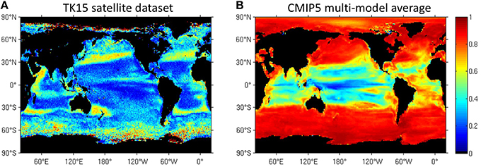
Figure 9. Reproducibility of the seasonal cycle (Monthly temporal correlation between the complete SeaWiFS time series phytoplankton linearly detrended in log10 space and the repeated climatology) in (A) data and (B) models.
The seasonal cycle is highly reproducible year to year in two subtropical bands around 35–40°N and 35–40°S (Figure 9A) that approximately coincide with the seas. strat. subtropical biomes (illustrated in Figure 1A). These bands match the patterns observed by Yoder and Kennelly (2003), Doney et al. (2003), Vantrepotte and Melin (2009), Sapiano et al. (2012), and Thomas et al. (2012). When the seasonal cycle contributes strongly to the total variance, the seasonal cycle tends to be stable from year to year; this translates into low interannual variability (not shown). The biomes located poleward of the high-seasonality bands show less reproducibility of the seasonal cycle (Figure 9A), or conversely more interannual variability. In the North Atlantic, the variability in the transition region is associated with NAO phases (Henson et al., 2009).
The reproducibility of the seasonal cycle is much higher in CMIP5 models (Figure 9B) compared to data (Figure 9A), probably due to a simplification of physical and biogeochemical drivers of phytoplankton growth coupled with an underestimation of natural variability in physical drivers. The failure to capture secondary blooms in models also facilitates a higher reproducibility of the seasonal cycle. Henson et al. (2009) observed the same model-to-data bias when comparing the seasonality of satellite-derived Chl to an older version of the GFDL model.
In Figure 10 we characterize the strength of the annual peak as the linear difference in logarithmic space between the maximum and the minimum biomass in the seasonal cycle (related to the percent increase). The mid latitude seasonally stratified subtropics (Figure 1A) stand out as one of the regions with the highest strength in the seasonal cycle (Figure 10A), which coincides with areas with high reproducibility in Figure 9A and areas with a single bloom in Sapiano et al. (2012). In the North Atlantic, Ueyama and Monger (2005) show a zone with high relative bloom magnitude (defined as the bloom magnitude divided by the non-bloom-period magnitude) that coincides with our observed North Atlantic band. The strength of the seasonal cycle increases gradually poleward in CMIP5 models (Figure 10D), which differs from the more noticeable bands just described in observations (Figure 10A).
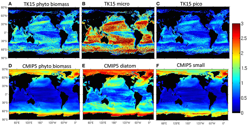
Figure 10. Seasonality strength. Strength of the seasonal cycle [LOG10(MAX biomass)-LOG10(MIN biomass)] across data (A–C) and CMIP5 multi-model average (D–F) as labeled.
Everywhere in the ocean, the blooming is stronger—larger logarithmic increase in biomass from the minimum to the maximum annual biomass—for large compared to small sizes (compare Figures 10B,C). This can be explained by the rapid response of diatoms to sporadic changes in growth factors such as winter storms and wind-driven pulses of nutrients (Fogg, 1991), but also to other factors explained in the Introduction. On the other hand, small phytoplankton are more favored by constant background conditions, which translates into a less strong seasonal cycle in Figure 10C for pico-phytoplankton. Most CMIP5 models capture also a stronger seasonal cycle in diatoms (Figure 10E) compared to small phytoplankton (Figure 10F).
An emergent characteristic that separates light-limited from nutrient-limited regions is the “skewness” of the seasonal cycle. We illustrate this novel phenological indicator in Figure 11. Phytoplankton in light-limited biomes (especially clear in the northern subpolar and SO-SA-highbio) start to bloom suddenly and decay to minimum values slowly (blue in Figure 11A), while in nutrient-limited biomes (e.g., northern seas. strat. subtropics) they decay suddenly (red in Figure 11A). This transition in seasonal skewness is also seen around 45°N in a 40°W transect across the North Atlantic (Figure 7). The skewness of the seasonal cycle in CMIP5 models is similar to observations, although the transition from the subpolar biome to the northern seas. strat. subtropical biome (clearly seen in observations) is less sharp in models and positioned more equatorward.
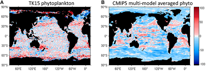
Figure 11. The skewness of the seasonal cycle around the peak, calculated as the difference (in days) between the time needed to increase the biomass from a 40% threshold to the peak biomass and the time needed to decrease the biomass from its peak value back to the same threshold, in (A) TK15 and (B) CMIP5 multi-model average phytoplankton. Red areas indicate a slow increase and a sharp decrease in biomass (e.g., see the northern subtropics), while blue areas indicate a sharp increase and slow decrease (e.g., see the northern subpolar biome). The maps were spatially smoothed with a Gaussian filter with a standard deviation of 2°.
Much previous research has been done looking at the seasonality of chlorophyll. Here instead we focus on the seasonality in total biomass and biomass size groups over the 1998–2010 SeaWiFS period.
Biomes and seasons with high phytoplankton biomass show an increase in the fraction of large PFTs, in agreement with in-situ and laboratory studies and current understanding of ecosystem dynamics (Figure 2, Figures S1–S3). This results in stronger blooms associated with larger species (Figure 10B). Areas with large seasonal variability in physical drivers exhibit high seasonality in phytoplankton (high latitudes, Figure 9) and are dominated by large phytoplankton, while areas with low seasonal variability in drivers (low latitudes) exhibit low seasonality in phytoplankton and small-phytoplankton persistence. The modeled CMIP5 diatoms behave similarly to the observed micro- and nano-phytoplankton, while the modeled small phytoplankton behave similarly to the observed pico-phytoplankton. This resemblance between models and data is remarkable given the differences in definition between satellite PFTs used here and the groups defined by the different CMIP5 groups. An important deviation from observations that needs further study was found in a subgroup of models, where an increased fraction of small phytoplankton was found during bloom conditions in some regions.
At high latitudes, light is the main limiting factor and the initiation of the bloom is believed to be rapid once the light limitation on growth is relieved in the spring by shallowing MLDs. Phytoplankton biomass decays slowly after the peak, as shown by the novel skewness indicator in Figure 11A. The slow phytoplankton decay after the peak could be due to the persistence of nutrients that keep the biomass high until light becomes limiting in late fall. The slow decay could also be due to increased dilution of grazers (decreased zooplankton pressure) when MLD starts deepening again after the summer. There are, however, differences between basins. While the North Atlantic shows a main spring bloom and a weak late fall bloom, the North Pacific shows a single flat bloom that lasts from late spring to late summer (Figures S7A,B). In the North Atlantic, the initiation of the chlorophyll spring bloom has been associated to an increase in insolation (Racault et al., 2012) or to reduced turbulent mixing in the surface (Cole et al., 2015). These studies agree that in contrast bloom initiation cannot be clearly associated to a singular driver in the North Pacific. The North Pacific has overall lower wintertime MLDs because of its fresher surface waters and more stratified watercolumn; it also has less seasonality in MLDs compared to the North Atlantic. This suggest that the North Pacific suffers less from light limitation than the North Atlantic. Another possible explanation for the different phytoplankton behavior in the North Pacific would be that the persistently shallower MLD in the North Pacific (particularly in the eastern side of the basin) allows primary production and the grazer population to be sustained through winter, such that the spring bloom can be reduced by grazers as soon as it starts (as summarized in Cole et al., 2015). Iron limitation also plays a role in the North Pacific HNLC (high nutrient low chlorophyll) region, such that the bloom only starts when sufficient iron is available. The larger interannual variability in the North Pacific bloom timing compared to the Atlantic (as seen from Figure S5A) could be linked to strong variability in climate indices such as ENSO or Pacific Decadal Oscillation as summarized by Cole et al. (2015).
The fraction of large PFTs increases during the spring biomass peak and increases even more during the secondary fall peak at high latitudes (as shown in Figures 5B, 6B and Figures S6–S8). Thus, small PFTs show a less prominent secondary peak with respect to the spring peak when compared to large PFTs. While we do not have grazer observations, the bottom-up controls and PFT biomass patterns we see agree with the theoretical picture proposed by Sommer (1996) in the North Atlantic. According to Sommer (1996), bottom-up controls (increased light in our case) trigger the Atlantic early summer bloom after a winter period with no phytoplankton or grazers. This spring bloom is followed by a rise in zooplankton that contributes to the decline of phytoplankton. Later on in subsequent blooms, selective grazing on small phytoplankton leads to a greater fractional dominance of larger species when compared to the primary bloom. This means that selective grazing does not affect the spring bloom (which is thought to be controlled mainly by bottom-up drivers) but prevents small phytoplankton to bloom during the fall in the North Atlantic. Hence, the growth of large and small sizes is simultaneous in the North Atlantic subpolar biome during the spring bloom (Figures S6C,D). A selectively stronger grazing on small phytoplankton active from the start of the blooming period might explain why pico-phytoplankton increase later and decline earlier than micro-phytoplankton in the Pacific biome (Figures S7C,D).
In the Southern Ocean, the SO-SA-highbio includes the subtropical-subpolar boundary (shown in Figure 1A) between the warm and salty thermocline waters of the subtropical gyres and the colder, fresher subpolar regime. This frontal structure, located around 40–45°S in the Atlantic, Indian and W Pacific, corresponds roughly to the zero surface wind stress curl, and thus marks the transition between the nitrogen-limited downwelling subtropics and the iron and light co-limited upwelling subpolar gyre. Previous modeling work has suggested that lateral Ekman advection bringing high nitrate from the subpolar regions northward acts to concentrate maximum ocean primary production there (Marinov et al., 2013) as seen across the CMIP5 models (Cabré et al., 2015). Sallée et al. (2015) suggested that high productivity is due to relatively high Fe utilization downstream of major western boundary currents flowing on the Northern edge of the ACC, as this region contains the largest number of continental sources of Fe in the Southern Ocean (e.g., tip of South America, Falkland Islands, South Africa, Tasmania, New Zealand). Sallée et al. (2015) argued that the lack of Fe limitation allows for the presence of a bottom-up controlled spring bloom (associated with rapid light improvement caused by a reduction in surface-layer turbulence) and a top-down controlled fall bloom (controlled by a decreased prey-grazer encounter when the mixed layer de-stratifies) in the Subantarctic zone, consistent with our findings (Figure S8). South of the Subantarctic Front, the macro-nutrient rich, iron and light co-limited ACC regime (SO-ACC) follows the meanders of the ACC and is an HNLC regime. The seasonal cycle of this regime is characterized by a single large annual biomass peak in models but is incompletely represented in data because of lack of satellite coverage.
At lower latitudes, nutrients are limiting and the bloom is associated with the winter entrainment of nutrients when MLD is deepest. The bloom decays suddenly once nutrients are exhausted and grazing increases (red in Figure 11A). Hence, the skewness of the seasonal cycle emerges as a useful index to separate light-limited (sharp increase and slow decay) from nutrient-limited regimes (slow increase and sharp decay). In our satellite data the northern seas. strat. subtropics biome—limited by nutrients—broadly stands out as a highly seasonally variable region (Figure 9A); this high variability is primarily driven by changes in wind patterns. During the winter and early spring, stronger vertical mixing (more upward Ekman pumping, deeper MLDs) enhances the supply of nutrient while PAR is relatively adequate; these conditions enhance phytoplankton growth and push the Chl fronts equatorward. Conversely, an increase in surface heat flux into the ocean results in stronger stratification during the summer (May to August), which reduces vertical nutrient flux and pushes the fronts poleward. In the northern seasonally-stratified subtropical biome the pico- bloom earlier than micro-, suggesting a different combination of bottom-up and top-down controls compared to the more northern biomes (Figure 8).
The reproducibility of the seasonal cycle year by year is much higher in models, such that blooming periods are more predictable compared to satellite data (Figure 9). This is probably due to over-simplification of processes and a lower response to various climate oscillations, as well as a relatively coarse (nominally 1°) resolution, which does not allow a proper representation of coastal processes and some frontal dynamics in models. The simplification in models can also be observed in global patterns, as all the models display a smooth latitudinal propagation of the studied phytoplankton phenological indices, while the satellite-derived data display pronounced patterns such as the mid-latitude bands around 40°S and 40°N (e.g., Figures 9, 10). Diatoms start growing and peak earlier than small phytoplankton at all latitudes (not just in subpolar and transition biomes) in most CMIP5 models. Moreover, the temporal succession of species is clearer in the models compared to satellite biomass observations: the seasonal cycles of large and small phytoplankton are less coupled—i.e., they develop more independently with respect to each other—in models (compare SeaWiFS panel and individual models in Figure S9). This difference might be partly due to the definition of diatoms across CMIP5 models, which does not precisely correspond to the group nano+micro in our observational dataset. The degree of this PFT uncoupling varies also across models, and little work has so far explored this topic. Hashioka et al. (2013) studied succession in a subgroup of CMIP5 models and concluded that the succession of modeled PFT species during the bloom depends strongly on the choice of parameters for the modeled bottom-up and top-down equations such that no clear and unique mechanism arises across all the models.
Some of the problems in models might be fixed by modeling the distribution of traits (e.g., nutrient affinity) instead of phytoplankton functional types. Emerging trade-based modeling frameworks include selecting traits randomly from high dimensional trait space (Follows et al., 2007), game theory approaches (Litchman et al., 2009) and allowing flexible or optimal allocation strategies of cell internal resources in response to changes in the environment (e.g., Klausmeier et al., 2004; Smith et al., 2011; Clark et al., 2013; Pahlow and Oschlies, 2013; Smith et al., 2015). Depending on the spatial or temporal evolution of the environment, an organism might have to choose to invest in competitive abilities vs. defense against predation (Yoshida et al., 2003), or in nutrient vs. light uptake to optimize physiological acclimation (Smith et al., 2015). Investment into light harvesting vs. nutrient uptake vs. predation defense varies in the real ocean seasonally. A flexible modeling approach is encouraging as it might fix some of the issues we found in CMIP5 models—where traits are currently fixed rather than flexible (e.g., the half saturation coefficients for nutrient uptake are constants). Such CMIP5 model issues include the absence of secondary blooms in the mid-latitude transition biomes and the unrealistic dominance of small phytoplankton during blooms in the light and Fe co-limited Southern Ocean and North Pacific HNLC regions in some models (Figure S3). Models tend to not represent well observed seasonal indices in the HNLC regions. We suggest that CMIP5 models do not represent HNLCs well due to a simplification of processes, such as an incomplete or inflexible seasonal switching between top down and bottom up controls, or between light and Fe limitation of phytoplankton.
The discrepancy between models and data is partially a consequence of oversimplified biological bottom-up drivers and zooplankton grazing in models, but also a consequence of possible biases in the satellite-derived data. The algorithm to retrieve the underlying PSDs is purely theoretical (does not have an empirical constraint), and the biomass retrieval is subject to a series of assumptions that can accumulate to a large quantifiable and non-quantifiable uncertainty budget (Kostadinov et al., 2015). However, an empirical correction to the TK15 data is planned to address the apparent underestimates in the gyres and some overestimates in eutrophic areas (observed in Kostadinov et al., 2015). Thus, we caution against interpreting satellite data—model differences as only due to model error, i.e., satellite data should not be treated as the absolute truth. Innovative ocean color products such as the PFT-partitioned carbon biomass used here are very hard to validate due to the extreme lack of corresponding in-situ data. In spite of these limitations, we have previously shown that our satellite product exhibits a reasonable fidelity and compares favorably with other approaches, especially in terms of fractional biomass (Kostadinov et al., 2015). An ongoing study compares phytoplankton phenology across 10 satellite-based algorithms, including our current algorithm (Kostadinov et al., in prep.). Satellite ocean color observations are an invaluable tool for deeper understanding of the global marine ecosystem, since they provide a synoptic view of phytoplankton biomass distribution at a spatial resolution much higher than the current generation of Earth System models. Future hyperspectral missions such as the planned NASA PACE mission will increase the number of degrees of freedom available for ocean color observations and should enable simultaneous and improved retrieval of various phytoplankton groups at the global scale. Continuous improvement of optical algorithms, as well as intensified collection of in-situ organic carbon pools for algorithm validation are needed to help clarify the coupling between seasonal cycles of different PFTs and confirm the emerging satellite patterns. Future studies should also focus on the difference between chlorophyll and biomass succession, as these could improve our understanding of physiological responses such as photoacclimation, a topic we have not addressed here.
AC and IM conceived the manuscript. AC led manuscript preparation and writing. DS prepared the final figures. TK provided the TK15 dataset used in the manuscript. All the authors contributed to the editing of the manuscript.
The authors declare that the research was conducted in the absence of any commercial or financial relationships that could be construed as a potential conflict of interest.
AC, IM, and TK acknowledge support by NASA ROSES Ocean Biology and Biogeochemistry (OBB) grant NNX13AC92G and by a University of Pennsylvania (UPENN) Research Foundation grant. DS acknowledges summer support from a UPENN CURF fellowship and a UPENN Geosciences fund summer grant. We also acknowledge Hubert Loisel for providing his algorithm code and H. Loisel and David Dessailly for support. We acknowledge the World Climate Research Programme's Working Group on Coupled Modeling, which is responsible for CMIP, and we thank the climate modeling groups (listed in Table S1 of this paper) for producing and making available their model output. For CMIP the U.S. Department of Energy's Program for Climate Model Diagnosis and Intercomparison provides coordinating support and led development of software infrastructure in partnership with the Global Organization for Earth System Science Portals. We thank UPENN student Danica Fine for technical help in the initial part of the project.
The Supplementary Material for this article can be found online at: http://journal.frontiersin.org/article/10.3389/fmars.2016.00039
Agawin, N. S. R., Duarte, C. M., and Agusti, S. (2000). Nutrient and temperature control of the contribution of picoplankton to phytoplankton biomass and production. Limnol. Oceanogr. 45, 591–600. doi: 10.4319/lo.2000.45.3.0591
Alvain, S., Loisel, H., and Dessailly, D. (2012). Theoretical analysis of ocean color radiances anomalies and implications for phytoplankton groups detection in case 1 waters. Opt. Express 20, 1070–1083. doi: 10.1364/OE.20.001070
Alvain, S., Moulin, C., Dandonneau, Y., and Breon, F. M. (2005). Remote sensing of phytoplankton groups in case 1 waters from global SeaWiFS imagery. Deep. Res. I Oceanogr. Res. Pap. 52, 1989–2004. doi: 10.1016/j.dsr.2005.06.015
Alvain, S., Moulin, C., Dandonneau, Y., and Loisel, H. (2008). Seasonal distribution and succession of dominant phytoplankton groups in the global ocean: a satellite view. Glob. Biogeochem. Cycles 22:GB3001. doi: 10.1029/2007gb003154
Atlas, R., Hoffman, R. N., Ardizzone, J., Leidner, S. M., Jusem, J. C., Smith, D. K., et al. (2011). A cross-calibrated multiplatform ocean surface wind velocity product for meteorological and oceanographic applications. Bull. Am. Meteorol. Soc. 92, 157. doi: 10.1175/2010BAMS2946.1
Barber, R. T. (1988). “Ocean basin ecosystems,” in Concepts of Ecosystem Ecology: A Comparative View, Vol. 67, eds L. R. Pomeroy and J. J. Alberts (Berlin: Springer), 171–193.
Barton, A. D., Lozier, M. S., and Williams, R. G. (2015). Physical controls of variability in North Atlantic phytoplankton communities. Limnol. Oceanogr. 60, 181–197. doi: 10.1002/lno.10011
Behrenfeld, M. J. (2010). Abandoning Sverdrup's Critical Depth Hypothesis on phytoplankton blooms. Ecology 91, 977–989. doi: 10.1890/09-1207.1
Behrenfeld, M. J. (2014). Climate-mediated dance of the plankton. Nat. Clim. Chang. 4, 880–887. doi: 10.1038/nclimate2349
Behrenfeld, M. J., Boss, E., Siegel, D. A., and Shea, D. M. (2005). Carbon-based ocean productivity and phytoplankton physiology from space. Global Biogeochem. Cycles 19:GB1006. doi: 10.1029/2004GB002299
Bograd, S. J., Foley, D. G., Schwing, F. B., Wilson, C., Laurs, R. M., Polovina, J. J., et al. (2004). On the seasonal and interannual migrations of the transition zone chlorophyll front. Geophys. Res. Lett. 31:L17204. doi: 10.1029/2004gl020637
Brewin, R. J. W., Sathyendranath, S., Hirata, T., Lavender, S. J., Barciela, R. M., and Hardman-Mountford, N. J. (2010). A three-component model of phytoplankton size class for the Atlantic Ocean. Ecol. Modell. 221, 1472–1483. doi: 10.1016/j.ecolmodel.2010.02.014
Bricaud, A., Ciotti, A. M., and Gentili, B. (2012). Spatial-temporal variations in phytoplankton size and colored detrital matter absorption at global and regional scales, as derived from twelve years of SeaWiFS data (1998-2009). Global Biogeochem. Cycles 26:GB1010. doi: 10.1029/2010GB003952
Brody, S. R., and Lozier, M. S. (2014). Changes in dominant mixing length scales as a driver of subpolar phytoplankton bloom initiation in the North Atlantic. Geophys. Res. Lett. 41, 3197–3203. doi: 10.1002/2014GL059707
Cabré, A., Marinov, I., and Leung, S. (2015). Consistent global responses of marine ecosystems to future climate change across the IPCC AR5 earth system models. Clim. Dyn. 45, 1253–1280. doi: 10.1007/s00382-014-2374-3
Carranza, M. M., and Gille, S. T. (2015). Southern Ocean wind-driven entrainment enhances satellite chlorophyll-a through the summer. J. Geophys. Res. 120, 304–323. doi: 10.1002/2014JC010203
Ciotti, A. M., and Bricaud, A. (2006). Retrievals of a size parameter for phytoplankton and spectral light absorption by colored detrital matter from water-leaving radiances at SeaWiFS channels in a continental shelf region off Brazil. Limnol. Oceanogr. 4, 237–253. doi: 10.4319/lom.2006.4.237
Clark, J. R., Lenton, T. M., Williams, H. T. P., and Daines, S. J. (2013). Environmental selection and resource allocation determine spatial patterns in picophytoplankton cell size. Limnol. Oceanogr. 58, 1008–1022. doi: 10.4319/lo.2013.58.3.1008
Cole, H. S., Henson, S., Martin, A. P., and Yool, A. (2015). Basin-wide mechanisms for spring bloom initiation: how typical is the North Atlantic? ICES J. Mar. Sci. J. Cons. 72, 2029–2040. doi: 10.1093/icesjms/fsu239
Dandonneau, Y., Deschamps, P. Y., Nicolas, J. M., Loisel, H., Blanchot, J., Montel, Y., et al. (2004). Seasonal and interannual variability of ocean color and composition of phytoplankton communities in the North Atlantic, equatorial Pacific and South Pacific. Deep. Res. II Top. Stud. Oceanogr. 51, 303–318. doi: 10.1016/j.dsr2.2003.07.018
de Boyer Montégut, C., Madéc, G., Fischer, A. S., Lazar, A., and Iudicone, D. (2004). Mixed layer depth over the global ocean: an examination of profile data and a profile-based climatology. J. Geophys. Res. 109:C12003. doi: 10.1029/2004jc002378
Devred, E., Sathyendranath, S., Stuart, V., Maass, H., Ulloa, O., and Platt, T. (2006). A two-component model of phytoplankton absorption in the open ocean: theory and applications. J. Geophys. Res. 111:C03011. doi: 10.1029/2005jc002880
Doney, S. C., Glover, D. M., McCue, S. J., and Fuentes, M. (2003). Mesoscale variability of Sea-viewing Wide Field-of-view Sensor(SeaWiFS) satellite ocean color: global patterns and spatial scales. J. Geophys. Res. 108:3024. doi: 10.1029/2001jc000843
DuRand, M. D., Olson, R. J., and Chisholm, S. W. (2001). Phytoplankton population dynamics at the Bermuda Atlantic Time-series station in the Sargasso Sea. Deep. Res. Part II Top. Stud. Oceanogr. 48, 1983–2003. doi: 10.1016/S0967-0645(00)00166-1
Dutkiewicz, S., Follows, M. J., and Bragg, J. G. (2009). Modeling the coupling of ocean ecology and biogeochemistry. Global Biogeochem. Cycles 23:GB4017. doi: 10.1029/2008GB003405
Dutkiewicz, S., Follows, M., Marshall, J., and Gregg, W. W. (2001). Interannual variability of phytoplankton abundances in the North Atlantic. Deep. Res. Part II Top. Stud. Oceanogr. 48, 2323–2344. doi: 10.1016/S0967-0645(00)00178-8
Falkowski, P. G., Katz, M. E., Knoll, A. H., Quigg, A., Raven, J. A., Schofield, O., et al. (2004). The evolution of modern eukaryotic phytoplankton. Science 305, 354–360. doi: 10.1126/science.1095964
Fay, A. R., and McKinley, G. A. (2014). Global open-ocean biomes: mean and temporal variability. Earth Syst. Sci. Data 6, 273–284. doi: 10.5194/essd-6-273-2014
Finkel, Z. V., Beardall, J., Flynn, K. J., Quigg, A., Rees, T. A. V., and Raven, J. A. (2010). Phytoplankton in a changing world: cell size and elemental stoichiometry. J. Plankton Res. 32, 119–137. doi: 10.1093/plankt/fbp098
Fischer, A. D., Moberg, E. A., Alexander, H., Brownlee, E. F., Hunter-Cevera, K. R., Pitz, K. J., et al. (2014). Sixty years of sverdrup a retrospective of progress in the study of phytoplankton blooms. Oceanography 27, 222–235. doi: 10.5670/oceanog.2014.26
Fogg, G. E. (1991). Tansley review no. 30. The phytoplanktonic ways of life. New Phytol. 118, 191–232. doi: 10.1111/j.1469-8137.1991.tb00974.x
Follows, M. J., Dutkiewicz, S., Grant, S., and Chisholm, S. W. (2007). Emergent biogeography of microbial communities in a model ocean. Science 315, 1843–1846. doi: 10.1126/science.1138544
Gnanadesikan, A., Dunne, J. P., and John, J. (2011). What ocean biogeochemical models can tell us about bottom-up control of ecosystem variability. Ices J. Mar. Sci. 68, 1030–1044. doi: 10.1093/icesjms/fsr068
Goldman, J. C. (1993). Potential role of large oceanic diatoms in new primary production. Deep. Res. Part I Oceanogr. Res. Pap. 40, 159. doi: 10.1016/0967-0637(93)90059-C
Hardman-Mountford, N. J., Hirata, T., Richardson, K. A., and Aiken, J. (2008). An objective methodology for the classification of ecological pattern into biomes and provinces for the pelagic ocean. Remote Sens. Environ. 112, 3341–3352. doi: 10.1016/j.rse.2008.02.016
Hashioka, T., Vogt, M., Yamanaka, Y., Le Quere, C., Buitenhuis, E. T., Aita, M. N., et al. (2013). Phytoplankton competition during the spring bloom in four plankton functional type models. Biogeosciences 10, 6833–6850. doi: 10.5194/bg-10-6833-2013
Henson, S. A., Dunne, J. P., and Sarmiento, J. L. (2009). Decadal variability in North Atlantic phytoplankton blooms. J. Geophys. Res. 114:C04013. doi: 10.1029/2008jc005139
Henson, S. A., Robinson, I., Allen, J. T., and Waniek, J. J. (2006). Effect of meteorological conditions on interannual variability in timing and magnitude of the spring bloom in the Irminger Basin, North Atlantic. Deep. Res. Part I Oceanogr. Res. Pap. 53, 1601–1615. doi: 10.1016/j.dsr.2006.07.009
Henson, S. A., and Thomas, A. C. (2007). Interannual variability in timing of bloom initiation in the California Current System. J. Geophys. Res. 112:C08007. doi: 10.1029/2006jc003960
Henson, S., Cole, H., Beaulieu, C., and Yool, A. (2013). The impact of global warming on seasonality of ocean primary production. Biogeosciences 10, 4357–4369. doi: 10.5194/bg-10-4357-2013
Hirata, T., Hardman-Mountford, N., and Brewin, R. J. W. (2012). Comparing satellite-based phytoplankton classification methods. Eos Trans. Am. Geophys. Union 93, 59–60. doi: 10.1029/2012EO060008
Hirata, T., Hardman-Mountford, N. J., Brewin, R. J. W., Aiken, J., Barlow, R., Suzuki, K., et al. (2011). Synoptic relationships between surface Chlorophyll-a and diagnostic pigments specific to phytoplankton functional types. Biogeosciences 8, 311–327. doi: 10.5194/bg-8-311-2011
Hooker, S. B., Rees, N. W., and Aiken, J. (2000). An objective methodology for identifying oceanic provinces. Prog. Oceanogr. 45, 313–338. doi: 10.1016/S0079-6611(00)00006-9
Irigoien, X., Flynn, K. J., and Harris, R. P. (2005). Phytoplankton blooms: a “loophole” in microzooplankton grazing impact? J. Plankton Res. 27, 313–321. doi: 10.1093/plankt/fbi011
IOCCG (2014). “Phytoplankton functional types from space,” in Reports of the International Ocean-Colour Coordinating Group, No. 15, ed S. Sathyendranath (Dartmouth, NS: IOCCG), 156.
Kahru, M., Gille, S. T., Murtugudde, R., Strutton, P. G., Manzano-Sarabia, M., Wang, H., et al. (2010). Global correlations between winds and ocean chlorophyll. J. Geophys. Res. 115:C12040. doi: 10.1029/2010jc006500
Kaplan, A., Kushnir, Y., Cane, M. A., and Blumenthal, M. B. (1997). Reduced space optimal analysis for historical data sets: 136 years of Atlantic sea surface temperatures. J. Geophys. Res. 102, 27835–27860. doi: 10.1029/97JC01734
Klausmeier, C. A., Litchman, E., and Levin, S. A. (2004). Phytoplankton growth and stoichiometry under multiple nutrient limitation. Limnol. Oceanogr. 49, 1463–1470. doi: 10.4319/lo.2004.49.4_part_2.1463
Kostadinov, T. S., Milutinović, S., Marinov, I., and Cabré, A. (2015). Carbon-based phytoplankton size classes retrieved via ocean color estimates of the particle size distribution, Ocean Sci. Discuss. 12, 573–644. doi: 10.5194/osd-12-573-2015
Kostadinov, T. S., Siegel, D. A., and Maritorena, S. (2009). Retrieval of the particle size distribution from satellite ocean color observations. J. Geophys. Res. 114:C09015. doi: 10.1029/2009jc005303
Kostadinov, T. S., Siegel, D. A., and Maritorena, S. (2010). Global variability of phytoplankton functional types from space: assessment via the particle size distribution. Biogeosciences 7, 3239–3257. doi: 10.5194/bg-7-3239-2010
Le Quere, C., Harrison, S. P., Prentice, I. C., Buitenhuis, E. T., Aumont, O., Bopp, L., et al. (2005). Ecosystem dynamics based on plankton functional types for global ocean biogeochemistry models. Glob. Chang. Biol. 11, 2016–2040. doi: 10.1111/j.1365-2486.2005.1004.x
Levitus, S. (1982). Climatological atlas of the world ocean. NOAA/ERL GFDL Professional Paper 13, NTIS pB83-184093 (Princeton), 173.
Levy, M., Lehahn, Y., Andre, J. M., Memery, L., Loisel, H., and Heifetz, E. (2005). Production regimes in the northeast Atlantic: a study based on Sea-viewing Wide Field-of-view Sensor (SeaWiFS) chlorophyll and ocean general circulation model mixed layer depth. J. Geophys. Res. 110:C07S10. doi: 10.1029/2004jc002771
Litchman, E., Klausmeier, C. A., and Yoshiyama, K. (2009). Contrasting size evolution in marine and freshwater diatoms. Proc. Natl. Acad. Sci. U.S.A. 106, 2665–2670. doi: 10.1073/pnas.0810891106
Litchman, E. P., de Tezanos Pinto, P., Edwards, K. F., Klausmeier, C. A., Kremer, C. T., and Thomas, M. K. (2015). Global biogeochemical impacts of phytoplankton: a trait-based perspective. 103, 1384–1396. doi: 10.1111/1365-2745.12438
Loisel, H., and Stramski, D. (2000). Estimation of the inherent optical properties of natural waters from irradiance attenuation coefficient and reflectance in the presence of Raman scattering. Appl. Opt. 39, 3001–3011. doi: 10.1364/AO.39.003001
Longhurst, A., Sathyendranath, S., Platt, T., and Caverhill, C. (1995). An estimate of global primary production in the ocean from satellite radiometer data. J. Plankton Res. 17, 1245–1271. doi: 10.1093/plankt/17.6.1245
Lozier, M. S., Dave, A. C., Palter, J. B., Gerber, L. M., and Barber, R. T. (2011). On the relationship between stratification and primary productivity in the North Atlantic. Geophys. Res. Lett. 38:L18609. doi: 10.1029/2011gl049414
Malone, T. C. (1980). “Algal Size”, in The Physiological Ecology of Phytoplankton Vol. 7 (Oxford: Blackwell), 433–464.
Marañón, E. (2015). Cell size as a key determinant of phytoplankton metabolism and community structure. Annu. Rev. Mar. Sci. 7, 241–264. doi: 10.1146/annurev-marine-010814-015955
Marinov, I., Doney, S. C., Lima, I. D., Lindsay, K., Moore, J. K., and Mahowald, N. (2013). North-South asymmetry in the modeled phytoplankton community response to climate change over the 21st century. Global Biogeochem. Cycles 27, 1274–1290. doi: 10.1002/2013GB004599
McClain, C. R., Signorini, S. R., and Christian, J. R. (2004). Subtropical gyre variability observed by ocean-color satellites. Deep. Res. Part II Top. Stud. Oceanogr. 51, 281–301. doi: 10.1016/j.dsr2.2003.08.002
Mouw, C. B., and Yoder, J. A. (2010). Optical determination of phytoplankton size composition from global SeaWiFS imagery. J. Geophys. Res. 115:C12018. doi: 10.1029/2010jc006337
Mouw, C. B., Yoder, J. A., and Doney, S. C. (2012). Impact of phytoplankton community size on a linked global ocean optical and ecosystem model. J. Mar. Syst. 89, 61–75. doi: 10.1016/j.jmarsys.2011.08.002
Oliver, M. J., and Irwin, A. J. (2008). Objective global ocean biogeographic provinces. Geophys. Res. Lett. 35:L15601. doi: 10.1029/2008gl034238
Orsi, A. H., Whitworth, T., and Nowlin, W. D. (1995). On the meridional extent and fronts of the Antarctic Circumpolar Current. Deep. Res. I Oceanogr. Res. Pap. 42, 641–673. doi: 10.1016/0967-0637(95)00021-W
Pahlow, M., and Oschlies, A. (2013). Optimal allocation backs Droop's cell-quota model. Mar. Ecol. Prog. Ser. 473, 1–5. doi: 10.3354/meps10181
Platt, T., Sathyendranath, S., White, G. N., Fuentes-Yaco, C., Zhai, L., Devred, E., et al. (2010). Diagnostic properties of phytoplankton time series from remote sensing. Estuar. Coasts 33, 428–439. doi: 10.1007/s12237-009-9161-0
Platt, T., White, G. N., Zhai, L., Sathyendranath, S., and Roy, S. (2009). The phenology of phytoplankton blooms: ecosystem indicators from remote sensing. Ecol. Modell. 220, 3057–3069. doi: 10.1016/j.ecolmodel.2008.11.022
Racault, M. F., Le Quere, C., Buitenhuis, E., Sathyendranath, S., and Platt, T. (2012). Phytoplankton phenology in the global ocean. Ecol. Indic. 14, 152–163. doi: 10.1016/j.ecolind.2011.07.010
Rayner, N. A., Parker, D. E., Horton, E. B., Folland, C. K., Alexander, L. V., Rowell, D. P., et al. (2003). Global analyses of sea surface temperature, sea ice, and night marine air temperature since the late nineteenth century. J. Geophys. Res. 108:4407. doi: 10.1029/2002jd002670
Reygondeau, G., Longhurst, A., Martinez, E., Beaugrand, G., Antoine, D., and Maury, O. (2013). Dynamic biogeochemical provinces in the global ocean. Global Biogeochem. Cycles 27, 1046–1058. doi: 10.1002/gbc.20089
Riahi, K., Rao, S., Krey, V., Cho, C., Chirkov, V., Fischer, G., et al. (2011). RCP 8.5-A scenario of comparatively high greenhouse gas emissions. Clim. Change 109, 33–57. doi: 10.1007/s10584-011-0149-y
Sallée, J.-B., Llort, J., Tagliabue, A., and Lévy, M. (2015). Characterization of distinct bloom phenology regimes in the Southern Ocean. ICES J. Mar. Sci. J. Cons. 72, 1985–1998. doi: 10.1093/icesjms/fsv069
Sapiano, M. R. P., Brown, C. W., Uz, S. S., and Vargas, M. (2012). Establishing a global climatology of marine phytoplankton phenological characteristics. J. Geophys. Res. 117:C08026. doi: 10.1029/2012jc007958
Sarmiento, J. L., Slater, R., Barber, R., Bopp, L., Doney, S. C., Hirst, A. C., et al. (2004). Response of ocean ecosystems to climate warming. Global Biogeochem. Cycles 18:GB3003. doi: 10.1029/2003GB002134
Sieburth, J. M., Smetacek, V., and Lenz, J. (1978). Pelagic ecosystem structure: Heterotrophic compartments of the plankton and their relationship to plankton size fractions 1. Limnol. Oceanogr. 23, 1256–1263. doi: 10.4319/lo.1978.23.6.1256
Siegel, D. A., Doney, S. C., and Yoder, J. A. (2002). The North Atlantic spring phytoplankton bloom and Sverdrup's critical depth hypothesis. Science 296, 730–733. doi: 10.1126/science.1069174
Signorini, S. R., Franz, B. A., and McClain, C. R. (2015). Chlorophyll variability in the oligotrophic gyres: mechanisms, seasonality and trends. Front. Mar. Sci. 2:1. doi: 10.3389/fmars.2015.00001
Signorini, S. R., and McClain, C. R. (2012). Subtropical gyre variability as seen from satellites. Remote Sens. Lett. 3, 471–479. doi: 10.1080/01431161.2011.625053
Smith, S. L., Pahlow, M., Merico, A., Acevedo-Trejos, E., Sasai, Y., Yoshikawa, C., et al. (2015). Flexible phytoplankton functional type (FlexPFT) model: size-scaling of traits and optimal growth. J. Plankton Res. doi: 10.1093/plankt/fbv038. [Epub ahead of print].
Smith, S. L., Pahlow, M., Merico, A., and Wirtz, K. W. (2011). Optimality-based modeling of planktonic organisms. Limnol. Oceanogr. 56, 2080–2094. doi: 10.4319/lo.2011.56.6.2080
Sommer, U. (1996). Plankton ecology: the past two decades of progress. Naturwissenschaften 83, 293–301. doi: 10.1007/BF01152210
Steinberg, D. K., Carlson, C. A., Bates, N. R., Johnson, R. J., Michaels, A. F., and Knap, A. H. (2001). Overview of the US JGOFS Bermuda Atlantic Time-series Study (BATS): a decade-scale look at ocean biology and biogeochemistry. Deep. Res. Part II Top. Stud. Oceanogr. 48, 1405–1447. doi: 10.1016/S0967-0645(00)00148-X
Sverdrup, H. U. (1953). On conditions for the vernal blooming of phytoplankton. J. Cons. 18, 287–295. doi: 10.1093/icesjms/18.3.287
Sverdrup, H. U., Johnson, M. W., and Fleming, R. H. (1942). The Oceans, Their Physics, Chemistry, and General Biology. New York, NY: Prentice-Hall.
Taylor, J. R., and Ferrari, R. (2011). Shutdown of turbulent convection as a new criterion for the onset of spring phytoplankton blooms. Limnol. Oceanogr. 56, 2293–2307. doi: 10.4319/lo.2011.56.6.2293
Taylor, K. E., Stouffer, R. J., and Meehl, G. A. (2012). An overview of CMIP5 and the experiment design. Bull. Am. Meteorol. Soc. 93, 485–498. doi: 10.1175/BAMS-D-11-00094.1
Thomalla, S. J., Fauchereau, N., Swart, S., and Monteiro, P. M. S. (2011). Regional scale characteristics of the seasonal cycle of chlorophyll in the Southern Ocean. Biogeosciences 8, 2849–2866. doi: 10.5194/bg-8-2849-2011
Thomas, A. C., Strub, P. T., Weatherbee, R. A., and James, C. (2012). Satellite views of Pacific chlorophyll variability: comparisons to physical variability, local versus nonlocal influences and links to climate indices. Deep. Res. Part II Top. Stud. Oceanogr. 77–80, 99–116. doi: 10.1016/j.dsr2.2012.04.008
Ueyama, R., and Monger, B. C. (2005). Wind-induced modulation of seasonal phytoplankton blooms in the North Atlantic derived from satellite observations. Limnol. Oceanogr. 50, 1820–1829. doi: 10.4319/lo.2005.50.6.1820
Uitz, J., Claustre, H., Gentili, B., and Stramski, D. (2010). Phytoplankton class-specific primary production in the world's oceans: seasonal and interannual variability from satellite observations. Global Biogeochem. Cycles 24:GB3016. doi: 10.1029/2009GB003680
Uitz, J., Claustre, H., Morel, A., and Hooker, S. B. (2006). Vertical distribution of phytoplankton communities in open ocean: an assessment based on surface chlorophyll. J. Geophys. Res. 111:C08005. doi: 10.1029/2005jc003207
Vantrepotte, V., and Melin, F. (2009). Temporal variability of 10-year global SeaWiFS time-series of phytoplankton chlorophyll a concentration. Ices J. Mar. Sci. 66, 1547–1556. doi: 10.1093/icesjms/fsp107
Vargas, M., Brown, C. W., and Sapiano, M. R. P. (2009). Phenology of marine phytoplankton from satellite ocean color measurements. Geophys. Res. Lett. 36:L01608. doi: 10.1029/2008gl036006
Vidussi, F., Claustre, H., Manca, B. B., Luchetta, A., and Marty, J. C. (2001). Phytoplankton pigment distribution in relation to upper thermocline circulation in the eastern Mediterranean Sea during winter. J. Geophys. Res. 106, 19939–19956. doi: 10.1029/1999JC000308
Wilson, C., and Coles, V. J. (2005). Global climatological relationships between satellite biological and physical observations and upper ocean properties. J. Geophys. Res. 110:C10001. doi: 10.1029/2004jc002724
Xue, Y., Huang, B. Y., Hu, Z. Z., Kumar, A., Wen, C. H., Behringer, D., et al. (2011). An assessment of oceanic variability in the NCEP climate forecast system reanalysis. Clim. Dyn. 37, 2511–2539. doi: 10.1007/s00382-010-0954-4
Yoder, J. A., and Kennelly, M. A. (2003). Seasonal and ENSO variability in global ocean phytoplankton chlorophyll derived from 4 years of SeaWiFS measurements. Global Biogeochem. Cycles 17:1112. doi: 10.1029/2002GB001942
Keywords: phenology, phytoplankton carbon, size classes, particle size distribution, ocean color remote sensing, model intercomparison
Citation: Cabré A, Shields D, Marinov I and Kostadinov TS (2016) Phenology of Size-Partitioned Phytoplankton Carbon-Biomass from Ocean Color Remote Sensing and CMIP5 Models. Front. Mar. Sci. 3:39. doi: 10.3389/fmars.2016.00039
Received: 26 November 2015; Accepted: 14 March 2016;
Published: 30 March 2016.
Edited by:
Agostino Merico, Leibniz Center for Tropical Marine Ecology, GermanyReviewed by:
Katherine Dafforn, University of New South Wales, AustraliaCopyright © 2016 Cabré, Shields, Marinov and Kostadinov. This is an open-access article distributed under the terms of the Creative Commons Attribution License (CC BY). The use, distribution or reproduction in other forums is permitted, provided the original author(s) or licensor are credited and that the original publication in this journal is cited, in accordance with accepted academic practice. No use, distribution or reproduction is permitted which does not comply with these terms.
*Correspondence: Anna Cabré, YW5uYW51c2NhQGdtYWlsLmNvbQ==
Disclaimer: All claims expressed in this article are solely those of the authors and do not necessarily represent those of their affiliated organizations, or those of the publisher, the editors and the reviewers. Any product that may be evaluated in this article or claim that may be made by its manufacturer is not guaranteed or endorsed by the publisher.
Research integrity at Frontiers
Learn more about the work of our research integrity team to safeguard the quality of each article we publish.