Threshold-impeded stochastic production: how noise interacts with disruptive thresholds to affect the production output in fluctuating environments

Introduction: Production systems are bound to operate in stochastic conditions. Prominent sources of performance-reducing uncertainty are constituted by machine failures, decision errors, and fluctuating supplies. This article offers a novel approach to uncertainty through modelling and simulation of nonlinear production systems. In particular, the authors consider production systems where the output is drastically reduced when a resource of fluctuating input values reaches an upper threshold.

Methods: The article introduces minimal models of such hreshold-impeded stochastic production (TISP) systems and the system performance (i.e., the output) is analyzed as a function of system parameters (e.g., the type of nonlinearity) and noise input features (e.g., the distribution width or time correlations). Applications to steel manufacturing via continuous casting and power generation through wind turbines are discussed in detail.

Results and Discussion: The simulation experiments illustrate that especially the extent of the input fluctuations affects the output performance which is why the authors recommend that TISP system operators counterbalance such fluctuations if possible.

1 Introduction

1.1 Context

Uncertainty and stochasticity compromise real-life production systems in many ways. For instance, customer demand, customer order changes, operator absences (Merten et al., 2022a), machine breakdowns, or supply delays are very difficult to predict, and, thus, they pose a difficult challenge for the managers and operators of such production systems (Koh et al., 2002). Failure to cope with uncertainty might result in reduced customer order punctuality (Koh and Saad, 2002), quality issues, increased production costs, and diminished performance in general. Additionally, production systems often entail nonlinear transformations or correlations. One nonlinear transformation of this sort (Pervozvanskii, 1965) is portrayed by a system that has a precisely defined upper threshold on the input, above which production is forced to stop and stays idle for a fixed amount of time. The disruptive interplay of a threshold and uncertain inputs described here is also of relevance in the context of predictable production (Cho and Erkoc, 2009).

While the threshold value is usually beyond the system operator’s control, the average production level (i.e., the input) can frequently be selected at will. Therefore, such systems display a fundamental optimization problem that covers the interface of production planning and control as well process design: How to choose the average input level of threshold-impeded stochastic production (TISP) systems–given the input fluctuation type, the threshold value or the duration of the idle time–so that the system’s output is maximized? Figure 1 offers an intuitive graphical representation of this question: By altering the mean of the input stochastic distribution (e.g., $0.45$, $0.55$, or $0.65$ input units per unit time) and trimming values that exceed the upper threshold of $0.70$ input units per unit time, the authors provide evidence that the system’s output indeed has a maximal value.

Figure 1

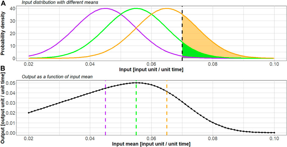
Figure 1. (A) Gaussian input distributions for three different means (0.045, 0.055, and 0.065 input units per unit time, respectively) and a cut-off threshold of 0.070 input units per unit time; (B) output as a function of the input mean (i.e., average production level) given a Gaussian input distribution with a standard deviation of 0.01 input units per unit time.

1.2 Research goals

The goals of this investigation are: 1) The authors introduce the basic notion of threshold-impeded stochastic production systems. 2) The authors show that these systems display a non-monotonous relationship between the production output and the average input level (representing the resource load at which the production system is run). This relationship is a universal feature of such TISP systems. 3) The authors offer a method to assess the output sensitivity of TISP systems in response to varying system and input parameters. 4) The authors illustrate applicability of this theoretical concept to real-life systems through two application scenarios which both fall into the category of TISP systems.

1.3 Application scenarios

TISP systems can be found in diverse industrial contexts such as the continuous casting of steel and the generation of electric power through wind turbines. For example, if a continuous caster operates so fast that the mass flow of manufactured steel outruns the supply of liquid steel, the entire casting procedure needs to be interrupted for maintenance (Merten et al., 2022b). Analogously, wind turbines have to be switched off during stormy weather, or else they will possibly suffer structural damages (Klimstra and Hotakainen, 2011). The idea behind choosing two vastly different application scenarios is to emphasise the wide-ranging applicability of TISP concepts.

1.4 Approach

The authors intend to approach the TISP-inherent optimization problem by abstracting real-life nonlinear systems into minimal models (Batterman and Rice, 2014), capturing the “stylized facts” of the production mechanisms and then revealing, via careful numerical analysis, the influencing factors that allow an accurate control of the system. The study of nonlinear dynamics has a long tradition of contributing to a better understanding of phenomena in industrial production, assembly and supply systems (Chankov et al., 2016; Alkan et al., 2018; Chankov et al., 2018; Lin and Naim, 2019).

The stylized representation of TISP systems allows one to define TISP subtypes, which lead to various input-output relationships and sensitivities with respect to noise types. To this end, the authors consider the output of TISP systems that exhibit typical nonlinear transformations, as sketched in Figure 2. Depending on the application scenario, three TISP subtypes are distinguished (i) standard TISP: The nonlinearity of the system (i.e., the threshold): brings excess input values down to zero (see Figure 2B); (ii) penalized TISP: The nonlinearity brings excess input values to a value below zero (see Figure 2C); (iii) lagged recovery TISP: After excess input values are reduced, the system is unable to produce further output for a certain number of time steps (see Figure 2D).

Figure 2

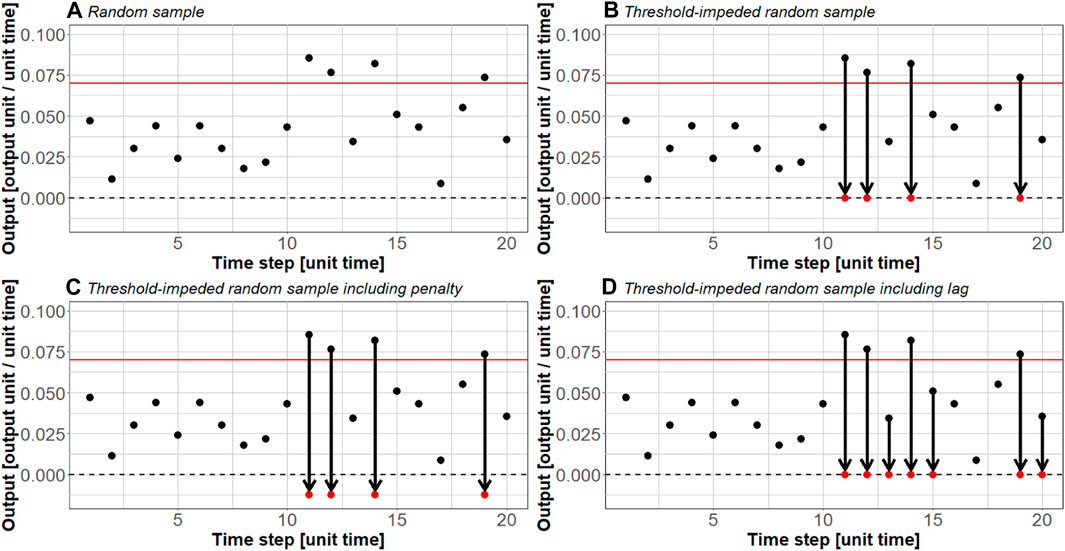
Figure 2. Examples of generic TISP subtypes; (A) 20 time steps of uniformly distributed random input values; the input values are processed by a threshold device acting as a nonlinear transformation (i.e., (B) standard TISP, (C) penalized TISP, or (D) lagged recovery TISP).

In order to provide a quantitative relationship between the generic TISP systems (i.e., standard, penalized, or lagged recovery) and the application scenarios outlined above, the authors estimate the systems’ output (i.e., steel mass flow and electric power) by simulating and transforming random input values from several probability models (e.g., uniform or Weibull noise) as well as computing expected values numerically. Since these expected values originate in output integrals of the minimal models, it is shown how the models compare against the simulated outputs. Then, varying the average input level enables one to determine the maximally achievable output and its corresponding parameter values. This procedure is repeated numerous times subject to changing statistical features of the noisy input (e.g., distribution width) and other experimental parameters (e.g., penalty and lag size) which reveals how sensitive the system output is to such adjustments. For the continuous casting application, the authors also examined time-correlated input from an Ornstein-Uhlenbeck process that experiences a lagged recovery nonlinearity (see Figure 2D). Contrasting the mean-reversing behavior of an Ornstein-Uhlenbeck process with uncorrelated Gaussian input will demonstrate the impact of noise correlations on the production performance.

1.5 Novelty

To the authors’ best knowledge, the category of TISP systems has not been described before. Understanding such high-level categories can be helpful for production planning and control, where the resource load either can be selected or the system can be set up to perform optimally at typical input levels, and for a more detailed modeling of specific systems. For such modeling efforts, the authors argue that in any TISP system, non-monotonous input-output relationships will be encountered independent of the intricacies of the mathematical or computational model.

1.6 Outline

The remainder of this article is organized in the following way: First, the authors present selected works revolving around uncertainty in production systems and they point out in what sense this study fits into the research landscape (Section 2). Section 3 (“Application scenarios”) explains the production mechanisms and input distributions behind the two scenarios, i.e., steel continuous casting and wind power generation. Once the underlying production mechanism has been understood, the authors establish the expected value integrals that describe the output of the various TISP system subtypes (see Section 4 “Minimal models”). In Section 5, the Ornstein-Uhlenbeck process for time-correlated input values is introduced which becomes useful in the case of the lagged recorvery TISP system (see Figure 2D). Section 6 (“Methods”) discloses the simulation framework and it reveals how the minimal models as well as the respective system or input parameters are deployed to assess the output sensitivity of TISP systems. Throughout Section 7, the numeric and simulation results are presented and discussed before, finally, in Section 8 the authors conclude the findings and give an outlook on promising future research directions.

2 Related work

2.1 Control and flexibility

In response to uncertainty, Correa (1992) offers two remedies, namely, control and flexibility. “Control” includes all efforts that aim at proactively reducing uncertainty before it arises, whereas “flexibility” stands for reactively coping with uncertainty after it has arisen. Angkiriwang et al. (2014) compare the usage of reactive uncertainty strategies such as buffering and proactive uncertainty strategies such as redesigning. However, buffering will not have the desired effect if the interplay between uncertain production inputs and TISP thresholds complicates the determination of appropriate buffer strategies. Similarly, redesigning the production process will not reduce uncertainty if the production process cannot be redesigned further due to technology and cost restrictions or saturation effects.

Sreedevi & Saranga, (2017) state that flexibility helps “in reducing […] supply and manufacturing process risks” but the “effect is context-dependent.” As a solution to this, the authors offer a generalized description of uncertainty in threshold-impeded production systems that can be adapted to different contexts (the only condition being that the production mechanism itself is understood and can be modelled mathematically). Regardless of whether common control or flexibility strategies are applicable, this description deepens the understanding of production outputs and their sensitivity to uncertain inputs.

2.2 Rescheduling

Production uncertainty can be combatted reactively through rescheduling (Vieira et al., 2003; Psarommatis et al., 2021). Rescheduling has a long history in the steel industry; especially multi-agent systems were often used for this purpose (Cowling et al., 2003; Cowling et al., 2004; Ouelhadj et al., 2004). More recently, evolutionary algorithms (Guo and Tang, 2019; Merten et al., 2024) and machine learning (Iglesias-Escudero et al., 2019; Li et al., 2020) have become the preferred solutions. However, all of these solutions are extremely context-dependent and they are invalid with respect to other application scenarios such as wind turbines. As stated above, this is something the authors try to avoid with the TISP approach.

2.3 Buffering and diversification

In the context of wind turbines, a common “buffering” strategy comprises changing the orientation of the wind turbine rotor blades with respect to the direction from which the wind is blowing. So, one can either harness more energy by aligning the rotor blades with the wind or protect the wind turbine from strong winds by turning the rotor blades away from the wind input direction (Castellani et al., 2015; Yan, 2015). Nevertheless, this is only feasible for rather small variations in the wind speed and, again, this strategy is highly context-dependent.

On top of that, to reduce the power output variability of wind farms, diversification methods could be applied. For instance, spatially distributing wind turbines over a given area (Cassola et al., 2008) or combining different types of wind turbines (e.g., smaller turbines for weaker winds and larger turbines for stronger winds) helps to reduce variability. One a higher level, it is even feasible to interconnect entire wind farms (Archer and Jacobson, 2007; Katzenstein et al., 2010). While these diversification methods are to some extent adaptable to other application scenarios such as steel continuous casting, they primarily aim at only reducing the output variability but not at maximizing the overall output. Nevertheless, output maximization is “usually one of the most important objectives for any [wind farm] designer” because it is closely linked to the revenue of a wind farm company (Feng and Shen, 2017). On the contrary, maximizing the overall output is the central purpose of the TISP approach as explained in the introduction of this article.

In steel continuous casting, the tundish (which is a reservoir of molten steel; see Section 3) may serve as a buffer containment. Therefore, it can be used to slightly slow down or ramp up the production process. Yet, the tundish’s ability to combat uncertainty is limited because changing the flow pattern of the molten steel has profound effects on the steel quality (Zhong et al., 2007). Besides, one has to consider a multitude of constraints when adjusting the casting speed or else the resulting steel strand might be torn apart or it might not be sufficiently solidified before leaving the production machine (Merten et al., 2022b). Both these occurrences would cause the production to halt for cost- and time-intensive maintenances.

2.4 Modernization

A proactive way to reduce uncertainty is to modernize the production environment (Gerwin and Tarondeau, 1982; Ettlie, 1990; Groover, 2006; Bertsimas and Thiele, 2014; Dotoli, et al., 2019; Ghobakhloo, 2020). For this purpose, Industry 4.0 technologies such as cyber-physical systems (CPS), internet of things (IoT), artificial intelligence (AI), and cloud computing (Zhong et al., 2017; Xu et al., 2018; Oztemel and Gursev, 2020) are routinely implemented. In particular, AI applications have proven valuable as means to combat production uncertainty (Iglesias-Escudero et al., 2019; Arinez et al., 2020). For example, Roy et al. (2004) describe an inference model that is capable of handling schedule disturbances in steel production. With respect to wind turbine control and optimization, neural networks are frequently utilized (Chatterjee and Dethlefs, 2021). But what is to be done in production environments where access to advanced technologies is limited or the necessary input data does not exist (Lee et al., 2013)? In fact, many steel factories still fall under this category. For these situations, the authors offer a technique that, instead of focusing on individual input events or threshold violations, yields universal recommendations which work very well on average.

2.5 Analytical models and simulation

On a more theoretical level, Peidro et al. (2009) suggested analytical models and simulations (Aouam et al., 2018; Jamalnia et al., 2019; Gupta and Maravelias, 2020; Tordecilla et al., 2021). Simulation tools have been successfully deployed to tackle uncertainty in production systems (Negahban and Smith, 2014; Jeon and Kim, 2016; Zhang et al., 2019) because “due to [their] low cost, quick analysis, low risk and meaningful insight that [they] may provide” (Mourtzis, 2020) simulation tools allow “for the experimentation and validation of […] process and system design” (Mourtzis et al., 2014) and show “unique advantages in solving practical problems” (Zhang et al., 2019). Nevertheless, a few research gaps concerning state-of-the-art simulation tools have been identified: (i) Capable tools only exist for a selective subset of application scenarios (Mourtzis et al., 2014) and (ii) “unified approaches and terminology” are missing (Mourtzis, 2020). As a solution to this, the methodology can be viewed as a simulation toolbox that is adaptable to diverse application scenarios and, regardless of the scenario, always follows the same underlying recipe or approach.

3 Application scenarios

3.1 Steel continuous casting

Over the past 70 years, continuous casting has widely replaced ingot casting as the primary fabrication method for steel slabs (Santos et al., 2003). The working principle of a continuous caster is shown in Figure 3. First, the steel alloy is poured into the tundish from which it passes through a mold. Here, the tundish serves as a funnel and buffer containment that ideally ensures a constant delivery of liquid metal. The design of the mold basically dictates the shape and proportions of the emerging steel slabs, while the amount of steel flowing across the mold can be modified with the help of a nozzle. At the mold exit, the nascent steel slabs are still largely molten, and secondary cooling in the form of water sprays has to be carried out for further shell solidification (Irving, 1993).

Figure 3

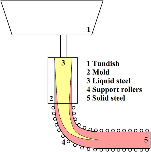
Figure 3. Steel slab production through continuous casting; the liquid (solid) steel is colored yellow (red); abstracted from Louhenkilpi, 2014.

Extensive attempts have been made to increase the operating speed of casters and, therefore, their output. Faced with the ubiquitous compromise between output maximization (Li and Thomas, 2000) and process quality/steadiness, numerous researchers have examined likely limitations of the operating speed (Merten et al., 2022b) which, among others, encompass several customer-dependent slab properties (e.g., slab dimensions). For instance, to ensure sufficient shell solidification the operating speed has to be chosen so that the slabs have enough time to solidify. This solidification time is tightly linked to one of the most important planning parameters in steel production (Özgür et al., 2021), namely, the slab thickness (Thomas, 2002). In practice, it is often not possible to maintain a constant operating speed which would be beneficial for the slab quality (Zhang et al., 2006; Wang and Zhang, 2010; Zhang and Wang, 2010) since subsequently manufactured customer orders typically exhibit divergent thickness values.

Another example shedding light onto the output maximization trade-off is discussed in Merten et al. (2022b). The authors inspected historical production data from an industrial casting machine which revealed an abrupt adjustment of the casting speed strategy and, subsequently, they traced this regime transition back to the existence of a theoretical limit for the maximum achievable steel mass flow. In essence, this maximum achievable steel mass flow is motivated by the fact that the tundish (see Figure 3) must not run out of liquid steel. As soon as the steel mass flow (and, hence, the operating speed) exceeds this maximum limit, the continuous casting process has to be stopped for cost-intensive and time-consuming maintenance during which no output can be generated.

In this application scenario, the system’s input uncertainty originates from complex planning constraints (Merten et al., 2022a) as well as unstable customer demand entailing fluctuations of the casting speed-relevant variables. At the same time, a threshold/nonlinear transformation is imposed by the maximum achievable steel mass flow beyond which the steel slab might be torn apart (Merten et al., 2022b). These systemic features turn the continuous casting of steel into a TISP device.

3.2 Wind turbines

Wind turbines play an important role in today’s renewable energy market (Liu et al., 2013; Wood et al., 2013). By means of rotor blades and an electric generator, they convert wind kinetic energy into electric energy, where the relationship of the wind speed $v$ (unit: $\mathrm{m}/\mathrm{s}$) and the generated electrical power $P$ (unit: $\text{kg}\times {\mathrm{m}}^2/{\mathrm{s}}^3$) is demonstrated to be cubic (Bergey, 1979; Salameh and Safari, 1992):

$P=\frac{\rho A{v}^3}{2},$

where $\rho$ and $A$ denote the air density (unit: $\text{kg}/{\mathrm{m}}^3$) and the rotor blade swept area (unit: ${\mathrm{m}}^2$). Typically, wind turbines are characterized by three different thresholds on the wind speed (i.e., cut-in, rated and cut-out speeds) that govern the transformation from wind to energy. At speeds below the cut-in threshold $v_{in}$, no electric energy is built up because of static friction between the mechanical components of the wind turbine and negligible torque on the rotor blades (Wood et al., 2013). Above the cut-in speed, the electric energy production grows substantially with the wind speed; however, wind turbines are constructed to trim any energy surpluses beyond a rated threshold $v_r$ corresponding to the maximum capacity of the integrated electric generator (Manwell et al., 2010; Wood et al., 2013). Moreover, wind turbines need to be protected against storms as pointed out earlier. Thus, they are shut down as soon as the wind speed surpasses a specified cut-out threshold $v_{out}$ (Klimstra and Hotakainen, 2011). The impact of the wind intensity on the electric power output is commonly documented in power curves (Carrillo et al., 2013; Hau, 2013). A schematic illustration of such a power curve is shown in Figure 4 (Salameh and Safari, 1992). In the theoretical framework, the wind corresponds to the stochastic input, whereas the wind turbine and its speed thresholds act as a nonlinear transformation. Based on these technological aspects, the authors stylize the functioning of a wind turbine as a TISP system and they utilize various minimal models (see Section 4) to study how wind turbine parameters as well as the wind speed pattern affect the turbine performance.

Figure 4

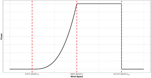
Figure 4. Typical power curve relating the wind speed to the power output of a wind turbine (Salameh and Safari, 1992); it exhibits three thresholds: cut-in, rated and cut-out speeds.

From the principles of fluid flow, Lanchester and Betz have deduced a physical boundary for the maximum energy that can be obtained through wind turbines (Bergey, 1979). More recently, the literature concerning wind energy mainly addressed two distinct research topics—(i) the fitting of stochastic distributions to wind speed data (Morgan et al., 2011) and (ii) the analysis of technical details of wind turbines (Carrillo et al., 2013)—with some articles considering both jointly (Kwon, 2010; Liu et al., 2013). While Morgan et al. (2011) explore the suitability of theoretical wind speed models with regards to offshore wind measurements, Carillo et al. (2013) evaluate a series of generic equations to approximate the conversion of wind to energy via wind turbines. Stevens and Smoulders (1979) observe the energy production as a function of the Weibull distribution shape parameter (whereby the Weibull distribution is the most commonly used distribution to characterize wind speeds). Furthermore, frameworks that enable one to match wind turbines to wind speed distributions/wind sites are provided by Salameh and Safari (1992)/Ritter and Deckert (2017). Here, the authors intend to expand previous methodologies through additional TISP features such as penalties and lagged recoveries.

4 Minimal models

In order to assess the parameter sensitivity of a TISP system on the output performance $Y$, minimal models are developed that quantitatively explain the transformation process undergone by the noisy input $X$. Successively, the authors consider the three generic TISP systems already mentioned (i.e., standard, penalized and lagged recovery) and their application to steel continuous casting and wind power generation. When uncorrelated over time, the noisy input per unit time is fully described by an independently distributed random variable $X$ with the probability density $f\left(x\right)$. The case of a time-correlated input $X\left(t\right)$ requires the framework of special stochastic processes such as the Ornstein-Uhlenbeck process (see Section 5).

Standard TISP system (uncorrelated noisy input; both application scenarios): In the case of standard TISP systems, the predicted average outcome per unit time Y can be computed via the expected value $E\left[g\left(X\right)\right]={\int }_0^{\infty }g\left(x\right)f\left(x\right)dx$, as done in Bendat and Piersol (2011). The modelling step lies in devising the appropriate transformation $g\left(\bullet \right)$ of the input $X$, such that $Y=g\left(X\right)$. In particular $g\left(\bullet \right)$ involves the threshold(s) controlling the functioning of the TISP system and the accompanying nonlinear transformation(s) of the input.

In the case of steel continuous casting, there is only one upper threshold T, corresponding to the maximum mass flow (i.e., mass per unit time) above which the machine must stop (Merten et al., 2022b). When the system operates below the threshold, the output is equal to the input, therefore $g_{steel}\left(X\right)=X{\mathbf{1}}_{\left[0,T\right]}\left(X\right)$. On average, it becomes:

$E\left[Y_{steel}=g_{steel}\left(X\right)\right]={\int }_0^{T}xf\left(x\right)dx$

In the case of a wind turbine, the power curve depicted on Figure 4 leads to:

$E\left[Y_{wind}=g_{wind}\left(X\right)\right]\propto {\int }_{v_{in}}^{v_r}{x}^{3}f\left(x\right)dx+v_r^3{\int }_{v_r}^{v_{out}}f\left(x\right)dx$

where $v_{in}$, $v_r$, and $v_{out}$ are the cut-in, rated and cut-out speeds, respectively (Wood et al., 2013). The function $g_{wind}\left(X\right)$ involves these three thresholds and the above-mentioned cubic relationship between the wind speed and the generated power $P=\rho A{v}^3/2$ (Bergey, 1979; Salameh and Safari, 1992), namely, $g_{wind}\left(X\right)=\left(\rho A/2\right)\left[X^3{\mathbf{1}}_{\left[v_{in},v_r\right]}\left(X\right)+v_r^3{\mathbf{1}}_{\left[v_r,v_{out}\right]}\left(X\right)\right]$.

Note that in both application scenarios (steel continuous casting and wind power generation), the simulation of the TISP system amounts to computing $g\left(x\right)$ for each sampled value $x$ of the noisy input (sampled according to the prescribed distribution $f\left(\bullet \right)$); therefore, the set of simulated outcomes corresponds to a sampling of the above expected value $E\left[Y_{steel}\right]orE\left[Y_{wind}\right]$. If real-life production data was available (i.e., input and output data), this data could be used to configure the minimal model and test its suitability.

Penalized TISP system (uncorrelated noisy input, both application scenarios): In penalized TISP systems, overshooting the upper threshold (T or $v_{out}$) leads to a negative outcome $-p$, mimicking situations where some of the production output has to be discarded. Specifically, such a penalty could arise in the two application scenarios considered here for the following reasons: 1. If the continuous casting process needs to be rebooted after an abrupt cast break, some of the initial yields may have to be disregarded until the caster reaches steady manufacturing conditions. 2. In order to shut down/start up a wind turbine due to a storm, some electrical power will be required which consequently cannot be fed into the grid. For the continuous casting system, this effect is taken into account by adding a penalty term $-p_{steel}{\mathbf{1}}_{\left]T,\infty \right]}\left(X\right)$ to the above-mentioned function $g_{steel}\left(X\right)$, which leads to a new formula for the average output per unit time:

$E\left[Y_{steel}\right]={\int }_0^{T}xf\left(x\right)dx-p_{steel}{\int }_T^{\infty }f\left(x\right)dx$

Similarly, for the wind power application scenario, a term $-p_{wind}{\mathbf{1}}_{\left]v_{out}\left.,\infty \right]\right.}\left(X\right)$ is added to the above-mentioned function $g_{wind}\left(X\right)$ so that the average output turns out to be:

$E\left[Y_{wind}\right]\propto {\int }_{v_{in}}^{v_r}{x}^{3}f\left(x\right)dx+v_r^3{\int }_{v_r}^{v_{out}}f\left(x\right)dx-p_{wind}{\int }_{v_{out}}^{\infty }f\left(x\right)dx$

Lagged recovery TISP system (uncorrelated noisy input, both application scenarios): The authors also consider the possibility that resetting the TISP system after overshooting the upper threshold takes some time, say, $l$ production time steps. Additional threshold violations during this lag result in repeated shutdowns and delay the moment when the production resumes (i.e., after $l$ time steps without exceeding the threshold).

The authors denote $F_X$ the cumulative distribution of the random variable $X$, namely, $F_X\left(T\right)$ is the probability that the input $X$ lies below $T$ during the considered time step. In the absence of time correlations, the condition that the input does not overshoot the threshold $T$ during $l$ time steps is taken into account through a multiplicative factor ${\left[F_X\left(T\right)\right]}^l$. For the two application scenarios this yields:

$E\left[Y_{steel}\right]={\left[F_X\left(T\right)\right]}^l{\displaystyle \underset{0}{\overset{T}{\int }}}xf\left(x\right)dx$

$E\left[Y_{wind}\right]\propto {\left[F_X\left(v_{out}\right)\right]}^l\left[{\displaystyle \underset{v_{in}}{\overset{v_r}{\int }}}{x}^{3}f\left(x\right)dx+v_r^3{\displaystyle \underset{v_r}{\overset{v_{out}}{\int }}}f\left(x\right)dx\right]$

Note that in this case, the output $Y$ is not related in a simple way to the input $X$, i.e., it is no longer possible to write $Y=g\left(X\right)$ since the output depends on several preceding input steps. However, when the input is not time-correlated (as in this case) this phenomenon is already reflected in the average output value given above.

Combination of penalized and lagged recovery TISP system (uncorrelated noisy input; both application scenarios): Barring any time-correlated inputs, the lagged recovery TISP system can adopt penalized TISP features through (i) the addition of a term $-p{\mathbf{1}}_{\left]T,\infty \right]}\left(X\right)$ to the production event occurring after $l$ steps and (ii) the contribution of a penalty $p$ (with probability $1-{\left[F_X\left(T\right)\right]}^l$) in case of a shutdown event occurring during these $l$ steps:

$E\left[Y_{steel}\right]={\left[F_X\left(T\right)\right]}^l\left[{\displaystyle \underset{0}{\overset{T}{\int }}}xf\left(x\right)dx-p_{steel}{\int }_T^{\infty }f\left(x\right)dx\right]-p_{steel}\left(1-{\left[F_X\left(T\right)\right]}^l\right)$

$E\left[Y_{wind}\right]\propto {\left[F_X\left(v_{out}\right)\right]}^l\left[{\displaystyle \underset{v_{in}}{\overset{v_r}{\int }}}{x}^{3}f\left(x\right)dx+v_r^3{\displaystyle \underset{v_r}{\overset{v_{out}}{\int }}}f\left(x\right)dx-p_{wind}{\int }_{v_{out}}^{\infty }f\left(x\right)dx\right]-p_{wind}\left(1-{\left[F_X\left(v_{out}\right)\right]}^l\right)$

Lagged recovery TISP system (correlated noisy input; steel continuous casting only): Time-correlated inputs only matter when some integration over multiple time steps occurs in the production process. In lagged recovery TISP systems, the sequence of input values during $l$ steps and its joint probability has to be taken into account. To be specific, the authors detail the computation for the continuous casting system: The output $Y_t$ at time $t$ depends on the inputs at times $t$, $t-1$, $\dots$, $t-l$. Computing its averages involves the joint probability of $X_t$, $X_{t-1}$, $\dots$, $X_{t-l}$, through the joint density $f\left(x,x_1,\dots ,x_l\right)$. The authors introduce the conditional density depending on the preceding $l$ input values:

$f\left(x,x_1,\dots ,x_l\right)=f\left(\left.x\right|x_1,\dots ,x_l\right)\times f\left(x_1,\dots ,x_l\right)$

The average output for the continuous casting application scenario can then be expressed as

$E\left(Y_t\right)={\int }_0^T\dots {\int }_0^{T}d{x}_1\dots d{x}_{l}f\left(x_1,\dots ,x_l\right)\times {\int }_0^{T}xf\left(\left.x\right|x_1,\dots ,x_l\right)dx$

where the contribution ${\int }_0^T\dots {\int }_0^{T}d{x}_1\dots d{x}_{l}f\left(x_1,\dots ,x_l\right)$ is simply equal to ${\left[F_X\left(T\right)\right]}^l$ in the absence of time correlations. The wind turbine scenario is not considered for this kind of TISP system due to the increased mathematical complexity that comes with the addition of time correlations to the output model.

5 Ornstein-Uhlenbeck (OU) process

A standard framework for modeling the noisy input of TISP systems is that of stochastic processes, in particular the Ornstein-Uhlenbeck process for the case of a time-correlated input. The latter is a stochastic process $X_t$ $\left(t>0\right)$ defined by the stochastic differential equation $d{X}_t=\theta \left(\mu -X_t\right)dt+\sigma d{W}_t$ where $\mu$ is the theoretical mean of the process (computed as the long-run empirical mean) and $\theta$ is called the stiffness (or the rate of mean reversion), while $\sigma$ denotes the diffusion coefficient (also termed volatility) and $W_t$ is a standard Wiener process (Maller et al., 2009). As opposed to standard Brownian motion, an OU-particle (i.e., a particle whose motion $X_t$ follows an OU-process) converges towards a constant level $\mu$ by drifting upwards whenever $X_t<\mu$ and downwards whenever $X_t>\mu \left(Uhlenbeck\&Ornstein,1930\right)$. Aside from statistical physics, OU-variants were adopted in financial mathematics (Vasicek, 1977) and neuroscience (Ricciardi and Sacerdote, 1979; Laing and Lord, 2010). In the context of this article, OU-processes can be viewed as analogous to production environments with implicit mean-reverting features. Such features could manifest themselves, for instance, through system operators that meticulously attempt to counterbalance fluctuations in the production process.

Ornstein and Uhlenbeck (1930) have proven that the motion of OU-particles is normally distributed; Hence, expressions for the mean and covariance function of an OU-process are easily derived (Maller et al., 2009). An OU-process $X_{\tau }$ with start value $X_0$ has mean $X_0\times \mathit{exp}\left(-\theta t\right)+\mu \left(1-\mathit{exp}\left(-\theta t\right)\right)$ and variance $\left({\sigma }^2/2\theta \right)\times \left(1-\mathit{exp}\left(-2\theta t\right)\right)$:

$X_t\sim N\left(X_0\times \mathit{exp}\left(-\theta t\right)+\mu \left(1-\mathit{exp}\left(-\theta t\right)\right),\frac{{\sigma }^2}{2\theta }\left(1-\mathit{exp}\left(-2\theta t\right)\right)\right)$

Besides, Gillespie (1996) contributes an efficient algorithm for the simulation of the position and velocity of OU-particles. Special interest was shown in the question at what time an OU-particle exceeds a given distance $S$ from its equilibrium position (Thomas, 1975; Cerbone et al., 1981; Alili et al., 2005). The mean, variance, and skewness of this so-called hitting time are disclosed in Cerbone et al. (1981). For an OU-process starting at its theoretical mean $\mu$, they report the mean hitting time $H$ as (Cerbone et al., 1981):

$H\left(S|\theta ,\mu ,{\sigma }^2\right)=\frac{1}{2\theta }{\displaystyle \sum _{n=1}^{\infty }}\frac{{\left(\sqrt[2]{\frac{2\theta }{{\sigma }^2}}\left(S-\mu \right)\right)}^{2n}}{n\left(2n-1\right)‼}+\sqrt[2]{\frac{\pi }{{\theta \sigma }^2}}\left(S-\mu \right){\displaystyle \sum _{n=0}^{\infty }}\frac{{\left(\sqrt[2]{\frac{2\theta }{{\sigma }^2}}\left(S-\mu \right)\right)}^{2n}}{2^{n}n!\left(2n+1\right)}$

During the numerical experiments of output performance, the authors use this mean hitting time as the simulation length for the OU-process (see Sections 6 and 7).

Note that such time-correlated input processes only impact the output productivity in the case of a lagged recovery TISP system (see Figure 2; Section 4). Apart from an OU-process, the authors could have chosen any other type of time-correlated input but they wanted to deploy a stochastic process for which the probability density can be written in terms of elementary functions. This will be helpful with regards to the minimal models presented in Section 4.

6 Methods

As stated earlier, the goal is to investigate the output sensitivity of TISP systems to changing process parameters through minimal models (see Section 4) and simulations. The output simulations are achieved by creating input samples with the desired type/extent of randomness and subsequently transforming them through the TISP system. For comparison reasons, the output integrals from Section 4 are numerically integrated and held against these output simulations.

Based on regression methods, the authors then investigate the optimal output’s dependence on tunable process parameters. Here, the distribution width $w$/shape $k$, the penalty $p$, and the recovery lag $l$ can be varied as well as the kind of noisy input, as described by the probability density $f\left(x\right)$. First, the authors consider uncorrelated input, then a lagged recovery TISP model fueled by correlated Ornstein-Uhlenbeck noise. The latter TISP model is only deployed in the continuous casting of steel scenario, whereas the experiments for uncorrelated noise apply to both real-life scenarios.

6.1 Uncorrelated noisy input (both application scenarios)

For both application scenarios–the continuous casting of steel and the generation of power via wind turbines–the authors choose the input probability distributions according to the pertaining literature and industrial data. A summary of all distributions is presented in Table 1 and an explanation for their parameters is enclosed in Table 2. Moreover, Table 2 indicates the range of the noise parameter values in the numerical experiments.

Table 1

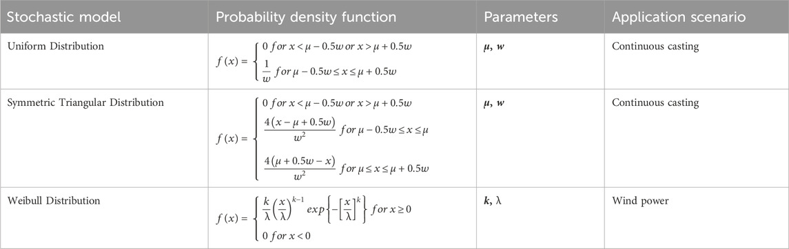
Table 1. Noise types.

Table 2

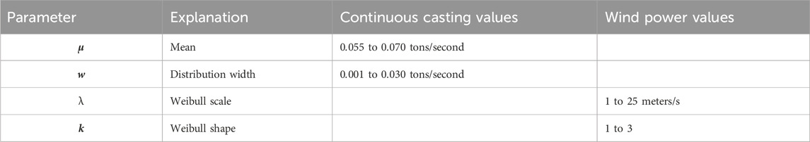
Table 2. Noise parameters.

As can be seen in Table 1, the authors characterize the mass flow data (Merten et al., 2022b) by uniform and symmetric triangular distributions, while wind speeds are most commonly reproduced by Weibull distributions (Stevens and Smulders, 1979). The mean steel mass flow as well as the scale of the wind speed distribution are varied between $0.055$ and $0.070$ tons per second as well as $1.00$ and $25.00$ meters per second, respectively (see Table 2). Also, the authors select the threshold wind speeds $v_{in}$, $v_r$, $v_{out}$ as reported in Carillo et al. (2013) and the maximum possible steel mass flow $T$ according to Merten et al. (2022b). The cut-off thresholds $T$ and $v_{out}$ are fixed at $0.070$ meters per second and $27.00$ meters per second (see Table 3), respectively.

Table 3

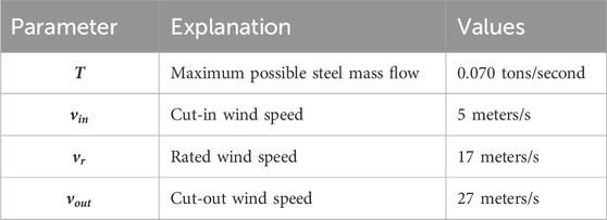
Table 3. Threshold parameters.

After studying the discrepancy between the numerical integration and the simulations, the authors determine, by means of regression, the position of the performance maximum as a function of the noise parameters $w$/$k$, the penalty $p$, and the lag $l$. For this purpose, the “combination of penalized and lagged recovery TISP” system (see Section 4) is implemented as a minimal model because it embeds the “standard TISP” system ($p=l=0$), the “penalized TISP” system ($l=0$), and the “lagged recovery TISP” system ($p=0$) in its limits.

6.2 Time-correlated noisy input (steel continuous casting only)

Next, the effects of input correlations on the output productivity of a lagged recovery TISP system (lag $l=1$) are examined (see Section 4) with respect to the continuous casting application scenario. To this end, the authors use correlated noise from an Ornstein-Uhlenbeck process and white Gaussian noise as a baseline comparison. The distribution mean $\mu$ varies from $0.055$ to $0.070$ tons/second, whereas the standard variation $\sigma$ changes between $0.001$ and $0.030$ tons/second. The OU-specific parameters are located between $2$ and $10$ (for the stiffness $\theta$) as well as $0.055$ and $0.070$ tons/second (for the theoretical mean $\mu$/start value $x_0$), respectively. For both types of input fluctuations, the authors assume the same threshold parameter as in the previous subsection (see Subsection 6.2).

For the simulation of the OU-process starting at a start value $X_0$ equal to its theoretical mean $\mu$, the process’ mean hitting time $H$ (Cerbone et al., 1981) is adopted as the simulation length. Through Bland-Altman diagrams (Bland and Altman, 1986), the authors assess the validity of the hitting time formula (see Section 5) by comparing it with the average time span that a simulated OU-process needs to exceed a given distance from its equilibrium mean. Bland-Altman diagrams plot the difference between two measurement series against the (arithmetic) average of the two series; they visualize to what degree the series deviate from each other through the indication of confidence intervals. Afterwards, the minimal model for time-correlated input (see Section 4) is held against the output simulations (obtained by transforming a random OU-sample according to the cut-off threshold $T$). Finally, the authors measure the impact of the noise parameters (i.e., standard deviation and stiffness) on the position of the performance maximum by using regression methods.

7 Results and discussion

7.1 Uncorrelated noisy input (both application scenarios)

7.1.1 Steel continuous casting

As can be seen in the quantile-quantile plots shown in Figure A.1 (see Supplementary Material A), the fluctuations of the input mass flow in Merten et al. (2022b) are described by uniform and symmetric triangular distributions to an adequate extent. Figure 5 and A.2 demonstrate the perfect agreement of the minimal model and the simulations for these two distributions. While the size of the penalty or the lag do not seem to affect the position of the maximum output with respect to the distribution mean (see Supplementary Material A: Figure A.2), the distribution width does have a substantial effect. In the selected parameter ranges, the relationship between the value of the distribution mean at which the maximum performance occurs and the distribution width turns out to be linear (see Supplementary Material A: Figure A.3). Once an optimum has been reached, the output curve drops off more sharply for the uniform distribution than for the symmetric triangular distribution. This happens since, for uniformly distributed input samples, a much larger part of the area under the probability density curve is located beyond the threshold compared to the symmetric triangular distribution (given the same distribution mean $\mu$ and width $w$). Hence, system operators adjusting the process parameters would have to be more careful when facing uniformly distributed input. Furthermore, for longer lags both mass flow curves lose their concavity as the performance approaches zero (see Supplementary Material A: Figure A.2). The findings underscore the relevance of this numerical experiment because, e.g., in the case of a uniform noise distribution, overshooting the optimal average production level by less than eight percent may lead to a production loss that is greater than 23 percent (see Figure 5A).

Figure 5

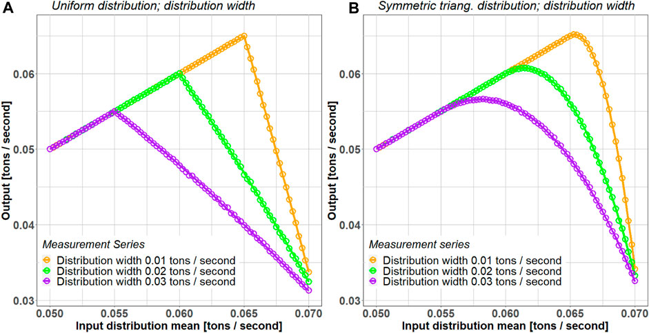
Figure 5. Output mass flow as a function of the mean of the mass flow input distribution for various input distribution widths for the (A) uniform distribution (distribution width $\mathrm{w}=0.01$ to $0.03$ tons/second; penalty $\mathrm{p}=0.00$ tons/second; lag $\mathrm{l}=0$ time steps) and the (B) symmetric triangular distribution (distribution width $\mathrm{w}=0.01$ to $0.03$ tons/second; penalty $\mathrm{p}=0.00$ tons/second; lag $\mathrm{l}=0$ time steps); for each set of parameters the results of the minimal models (continuous lines) and the simulations (circles) are presented.

7.1.2 Wind turbines

In Figure 6, the authors describe the wind power production as a function of the Weibull distribution scale $\mathrm{\lambda }$ subject to varying distribution shape $k$, penalty $p,$ and lag $l$. Again, the minimal models agree with the results of the simulations. However, in this case, the position of the maximum output is impacted by the size of the penalty and the duration of the lag. Apparently, the distribution scale optimizing the wind power generation roughly depends on the square of the penalty and the logarithm of the lag (see Supplementary Material A: Figure A.4). Besides, the authors observe that longer lags again induce a shift of curvature from concave to convex for larger Weibull scale (see Figures 6B, C). Assuming Weibull-distributed wind speeds, the planners of wind farms have to consider threshold-induced power losses (“penalty”) and downtimes (“lag”) when choosing the wind speed pattern (i.e., the farm site). Exceeding the optimal distribution scale by approximately 21 percent might bring a power loss of almost one-third.

Figure 6

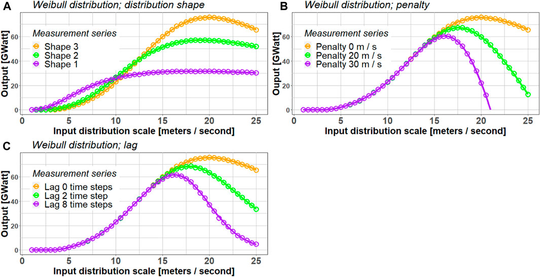
Figure 6. Output wind power as a function of the scale of the wind speed input distribution under changing (A) distribution shape (distribution shape $\mathrm{k}=1$ to $3$; penalty $\mathrm{p}=0$ meters / second; lag $\mathrm{l}=0$ time steps), (B) penalty size (distribution shape $\mathrm{k}=3$; penalty $\mathrm{p}=0$ to $30$ meters / second; lag $\mathrm{l}=0$ time steps), and (C) lag duration (distribution shape $\mathrm{k}=3$; penalty $\mathrm{p}=0$ meters / second; lag $\mathrm{l}=0$ to $8$ time steps) for the Weibull distribution; for each set of parameters the results of the minimal models (continuous lines) and the simulations (circles) are presented; the power values (y-axis) were obtained by assuming an air density of $\mathrm{\rho }=1.225\text{kg}/{\mathrm{m}}^3$ and a rotor blade radius of $\mathrm{r}=100$ m.

7.2 Time-correlated noisy input (steel continuous casting only)

Earlier, the authors have established the mean hitting time of an Ornstein-Uhlenbeck process (see Section 5). In Figure 7, the analytical formula from Cerbone et al. (1981) is compared with the average time span that a simulated OU-process needs to surpass a given threshold, by looking at how much the simulation deviates from the analytical hitting time. If the cut-off threshold is chosen to be $0.070$ tons per second and change theoretical mean $\mu$ (and with it the starting value $x_0$) from $0.055$ to $0.070$ tons per second, the formula predicts the hitting time fairly well for values up to 40 time steps. This is confirmed by the corresponding Bland-Altman diagram (Bland and Altman, 1986; see Supplementary Material A: Figure A.5) as the deviation between the two series of measurements exceeds the confidence interval consistently only after 40 time steps.

Figure 7

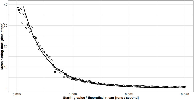
Figure 7. Mean hitting time of an Ornstein-Uhlenbeck process as a function of the starting value ${\mathrm{x}}_0$ (equal to its theoretical mean $\mathrm{\mu }$); the prediction of the analytical formula (line) and the results of the simulations (circles) are presented for a standard deviation of $\mathrm{\sigma }=0.010$ tons/second and a stiffness value of $\mathrm{\theta }=2$.

Figure 8 displays the comparison between the minimal models and the output simulations for the lagged recovery TISP model (lag $l=1$), in the case of an Ornstein-Uhlenbeck process and an uncorrelated Gaussian input. Both series coincide seamlessly for the uncorrelated input type. On the contrary, the discrepancies for the OU-process tend to increase along the x-axis which is confirmed by the Bland-Altman diagram (see Supplementary Material A: Figure A.6). The Authors exclude a systematic divergence between the minimal model and the output simulation, since the mean difference between them is close to zero regardless. The inherent random error presumably originates in the fact that for larger starting values/theoretical mean values (i.e., very short average hitting times/simulation lengths) an OU-process may spend a considerable period above or below the threshold and, therefore, the arithmetic mean of the simulated output is distorted by chance. Selecting a smaller simulation step would resolve this problem but is computationally very expensive.

Figure 8

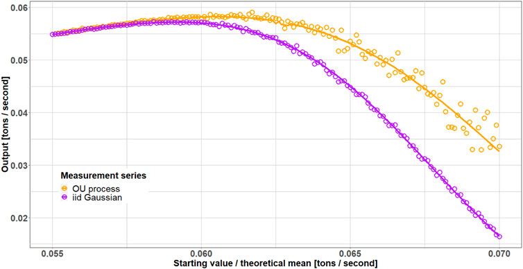
Figure 8. Output mass flow as a function of the starting value ${\mathrm{x}}_0$ (equal to its theoretical mean $\mathrm{\mu }$) for the uncorrelated Gaussian distribution (purple) and an Ornstein-Uhlenbeck process (orange); the results of the analytical model and the simulations are presented for standard deviation, stiffness and, lag values of $\mathrm{\sigma }=0.010$ tons/second, $\mathrm{\theta }=2$, and $\mathrm{l}=1$, respectively; for each probability model the results of the minimal models (continuous lines) and the simulations (circles) are presented.

Apart from this, Figure 8 also suggests that a production device powered by OU-noise input could be less susceptible to the disruptive threshold, as the curve associated with the uncorrelated Gaussian noise sinks much quicker. For a starting value/theoretical mean equal to the size of the disruptive threshold, the curves differ by already 50 percent. This is due to the mean-reverting behavior of the OU-process or the system operator that meticulously attempts to counterbalance performance fluctuations. Lastly, the authors monitored what consequences a change in the input distribution standard deviation or stiffness has on the location of the maximum performance. The position of the maximum appears to move logarithmically with the stiffness and inversely proportional with the standard deviation (see Supplementary Material A: Figure A.7). Thus, the larger the stiffness (or the more the input fluctuations are regulated by the system operator), the better the performance.

8 Conclusion

8.1 Summary

In this article, the authors have examined the output characteristics of several threshold-impeded stochastic production (TISP) systems using minimal models and simulations. The output experiments differ in terms of their input fluctuations (e.g., Gaussian or Weibull noise), application scenarios (i.e., steel continuous casting and wind turbines), and nonlinear features of the transformation (e.g., number of thresholds, magnitude of the penalties/lags). The influence of multiple input characteristics (e.g., noise distribution width) on the position of the maximum output performance in the parameter space has been explored. It turns out that for the continuous casting application scenario, neither the size of the penalty nor the duration of the lag have a significant effect on the maximum output, while they are essential for the calculation of the maximum power that can be generated by wind turbines. Ultimately, time-correlated and time-uncorrelated inputs have been compared by applying a simple nonlinear transformation to a mean-reversing Ornstein-Uhlenbeck process and uncorrelated Gaussian noise. The authors showed that a hypothetical production apparatus fuelled by OU-noise input would be superior to an equivalent apparatus fuelled by uncorrelated Gaussian noise (provided with the same system and noise parameters). Hence, a machine operator that constantly tries to dampen the input fluctuations of a TISP-type system improves the output performance.

8.2 Impact and practical relevance

Our work has further highlighted and developed the work of Merten et al. (2022b) as they essentially describe the existence of a TISP system in the continuous casting of steel (see Section 3). Clearly, in the case of a maximum possible steel flow around $0.070$ tons per second, the choice of the mean production level is immensely important because, for example, overshooting the optimal level by less than eight percent can theoretically lead to a production loss that is greater than 23 percent (see Figure 5 (a)). In fact, since the introduction of the novel production strategy at the steel factory investigated in Merten et al. (2022b) the ratio of devaluated casting products has gone down by more than 50 percent. If the value of devaluated products depreciated by just 20 percent on average and if one assumes a mean mass flow of 0.05 tons per second as well as a steel price of 1000 US dollars per ton, this decrease (5.5 percent to roughly 2.7 percent) in downgrading percentage would entail an optimization potential of almost 9 million US dollars per year. Analogously, selecting a suitable location and thereby the right wind speed pattern is crucial for the construction of new wind farms (see Figure 6). In a way, the authors have extended the approach of Salameh and Safari (1992) who developed a framework to determine the correct wind turbine parameters for a specific wind site by including additional degrees of freedom related to the amount of energy necessary to restart a wind turbine after it has been shut down as well as the length of its idle time following a threshold violation.

8.3 Future outlook

With this work the authors want to draw attention to production situations, where a balance is required between the process stability and the strive for increased production–due to both input stochasticity and the presence of disruptive thresholds. Often such a balance is hidden within the intricacies of the production process (e.g., disruptive thresholds masked as load-dependent errors or sudden declines in product quality when reaching critical load levels in the production system). Identification of such situations requires a dialog between different divisions of a production facility that are responsible for maximizing production (e.g., operations management) or surveying the occurrence of component failures and errors, as well as quality standards (e.g., quality control). The authors believe that the procedure can contribute to this dialog as it is applicable to any production system that a) relies on stochastic inputs and b) is subject to nonlinear transformations involving disruptive thresholds. Accordingly, the authors would like to encourage researchers to test this methodology with regards to a wider range of applications scenarios and extra technical details such as different noise correlations and flavors. One potential scenario for this endeavour is portrayed by a situation where a company wants to sell a product through its website. Obviously, more website visitors should lead to greater sales; however, once a critical number of visitors is reached the website server might crash resulting in extended downtimes. The respective company should adjust its marketing activities to account for this possibility.

In earlier publications (Merten et al., 2022a; Merten et al., 2022b) we have studied the technical details and algorithmic challenges of steel production in some detail. Hence, the description here has a stronger emphasis on this example. With our second example, wind farms, we wish to emphasize that the TISP systems are not just confined to this one application domain. We hope that other researchers are encouraged to think about their production systems from a TISP perspective.

Data availability statement

The raw data supporting the conclusion of this article will be made available by the authors, without undue reservation.

Author contributions

DM: Conceptualization, Data curation, Formal Analysis, Investigation, Methodology, Software, Validation, Visualization, Writing–original draft, Writing–review and editing. AL: Conceptualization, Formal Analysis, Investigation, Methodology, Supervision, Validation, Writing–review and editing. YU: Funding acquisition, Project administration, Resources, Supervision, Writing–review and editing. M-TH: Conceptualization, Funding acquisition, Methodology, Project administration, Resources, Supervision, Validation, Writing–review and editing.

Funding

The author(s) declare that no financial support was received for the research, authorship, and/or publication of this article.

Conflict of interest

Author DM was employed by Accenture GmbH at the time of submission.

The remaining authors declare that the research was conducted in the absence of any commercial or financial relationships that could be construed as a potential conflict of interest.

Publisher’s note

All claims expressed in this article are solely those of the authors and do not necessarily represent those of their affiliated organizations, or those of the publisher, the editors and the reviewers. Any product that may be evaluated in this article, or claim that may be made by its manufacturer, is not guaranteed or endorsed by the publisher.

Supplementary material

The Supplementary Material for this article can be found online at: https://www.frontiersin.org/articles/10.3389/fieng.2024.1353531/full#supplementary-material

References

Alili, L. P., Patie, P., and Pedersen, J. L. (2005). Representations of the first hitting time density of an Ornstein-Uhlenbeck process. Stoch. Models 21 (4), 967–980. doi:10.1080/15326340500294702

CrossRef Full Text | Google Scholar

Alkan, B., Vera, D. A., Ahmad, M., Ahmad, B., and Harrison, R. (2018). Complexity in manufacturing systems and its measures: a literature review. Eur. J. Industrial Eng. 12 (1), 116–150. doi:10.1504/ejie.2018.089883

CrossRef Full Text | Google Scholar

Angkiriwang, R., Pujawan, I. N., and Santosa, B. (2014). Managing uncertainty through supply chain flexibility: reactive vs. proactive approaches. Prod. Manuf. Res. 2 (1), 50–70. doi:10.1080/21693277.2014.882804

CrossRef Full Text | Google Scholar

Aouam, T., Geryl, K., Kumar, K., and Brahimi, N. (2018). Production planning with order acceptance and demand uncertainty. Comput. Operations Res. 91, 145–159. doi:10.1016/j.cor.2017.11.013

CrossRef Full Text | Google Scholar

Archer, C. L., and Jacobson, M. Z. (2007). Supplying baseload power and reducing transmission requirements by interconnecting wind farms. J. Appl. meteorology Climatol. 46 (11), 1701–1717. doi:10.1175/2007jamc1538.1

CrossRef Full Text | Google Scholar

Arinez, J. F., Chang, Q., Gao, R. X., Xu, C., and Zhang, J. (2020). Artificial intelligence in advanced manufacturing: current status and future outlook. J. Manuf. Sci. Eng. 142 (11), 110804. doi:10.1115/1.4047855

CrossRef Full Text | Google Scholar

Batterman, R. W., and Rice, C. C. (2014). Minimal model explanations. Philosophy Sci. 81 (3), 349–376. doi:10.1086/676677

CrossRef Full Text | Google Scholar

Bendat, J. S., and Piersol, A. G. (2011). Random data: analysis and measurement procedures. New Jersey, United States: John Wiley and Sons.

Google Scholar

Bergey, K. H. (1979). The Lanchester-Betz limit (energy conversion efficiency factor for windmills). J. Energy 3 (6), 382–384. doi:10.2514/3.48013

CrossRef Full Text | Google Scholar

Bertsimas, D., and Thiele, A. (2014). “Robust and data-driven optimization: modern decision making under uncertainty,” in Models, methods, and applications for innovative decision making. Editor P. Grey (Catonsville, MD, United States: INFORMS), 95–122.

CrossRef Full Text | Google Scholar

Carrillo, C., Obando Montaño, A., Cidrás, J., and Díaz-Dorado, E. (2013). Review of power curve modelling for wind turbines. Renew. Sustain. Energy Rev. 21, 572–581. doi:10.1016/j.rser.2013.01.012

CrossRef Full Text | Google Scholar

Cassola, F., Burlando, M., Antonelli, M., and Ratto, C. F. (2008). Optimization of the regional spatial distribution of wind power plants to minimize the variability of wind energy input into power supply systems. J. Appl. Meteorology Climatol. 47 (12), 3099–3116. doi:10.1175/2008jamc1886.1

CrossRef Full Text | Google Scholar

Castellani, F., Astolfi, D., Garinei, A., Proietti, S., Sdringola, P., Terzi, L., et al. (2015). How wind turbines alignment to wind direction affects efficiency? A case study through SCADA data mining. Energy Procedia 75, 697–703. doi:10.1016/j.egypro.2015.07.495

CrossRef Full Text | Google Scholar

Cerbone, G., Ricciardi, L. M., and Sacerdote, L. (1981). Mean variance and skewness of the first passage time for the Ornstein-Uhlenbeck process. Cybern. Syst. 12 (4), 395–429. doi:10.1080/01969728108927683

CrossRef Full Text | Google Scholar

Chankov, S., Hütt, M. T., and Bendul, J. (2016). Synchronization in manufacturing systems: quantification and relation to logistics performance. Int. J. Prod. Res. 54 (20), 6033–6051. doi:10.1080/00207543.2016.1165876

CrossRef Full Text | Google Scholar

Chankov, S., Hütt, M. T., and Bendul, J. (2018). Influencing factors of synchronization in manufacturing systems. Int. J. Prod. Res. 56 (14), 4781–4801. doi:10.1080/00207543.2017.1400707

CrossRef Full Text | Google Scholar

Chatterjee, J., and Dethlefs, N. (2021). Scientometric review of artificial intelligence for operations and maintenance of wind turbines: the past, present and future. Renew. Sustain. Energy Rev. 144, 111051. doi:10.1016/j.rser.2021.111051

CrossRef Full Text | Google Scholar

Cho, S., and Erkoc, M. (2009). Design of predictable production scheduling model using control theoretic approach. Int. J. Prod. Res. 47 (11), 2975–2993. doi:10.1080/00207540701749281

CrossRef Full Text | Google Scholar

Correa, H. L. (1992). The links between uncertainty, variability of outputs and flexibility in manufacturing systems. Coventry, England: University of Warwick. Doctoral dissertation.

Google Scholar

Cowling, P. I., Ouelhadj, D., and Petrovic, S. (2003). A multi-agent architecture for dynamic scheduling of steel hot rolling. J. intelligent Manuf. 14, 457–470. doi:10.1023/a:1025701325275

CrossRef Full Text | Google Scholar

Cowling, P. I., Ouelhadj, D., and Petrovic, S. (2004). Dynamic scheduling of steel casting and milling using multi-agents. Prod. Plan. Control 15 (2), 178–188. doi:10.1080/09537280410001662466

CrossRef Full Text | Google Scholar

Dotoli, M., Fay, A. M., Miśkowicz, M., and Seatzu, C. (2019). An overview of current technologies and emerging trends in factory automation. Int. J. Prod. Res. 57, 5047–5067. doi:10.1080/00207543.2018.1510558

CrossRef Full Text | Google Scholar

Ettlie, J. E. (1990). What makes a manufacturing firm innovative? Acad. Manag. Perspect. 4 (4), 7–20. doi:10.5465/ame.1990.4277195

CrossRef Full Text | Google Scholar

Feng, J., and Shen, W. Z. (2017). Wind farm power production in the changing wind: robustness quantification and layout optimization. Energy Convers. Manag. 148, 905–914. doi:10.1016/j.enconman.2017.06.005

CrossRef Full Text | Google Scholar

Gerwin, D., and Tarondeau, J. C. (1982). Case studies of computer integrated manufacturing systems: a view of uncertainty and innovation processes. J. Operations Manag. 2 (2), 87–99. doi:10.1016/0272-6963(82)90025-0

CrossRef Full Text | Google Scholar

Ghobakhloo, M. (2020). Industry 4.0, digitization, and opportunities for sustainability. J. Clean. Prod. 252, 119869. doi:10.1016/j.jclepro.2019.119869

CrossRef Full Text | Google Scholar

Gillespie, D. T. (1996). Exact numerical simulation of the Ornstein-Uhlenbeck process and its integral. Phys. Rev. E 54 (2), 2084–2091. doi:10.1103/physreve.54.2084

PubMed Abstract | CrossRef Full Text | Google Scholar

Groover, M. P. (2006). Fundamentals of modern manufacturing: materials, processes, and systems. New Jersey, United States: John Wiley and Sons.

Google Scholar

Guo, Q., and Tang, L. (2019). Modelling and discrete differential evolution algorithm for order rescheduling problem in steel industry. Comput. Industrial Eng. 130, 586–596. doi:10.1016/j.cie.2019.03.011

CrossRef Full Text | Google Scholar

Gupta, D., and Maravelias, C. T. (2020). Framework for studying online production scheduling under endogenous uncertainty. Comput. Chem. Eng. 135, 106670. doi:10.1016/j.compchemeng.2019.106670

CrossRef Full Text | Google Scholar

Hau, E. (2013). Wind turbines: fundamentals, technologies, application, economics. Springer Science and Business Media.

Google Scholar

Iglesias-Escudero, M., Villanueva-Balsera, J., Ortega-Fernandez, F., and Rodriguez-Montequín, V. (2019). Planning and scheduling with uncertainty in the steel sector: a review. Appl. Sci. 9 (13), 2692. doi:10.3390/app9132692

CrossRef Full Text | Google Scholar

Irving, W. R. (1993). Continuous casting of steel. UK: The Institute of Materials.

Google Scholar

Jamalnia, A., Yang, J. B., Feili, A., Xu, D. L., and Jamali, G. (2019). Aggregate production planning under uncertainty: a comprehensive literature survey and future research directions. Int. J. Adv. Manuf. Technol. 102 (1), 159–181. doi:10.1007/s00170-018-3151-y

CrossRef Full Text | Google Scholar

Jeon, S. M., and Kim, G. (2016). A survey of simulation modeling techniques in production planning and control (PPC). Prod. Plan. Control 27 (5), 360–377. doi:10.1080/09537287.2015.1128010

CrossRef Full Text | Google Scholar

Katzenstein, W., Fertig, E., and Apt, J. (2010). The variability of interconnected wind plants. Energy policy 38 (8), 4400–4410. doi:10.1016/j.enpol.2010.03.069

CrossRef Full Text | Google Scholar

Klimstra, J., and Hotakainen, M. (2011). Smart power generation.

Google Scholar

Koh, S. C., and Saad, S. M. (2002). Development of a business model for diagnosing uncertainty in ERP environments. Int. J. Prod. Res. 40 (13), 3015–3039. doi:10.1080/00207540210140077

CrossRef Full Text | Google Scholar

Koh, S. C., Saad, S. M., and Jones, M. H. (2002). Uncertainty under MRP-planned manufacture: review and categorization. Int. J. Prod. Res. 40 (10), 2399–2421. doi:10.1080/00207540210136487

CrossRef Full Text | Google Scholar

Kwon, S. D. (2010). Uncertainty analysis of wind energy potential assessment. Appl. Energy 87 (3), 856–865. doi:10.1016/j.apenergy.2009.08.038

CrossRef Full Text | Google Scholar

Laing, C., and Lord, G. J. (2010). Stochastic methods in neuroscience. Oxford, United Kingdom: Oxford University Press.

Google Scholar

Lee, J., Lapira, E., Bagheri, B., and Kao, H. A. (2013). Recent advances and trends in predictive manufacturing systems in big data environment. Manuf. Lett. 1 (1), 38–41. doi:10.1016/j.mfglet.2013.09.005

CrossRef Full Text | Google Scholar

Li, C., and Thomas, B. G. (2000). “Analysis of the potential productivity of continuous cast molds,” in The Brimacombe Memorial Symposium, Vancouver, October 1-4, 2000, 595–611.

Google Scholar

Li, Y., Carabelli, S., Fadda, E., Manerba, D., Tadei, R., and Terzo, O. (2020). Machine learning and optimization for production rescheduling in Industry 4.0. Int. J. Adv. Manuf. Technol. 110, 2445–2463. doi:10.1007/s00170-020-05850-5

CrossRef Full Text | Google Scholar

Lin, J., and Naim, M. M. (2019). Why do nonlinearities matter? The repercussions of linear assumptions on the dynamic behaviour of assemble-to-order systems. Int. J. Prod. Res. 57 (20), 6424–6451. doi:10.1080/00207543.2019.1566669

CrossRef Full Text | Google Scholar

Liu, H., Shi, J., and Qu, X. (2013). Empirical investigation on using wind speed volatility to estimate the operation probability and power output of wind turbines. Energy Convers. Manag. 67, 8–17. doi:10.1016/j.enconman.2012.10.016

CrossRef Full Text | Google Scholar

Louhenkilpi, S. (2014). “Chapter 1.8 - continuous casting of steel,” in Treatise on process metallurgy. Editor S. Seetharaman (Amsterdam, Netherlands: Elsevier), 373–434.

CrossRef Full Text | Google Scholar

Maller, R. A., Müller, G., and Szimayer, A. (2009). “Ornstein–Uhlenbeck processes and extensions,” in Handbook of financial time series. Editors T. G. Andersen, R. A. Davis, J. P. Kreiß, and T. V. Mikosch (Cham: Springer Science and Business Media), 421–437.

CrossRef Full Text | Google Scholar

Manwell, J. F., McGowan, J. G., and Rogers, A. L. (2010). Wind energy explained: theory, design and application. New Jersey, United States: John Wiley and Sons.

Google Scholar

Martin Bland, J., and Altman, D. (1986). Statistical methods for assessing agreement between two methods of clinical measurement. Lancet 327 (8476), 307–310. doi:10.1016/s0140-6736(86)90837-8

PubMed Abstract | CrossRef Full Text | Google Scholar

Merten, D., Hütt, M., Uygun, Y., Özgür, A., and Klein, C. (2024). “Comparative study of two genetic algorithms for steel production planning under different order,” in Steel 4.0: digitalization in steel industry. Editors Y. Uygun, A. Özgür, and M. Hütt (Cham: Springer Nature).

Google Scholar

Merten, D., Hütt, M.-T., and Uygun, Y. (2022a). A network analysis of decision strategies of human experts in steel production. Submitt. Comput. Industrial Eng. doi:10.1016/j.cie.2022.108120

CrossRef Full Text | Google Scholar

Merten, D., Hütt, M.-T., and Uygun, Y. (2022b). The effect of the slab width on the choice of the appropriate casting. J. Iron Steel Res. Int., 71–79. doi:10.1007/s42243-021-00729-5

CrossRef Full Text | Google Scholar

Morgan, E. C., Lackner, M., Vogel, R. M., and Baise, L. G. (2011). Probability distributions for offshore wind speeds. Energy Convers. Manag. 52 (1), 15–26. doi:10.1016/j.enconman.2010.06.015

CrossRef Full Text | Google Scholar

Mourtzis, D. (2020). Simulation in the design and operation of manufacturing systems: state of the art and new trends. Int. J. Prod. Res. 58 (7), 1927–1949. doi:10.1080/00207543.2019.1636321

CrossRef Full Text | Google Scholar

Mourtzis, D., Doukas, M., and Bernidaki, D. (2014). Simulation in manufacturing: review and challenges. Procedia Cirp 25, 213–229. doi:10.1016/j.procir.2014.10.032

CrossRef Full Text | Google Scholar

Negahban, A., and Smith, J. S. (2014). Simulation for manufacturing system design and operation: literature review and analysis. J. Manuf. Syst. 33 (2), 241–261. doi:10.1016/j.jmsy.2013.12.007

CrossRef Full Text | Google Scholar

Ouelhadj, D., Petrovic, S., Cowling, P. I., and Meisels, A. (2004). Inter-agent cooperation and communication for agent-based robust dynamic scheduling in steel production. Adv. Eng. Inf. 18 (3), 161–172. doi:10.1016/j.aei.2004.10.003

CrossRef Full Text | Google Scholar

Özgür, A., Uygun, Y., and Hütt, M.-T. (2021). A review of planning and scheduling methods for hot rolling mills in steel production. Comput. Industrial Eng. 151, 106606. doi:10.1016/j.cie.2020.106606

CrossRef Full Text | Google Scholar

Oztemel, E., and Gursev, S. (2020). Literature review of Industry 4.0 and related technologies. J. Intelligent Manuf. 31 (1), 127–182. doi:10.1007/s10845-018-1433-8

CrossRef Full Text | Google Scholar

Peidro, D., Mula, J., Poler, R., and Lario, F. C. (2009). Quantitative models for supply chain planning under uncertainty: a review. Int. J. Adv. Manuf. Technol. 43 (3-4), 400–420. doi:10.1007/s00170-008-1715-y

CrossRef Full Text | Google Scholar

Pervozvanskii, A. A. (1965). “Random processes,” in Nonlinear control systems. Editor A. A. Pervozvanskii (New Jersey, United States: Elsevier).

Google Scholar

Psarommatis, F., Martiriggiano, G., Zheng, X., and Kiritsis, D. (2021). A generic methodology for calculating rescheduling time for multiple unexpected events in the era of zero defect manufacturing. Front. Mech. Eng. 7, 646507. doi:10.3389/fmech.2021.646507

CrossRef Full Text | Google Scholar

Ricciardi, L. M., and Sacerdote, L. (1979). The Ornstein-Uhlenbeck process as a model for neuronal activity. Biol. Cybern. 35 (1), 1–9. doi:10.1007/bf01845839

PubMed Abstract | CrossRef Full Text | Google Scholar

Ritter, M., and Deckert, L. (2017). Site assessment, turbine selection, and local feed-in tariffs through the wind energy index. Appl. energy 185, 1087–1099. doi:10.1016/j.apenergy.2015.11.081

CrossRef Full Text | Google Scholar

Roy *, R., Adesola, B. A., and Thornton, S. (2004). Development of a knowledge model for managing schedule disturbance in steel-making. Int. J. Prod. Res. 42 (18), 3975–3994. doi:10.1080/00207540410001716453

CrossRef Full Text | Google Scholar

Salameh, Z. M., and Safari, I. (1992). Optimum windmill-site matching. IEEE Trans. Energy Convers. 7 (4), 669–676. doi:10.1109/60.182649

CrossRef Full Text | Google Scholar

Santos, C. A., Spim, J. A., and Garcia, A. (2003). Mathematical modeling and optimization strategies (genetic algorithm and knowledge base) applied to the continuous casting of steel. Eng. Appl. Artif. Intell. 16 (5-6), 511–527. doi:10.1016/s0952-1976(03)00072-1

CrossRef Full Text | Google Scholar

Sreedevi, R., and Saranga, H. (2017). Uncertainty and supply chain risk: the moderating role of supply chain flexibility in risk mitigation. Int. J. Prod. Econ. 193, 332–342. doi:10.1016/j.ijpe.2017.07.024

CrossRef Full Text | Google Scholar

Stevens, M. J., and Smulders, P. T. (1979). The estimation of the parameters of the Weibull wind speed distribution for wind energy utilization purposes. Wind Eng., 132–145.

Google Scholar

Thomas, B. G. (2002). Modeling of the continuous casting of steel—past, present, and future. Metallurgical Mater. Trans. B 33 (6), 795–812. doi:10.1007/s11663-002-0063-9

CrossRef Full Text | Google Scholar

Thomas, M. (1975). Some mean first-passage time approximations for the Ornstein-Uhlenbeck process. J. Appl. Probab. 12 (3), 600–604. doi:10.1017/s0021900200048439

CrossRef Full Text | Google Scholar

Tordecilla, R. D., Juan, A. A., Montoya-Torres, J. R., Quintero-Araujo, C. L., and Panadero, J. (2021). Simulation-optimization methods for designing and assessing resilient supply chain networks under uncertainty scenarios: a review. Simul. Model. Pract. theory 106, 102166. doi:10.1016/j.simpat.2020.102166

PubMed Abstract | CrossRef Full Text | Google Scholar

Uhlenbeck, G. E., and Ornstein, L. S. (1930). On the theory of the Brownian motion. Phys. Rev. 36 (5), 823–841. doi:10.1103/physrev.36.823

CrossRef Full Text | Google Scholar

Vasicek, O. (1977). An equilibrium characterization of the term structure. J. Financial Econ. 5 (2), 177–188. doi:10.1016/0304-405x(77)90016-2

CrossRef Full Text | Google Scholar

Vieira, G. E., Herrmann, J. W., and Lin, E. (2003). Rescheduling manufacturing systems: a framework of strategies, policies, and methods. J. Sched. 6, 39–62. doi:10.1023/a:1022235519958

CrossRef Full Text | Google Scholar

Wang, Y., and Zhang, L. (2010). Transient fluid flow phenomena during continuous casting: Part II—cast speed change, temperature fluctuation, and steel grade mixing. ISIJ Int. 50 (12), 1783–1791. doi:10.2355/isijinternational.50.1783

CrossRef Full Text | Google Scholar

Wood, A. J., Wollenberg, B. F., and Sheblé, G. B. (2013). Power generation, operation, and control. New Jersey, United States: John Wiley and Sons.

Google Scholar

Xu, L. D., Xu, E. L., and Li, L. (2018). Industry 4.0: state of the art and future trends. Int. J. Prod. Res. 56 (8), 2941–2962. doi:10.1080/00207543.2018.1444806

CrossRef Full Text | Google Scholar

Yan, Y. (2015). “Nacelle orientation based health indicator for wind turbines,” in IEEE Conference on Prognostics and Health Management (PHM), Austin, TX, USA, June 22-25, 2015 (IEEE), 1–7.

CrossRef Full Text | Google Scholar

Zhang, L., Zhou, L., Ren, L., and Laili, Y. (2019). Modeling and simulation in intelligent manufacturing. Comput. Industry 112, 103123. doi:10.1016/j.compind.2019.08.004

CrossRef Full Text | Google Scholar

Zhang, Q., Wang, L., and Wang, X. (2006). Influence of casting speed variation during unsteady continuous casting on non-metallic inclusions in IF steel slabs. ISIJ Int. 46 (10), 1421–1426. doi:10.2355/isijinternational.46.1421

CrossRef Full Text | Google Scholar

Zhang, Q., and Wang, X. (2010). Numerical simulation of influence of casting speed variation on surface fluctuation of molten steel in mold. J. Iron Steel Res. Int. 17 (8), 15–19. doi:10.1016/s1006-706x(10)60121-5

CrossRef Full Text | Google Scholar

Zhong, L., Li, B., Zhu, Y., Wang, R., Wang, W., and Zhang, X. (2007). Fluid flow in a four-strand bloom continuous casting tundish with different flow modifiers. ISIJ Int. 47 (1), 88–94. doi:10.2355/isijinternational.47.88

CrossRef Full Text | Google Scholar

Zhong, R. Y., Xu, X., Klotz, E., and Newman, S. T. (2017). Intelligent manufacturing in the context of industry 4.0: a review. Engineering 3 (5), 616–630. doi:10.1016/j.eng.2017.05.015

CrossRef Full Text | Google Scholar