 Max Riekeles
 Hadi Albalkhi
 Megan Marie Dubay
 Jay Nadeau
 Christian A. Lindensmith
94% of researchers rate our articles as excellent or good
Learn more about the work of our research integrity team to safeguard the quality of each article we publish.
Find out more
METHODS article
Front. Imaging, 10 May 2024
Sec. Image Coding and Security
Volume 3 - 2024 | https://doi.org/10.3389/fimag.2024.1393314
This article is part of the Research TopicHorizons in ImagingView all 6 articles
Quantitative tracking of rapidly moving micron-scale objects remains an elusive challenge in microscopy due to low signal-to-noise. This paper describes a novel method for tracking micron-sized motile organisms in off-axis Digital Holographic Microscope (DHM) raw holograms and/or reconstructions. We begin by processing the microscopic images with the previously reported Holographic Examination for Life-like Motility (HELM) software, which provides a variety of tracking outputs including motion history images (MHIs). MHIs are stills of videos where the frame-to-frame changes are indicated with color time-coding. This exposes tracks of objects that are difficult to identify in individual frames at a low signal-to-noise ratio. The visible tracks in the MHIs are superior to tracks identified by all tested automated tracking algorithms that start from object identification at the frame level, particularly in low signal-to-noise ratio data, but do not provide quantitative track data. In contrast to other tracking methods, like Kalman filter, where the recording is analyzed frame by frame, MHIs show the whole time span of particle movement at once and eliminate the need to identify objects in individual frames. This feature also enables post-tracking identification of low-SNR objects. We use these tracks, rather than object identification in individual frames, as a basis for quantitative tracking of Bacillus subtilis by first generating MHIs from X, Y, and t stacks (raw holograms or a projection over reconstructed planes), then using a region-tracking algorithm to identify and separate swimming pathways. Subsequently, we identify each object's Z plane of best focus at the corresponding X, Y, and t points, yielding ap full description of the swimming pathways in three spatial dimensions plus time. This approach offers an alternative to object-based tracking for processing large, low signal-to-noise datasets containing highly motile organisms.
The importance of bacterial motility tracking has been appreciated since at least the 1970s, with the pioneering work of the late Howard Berg (Berg, 1971; Berg and Brown, 1972, 1974; Berg and Anderson, 1973). Manual tracking of a few cells at a time has enabled quantitative characterization of swimming patterns seen in different strains, such as run and tumble, run-reverse-flick, run and slow, stop and coil, and push and pull, which has allowed for elucidation of the underlying physics and biology of locomotion at low Reynolds number. Recent advances in microscopic spatial and temporal resolution have revealed surprising features even in these simple behaviors, such as the role of cell body shape in swimming and correlations of flagellar motion with tumbles (Liu et al., 2014; Turner et al., 2016; Schuech et al., 2019). The advances in microscopy that have enabled these studies have made it possible to collect large amounts of data, but processing of the data remains difficult and time consuming, particularly for bacteria near the resolution limit of the instruments. For some applications, such as remote field instruments and planetary space missions, some degree of autonomous tracking is desirable in order to reduce the amount of data that needs to be sent over limited data links (Wronkiewicz and Lee, 2021; Wronkiewicz et al., 2024). We present here an approach designed to be as independent of prior sample knowledge as possible, while also being computationally low-cost. This methodology is not only suitable for fast processing of microbial motility datasets, but makes it particularly well-suited for in-situ measurements in contexts where computing power and data transmission volume may be limited.
A tremendous amount of work still remains to be done in this field, because quantification of bacterial swimming motility in 3D is challenging, presenting difficulties of data acquisition and analysis that are not seen with other particle tracking situations such as Brownian motion. Bacteria can swim tens or even hundreds of cell lengths per second in X, Y, and Z, leave and re-enter the microscopic field of view, and change directions abruptly and rapidly. In any but the sparsest cultures, tracks of multiple cells will overlap. Tracking is usually performed by identifying objects in individual frames and then linking tracks based on object locations from frame to frame. Even if all objects are identified correctly at each time point, linking is error-prone. Computational tracking algorithms usually use a cost (or energy) function that assumes some aspects of the velocity such as the trajectory smoothness or maximum acceleration; examples are the Linear Assignment (LAP) tracker and Kalman filter (Jaqaman et al., 2008; Li et al., 2010). However, these velocity parameters are difficult to define in most cases, especially in heterogeneous populations or with unknown organisms because many microbes are capable of abrupt changes in velocity. In a LAP tracker, objects are first identified in individual frames, followed by frame-to-frame assignment of particles to track segments, and stitching of segments into full tracks. Such trackers depend heavily on the ability to reliably identify candidate objects in individual frames without the ability to take advantage of the past or future locations of the objects. Manual breaking and stitching of tracks is necessary after any automated tracking procedure and can be as time- and labor-intensive as full manual tracking.
Tracking is made even more difficult when particle recognition is poor, which is true for all light microscopy techniques, including phase contrast and digital holographic microscopy (DHM) unless the particles are highly light absorbing. The advantage of DHM is that it is a volumetric technique where a single XY snapshot (the hologram) may be digitally refocused through a chosen Z depth with an appropriate Z-slice spacing based upon the axial resolution of the instrument (Kim, 2010; Yu et al., 2014). Resolution remains optimal through approximately 100 times the depth of field obtained with comparable resolution ordinary brightfield microscopy. DHM with automated tracking has shown great success for the analysis of swimming eukaryotes >10 μm in diameter (Sheng et al., 2007; Tang et al., 2022); however, tracking of prokaryotes is substantially more difficult because the objects to be tracked are close to the resolution limit. Results have been reported from various groups (Wilson and Zhang, 2012; Molaei et al., 2014; Cheong et al., 2015; Wang et al., 2016; Farthing et al., 2017; Kühn et al., 2018), but requires often time-consuming processing and de-noising and/or manual tracking (Dubay et al., 2022a).
We recently presented tracking results for DHM recordings of cultures of Bacillus subtilis swimming at different temperatures, achieved using the LAP tracker (Dubay et al., 2022b). To obtain the tracks, the holograms were reconstructed into Z stacks, then a maximum projection was taken through the Z stack to yield a higher signal-to-noise X,Y time series. These were then tracked using an open source software package developed by our team called Holographic Examination for Life-like Motility (HELM) (Wronkiewicz and Lee, 2021; Wronkiewicz et al., 2024). HELM offers color-coded Motion History Images (MHI) in addition to automated tracking based on the LAP algorithm. An MHI is a two-dimensional image made from a time series, where at each pixel the maximum intensity change over a timespan is represented. The color of each pixel relates to the specific time in which its intensity change was maximal. In contrast to the LAP tracker, where the recording is analyzed frame by frame, the MHIs show the whole time span of particle movement at once and eliminate the need to identify objects within individual frames. The streaks and paths are a simple, human-interpretable way of representing swimming microbes that effectively increase the signal to noise ratio. In all of our data, the MHI indicated full, continuous tracks of individual swimming cells that were poorly captured by the LAP tracker. An overlaid video allows the user to confirm that a track corresponds to the motion of a single cell.
In this work, we begin with the MHI output of selected datasets and use them as a tool to extract X, Y, Z, and t coordinates of swimming microorganisms. Our approach is a quantitative extension of a commonly used approach of color-coded display of image-to-image changes (Thornton et al., 2020; Wronkiewicz and Lee, 2021). The novelty of our approach is to identify candidate objects and their locations first by their tracks and then go back to find the objects within individual frames, rather than identifying objects in frames and stitching tracks together.
We use data sets recorded by an off-axis digital holographic microscope described in Wallace et al. (2015). Briefly, a single-mode laser (wavelengths used are usually 405 or 520 nm) is collimated and passed through separate reference and sample channels held in a single plane to prevent misalignment. The objective lenses are simple achromats (numerical aperture 0.31), yielding an effective magnification of ~20 × and XY spatial resolution of ~1.0 μm. Since focusing is performed numerically with DHM, the sample stage is fixed in position with the in-focus plane Z = 0 at approximately the center of the sample chamber. The camera is a Prosilica 2460GT (Allied Vision, purchased from Edmund Optics) monochrome camera with 4.20 MPixel resolution and 15 frames/s maximum frame rate. The images had a field of view of 365 μm × 365 μm and were saved as 2,048 px × 2,048 px (see Supplementary material for a schematic overview).
The first dataset used here (DS1) was reported in our previous work and the raw data are publicly available on Dryad (Johnston et al., 2022). The test data represent B. subtilis type strain (ATCC 6051) at a concentration of approximately 107/mL in a sample chamber 1.0 mm in depth, freely swimming in culture medium at 28°C. The dataset consists of 851 time points (56 seconds). Additionally, we compare our tracking results with hand-tracked tracks of two other B. subtilis data sets from the JPL Open Repository (DS2, DS3) (Wronkiewicz et al., 2022). An additional dataset representing the microalga Chlamydomonas (Carolina Biological Supply Item # 152030) is also included from this repository (DS4) (see Supplementary material for overview).
In our processing, two versions of MHIs are created for comparison (Figure 1): (a) MHIs directly from the median-subtracted holograms, and (b) MHIs from maximum-Z projections of the amplitude reconstructions of the holograms. For data taken with a shallow depth of field, the simple MHIs may be sufficiently high SNR that the extra computational cost of volume reconstruction and z-projection is not necessary. For deep fields where many objects may be out of focus to varying degrees, the reconstruction and Z-projection brings all the objects to the same focus for xy tracking. To create these projections, the holograms are median subtracted before reconstruction, and then reconstructed every 4 μm for a defined Z range using the angular spectrum method implemented in a Fiji (Schindelin et al., 2012) plug-in (Cohoe et al., 2019). This hyperstack is then maximum projected through Z to create an X, Y, t series. The reconstructed holograms over multiple time points show occasional flashing, i.e., strong irregularities in illumination, probably caused by errors in the illumination or point vibration during the observation, which can lead to phase variation in the wavefront. To reduce this effect, the reconstructed images are equalized using the Histogram Matching Fiji plug-in (Burri, 2018). The purpose of this processing is to bring all objects into focus in a single plane via the reconstruction and projection, and normalization of the frame-to-frame brightness. This improves the signal to noise for the detection of objects that are far from focus in the raw holograms.
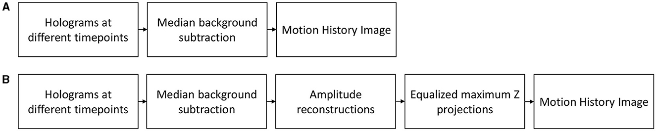
Figure 1. Workflow of Motion History Image generation. (A) The MHIs are created directly out of the holograms, (B) the MHIs are created out of the maximum-Z projections of the holograms. Background subtraction is performed in both generations.
The workflow of our software currently involves a human operator (Figure 2), but is amenable to automation, particularly for closely related data sets where the set of tuning parameters will be consistent across data sets. First, all the max-Z projections are examined and all “blobs” in the max-Z projection at all time points are detected in order to use them as seed points for finding tracks later. A blob is a group of pixels that contains the maximum-Z projected XY area of a candidate microbe or trackable object. Second, a region-growing algorithm is applied to the MHIs to obtain XY-coordinate sets of single tracks. In the rest of the paper, we will refer to a region that has been found as a track by the region-growing algorithm simply as a “track region.” In the next step, all the detected blobs are compared with a track region. Blobs that lay within a track region are used as the input for the Z-layer selection, which crops all Z-layers in a small track region around the blobs at a given time point and selects the Z-layers with the brightest and sharpest crops. The outputs for each particle are the XYZ coordinates, the timepoint t, and the size of the associated blob in the max-Z projections. The tracks are filtered by time, and DBSCAN is used in 3D to cluster and separate different tracks that lay within the XY coordinates of a track region.

Figure 2. Workflow of our semi-automated tracking software.
For blob detection, we use the SimpleBlobDetector class in the OpenCV library. The color filter and area filter is adjusted for optimum blob detection in a max-Z projection at a chosen time point. The time point, XY-coordinates of the blob center, and the size (diameter) of the detected blobs are saved.
Region-growing is a pixel-based image segmentation method. The goal of image segmentation techniques is to define different regions in an image. There are multiple approaches for image segmentation (for example, thresholding, where boundaries between regions are determined based on abrupt changes in grayscale intensity or color). The advantage of the region-growing algorithm lies in its simplicity. Its main assumption is that the neighboring pixels within one region have similar values. In the first step, the starting point or so-called seed point from which the track region can grow is set. The region-growing algorithm additionally requires that the points in a track region be connected in a defined way. If a neighbor pixel (meaning a pixel within a defined area around the seed point) has a value similar to the seed point, it is assigned to that track region, i.e., to that microbial path. Then the neighbor pixel is processed recursively. In contrast to traditional approaches using the region-growing algorithm, where the color (or greyscale) are the determining factors deciding if one pixel is to be assigned to the neighboring pixel, we use the values generated by the HELM software, which saves the timepoint at which the intensity change of each pixel was maximal. We have implemented two versions, which are identical except for the selection of the seed points:
• In the first version, the user sets the seed point by clicking on a location of the MHI (and therefore using color information). The user also sets the radius, which determined how many pixels around the center pixel should be taken into consideration, and the threshold, which indicated the allowed difference between center and neighbor pixels. Additionally, a rejection threshold is used to define how many neighboring pixels could have rejected a pixel without it being seen again by another neighboring pixel. For example, if the Rejection Threshold is 5, it means that a pixel could be rejected 5 times by a surrounding pixel; after that, it would be ignored and could not become part of the path again.
• In the second implementation, the seeds are selected automatically. For this, blobs are detected in the maximum-Z projection over all time points (see Section 3.2). To prevent redundancy, after a track is found, all blobs that lay on this track are removed and thus no longer considered as putative further seed points. A path is then saved if it exceeds a minimum size.
The manual seed point selection is useful for initial evaluation of data sets if tuning is necessary.
Noise is typically the largest group of pixel values, and is reduced by filtering out up to 10% of the most common pixel values (“number of values to ignore”). Overlapping tracks, noise, or fast swimming can result in holes in the tracks. Thus, track regions are saved in three different variations. Depending on the fragmentation of the track, the user can in a later step decide which version of the region growing is most suitable for further processing. The first variation consists of the pixels found by the region-growing algorithm in its original form, the second variation is a dilated version of the original form, and the third variation additionally fills holes. During further processing with the filters and cluster steps, any incorrectly assigned pixels can be filtered out, so it is preferable to assign more data to the path and filter it out later than to filter out too much data immediately.
For all tracks the following parameters are saved: Data set, track number, radius, threshold, values to ignore, seed point coordinates, and computation time.
To get the Z-coordinates of the particles, the code analyzes all time points of the max-Z projections successively. All Z planes at a given time point are cropped around the center of the circles of detected blobs, and the Z plane of best focus is identified. Two methods are used in our code, and users may prefer to implement others suitable to their particular data:
1. “Brightness Metric:” The Z-layer with the average brightest cropped region is selected, assuming that this region has at least one pixel with a defined minimum brightness.
2. “Tenengrad Metric:” The Z-layer with the highest score according to the Tenengrad focus metric (Tenenbaum, 1970; Akihiro Horii, 1992; Xiong and Shafer, 1993; Martinez-Baena et al., 1997; Helmli and Scherer, 2001) is selected; this calculates image sharpness by summing the squared gradients in both x- and y-directions of pixel intensity values in the cropped regions of each Z-layer. For this, it convolves the cropped layers with Sobel operators and sums the square of the magnitudes.
For both approaches two sizes of the cropped region are used: equal to or twice the diameter of the respective blob.
When selecting the particles within a track region, particles are often found that are located within the XY-coordinates of this region, but which did not create this track region (Figures 6A, B). These particles can be filtered out by comparing the time values of the particle of the max-Z projection with the time values of the MHI. For the data analyzed here, tolerance values of < 5 frames were found to be a good value for filtering out spurious particles.
In addition, the sizes of the blob of max-Z projections are stored. This is another criterion that can be used for filtering, although the sizes of the blobs of the max-Z projections are only a rough measure of the size of the actual particles.
A further algorithm we apply for filtering is the Density-Based Spatial Clustering of Applications with Noise (DBSCAN). It requires a distance metric to determine which points are close enough to each other to be considered as part of a cluster. It also requires a density metric, or a minimum number of points required to form a dense region, i.e., a cluster. DBSCAN groups points that are closely packed together in clusters according to these metrics, identifies points that lay in low-density regions, and labels them as outliers. This is useful for removing noise points and separating (un-stitching) erroneously connected tracks. For our purposes here we use a simple distance metric that takes spatial location and time into account (see Section 4.5). For a detailed description of the algorithm, see Schubert et al. (2017). Table 1 provides an overview about the crucial parameters of our software.
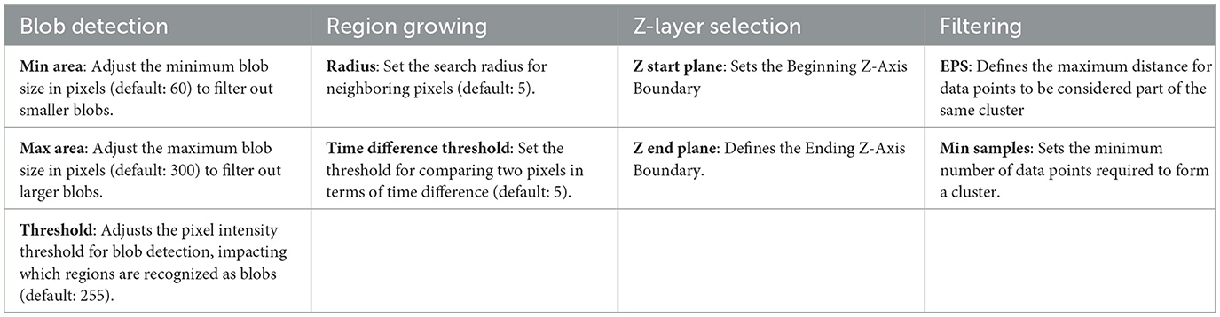
Table 1. Critical parameters configured by user.
The differences in MHIs generated from raw holograms vs. maximum-Z projections of the reconstructions are significant. Directly generated MHIs show fewer, thicker paths since only the organisms swimming close to the focal plane were detected (Figure 3A). MHIs from max-Z projections show many more paths, depending on the selected reconstruction depth. The paths are thinner because particles in focus appear smaller than their out-of-focus Airy spots and rings. The choice of projection depth is determined by cell density and noise, with projections of more focal planes leading to more noise (Figures 3B, C). Figures 3D–F shows DS3 where eleven microbes were hand-tracked, but only two of them showed active motility. The motile tracks were tracked accurately by the region-growing algorithm applied to the hologram MHI. The tracking of the non-motile microbes, which appear as blobs in the MHI, was not as accurate and required a strong adjustment of the threshold parameters.
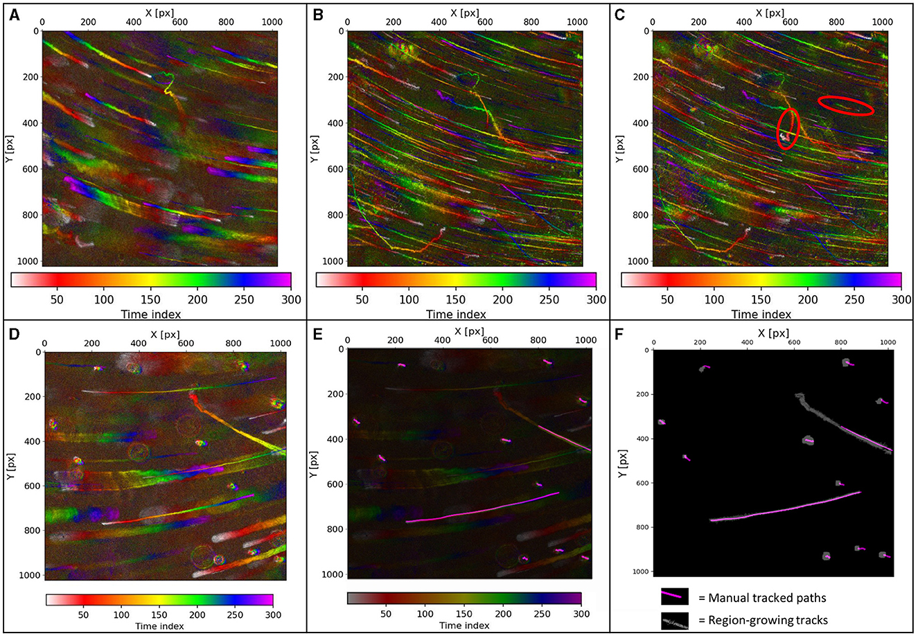
Figure 3. Holograms of DS2. (A) Hologram MHI. (B) Max-Z projection MHI of 49 Z-planes. (C) Max-Z projection MHI of 77 Z-planes. Tracks that are not visible in (B) are in (C) outlined in red. There is more noise in (C) than in (B). The paths in (A) are thicker but fewer paths are visible than in (B, C). (D) DS3 Hologram-MHI of DS3. (E) Hologram-MHI with an overlay of the hand-labeled tracks. (F) The tracks found by the region growing algorithm were applied to the hologram MHI (white) with an overlay of the hand-labeled tracks (purple). The two long motile tracks are tracked fully. The non-motile microbes have been partially tracked only.
Figure 4A shows the max-Z MHI of DS1, consisting of 851 timeframes and a depth of 404 μm. Figure 4B shows Track 9 from DS1. The wrong parameter selection (radius and threshold) of the region growing algorithm led to either incomplete tracking in a maximum-Z projection MHI or to spreading out and assigning too many pixels. The robustness of the parameter choice depended on many factors: the density of microbes, their speeds, the degree of noise, the reconstruction depth, and the length of the recording. In general, the larger the parameters were, the more is tracked, which can be helpful to skip gaps in the tracks in the MHI or to avoid large speed gaps. At the same time, larger parameters increase the probability of assigning unassociated regions to single tracks. These can be separated by later filters and clustering techniques. In summary, the region growing algorithm works particularly well when fast, uncrossed microbes are to be tracked. Here, a low radius and low threshold can be used. For non-motile, barely moving microbes, the threshold must be increased drastically.
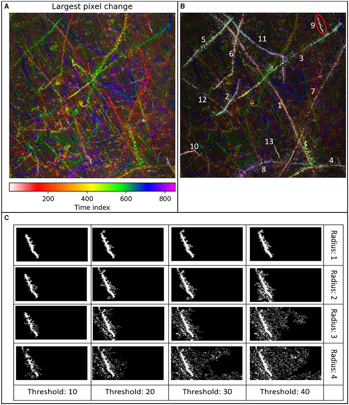
Figure 4. (A) Max-Z MHI of DS1, 851 timeframes, depth of 404 μm. The field of view is 365 μm × 365 μm. (B) Exemplary detection of 13 tracks with the region growing algorithm overlayed on the maximum Z-projection MHI of DS1. The maximum z-projection that was used for this MHI had plane distances of 4 μm, 851 time points, i.e., 56 seconds. (C) Track 9 found by region growing with different radii and thresholds, no overlay, no post-processing. Increasing the radius and threshold leads generally to a stronger spreading of the region. The combination of radius 4, with thresholds 30 and 40 leads to a spreading about the whole 365 μm × 365 μm FOW. Note that the increase in threshold is in 10-value steps, the increase of radius in single steps.
Filtering and clustering are crucial, especially in cases where the region-growing algorithm does not yield an unambiguous single microbial path. Figure 5 shows an example of a track from DS1 using the region growing parameters radius = 3 and threshold = 9. The resulting track segment consists of at least two different tracks identified as one region. Based on the color-coded temporal change, it can be seen that two other tracks also lay within the identified region (Figure 6D).
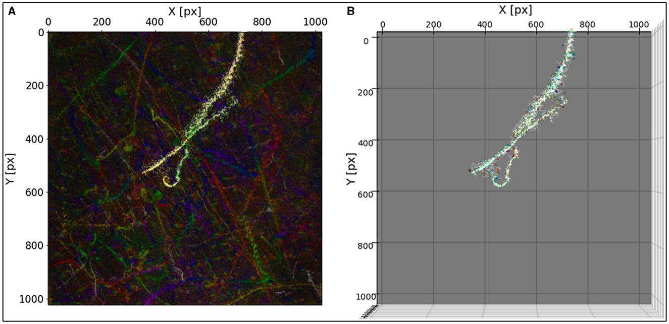
Figure 5. (A) A track found by the region-growing algorithm overlayed on MHI. (B) The same track in (A) overlayed on detected particles in 3D view parallel to the Z axis. The seed point was at X = 377 and Y = 188. The parameters of the region growing are radius = 3, and threshold = 9.
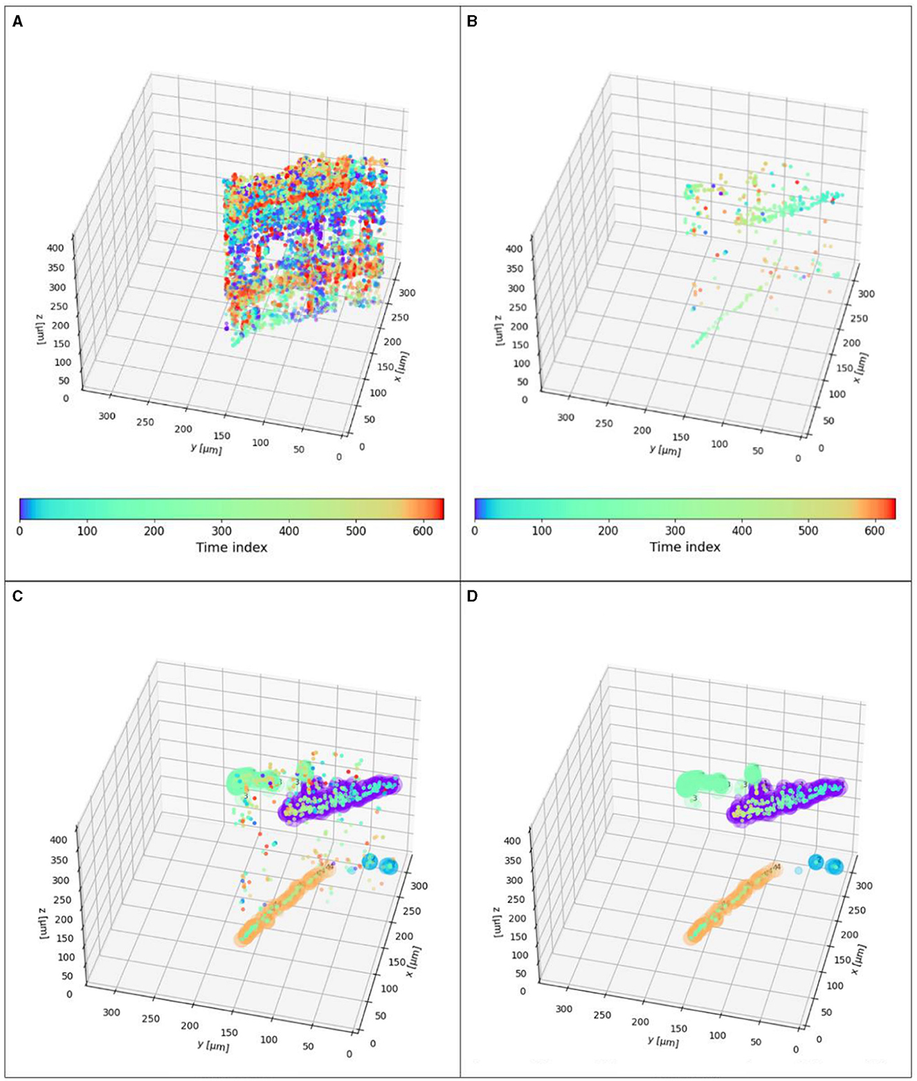
Figure 6. XYZt values of microbes (same as highlighted track in Figure 9): (A) Particles over all time points. (B) Particles with a maximum difference of 5 timeframes. They are compared to the corresponding MHI values. 365 μm in X and Y are the same as 1,024 px in the previous figures. Although DS1 contains 851 time values, the tracked particles here only comprise ~610 time values. (C) Results of DBSCAN (ε-value = 0.15, min_samples = 10) applied to the track shown in Figures 5A, B. Four tracks and 190 outliers (noise points). (D) Same results but without the outliers.
Figure 6 shows the results of the detected blobs in 3D. Figure 6A shows the 3D positions of all detected blobs over all time points that lay on the 2D track segment. Many of these blobs are not part of the track, and the results are expectedly very noisy. This is because at any given timeframe blobs are detected which are only noise. To eliminate unrelated particles, we take advantage of the time-coding of the MHI and take only candidates who are near the same position at nearly the same time. As with spatial segmentation, we can adjust the allowed time difference to accommodate both system noise and between-frame particle motion. For example, in Figure 6B, only particles within a maximum difference of 5 timeframes (=0.33 seconds) are considered. Figure 6C shows the results of DBSCAN, Figure 6D shows the same result, without the filtered outliers. While the region growing algorithm took the XYt dimensions into account, the DBSCAN clusters additionally in the Z axis. The results depend on the distance metric and the maximum distance allowed for a point to be considered a part of a cluster.
Clustering with DBSCAN is based on predefined distance and density metrics. The algorithm identifies points that lay in low-density regions which are—according to our metric—spatially and/or temporally far apart from any identified cluster and were too few to form their own cluster and hence these points are marked as noise. The points are treated as 4-dimensional vectors (X, Y, Z, and t) which are first normalized along all dimensions. Following normalization, we specifically adjust the scale of the Z-dimension, making it four times larger than the others. This gives the Z-position of each blob more importance while clustering. The rationale for scaling along the Z-dimension is based on the understanding that prior steps already utilize the other dimensions—X,Y, and t—to distinguish between tracks with overlapping projections. We use the l2-norm of the difference between any two scaled points as the distance metric. Any two points with a distance less than a predefined value (ε) are considered to be in the same cluster. Any group of points with less than a predefined value (min_samples) is considered noise.
We compare the tracking results of the final output with manual tracking of the max-Z projections. For the manual tracking, we used the commonly used software Fiji (Schindelin et al., 2012). Furthermore, we compare the tracking results of our software with the results of the Fiji plugin TrackMate (Tinevez et al., 2017; Ershov et al., 2022), which is often used for automated tracking.
The tracking accuracy on DS1 is shown in Figure 7A and of DS2 in Figure 7B. Here, the results of manual tracking served as the ground truth. The mean pixel differences of the X and Y coordinates are shown for all the tracks. For DS1, all the tracks exhibit a mean difference smaller than 48 pixels (track 7), which is similar to the length of the microbe of track 7 in the max-z projection (40 pixels), whereas most of the microbes have a mean difference of below 10 pixels compared to manual tracking. The tracking of DS2 exhibits for all tracks except for track 8 mean differences below 4 pixels. Track 8 has a slightly higher mean difference, due to its bigger blob size. The differences in track accuracies of DS1 and DS2 can be explained by different reconstruction depths. DS1 has a depth of 404 μm, and DS2 a depth of 308 μm, which leads to a better signal-to-noise ratio at DS2. For comparison with TrackMate, we tried numerous parameters of different preprocessing and tracking steps (see Supplementary material for details of input and tracking methods, parameters, and results). The input data for TrackMate was preprocessed including a combination of thresholding, gaussian filtering, and sharpening. Additionally, for a better comparison of the tracking methods, we also used the blobs found by our software as input. The tracking methods we applied here were Simple LAP tracker, LAP tracking, and Kalman tracking. DS1 is too noisy to get good tracks with TrackMate. On DS2 TrackMate performed better, but the best results with TrackMate were sparser than the tracks detected by our software (Figure 8). Track stitching had to be performed more often compared to the results of our software. TrackMate achieved its optimal performance at DS2 when it utilized a combination of our blob detection outputs as input along with Kalman tracking but were still inferior to our approach presented above. The advantage of our approach lies in the combination of Motion History Images with region growing and blob detection. Low SNR leads to pathways that are not trackable using traditional tracking approaches. The noise leads also to a large number of blobs in our blob detection, but in the spatiotemporal comparison with the MHIs, this leads to clear and distinguishable tracks. It is inherent to the MHIs that they are robust in terms of visualizing tracks, even when there is a low signal-to-noise ratio. A further advantage of our software lies in the compartmentalized work-through for the single tracks. The traditional methods use tracking parameters for all of the potential tracks. Through the region-growing step, our software is better for dealing with datasets with a higher variance of microbial swimming speeds and patterns. This may be valuable in tracking mixed populations of microbes in laboratory and field samples and reduces time for data analysis significantly.
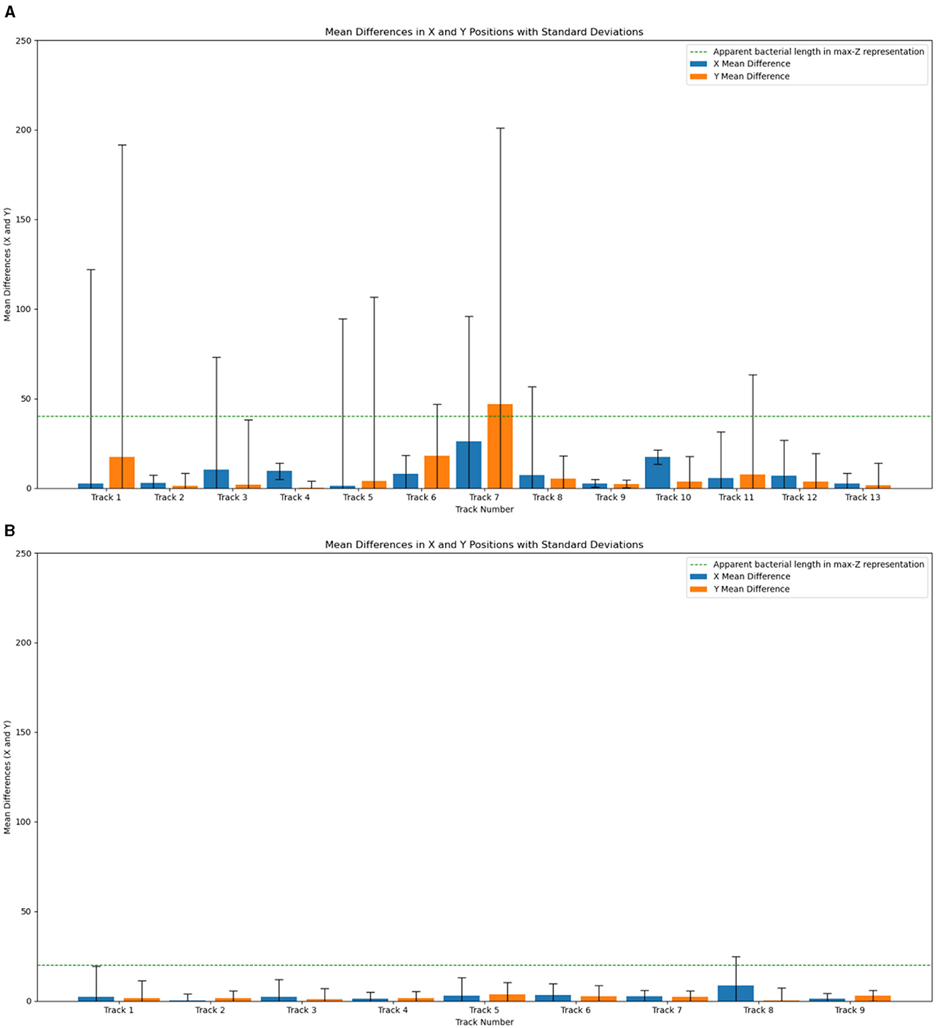
Figure 7. 2D tracking accuracy of our results compared with manual tracking for DS1 in (A) and for DS2 in (B). Stronger spreading of the region growing results at tracks 1, 3, 5, and 7 lead to a higher variance of the mean differences. The presence of noise in the maximum-Z projections may potentially lead to inaccuracies in manual tracking processes.
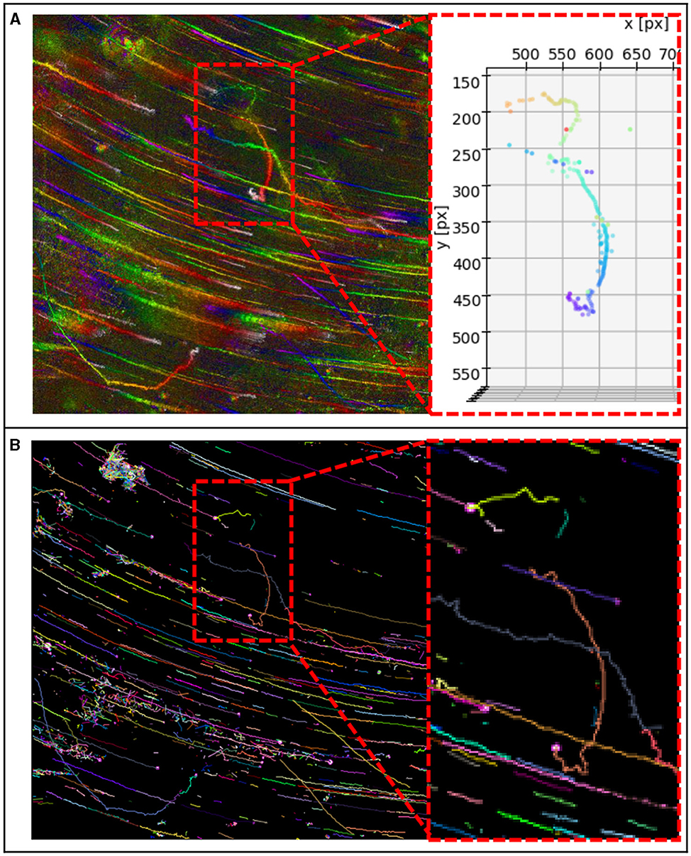
Figure 8. (A) MHI of DS 2 and details of track 7 found with our method. Consists of one track, without track stitching. (B) Tracks found with our blob detection as input and TrackMate's best result (Kalman Tracker, see Supplementary material for parameters). Here the same track consists of four single tracks, which must be stitched.
The accuracy of localization in depth is constrained by the system's depth of field (DOF), which in turn is determined by the wavelength (λ) used and the numerical aperture (NA) of the system:
With λ = 405 nm and NA = 0.31, this leads to a DOF of 4.2 μm. this leads to a DOF of 4.2 μm, Consequently, we utilized reconstruction layers spaced 4 μm apart from each other. Figure 9 shows Z-layer selection using the Tenengrad metric applied to the crops shown in gray (DS2). Additionally, we show the average brightness of crops that have at least one pixel with a minimum brightness of 80. The minimum brightness is required because very blurry images that do not represent particles often have a high average brightness. The Tenengrad metric gives overall the best results for all datasets presented here.
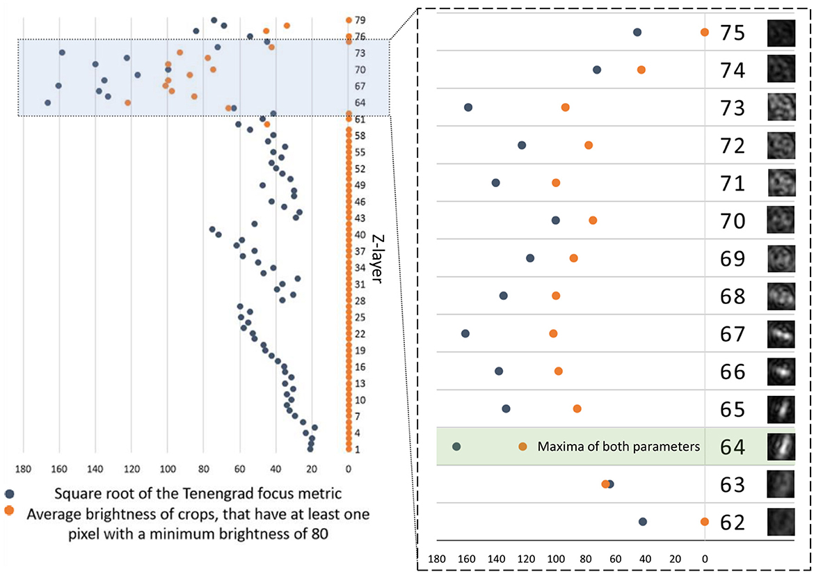
Figure 9. Square root of the Tenengrad and focus metric (gray). Average brightness of Z-layer crops, that have at least one pixel with a brightness of 80 (orange) depending on the Z-layer. Shown is time point 40 from DS2 with X = 328 and Y = 276 (for a dimension of 2,048 px × 2,048 px of the reconstructions). Left side: Each Z-layer has a distance of 4 μm to the next. Z-layers 1–79 comprise a depth of 316 μm. Right side: A section of the graph with the Z-layers 61–74 (depth of 52 μm) with the corresponding crops (28 × 28 px). Both parameters have their maxima at Z-layer 64, indicating the best focus and thus depth for that object. For the square root of the Tenengrad focus metric an area of 28 × 28 px was used (same as shown crops). For the average brightness of crops, that have at least one pixel with a brightness of 80 an area of 14 × 14 px was used. If the parameters use the respective other area sizes, both have their maximum in Z-layer 66 in this example. Z-layer 71 also has a relatively high brightness value, although it is visibly nowhere near a microbe.
In order to fully investigate Z-plane selection, we compare results from rod-shaped B. subtilis (2–6 μm long and < 1 μm in diameter) with those using Chlamydomonas, a larger (3–10 μm) photosynthetic microalga (DS4). The chlorophyll in this organism causes it to absorb strongly at our 405 nm illumination wavelength (Nadeau et al., 2016; Cohoe et al., 2019). Figures 10A–C show Z-layer selection for three different Chlamydomonas algae at an exemplary time point. The images show the results of the Z-layer selection of the two metrics using the large and small cut, respectively. The small cut has the same edge length as the diameter of the blob of the corresponding maximum-Z projection. The large crop has twice the edge length. The correctly selected Z-layers are outlined in green. They were selected from 79 Z-Layers. The particle in Figure 10D is a bacterium found in the Chlamydomonas culture. For the algae, the Tenengrad metric worked best due to the highly absorptive chloroplast. The small Tenengrad metric provided reliable results and was largely agnostic as to the type of particle to be found. For the bacterium in the same culture, the Tenengrad and brightness metrics are comparable. The small Tennengrad metric Z-layer selection for a microbe moving over 120 μm is shown in Figure 11 (DS1, track 2).
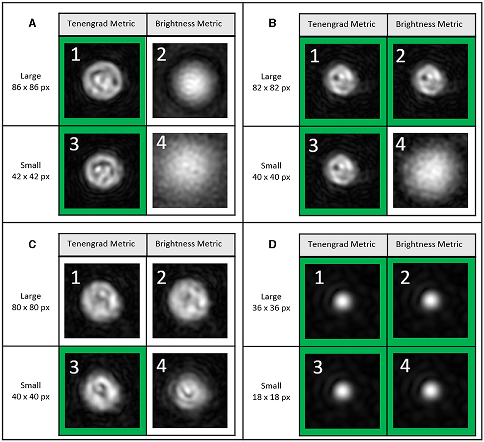
Figure 10. DS4, timepoint 29, Z-layer selection of three different Chlamydomonas algae (A–C) and one bacterium (D) from 101 Z-layers (=400 μm). The green square indicates the best selection out of the 101 Z-layers. (A) (1) Tenengrad metric, large, i.e., in this case 86 × 86 px, selected Z-layer: 45. (2) Brightness metric, large, i.e., 86 × 86 px, selected Z-layer: 69. (3) Tenengrad metric, small, i.e., in this case 42 × 42 px., selected Z-layer layer: 46. (4) Brightness metric, small, i.e., in this case 42 × 42 px., selected Z-layer: 12. It is not clear whether layer 45 or 46 is more accurate. (B) (1) Selected Z-layer: 76. (2) Selected Z-layer: 76. (3) Selected Z-layer layer: 76. (4) Selected Z-layer: 101. (C) (1) Selected Z-layer: 16. (2) Selected Z-layer: 15. (3) Selected Z-layer layer: 18. (4) Selected Z-layer: 13. (D) (1) Selected Z-layer: 39. (2) Selected Z-layer: 39. (3) Selected Z-layer layer: 39. (4) Selected Z-layer: 39. For the sake of clarity, the same size for the field of view is shown in (A): 86 × 86 px, i.e., 15 × 15 μm. (B) 82 × 82 px, i.e., 14.6 × 14.6 μm, (C) 80 × 80 px, i.e., 14.3 × 14.3 μm, (D): 36 × 36 px, i.e., 6.4 × 6.4 μm. Further information in Supplementary material.
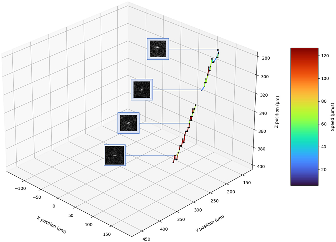
Figure 11. Track 2 of DS1 in 3D. The crops show the microbe at the selected Z-layer. Three wrongly detected blobs were manually removed (see Supplementary material).
Detection time was evaluated using an artificially generated 1024 px × 1024 px image containing only a white square of 100 px × 100 px. The seed point was set in the center. Doubling the radius resulted in a 4-fold increase of the detection time, indicating an quadratic relationship between the number of pixel neighbors to be checked (r∧2-1) and the detection time. Table 2 shows the detection times for the track regions of DS1. The detection values of a track depend on the radius and the track length. Table 3 gives an overview of user work time and computational requirements to process datasets.
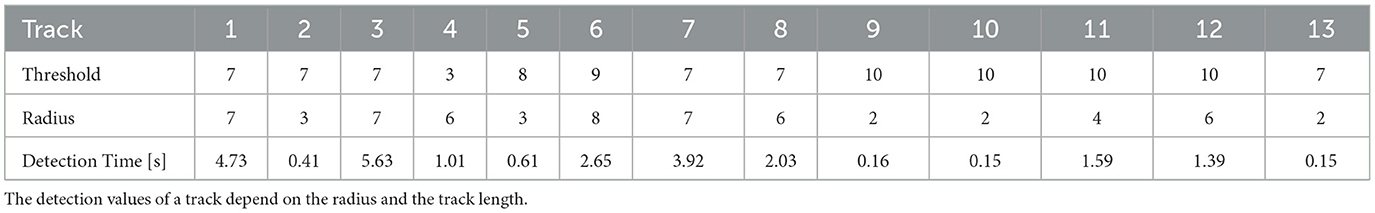
Table 2. Segmentation times for the tracks shown in Figure 4A performed on a notebook with Intel(R) Core (TM) i7-10510U CPU @ 1.80GHz 2.30 GHz and 32.0 GB RAM.
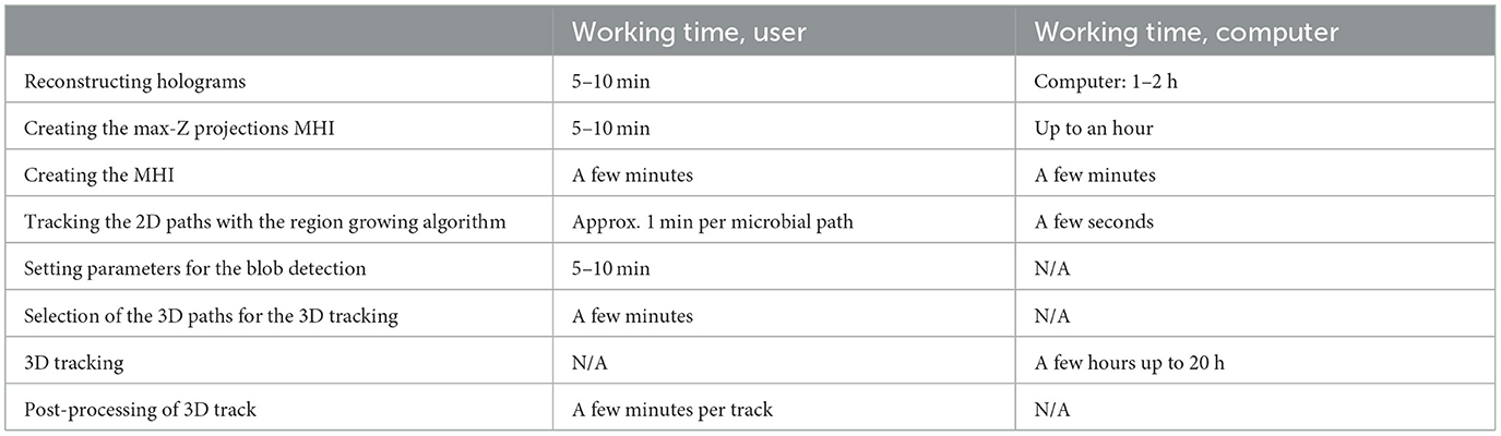
Table 3. Processing time required by both the user and the computer to analyze a dataset using our tracking approach, spanning approximately 900 frames performed on a notebook with Intel(R) Core (TM) i7-10510U CPU @ 1.80GHz 2.30 GHz and 32.0 GB RAM.
This software can create accurate and clear prokaryotic pathways in 3D, even if the holograms and reconstructions have a low signal-to-noise ratio (Figure 12). Furthermore, it can handle datasets containing microbes of different body sizes (DS4). Region growing is suitable for detecting two-dimensional microbial pathways in MHIs generated from DHM recordings, either raw holograms or Z-projected reconstructions. It is a useful tool for automated tracking and analysis of microbial motility and is capable of tracking individual microbes that exhibit high variations in their swimming speed and direction. In our comparison to traditional automated tracking methods, it was more accurate and faster. Our software greatly speeds up the work process compared to manual tracking and its advantage is even greater when the third spatial dimension is considered. In combination with the reconstructed images, it proved to be very useful for tracking microbes in 3D. Especially for tracking highly noisy data sets it seems to be more suitable for tracking compared to traditional methods.
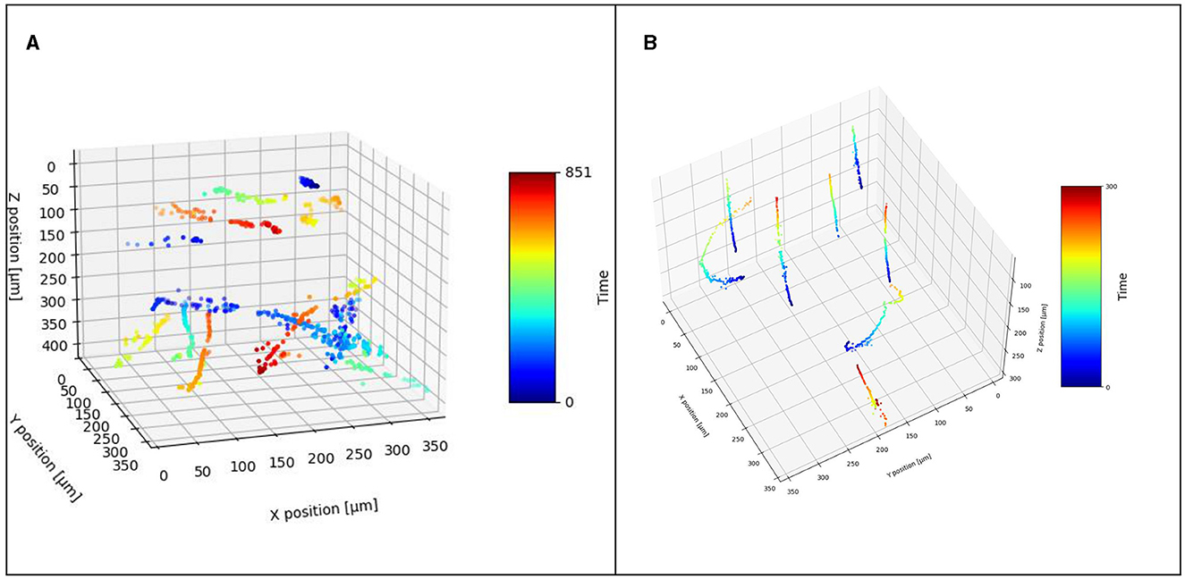
Figure 12. Detected 3D track from (A) DS1 and (B) DS2.
The next steps for improvement are to fully automate the work steps in which the human user interacts. This involves finding easy-to-implement heuristics for automating the selection of the reconstruction area, and the parameters of the region growing algorithm. Full automation can most likely be realized using traditional image analysis processes at low computational cost.
Further steps for the improvement of the software comprise refined Z-layer selection. We showed that we are capable of tracking 15–25 μm/s fast swimming 2–6 μm long, rod-shaped prokaryotes with our optical setup with a camera with 15 frames per second. Twenty five μm/s corresponds to tracking objects at speeds of 9 px/frame. However, future work has to test the limits of cell size, speed, and density, which have not yet been fully determined yet, and further research is required to establish these parameters. Finding optimal parameters for specific optics, hardware, and microbes is crucial to ensure accurate and reliable analysis. In future work, we will implement an automated extraction of motility features in 3D and allow for setting optimal parameters such as threshold and radius depending on the specifics of the optical setup (e.g., camera frame rate, magnification), and microbial species. Automated motility analysis will include the identification of the type of swimming and the number of runs, tumbles, and reversals. Currently, the software also lacks an easy-to-use GUI which is important so that it can be used by a larger group of scientists and other end users.
Despite these limitations, the software provides a foundation for low-cost motility analysis and research with big data, as it can process and analyze large amounts of data quickly. It might enable researchers to identify subtle changes in motility patterns and provide insights into the underlying biology.
The software is available online at: https://github.com/maxriek/3D-Microbe-Tracking Project name: 3D-Microbe-Tracking.
MR: Conceptualization, Funding acquisition, Investigation, Methodology, Software, Validation, Visualization, Writing—original draft, Writing—review & editing. HA: Software, Validation, Writing—original draft, Writing—review & editing. MD: Data curation, Writing—original draft, Writing—review & editing. JN: Conceptualization, Resources, Supervision, Validation, Writing—original draft, Writing—review & editing, Methodology. CL: Conceptualization, Funding acquisition, Methodology, Resources, Supervision, Validation, Writing—original draft, Writing—review & editing.
The author(s) declare that financial support was received for the research, authorship, and/or publication of this article. This work was financially supported in part by the Friedrich Ebert Foundation. Portions of this work were performed at, or funded by, the Jet Propulsion Laboratory, California Institute of Technology, under contract with the National Aeronautics and Space Administration.
We wish to thank Mark Wronkiewicz, Jake Lee, and Nikki Johnston for helpful discussions regarding the HELM software.
The authors declare that the research was conducted in the absence of any commercial or financial relationships that could be construed as a potential conflict of interest.
The author(s) declared that they were an editorial board member of Frontiers, at the time of submission. This had no impact on the peer review process and the final decision.
All claims expressed in this article are solely those of the authors and do not necessarily represent those of their affiliated organizations, or those of the publisher, the editors and the reviewers. Any product that may be evaluated in this article, or claim that may be made by its manufacturer, is not guaranteed or endorsed by the publisher.
The Supplementary Material for this article can be found online at: https://www.frontiersin.org/articles/10.3389/fimag.2024.1393314/full#supplementary-material
Berg, H. C., and Anderson, R. A. (1973). Bacteria swim by rotating their flagellar filaments. Nature 245, 380–382. doi: 10.1038/245380a0
Berg, H. C., and Brown, D. A. (1972). Chemotaxis in Escherichia coli analysed by three-dimensional tracking. Nature 239, 500–504. doi: 10.1038/239500a0
Berg, H. C., and Brown, D. A. (1974). Chemotaxis in Escherichia coli analyzed by three-dimensional tracking. Antibiot Chemother. 19, 55–78. doi: 10.1159/000395424
Burri, O. (2018). Image Stack Equalizer for Image Folder. Available online at: https://gist.github.com/lacan/3de16eb24f954399b763445070fe4bfc (accessed March 1, 2023).
Cheong, F. C., Wong, C. C., Gao, Y., Nai, M. H., Cui, Y., Park, S., et al. (2015). Rapid, high-throughput tracking of bacterial motility in 3D via phase-contrast holographic video microscopy. Biophys. J. 108, 1248–1256. doi: 10.1016/j.bpj.2015.01.018
Cohoe, D., Hanczarek, I., Wallace, J. K., and Nadeau, J. (2019). Multiwavelength digital holographic imaging and phase unwrapping of protozoa using custom fiji plug-ins. Front. Phys. 7:94. doi: 10.3389/fphy.2019.00094
Dubay, M. M., Acres, J., Riekeles, M., and Nadeau, J. L. (2022a). Recent advances in experimental design and data analysis to characterize prokaryotic motility. J. Microbiol. Methods 204:106658. doi: 10.1016/j.mimet.2022.106658
Dubay, M. M., Johnston, N., Wronkiewicz, M., Lee, J., Lindensmith, C. A., and Nadeau, J. L. (2022b). Quantification of motility in Bacillus subtilis at temperatures Up to 84°C using a submersible volumetric microscope and automated tracking. Front. Microbiol. 13:836808. doi: 10.3389/fmicb.2022.836808
Ershov, D., Phan, M.-S., Pylvänäinen, J. W., Rigaud, S. U., Le Blanc, L., Charles-Orszag, A., et al. (2022). TrackMate 7: integrating state-of-the-art segmentation algorithms into tracking pipelines. Nat. Methods 19, 829–832. doi: 10.1038/s41592-022-01507-1
Farthing, N. E., Findlay, R. C., Jikeli, J. F., Walrad, P. B., Bees, M. A., and Wilson, L. G. (2017). Simultaneous two-color imaging in digital holographic microscopy. Opt. Expr. 25, 28489–28500. doi: 10.1364/OE.25.028489
Helmli, F. S., and Scherer, S. (2001). “Adaptive shape from focus with an error estimation in light microscopy,” in ISPA 2001. Proceedings of the 2nd International Symposium on Image and Signal Processing and Analysis. In conjunction with 23rd International Conference on Information Technology Interfaces (IEEE), 188–193.
Jaqaman, K., Loerke, D., Mettlen, M., Kuwata, H., Grinstein, S., Schmid, S. L., et al. (2008). Robust single-particle tracking in live-cell time-lapse sequences. Nat. Methods 5, 695–702. doi: 10.1038/nmeth.1237
Johnston, N., Dubay, M., Wronkiewicz, M., Lee, J., Lindensmith, C., and Nadeau, J. (2022). Raw holograms frames of Bacillus Subtilis at different temperatures. Available online at: https://datadryad.org/stash/dataset/ (accessed March 1, 2023).
Kim, M. K. (2010). Principles and techniques of digital holographic microscopy. J. Photon. Energy 1:18005. doi: 10.1117/6.0000006
Kühn, M. J., Schmidt, F. K., Farthing, N. E., Rossmann, F. M., Helm, B., Wilson, L. G., et al. (2018). Spatial arrangement of several flagellins within bacterial flagella improves motility in different environments. Nat. Commun. 9:5369. doi: 10.1038/s41467-018-07802-w
Li, X., Wang, K., Wang, W., and Li, Y. (2010). “A multiple object tracking method using Kalman filter,” in The 2010 IEEE International Conference on Information and Automation (IEEE), 1862–1866. doi: 10.1109/ICINFA.2010.5512258
Liu, B., Gulino, M., Morse, M., Tang, J. X., Powers, T. R., and Breuer, K. S. (2014). Helical motion of the cell body enhances Caulobacter crescentus motility. Proc. Natl. Acad. Sci. U S A 111, 11252–11256. doi: 10.1073/pnas.1407636111
Martinez-Baena, J., Fdez-Valdivia, J., and García, J. A. (1997). A multi-channel autofocusing scheme for gray-level shape scale detection. Patt. Recogn. 30, 1769–1786. doi: 10.1016/S0031-3203(96)00194-X
Molaei, M., Barry, M., Stocker, R., and Sheng, J. (2014). Failed escape: solid surfaces prevent tumbling of Escherichia coli. Phys. Rev. Lett. 113:68103. doi: 10.1103/PhysRevLett.113.068103
Nadeau, J. L., Cho, Y. B., Kühn, J., and Liewer, K. (2016). Improved tracking and resolution of bacteria in holographic microscopy using dye and fluorescent protein labeling. Front. Chem. 4:17. doi: 10.3389/fchem.2016.00017
Schindelin, J., Arganda-Carreras, I., Frise, E., Kaynig, V., Longair, M., Pietzsch, T., et al. (2012). Fiji: an open-source platform for biological-image analysis. Nat. Methods 9, 676–682. doi: 10.1038/nmeth.2019
Schubert, E., Sander, J., Ester, M., Kriegel, H. P., and Xu, X. (2017). DBSCAN revisited, revisited. ACM Trans. Datab. Syst. 42, 1–21. doi: 10.1145/3068335
Schuech, R., Hoehfurtner, T., Smith, D. J., and Humphries, S. (2019). Motile curved bacteria are Pareto-optimal. Proc. Natl. Acad. Sci. U S A 116, 14440–14447. doi: 10.1073/pnas.1818997116
Sheng, J., Malkiel, E., Katz, J., Adolf, J., Belas, R., and Place, A. R. (2007). Digital holographic microscopy reveals prey-induced changes in swimming behavior of predatory dinoflagellates. Proc. Natl. Acad. Sci. U S A 104, 17512–17517. doi: 10.1073/pnas.0704658104
Tang, M., He, H., and Yu, L. (2022). Real-time 3D imaging of ocean algae with crosstalk suppressed single-shot digital holographic microscopy. Biomed. Opt. Expr. 13, 4455–4467. doi: 10.1364/BOE.463678
Thornton, K. L., Butler, J. K., Davis, S. J., Baxter, B. K., and Wilson, L. G. (2020). Haloarchaea swim slowly for optimal chemotactic efficiency in low nutrient environments. Nat. Commun. 11:4453. doi: 10.1038/s41467-020-18253-7
Tinevez, J.-Y., Perry, N., Schindelin, J., Hoopes, G. M., Reynolds, G. D., Laplantine, E., et al. (2017). TrackMate: an open and extensible platform for single-particle tracking. Methods 115, 80–90. doi: 10.1016/j.ymeth.2016.09.016
Turner, L., Ping, L., Neubauer, M., and Berg, H. C. (2016). Visualizing flagella while tracking bacteria. Biophys. J. 111, 630–639. doi: 10.1016/j.bpj.2016.05.053
Wallace, J. K., Rider, S., Serabyn, E., Kühn, J., Liewer, K., Deming, J., et al. (2015). Robust, compact implementation of an off-axis digital holographic microscope. Opt. Expr. 23, 17367–17378. doi: 10.1364/OE.23.017367
Wang, A., Garmann, R. F., and Manoharan, V. N. (2016). Tracking E. coli runs and tumbles with scattering solutions and digital holographic microscopy. Opt. Expr. 24, 23719–23725. doi: 10.1364/OE.24.023719
Wilson, L., and Zhang, R. (2012). 3D Localization of weak scatterers in digital holographic microscopy using Rayleigh-Sommerfeld back-propagation. Opt. Expr. 20:16735. doi: 10.1364/OE.20.016735
Wronkiewicz, M., and Lee, J. (2021). Holographic Examination for Life-like Motility (HELM): MHI generator. Available online at: https://github.com/JPLMLIA/OWLS-Autonomy (accessed September 21, 2022).
Wronkiewicz, M., Lee, J., Lightholder, J., Mauceri, S., Kim, T., McKinney, S., et al. (2022). Dataset for “Identifying and Characterizing Motile and Fluorescent Microorganisms in Microscopy Data Using Onboard Science Autonomy”. doi: 10.48577/jpl.2KTVW5
Wronkiewicz, M., Lee, J., Mandrake, L., Lightholder, J., Doran, G., Mauceri, S., et al. (2024). Onboard science instrument autonomy for the detection of microscopy biosignatures on the ocean worlds life surveyor. Planet. Sci. J. 5:19. doi: 10.3847/PSJ/ad0227
Xiong, Y., and Shafer, S. A. (1993). “Depth from focusing and defocusing,” in Proceedings of IEEE Conference on Computer Vision and Pattern Recognition, 68–73. doi: 10.1109/CVPR.1993.340977
Keywords: 3D tracking, quantitative tracking, digital holographic microscopy, microbial motility, microscopy, region growing, microswimmers
Citation: Riekeles M, Albalkhi H, Dubay MM, Nadeau J and Lindensmith CA (2024) Motion history images: a new method for tracking microswimmers in 3D. Front. Imaging. 3:1393314. doi: 10.3389/fimag.2024.1393314
Received: 28 February 2024; Accepted: 24 April 2024;
Published: 10 May 2024.
Edited by:
Byung-Gyu Kim, Sookmyung Women's University, Republic of KoreaReviewed by:
Laurence Wilson, University of York, United KingdomCopyright © 2024 Riekeles, Albalkhi, Dubay, Nadeau and Lindensmith. This is an open-access article distributed under the terms of the Creative Commons Attribution License (CC BY). The use, distribution or reproduction in other forums is permitted, provided the original author(s) and the copyright owner(s) are credited and that the original publication in this journal is cited, in accordance with accepted academic practice. No use, distribution or reproduction is permitted which does not comply with these terms.
*Correspondence: Max Riekeles, cmlla2VsZXNAdHUtYmVybGluLmRl
†Present address: Megan Marie Dubay, Department of Physics and Astronomy, University of North Carolina at Chapel Hill, Chapel Hill, NC, United States
Disclaimer: All claims expressed in this article are solely those of the authors and do not necessarily represent those of their affiliated organizations, or those of the publisher, the editors and the reviewers. Any product that may be evaluated in this article or claim that may be made by its manufacturer is not guaranteed or endorsed by the publisher.
Research integrity at Frontiers
Learn more about the work of our research integrity team to safeguard the quality of each article we publish.