 Fernando Galaz Prieto
 Maryam Samavaki
 Sampsa Pursiainen
- Computing Sciences, Faculty of Information Technology, Tampere University, Tampere, Finland
Introduction: This study focuses on broadening the applicability of the metaheuristic L1-norm fitted and penalized (L1L1) optimization method in finding a current pattern for multichannel transcranial electrical stimulation (tES). The metaheuristic L1L1 optimization framework defines the tES montage via linear programming by maximizing or minimizing an objective function with respect to a pair of hyperparameters.
Methods: In this study, we explore the computational performance and reliability of different optimization packages, algorithms, and search methods in combination with the L1L1 method. The solvers from Matlab R2020b, MOSEK 9.0, Gurobi Optimizer, CVX's SeDuMi 1.3.5, and SDPT3 4.0 were employed to produce feasible results through different linear programming techniques, including Interior-Point (IP), Primal-Simplex (PS), and Dual-Simplex (DS) methods. To solve the metaheuristic optimization task of L1L1, we implement an exhaustive and recursive search along with a well-known heuristic direct search as a reference algorithm.
Results: Based on our results, and the given optimization task, Gurobi's IP was, overall, the preferable choice among Interior-Point while MOSEK's PS and DS packages were in the case of Simplex methods. These methods provided substantial computational time efficiency for solving the L1L1 method regardless of the applied search method.
Discussion: While the best-performing solvers show that the L1L1 method is suitable for maximizing either focality and intensity, a few of these solvers could not find a bipolar configuration. Part of the discrepancies between these methods can be explained by a different sensitivity with respect to parameter variation or the resolution of the lattice provided.
1 Introduction
Transcranial Electrical Stimulation (tES) is a non-invasive brain stimulation method used for stimulating neuronal activity, treating psychiatric disorders, and studying neuronal behavior by transmitting a constant low-intensity current pattern through a set of electrode patches attached to the scalp of the subject to modulate cortical excitability (Nitsche and Paulus, 2000). In tES, a volumetric current density in the brain is generated by injecting through the scalp a current pattern that can be described via different properties, including the number of active electrodes, their physical description (e.g., positioning, shape, permittivity, and impedance values), the applied stimulus waveform (e.g., amplitude, pulse shape, pulse width, and polarity), the number of stimulation sessions, and the time interval (Peterchev et al., 2012). Since different electrode montages result in distinct brain current flow, clinicians and researchers can adjust the montage to target or avoid specific brain regions in an application-specific manner.
An increasingly popular form of tES is the Transcranial Direct Current Stimulation (tDCS) method (Paulus, 2011; Moreno-Duarte et al., 2014; Thair et al., 2017; Reed and Cohen Kadosh, 2018). Compared to other non-invasive stimulation methods, the advantages of tDCS can be attributed to its inexpensive and approachable characteristics. Unlike the intricate machinery required for Transcranial Magnetic Stimulation (TMS) or the specialized frequency considerations in Transcranial Alternating Current Stimulation (tACS), tDCS involves a simpler setup—a direct current passed through scalp electrodes. This simplicity not only reduces the cost of equipment but also enhances portability, making tDCS more accessible for various settings, including home use. The simplicity and minimal training required contribute to its user-friendly nature enabling a broader range of individuals to utilize or participate in studies involving this method. Whereas tDCS is classically applied in a two-channel configuration (Kaufmann et al., 2021), its focality can be enhanced via multiple channels, which has motivated the introduction of advanced optimization methods for finding an optimal multi-channel montage (Fernandez-Corazza et al., 2020).
tES modeling involves constructing computational representations of the head and brain anatomy, simulating the distribution of electric fields. This process integrates factors such as electrode placement, tissue conductivity, and finite element method simulations to visualize and analyze the spatial distribution of the electric field within the brain. Generating a high-resolution forward model is critical for building an explicit patient-specific head model, determining optimal positioning of electrodes, and predicting electric field generation across the brain for specific stimulation configurations (Faria et al., 2011; Rampersad et al., 2013; Wagner et al., 2013). Using such a forward model, multi-electrode stimulation can be optimized via specifically designed mathematical methodology (Dmochowski et al., 2011; Ruffini et al., 2014; Guler et al., 2016; Wagner et al., 2016; Fernandez-Corazza et al., 2020), such as the recently developed convex optimization schemes including the Distributed Constrained Maximum Intensity (D-CMI) (Khan et al., 2022), and the metaheuristic L1-norm regularized L1-norm fitting (L1L1) (Galaz Prieto et al., 2022) which aim at an individualized distributional fit for a given target activity.
In this study, we aim to broaden the applicability of the linear programming (LP)-based L1L1 method for finding tES electrode montages computationally in a comprehensive manner, i.e., by evaluating the metaheuristic results and total computing time through different mathematical optimization algorithms and packages; this includes Interior-Point (IP) (Mehrotra, 1992), Primal-Simplex (PS), and Dual-Simplex (DS) (Boyd and Vandenberghe, 2004) as alternative LP algorithms, and Matlab (R2020b) from MathWorks (Zhang, 1999), MOSEK Optimization Suite (Release 9.0) (Mosek, 2019), Gurobi Optimization (9.5.1) (Gurobi Optimization LLC, 2022), SDPT3 (4.0) (Tütüncü et al., 2003), and SeDuMi (1.3.5) (Sturm, 1999; Frenk et al., 2000; Polik et al., 2007) as alternative packages. The latter two open-source alternatives are available in the CVX optimization toolbox (Grant and Boyd, 2014). We also investigate the metaheuristic hyperparameter optimization (HPO) task of L1L1 via exhaustive search (Bianchi et al., 2009) and recursive search (Je and Park, 2013) with heuristic direct search as a reference algorithm (Bogani et al., 2009).
Our results suggest that the performance differences between the above-mentioned optimization packages, algorithms, and search methodology can be crucial regarding the optimization results, focality stimulation current, and the availability of active channels in the montage. Moreover, exhaustive and recursive search methods can also be considered preferable to heuristic direct search in terms of their overall reliability and predictability.
2 Materials and methods
In tES, a real L × 1 current pattern y is injected into the subject's head through a set of contact electrodes attached to the scalp. These electrodes, ranging from 0.5 to 4.0 milliamperes (mA) (Zaghi et al., 2010; Khadka et al., 2020; Workman et al., 2020), form what is known as an electrode montage and are responsible for distributing the injected volumetric current density–measured in ampere per square meter (A/m2)–throughout the scalp, skull, cerebrospinal fluid (CSF), and brain components, including cortical and subcortical brain structures. The governing linear system is of the form
where is a real N × L lead field matrix (forward mapping) that describes the relationship between the y, and is a real N × 1 discretized volume current density vector. The linear system (Equation 1) is re-interpreted component-wise as the focused field , where the target field has non-zero values, and the nuisance field , where it vanishes. Detailed mathematical definition of the lead field matrix refer to Appendix A. Forward model in Galaz Prieto et al. (2022).
The optimization problem needs to find the best matching between y, and the focused field via Ly = x, where the projection of the focused field into the direction of the target constitutes the first component as
with P denoting a matrix that projects a vector into the direction of . The target amplitude ||x1||2 is set as 3.85 A/m2 which is an approximation of the excitation current threshold for nerve fibers of the upper limb area of the motor cortex (Kowalski et al., 2002).
2.1 L1-norm fitted and regularized optimization
The goal in L1-norm Fitted and Regularized (L1L1) optimization method (Galaz Prieto et al., 2022) is to minimize
The injection on every active ℓ-th electrode channel is limited to γ ≤ 2.0 mA, the total injection current dose flowing through the tES head cap is within the safety limit μ ≤ 4.0 mA, and the total sum of electric current from every active electrode channel in yℓ, where ℓ ∈ {1, ⋯ , L}, must be equal to zero. The regularization parameter α sets the level of L1-regularization with respect to the scaling value ζ = ||L||1. The function
where w = (w1, w2, ⋯ , wM), sets the nuisance field threshold 0 ≤ ε ≤ 1 with respect to the scaling value ν = ||x||∞, meaning that entries (L2y)m with an absolute value below εν do not actively contribute to the minimization process due to the threshold. We refer to the set {m:|(L2y)m| ≥ εν} as the constraint support, i.e., the index set contributing to the value of the objective function. Detailed formulation of the linear programming system (Equation 2) can be found in Galaz Prieto et al. (2022).
The current density Γ of the focused field is defined as
and the focality of the stimulus Θ is defined as the following current ratio
The metacriterion Γ ≥ Γ0 is applied to maintain appropriate intensity at the target location. Namely, without a lower bound for the intensity, the intensity of the maximizer is likely to vanish.
2.2 Two-stage metaheuristic lattice search
To derive a multi-channel tES montage following the aforementioned equations, the optimization framework takes into account the following indications: (A) a procedure for selecting the most relevant electrodes in the montage for a given region of interest; (B) a definition of the tuning parameters which will maximize or minimize the objective function; and (C) a method to evaluate said parameters and retrieve data (search method). In this study, 128 electrodes were attached to the scalp following the international 10-10 EEG hardware system with an impedance of 2.0 kOhm (kiloohms). Physiological impediments in the head model, fluctuation in conductivity tissue, and behavior of the injected current aspects are excluded. The framework of this search is as follows:
(A) The two-stage determines which of the tES channels in the neurostimulator headgear should be set as active or inactive based on the field distribution on the head surface for a given current source in the brain. After calculating the lead field matrix, the user specifies an approximate region of interest through forward dipole modeling (Bauer et al., 2015; Medani et al., 2015; Pursiainen et al., 2016). This is the highlighted region from which the two-stage procedure shall prioritize the electrode selection as follows:
(A.1). During the first stage, the optimization model sets all channels with an initial current of zero value and determines a volumetric current density influenced by the electric properties, direction, and positioning of the dipole modeling. Then, the optimization model filters the montage down to a (user-defined) number of electrodes that contribute the most to the maximal safety tES current injection based on the initial range of α and ε values provided. The corresponding electric potential from the now-limited montage with channels yℓ is normalized to meet the intended maximum current injection μ value while the remaining electrodes are opted out of further calculations. We constraint the total number of active electrodes available to ℓ = 20 inspired by commercial tES systems (Roy et al., 2019; Tost et al., 2021).
(A.2). In the second stage, the optimization re-runs using only the active electrodes obtained previously. In this stage, the objective function can be retroactively modified to retrieve a customized montage that favors an intense volumetric current density Γ or a maximal stimulation focality given a target current Θ. The final result is then thresholded to a non-zero number of currents in the pattern.
(B) Using metaheuristic methodology means developing an algorithm that can produce near-optimal results in a computationally feasible time (Bianchi et al., 2009). In the present context, the objective is to iteratively adjust the parameters α and ε to ascertain a solution that minimally impairs the objective function. The aim is to secure a heightened amplitude within the targeted focus field while concurrently mitigating undesirable signals (the nuisance field). We define a parameter space by specifying ranges for αm from -100 to -20 dB and εn from -160 to 0 dB, employing logarithmic increments. Plotting these parameter values on a Cartesian plane elucidates the search space κ, subject to a set of constraints delineated by the linear programming paradigm at hand.
(C) The lattice search aspect defines the instructions on how to retrieve information from the search space κ for solving (Equation 2). This task can be considered as a hyperparameter optimization (HPO) exercise (Feurer and Hutter, 2019; Yang and Shami, 2020) for building a predictive model that performs best when using the most fitting αm and εn parameters. The following exploration techniques are evaluated for finding these parameters: exhaustive search, direct search, and recursive search.
(C.1) The exhaustive search, or grid search, systematically evaluates every possible candidate solution within the search space κ, i.e., the Cartesian product of each αm and εn value in existence (Figure 1A). The final candidate solution is the combination that best minimizes the objective function. We applied a coarse grid of size κ = 15 and compared it against a finer grid of size κ = 40.
(C.2) By direct search, we refer to the Generalized direct search (GPS) (Bogani et al., 2009) available in the Matlab's optimization toolbox. It aims at finding a point in the hyperparameter space without knowledge of any gradient. The method begins with a given search window D(i) and an initial estimate acting as a pivot. The location of this window is centralized over the pivot along with its four orthogonal neighbor points in the Euclidian distance w(i), i.e.,
Figure 1B depicts the mesh and its behavior. At each i-th iteration within the mesh, if a neighboring point performs better than the center point, the window reallocates this point as the new pivot. If none of these points yields a better output, then the length of the mesh w is reduced, and a new set of neighbor points is adopted. That is,
The cycle repeats until the number of i iterations is reached or the algorithm is unable to find any better point.
(C.3) The recursive search is a modified version of the three-step search block-matching algorithm (Je and Park, 2013) that resembles a combination of the previously mentioned methods; it defines the subset of the hyperparameter space as in (C.1), and converges towards the most fitting solution by recursively reducing the region of feasibility similar to (C.2). In this study, we adapted the algorithm for tuning α and ε by dividing these finite sets into two linearly-spaced vectors with points, recursively through a number of M iterations, taking their minimum and maximal values as their lower and upper bounds, i.e.,
Thus, the method updates the hyperparameter space by replacing it with a narrower subspace instead of shrinking the search window (Figure 1C). At each M-th iteration, the search window, with initial size , finds the center of the subspace such that
where ψ(i) is the central point at the i-th grid and the optimal solution from the previous (or initial) feasible region . A search window of size wi+1 is centered at the location of ψ(i), i.e., βi = sβi−1 with s > 0,
where u0 and l0 are the upper and lower limits from the initial hyperparameter space, respectively, and K equals a user-defined reference lattice size for a single non-recursive search. We evaluate and compare this method by setting , with M = {1, ⋯, 3} in each case. With this set of equations, the workload of an exhaustive search is reduced to , where is a smaller grid size, i.e, .
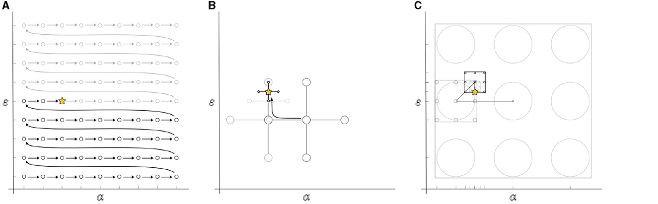
Figure 1. Schematic illustration of the Hyperparameter Optimization (HPO) techniques applied; (A) the exhaustive search method evaluates the entire hyperparameter space, case by case; (B) The direct search method employs a pattern that shrinks in size towards the direction in which the objective function decays; and (C) the recursive search divides the space into subspaces based on the size of the search lattice, shrinking and repositioning the lattice towards the most fitting solution in a recursive manner.
Additionally, we estimated the limits for the lattice-induced deviation of Θmax and Γmax via a second-order Taylor's polynomial approximation (Sauer, 2018), With this strategy, the deviation is obtained with respect to a hypothetical lattice with twice the resolution compared to the actual one.
2.3 Reciprocity principle
The Reciprocity Principle (Fernandez-Corazza et al., 2020) is an explicit approach for obtaining maximum current density, Γmax, based on the reciprocity of the electromagnetic field propagation. Specifically, the maximum stimulation amplitude is obtained with a two-patch tES electrode montage corresponding to the two greatest EEG electrode voltages generated by a desired target current in the brain. The principle considers the connection between the forward and reverse propagation of the electromagnetic field, which is predicted by the lead field matrix.
2.3.1 Formulation of the reciprocity principle for a tES lead field matrix
While gradient propagation in general electromagnetism is not always reciprocal, it can be shown that a bipolar montage in tES corresponds to the greatest absolute back-projected currents in the vector . The reciprocity principle can be formulated, for a restricted system, as
where RK denotes a real N × K (K ≤ N) restriction matrix whose nonzero entries rij, j = 1 correspond to an ordered subset of electrodes
The reciprocity principle follows by writing the intensity as with and describing that Γ can be interpreted as a projection of yK on σKsK. Thus, the maximum of Γ is achieved when yK is parallel to sK. The maximizer is then up-scaled to match the applied current dose μ, i.e., yK = μsK. Therefore, the corresponding maximum intensity is . The optimal maximizer montage is
where, by definition, ||sK||1 = 1 for any K = 1, 2, …, N, and the entries of sK are ordered in descending order with respect to their absolute value. Assuming that these entries are given by λ1 ≥ λ2 ≥ ⋯ ≥ λK ≥ 0, respectively, it holds that , , and
The equality follows a straightforward substitution, the first inequality is based on
and the second one is obtained as . Following from the discriminant, together with the Arithmetic Mean–Quadratic Mean inequality
The second factor in Equation (3) does not have roots if
This assumption is valid since a montage with only two active channels cannot contain more than two halves of the total dose (otherwise, the sum of said currents will be less than zero). Hence, for any montage, and the maximum of Γ is obtained with the bipolar pattern that corresponds to the first two entries i1 and i2 in the set .
2.4 Mathematical optimization software
We solve the optimization task (Equation 2) using the Interior-Point (IP), the Primal-Simplex (PS), and the Dual-Simplex (DS) methods. The class of the IP methods is sub-divided into the primal-dual algorithms (predictor-corrector) (Fiacco and McCormick, 1964; Mehrotra, 1992) and the barrier methods, which determine the feasible set via a barrier function. While IP methods utilize Newton's method to operate in the interior of a feasible set (Boyd and Vandenberghe, 2004), simplex methods seek solutions by considering the feasible set as a convex polytope and moving along its edges. While this strategy uses less memory than the interior-point strategy, it has lower predictability for large-problem convergence.
The concepts of primal- and dual-simplex refer to the formulation of the linear programming problem; by presenting the entries of the current pattern y as differences of non-negative variables (yi = si−pi, si, pi≥0) and the equality constraint via two inequalities (condition a = 0 is satisfied, a ≤ 0 and −a ≤ 0), the task can be brought back to the following standard primal formulation:
whose dual is given by
The IP algorithms applied in this study include Gurobi's parallel barrier method and the primal-dual routines from Matlab, MOSEK, SDPT3, and SeDuMi. The simplex methods include MOSEK's PS and DS, Gurobi's PS and DS, and Matlab's DS algorithm. Matlab's Optimization Toolbox has two IP solvers, of which we apply the interior-point legacy (IPL), whose origin is in the Linear-Programming Interior Point Solvers (LIPSOL) package (Zhang, 1999). All the solvers, their types, and their abbreviations used in this study are described in Table 1.
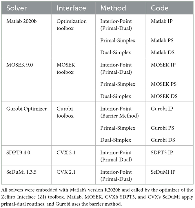
Table 1. Description of the Linear Programming (LP) solvers applied for solving the L1L1 optimization problem through the Interior-Point (IP), Primal-Simplex (PS), and Dual-Simplex (DS) algorithms.
2.5 Numerical domain and computing platform
As the domain of the numerical simulations, we applied a realistic tetrahedral 1.0 mm FE mesh based on an open T1-weighted Magnetic Resonance Imaging (MRI) dataset1. Through FreeSurfer Software Suite2, we segmented the data to find the complex surface boundaries between different tissue compartments, including the skin, skull, cerebrospinal fluid (CSF), gray and white matter, and subcortical structures such as brain stem, thalamus, amygdala, and ventricles (Fischl, 2012). Their conductivity values, which influence the accuracy of the forward solution (Montes-Restrepo et al., 2014), were set according to (Dannhauer et al., 2011). We discretized the volumetric current density to solve the inverse problem using 563 spatial nodes evenly distributed in the gray and white matter compartments of the cerebrum and cerebellum with approximately 1.3 cm (centimeters) distance between two neighboring nodes, associating each node with three divergence-free Cartesian field components.
Through dipole modeling (Bauer et al., 2015; Medani et al., 2015; Pursiainen et al., 2016), we define the region of interests from which the multi-channel tES montage should be derived. We selected the primary somatosensory cortex in the postcentral gyrus (Figure 2A), the primary auditory cortex of the posterior superior temporal gyrus (Figure 2B), and the primary visual cortex in the occipital lobe (Figure 2C) as the target areas. Each dipole is normally oriented with respect to the surface of the gray matter to satisfy the normal constraint of brain activity in the cerebral cortex (Creutzfeldt et al., 1962). Each L1L1 method-based current pattern obtained represents an approximative solution to the optimization problem (Equation 2) corresponding to one of the aforementioned areas.
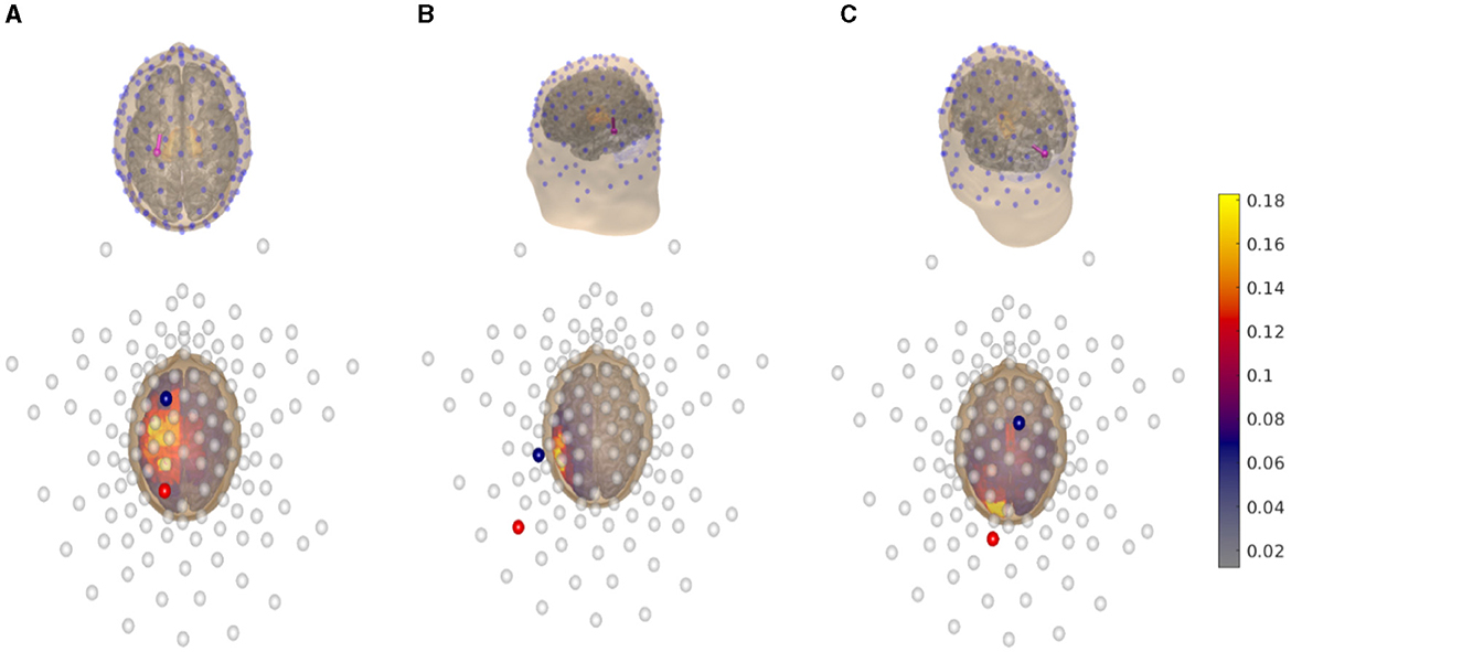
Figure 2. Top row: 3D view of the head model coupled with a 128-channel electrode array (blue dots) following a 10-10 EEG hardware configuration. A synthetic dipole, (magenta spherical arrow), which simulates a current distribution, is placed at the (A) primary somatosensory cortex in the postcentral gyrus, (B) primary auditory cortex in posterior superior temporal gyrus, and (C) primary visual cortex in the occipital lobe, respectively. Bottom row: 2D plane view of the head model displaying the electric field distribution generated by an optimal tES montage following the reciprocity principle which maximizes the focused volumetric current density. The direction of the injection current pattern generated by the montage matches the dipole's orientation. The anodal channels (red spheres) are found by the posterior, while the cathodal channels (blue spheres) by the parietal or frontal sections. The empty circles indicate inactive channels. The volumetric current density is given in Amperes per square meter (A/m2).
We performed the numerical simulations using a Dell 5820 workstation with a 10-core Intel Core i9-10900X processor and 256 GB of RAM. The L1L1 solver was implemented in Matlab-based Zeffiro Interface toolbox3 (He et al., 2019) which builds a high-resolution finite element (FE) mesh and generates a tES lead field matrix (Galaz Prieto et al., 2022) for a given surface-based head segmentation incorporating the Complete Electrode Model's (CEM) boundary conditions (Pursiainen et al., 2012, 2017).
3 Results
The exhaustive search proved to be a reliable method for experimental benchmarking when the required tES montage requires careful design for clinical applications. By presenting the exhaustive search results in the form of a heatmap with a coarse grid of κ = 15 (Figure 3A), we can pinpoint the (α, ε) region where the focused current amplitude reaches its maximum. Despite a significantly increased number of evaluations, with a finer grid of κ = 40 (Figure 3B), we can further determine a more detailed optimal area. This area corresponds to the Cartesian product of αm ranging from −71 to −50 dB and εn from 0 to −98 dB. In this context, a high current injection montage, denoted by Γmax (yellow star), is positioned at the peak of the amplitude, while focality-based montages, Θmax (purple star), adhere closely. However, these focality-based montages are slightly deviated due to the influence of the nuisance field, despite being relatively close, as determined by a threshold condition corresponding to 75% of the maximum amplitude achievable with the two-patch bipolar tES montage. In comparison between these grid resolutions, one can observe slight enhancements in amplitude, increased optimization accuracy, and improved numerical stability in the latter case. These aspects are far more noticeable with Dual- and Primal-Simplex methods than with the Interior-Point, which yields overall smoother results with fewer drastic deviations.
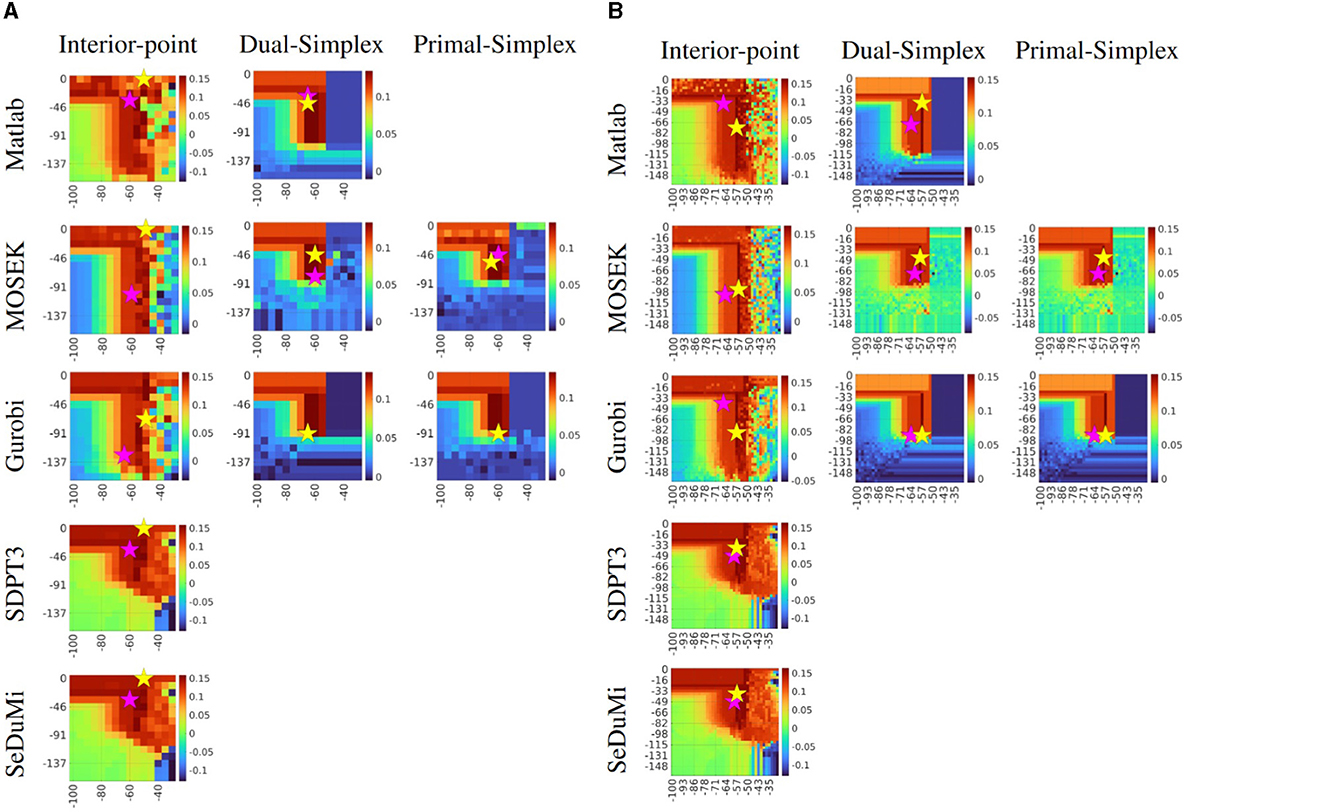
Figure 3. Performance comparison of the exhaustive search for solving the L1-norm fitted and penalized (L1L1) optimization method with current density Γ as the objective function. The coarse (A) search space κ = 15 produces 225 evaluations, and the finer (B) search space κ = 40 with 1600 evaluations, both using regularization parameter α (x-axis) and the nuisance threshold level ε (y-axis). The candidate solutions with respect to current density Γmax and focality Θmax are marked with a yellow and purple star, respectively. The maximizers are generally found around from area in which α is between −71 to −50 dB dB (decibels) and ε from 0 to −98 dB. Notice that in the case of using the Gurobi package, with a Simplex algorithm, both optimal candidate solutions for either a stimulus focality or a current density both optimal solutions are taking the same (α, ε) tuning parameters due to the sharp steepness from the coarse search space. The volumetric current density on every chart is given in Amperes per square meter (A/m2).
Figure 4 delineates the performance nuances among optimization strategies. The whiskers along the stems signify a second-order Taylor's polynomial estimate, reflecting the maximum deviation within half lattice units distance from the optimizer. The reciprocity principle reference for Γmax is represented by a horizontal black dashed line, and the number of non-zero (NNZ) channels required for a tES montage is depicted on the right side of each corresponding stem. The solvers are sorted in ascending order based on their performance, with the exhaustive search κ = 40 grid (blue) serving as the point of reference. Both the direct and recursive search techniques adeptly uncover optimal (α, ε) solutions for Θmax and Γmax, yielding a substantial reduction in total computing time compared to the specified hyperparameter space.
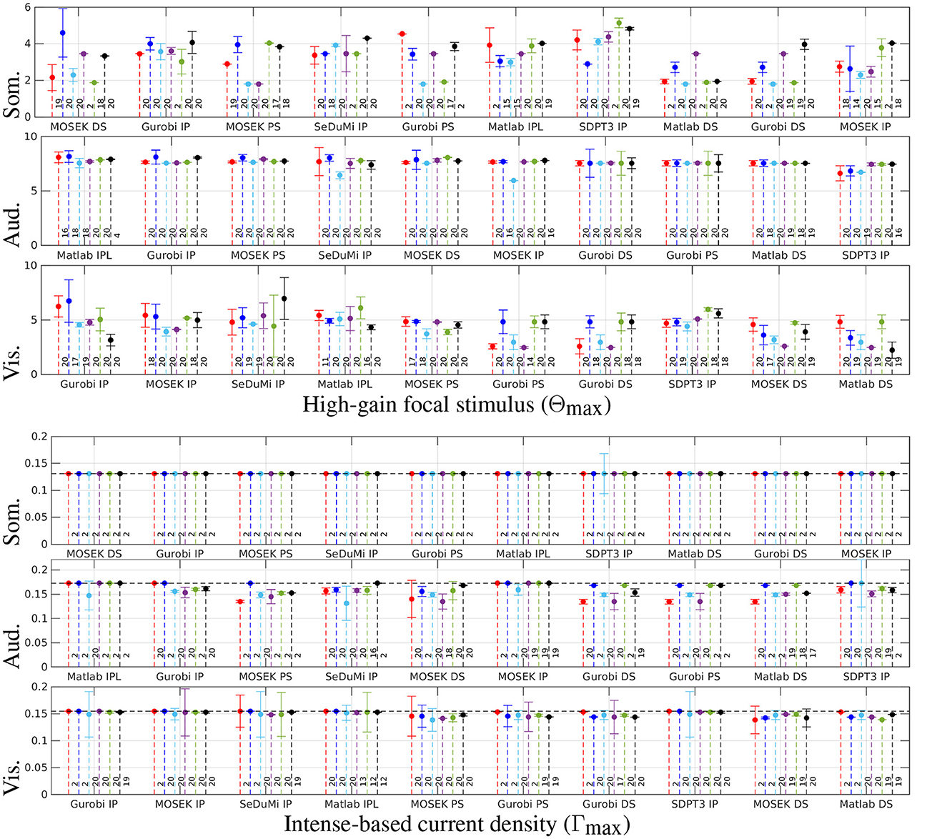
Figure 4. Stem plots results from the two-stage metaheuristic lattice search using exhaustive search with coarse grid of κ = 15 (red) and fine grid of κ = 40 (blue), and a recursive one with (cyan, magenta, green, and black, respectively) considering the somatosensory (Som.), auditory (Aud.) and visual (Vis.) regions of interest. The whiskers in the stem plot indicate a second-order Taylor's polynomial estimate for the maximum deviation within a half-lattice unit distance from the optimizer. The intense current injection (Γmax) calculated using the reciprocity principle is shown with a horizontal black dashed line as a reference. The number of non-zero (NNZ) channels in the Transcranial Electrical Stimulation (tES) montage is shown on the right side next to the corresponding stem. The solvers are sorted in descending order from left to right based on their performance with κ = 40.
Due to the heuristic nature of the direct search, and to assert the efficacy of the said technique, we performed a series of trial runs by setting the initial point to the center of the search space. In these trials, the number of objective function evaluations varied, ranging from 25 to 54 trials, with a 33.8 mean among the evaluations (see Table 2). While the number of function evaluations was slightly higher, the quality of the results was nearly on par with those obtained with the recursive search with a search window of . With IP solvers, the search runs were mostly successful, while PS and DS tended to fail to find a feasible optimizer candidate.
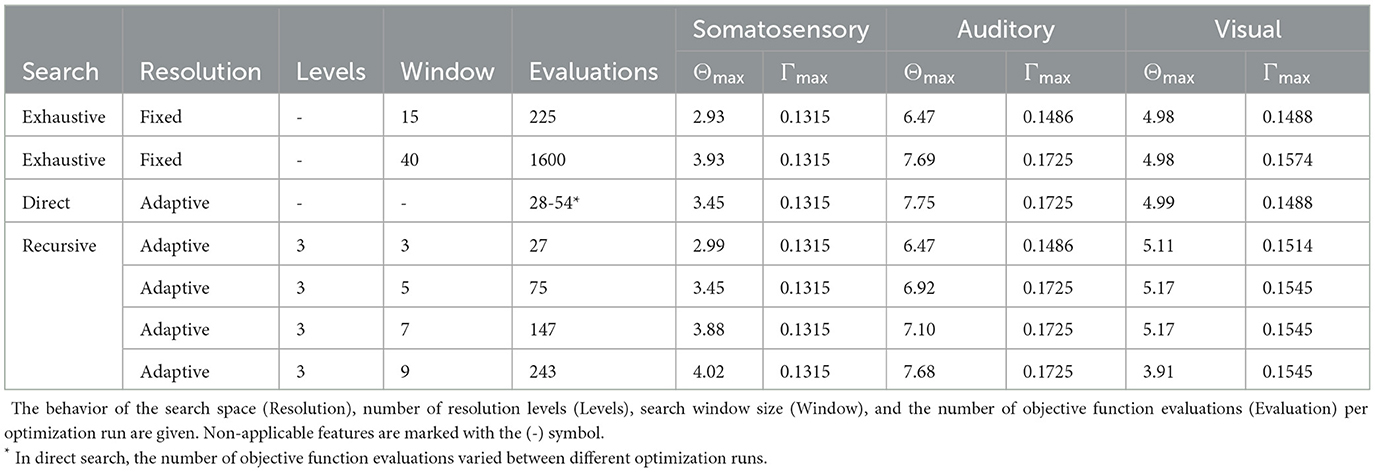
Table 2. Comparison of stimulation focality Θmax and intensity Γmax results obtained between exhaustive, direct, and recursive search methods.
Due to its relatively fast performance among interior-point methods, we applied MOSEK IP to evaluate topographical maps of stimulus focality Θmax (Figure 5A) and current density Γmax (Figure 5B) for an exhaustive search κ = 15 and a recursive search . Overall, the results of the recursion were close to the outcome of the exhaustive search. Thus, the topographical differences between the different approaches of this study were observed to be minor.
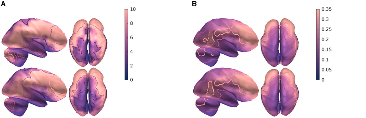
Figure 5. Comparison of the topographical maps for (A) maximum focality Θmax and (B) current density Γmax using exhaustive search κ = 15 (top-row), and recursion with (bottom-row). The contours show 20, 40, and 75% equicurves with respect to their maximum entry. Maps have been computed using the MOSEK with the Interior-point method.
By limiting the search space only to a narrower subspace is a simple countermeasure for dealing with the disadvantages of the exhaustive search. With a κ = 15 grid as a reference, it can take approximately 850 seconds to perform a complete search for the first stage, while the second stage only takes roughly 15% of that time since it uses a limited lead field following from the limited number of active electrodes. As an alternative approach, the direct and recursive search seemed to perform well compared to the number of objective function evaluations made during the search process (Figure 6). In particular, MOSEK turned out to be the superior choice, with MOSEK DS being the fastest one. The computing time for Gurobi IP was close to that of MOSEK IP, and Gurobi DS, PS, and Matlab IPL and DS required approximately three times the time. The slowest-performing SDPT3 and SeDuMi took as much as six times the run time of MOSEK IP. Overall, the simplex methods applied to the L1L1 optimization scheme deliver faster yet less accurate solutions than Interior-Point (IP) for focality-based montages, while minor differences can be found for intensity-based solutions.
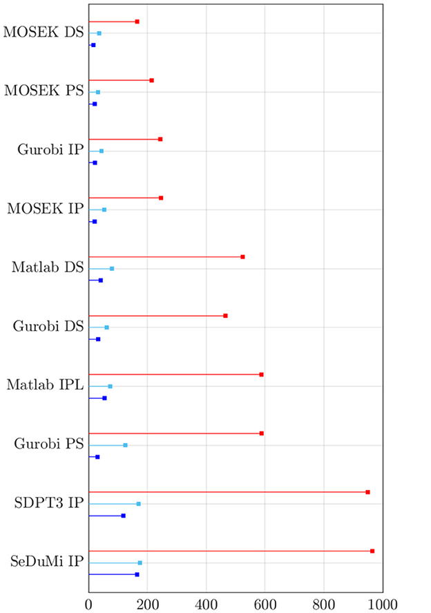
Figure 6. Total amount of computing time for finding the most fitting candidate solution through the two-stage metaheuristic lattice search on every optimization solver and method in this study. In order of stem (top-to-bottom): exhaustive search with search space κ = 15 (red), direct search (cyan), and recursive search with (blue). Noticeably, the non-commercial solvers from CVX (SDPT3 and SeDuMi) are significantly slower than those produced by Matlab, Gurobi and MOSEK.
4 Discussion
In this study, we analyzed the numerical and computational performance of exhaustive search, direct search, and recursive search techniques to find an optimal stimulation focality Θ and current density Γ for solving the L1L1 optimization problem for non-invasive transcranial electrical stimulation (tES) current injection. This analysis was motivated by our earlier results in (Galaz Prieto et al., 2022) which suggested that the L1L1 method provides a theoretically attractive approach for obtaining a high-gain focal stimulus as compared to complex L2-norm fitting and regularized least squares techniques (Dmochowski et al., 2011; Wagner et al., 2016).
The reciprocity principle, as outlined by Fernandez-Corazza et al. (2020), served as a reference technique. Its validity was shown for the present tES lead field matrix L (see Section 2.3.1). When focusing on a specific target region, the current injection pattern from a two-patch tES montage aligns with the maximum intensity achievable through this principle. Essentially, this involves selecting the two electrodes with the highest absolute back-projected currents. With the absence of nuisance field constraints, the L1L1 solution was observed to agree with the reciprocity principle if the aforementioned algorithmic aspects were handled appropriately.
Decisive aspects for a successful outcome of L1L1 were found to be the choice of the optimization package, algorithm, and search routine, which significantly affect both the performance of the metaheuristic optimization process and output. To enlighten this aspect, we covered the performance of several Interior-Point (IP) (Mehrotra, 1992), Dual-Simplex (DS), and Primal-Simplex (PS) (Boyd and Vandenberghe, 2004) methods from different open-source and commercial optimization toolboxes. We tested the L1L1 method using the commercial solvers of MOSEK Optimization Suite (Release 9) (Mosek, 2019) and Gurobi Optimization (9.5.1) (Gurobi Optimization LLC, 2022), and compared them to the open-source alternatives (Grant and Boyd, 2014) SDPT3 (4.0) (Tütüncü et al., 2003) and SeDuMi (1.3.5) (Sturm, 1999; Frenk et al., 2000; Polik et al., 2007) as well as Matlab R2020b's (MathWorks) Interior-Point-Legacy (IPL) algorithm, which originates from the open LIPSOL (Zhang, 1999) toolbox. We selected the IPL algorithm since we experienced stagnation with Matlab's main IP algorithm, which did not return any appropriate results.
Based on the results, we consider Gurobi IP to be the preferable choice in both optimization stages, considering Θmax and Γmax in each tested target region of interest and, as it was also overall the fastest of the IP solvers. While the best-performing solvers show that the L1L1 method is suitable for maximizing focality and intensity, a few did not find the bipolar current pattern that maximizes Γmax. Notably, SDTP3 did not find a bipolar pattern at all, verifying our earlier hypothesis (Galaz Prieto et al., 2022) that the performance of L1L1 might be highly solver-based. Part of the discrepancies between the optimization methods can be explained by a different sensitivity with respect to parameter variation or the resolution of the lattice.
From a computational complexity standpoint, the exhaustive search method can be applied for benchmarking purposes. In contrast, a recursive search proves an advantageous alternative and is competitively on par with the direct search technique, each one applied in this study. This equivalence arises from both methods converging toward the most suitable regularization parameter α and nuisance threshold ε values in a comparably controlled manner. Notably, the computational complexity of recursive search remains consistent across various optimization runs, in contrast to the variability observed in the direct search. Results comparable to those obtained through exhaustive search can be attained with a reduced-resolution search window of, say, size , representing a substantial acceleration in comparison to exhaustive search. Furthermore, the recursive approach demonstrates both numerical stability and convergence towards exhaustive search results, both at individual data points and in the overall topographical context, as the probing lattice size increases.
4.1 Limitations and future work
Unlike earlier linear programming (LP) formulations for tES optimization problems, our use of the metaheuristic process enabled us to explore parameters freely, without imposing rigid a priori constraints on the nuisance field, as observed in Wagner et al. (2016). In L1L1, we optimally set the nuisance field through hyperparameter optimization embedded in a two-stage metaheuristic lattice search procedure. Interpreted as an enhancement for localizing both pattern and volumetric density of the stimulus, L1-norm fitting and regularization outperform the least-squares methodology introduced in Dmochowski et al. (2011, 2017). However, this improvement comes at a greater computational cost, prompting our in-depth investigation into various algorithmic aspects of metaheuristic optimization in this study. Our present findings underscore the critical role of computational considerations when integrating hyperparameters and metacriteria into the tES optimization problem, aspects overlooked in the studies mentioned earlier.
Our results concerning L1L1 are limited to numerically simulated tES only, meaning that neither the performance of the method in other modalities than tES nor the effects of uncertainty causing inter-subject variability (Laakso et al., 2015) have not been fully covered yet. Those might include, for example, any discrepancies between the estimated and actual values of electrical conductivity, such as skull conductivity (Schmidt et al., 2015), strategy to specify a montage (Kaufmann et al., 2021), as well as uncertainty about the targeted region in the brain, e.g., a possible spread of an epileptic focus (Simula et al., 2022). While the expected level of uncertainty can be controlled via the range of the hyperparameter ε, a future study on its effect will obviously need to be conducted.
Of the applied liner programming methods, interior-point is an overall preferable option over the simplex methods, which can be considered beneficial characteristic when hardware performance is limited, e.g., for a potential Field-Programmable Gate Array (FPGA) implementation (Bayliss et al., 2006; Gensheimer et al., 2014). Another comparative method, the Alternating Direction Method of Multipliers (ADMM) (Lin et al., 2021), was not included in this investigation as achieving an appropriate convergence seemed more difficult due to its dependence on a step-length parameter. While the current results enlighten how the different algorithms would perform with different nuisance threshold levels, an independent study would be needed to determine the optimal level given the mathematical uncertainty.
Possible future work directions can be to open up the function of L1L1 on a broader scale, this include applying it for deep brain stimulation (DBS), where the electrical stimulus is not transcranial. Likewise, an advanced optimization technique is needed to target subcortical nuclei of the brain; for instance, in the recent study (Anderson et al., 2018), where the Interior-Point algorithm has been applied. Yet another interesting direction is to consider a priori information for the design and application of the L1L1 algorithm, for example, an epileptic focus based on non-invasive measurements such as video-EEG of epileptic activity applied to determine approximate stimulation locations. Finally, the mathematical implications of this study can be further enriched by incorporating transcranial direct current stimulation and functional magnetic resonance imaging (tDCS-fMRI) (Esmaeilpour et al., 2020). By utilizing tDCS-fMRI data sets to explore real-time neural changes caused by electrical stimulation–such as in the studies by Callan et al. (2016) for investigating resting state networks linked to visual stimuli, or in the research conducted by Mark et al. (2023) for monitoring brain activity of pilots undergoing aviation training–further enriches the necessity of an effective inverse problem study equipped with optimization methods for simulating and understanding the signal-to-noise (SNR) impacts with a level of mathematical uncertainty, as some of these deficiencies were mentioned on their study limitations.
Data availability statement
The original contributions presented in the study are included in the article/supplementary material, further inquiries can be directed to the corresponding author.
Author contributions
FG: Conceptualization, Data curation, Formal analysis, Investigation, Methodology, Software, Visualization, Writing—original draft. MS: Formal analysis, Project administration, Supervision, Validation, Software, Visualization, Writing—original draft, Writing—review & editing. SP: Conceptualization, Data curation, Formal analysis, Funding acquisition, Investigation, Methodology, Project administration, Resources, Software, Supervision, Validation, Visualization, Writing—review & editing.
Funding
FG, MS, and SP were supported by the Research Council of Finland through the Center of Excellence in Inverse Modelling and Imaging 2018–2025 (decision 353089), the researcher exchange (DAAD) project “Non-invasively reconstructing and inhibiting activity in focal epilepsy” (decision 354976), the ERA PerEpi project (decision 344712), and Flagship of Advanced Mathematics for Sensing, Imaging and Modelling (decision 359185).
Acknowledgments
The authors would like to thank Prof. Dr. rer. nat. Carsten Wolters, researchers and clinicians from the Institute for Biomagnetism and Biosignalanalysis (IBB), and the PerEpi consortium for their continuous support, discussions, and feedback regarding non-invasive brain stimulation topics, regression analysis, and the seminars prepared during the elaboration of this study.
Conflict of interest
The authors declare that the research was conducted in the absence of any commercial or financial relationships that could be construed as a potential conflict of interest.
Publisher's note
All claims expressed in this article are solely those of the authors and do not necessarily represent those of their affiliated organizations, or those of the publisher, the editors and the reviewers. Any product that may be evaluated in this article, or claim that may be made by its manufacturer, is not guaranteed or endorsed by the publisher.
Footnotes
References
Anderson, D. N., Osting, B., Vorwerk, J., Dorval, A. D., and Butson, C. R. (2018). Optimized programming algorithm for cylindrical and directional deep brain stimulation electrodes. J. Neural Eng. 15, 026005. doi: 10.1088/1741-2552/aaa14b
Bauer, M., Pursiainen, S., Vorwerk, J., Köstler, H., and Wolters, C. H. (2015). Comparison study for Whitney (Raviart-Thomas) type source models in finite element method based EEG forward modeling. IEEE Trans. Biomed. Eng. 62, 2648–2656. doi: 10.1109/TBME.2015.2439282
Bayliss, S., Constantinides, G. A., Luk, W., et al. (2006). “An FPGA implementation of the simplex algorithm,” in 2006 IEEE International Conference on Field Programmable Technology (Bangkok: IEEE), 49–56.
Bianchi, L., Dorigo, M., Gambardella, L. M., and Gutjahr, W. J. (2009). A survey on metaheuristics for stochastic combinatorial optimization. Nat. Comput. 8, 239–287. doi: 10.1007/s11047-008-9098-4
Bogani, C., Gasparo, M., and Papini, A. (2009). Generalized pattern search methods for a class of nonsmooth optimization problems with structure. J. Comput. Appl. Math. 229, 283–293. doi: 10.1016/j.cam.2008.10.047
Callan, D. E., Falcone, B., Wada, A., and Parasuraman, R. (2016). Simultaneous tdcs-fMRI identifies resting state networks correlated with visual search enhancement. Front. Hum. Neurosci. 10, 72. doi: 10.3389/fnhum.2016.00072
Creutzfeldt, O. D., Fromm, G. H., and Kapp, H. (1962). Influence of transcortical dc currents on cortical neuronal activity. Exp. Neurol. 5, 436–452. doi: 10.1016/0014-4886(62)90056-0
Dannhauer, M., Lanfer, B., Wolters, C. H., and Knösche, T. R. (2011). Modeling of the human skull in EEG source analysis. Hum. Brain Mapp. 32, 1383–1399. doi: 10.1002/hbm.21114
Dmochowski, J. P., Datta, A., Bikson, M., Su, Y., and Parra, L. C. (2011). Optimized multi-electrode stimulation increases focality and intensity at target. J. Neural Eng. 8, 046011. doi: 10.1088/1741-2560/8/4/046011
Dmochowski, J. P., Koessler, L., Norcia, A. M., Bikson, M., and Parra, L. C. (2017). Optimal use of eeg recordings to target active brain areas with transcranial electrical stimulation. Neuroimage 157, 69–80. doi: 10.1016/j.neuroimage.2017.05.059
Esmaeilpour, Z., Shereen, A. D., Ghobadi-Azbari, P., Datta, A., Woods, A. J., Ironside, M., et al. (2020). Methodology for tdcs integration with fmri. Hum. Brain Mapp. 41, 1950–1967. doi: 10.1002/hbm.24908
Faria, P., Hallett, M., and Miranda, P. C. (2011). A finite element analysis of the effect of electrode area and inter-electrode distance on the spatial distribution of the current density in tdcs. J. Neural Eng. 8, 066017. doi: 10.1088/1741-2560/8/6/066017
Fernandez-Corazza, M., Turovets, S., and Muravchik, C. H. (2020). Unification of optimal targeting methods in transcranial electrical stimulation. Neuroimage 209, 116403. doi: 10.1016/j.neuroimage.2019.116403
Feurer, M., and Hutter, F. (2019). “Hyperparameter optimization,” in Automated Machine Learning. (Cham: Springer), 3–33.
Fiacco, A. V., and McCormick, G. P. (1964). The sequential unconstrained minimization technique for nonlinear programing, a primal-dual method. Manage. Sci. 10:360–366. doi: 10.1287/mnsc.10.2.360
Frenk, H., Roos, K., Terlaky, T., and Zhang, S. (2000). “Central region method,” in High Performance Optimization, 157–194.
Galaz Prieto, F., Rezaei, A., Samavaki, M., and Pursiainen, S. (2022). L1-norm vs. l2-norm fitting in optimizing focal multi-channel tes stimulation: linear and semidefinite programming vs. weighted least squares. Comput. Methods Programs Biomed. 226:107084. doi: 10.1016/j.cmpb.2022.107084
Gensheimer, F., Ruzika, S., Scholl, S., and Wehn, N. (2014). “A simplex algorithm for lp decoding hardware,” in 2014 IEEE 25th Annual International Symposium on Personal, Indoor, and Mobile Radio Communication (PIMRC) (Washington, DC: IEEE), 790–794
Grant, M., and Boyd, S. (2014). CVX: Matlab Software for Disciplined Convex Programming, Version 2.1. Available online at: http://cvxr.com/cvx
Guler, S., Dannhauer, M., Erem, B., Macleod, R., Tucker, D., Turovets, S., et al. (2016). Optimization of focality and direction in dense electrode array transcranial direct current stimulation (tdcs). J. Neural Eng. 13, 036020. doi: 10.1088/1741-2560/13/3/036020
Gurobi Optimization LLC (2022). Gurobi Optimizer Reference Manual. Available online at: https://www.gurobi.com
He, Q., Rezaei, A., and Pursiainen, S. (2019). Zeffiro user interface for electromagnetic brain imaging: A gpu accelerated fem tool for forward and inverse computations in matlab. Neuroinformatics 18, 237–250. doi: 10.1007/s12021-019-09436-9
Je, C., and Park, H.-M. (2013). Optimized hierarchical block matching for fast and accurate image registration. Signal Proc. Image Commun. 28, 779–791. doi: 10.1016/j.image.2013.04.002
Kaufmann, E., Hordt, M., Lauseker, M., Palm, U., and Noachtar, S. (2021). Acute effects of spaced cathodal transcranial direct current stimulation in drug resistant focal epilepsies. Clini, Neurophysiol, 132, 1444–1451. doi: 10.1016/j.clinph.2021.03.048
Khadka, N., Borges, H., Paneri, B., Kaufman, T., Nassis, E., Zannou, A. L., et al. (2020). Adaptive current tdcs up to 4ma. Brain Stimul. 13, 69–79. doi: 10.1016/j.brs.2019.07.027
Khan, A., Antonakakis, M., Vogenauer, N., Haueisen, J., and Wolters, C. H. (2022). Individually optimized multi-channel tdcs for targeting somatosensory cortex. Clini. Neurophysiol. 134, 9–26. doi: 10.1016/j.clinph.2021.10.016
Kowalski, T., Silny, J., and Buchner, H. (2002). Current density threshold for the stimulation of neurons in the motor cortex area. Bioelectromagnetics. 23, 421–428. doi: 10.1002/bem.10036
Laakso, I., Tanaka, S., Koyama, S., De Santis, V., and Hirata, A. (2015). Inter-subject variability in electric fields of motor cortical tdcs. Brain Stimul. 8, 906–913. doi: 10.1016/j.brs.2015.05.002
Lin, T., Ma, S., Ye, Y., and Zhang, S. (2021). An admm-based interior-point method for large-scale linear programming. Optimizat. Methods Softw. 36, 389–424. doi: 10.1080/10556788.2020.1821200
Mark, J. A., Ayaz, H., and Callan, D. E. (2023). Simultaneous fmri and tdcs for enhancing training of flight tasks. Brain Sci. 13, 1024. doi: 10.3390/brainsci13071024
Medani, T., Lautru, D., Ren, Z., Schwartz, D., and Sou, G. (2015). “Modelling of brain sources using the modified saint Venant's method in FEM resolution of EEG forward problem,” in Conference IEEE EMBS Conference on Neural Engineering 2015, 7th International IEEE EMBS Conference on Neural Engineering (Montpellier, France: IEEE).
Mehrotra, S. (1992). On the implementation of a primal-dual interior point method. SIAM J. Optimizat. 2, 575–601. doi: 10.1137/0802028
Montes-Restrepo, V., Van Mierlo, P., Strobbe, G., Staelens, S., Vandenberghe, S., and Hallez, H. (2014). Influence of skull modeling approaches on eeg source localization. Brain Topogr. 27, 95–111. doi: 10.1007/s10548-013-0313-y
Moreno-Duarte, I., Gebodh, N., Schestatsky, P., Guleyupoglu, B., Reato, D., Bikson, M., et al. (2014). “Chapter 2-transcranial electrical stimulation: Transcranial direct current stimulation (tdcs), transcranial alternating current stimulation (tacs), transcranial pulsed current stimulation (tpcs), and transcranial random noise stimulation (trns),” in The Stimulated Brain, R. Cohen Kadosh (San Diego: Academic Press), 35–59.
MOSEK ApS (2019). Mosek Optimization Toolbox for Matlab. Users Guide and Reference Manual, Version. MOSEK, 4, 1.
Nitsche, M. A., and Paulus, W. (2000). Excitability changes induced in the human motor cortex by weak transcranial direct current stimulation. J. Physiol. 527, 633–639. doi: 10.1111/j.1469-7793.2000.t01-1-00633.x
Paulus, W. (2011). Transcranial electrical stimulation (tes - tdcs; trns, tacs) methods. Neuropsychol. Rehabil. 21, 602–617. doi: 10.1080/09602011.2011.557292
Peterchev, A. V., Wagner, T. A., Miranda, P. C., Nitsche, M. A., Paulus, W., Lisanby, S. H., et al. (2012). Fundamentals of transcranial electric and magnetic stimulation dose: Definition, selection, and reporting practices. Brain Stimul. 5, 435–453. doi: 10.1016/j.brs.2011.10.001
Polik, I., Terlaky, T., and Zinchenko, Y. (2007). “Sedumi: a package for conic optimization,” in IMA Workshop on Optimization and Control, Univ. Minnesota, Minneapolis. Minnesota, Minneapolis: Citeseer.
Pursiainen, S., Agsten, B., Wagner, S., and Wolters, C. H. (2017). Advanced boundary electrode modeling for tes and parallel tes/eeg. IEEE Trans. Neural Syst. Rehabilitat. Eng. 26, 37–44. doi: 10.1109/TNSRE.2017.2748930
Pursiainen, S., Lucka, F., and Wolters, C. H. (2012). Complete electrode model in EEG: relationship and differences to the point electrode model. Phys. Med. Biol., 57, 999–1017. doi: 10.1088/0031-9155/57/4/999
Pursiainen, S., Vorwerk, J., and Wolters, C. H. (2016). Electroencephalography (EEG) forward modeling viaH(div) finite element sources with focal interpolation. Phys. Med. Biol. 61, 8502–8520. doi: 10.1088/0031-9155/61/24/8502
Rampersad, S., Stegeman, D., and Oostendorp, T. (2013). Op 11 optimized tdcs electrode configurations for five targets determined via an inverse fe modeling approach. Clini. Neurophysiol. 124, e61–e62. doi: 10.1016/j.clinph.2013.04.078
Reed, T., and Cohen Kadosh, R. (2018). Transcranial electrical stimulation (tes) mechanisms and its effects on cortical excitability and connectivity. J. Inherit. Metab. Dis. 41, 1123–1130. doi: 10.1007/s10545-018-0181-4
Roy, A., Boroda, E., Waldron, E., Lim, K., and Henry, T. (2019). Integration of prefrontal transcranial direct current stimulation with cognitive training for treatment of memory dysfunction in epilepsy. Brain Stimulat. 12, 481. doi: 10.1016/j.brs.2018.12.571
Ruffini, G., Fox, M. D., Ripolles, O., Miranda, P. C., and Pascual-Leone, A. (2014). Optimization of multifocal transcranial current stimulation for weighted cortical pattern targeting from realistic modeling of electric fields. Neuroimage 89, 216–225. doi: 10.1016/j.neuroimage.2013.12.002
Schmidt, C., Wagner, S., Burger, M., van Rienen, U., and Wolters, C. H. (2015). Impact of uncertain head tissue conductivity in the optimization of transcranial direct current stimulation for an auditory target. J. Neural Eng. 12, 046028. doi: 10.1088/1741-2560/12/4/046028
Simula, S., Daoud, M., Ruffini, G., Biagi, M. C., Bénar, C.-G., Benquet, P., et al. (2022). Transcranial current stimulation in epilepsy: a systematic review of the fundamental and clinical aspects. Front. Neurosci. 16, 909421. doi: 10.3389/fnins.2022.909421
Sturm, J. F. (1999). Using sedumi 1.02, a matlab toolbox for optimization over symmetric cones. Optimization methods and software 11:625–653. doi: 10.1080/10556789908805766
Thair, H., Holloway, A. L., Newport, R., and Smith, A. D. (2017). Transcranial direct current stimulation (tdcs): A beginner's guide for design and implementation. Front. Neurosci. 11, 641. doi: 10.3389/fnins.2017.00641
Tost, A., Migliorelli, C., Bachiller, A., Medina-Rivera, I., Romero, S., García-Cazorla, Á., et al. (2021). Choosing strategies to deal with artifactual eeg data in children with cognitive impairment. Entropy 23, 1030. doi: 10.3390/e23081030
Tütüncü, R. H., Toh, K.-C., and Todd, M. J. (2003). Solving semidefinite-quadratic-linear programs using sdpt3. Mathemat. Program. 95, 189–217. doi: 10.1007/s10107-002-0347-5
Wagner, S., Burger, M., and Wolters, C. H. (2016). An optimization approach for well-targeted transcranial direct current stimulation. SIAM J. Appl. Math. 76, 2154–2174. doi: 10.1137/15M1026481
Wagner, S., Rampersad, S. M., Aydin, U., Vorwerk, J., Oostendorp, T. F., Neuling, T., et al. (2013). Investigation of tdcs volume conduction effects in a highly realistic head model. J. Neural Eng. 11, 016002. doi: 10.1088/1741-2560/11/1/016002
Workman, C. D., Fietsam, A. C., and Rudroff, T. (2020). Different effects of 2 ma and 4 ma transcranial direct current stimulation on muscle activity and torque in a maximal isokinetic fatigue task. Front. Hum. Neurosci. 14, 240. doi: 10.3389/fnhum.2020.00240
Yang, L., and Shami, A. (2020). On hyperparameter optimization of machine learning algorithms: Theory and practice. Neurocomputing 415, 295–316. doi: 10.1016/j.neucom.2020.07.061
Zaghi, S., Acar, M., Hultgren, B., Boggio, P. S., and Fregni, F. (2010). Noninvasive brain stimulation with low-intensity electrical currents: Putative mechanisms of action for direct and alternating current stimulation. Neuroscientist 16, 285–307. doi: 10.1177/1073858409336227
Keywords: transcranial electrical stimulation (tES), optimization, linear programming, L1-norm, Interior-Point, metaheuristics
Citation: Galaz Prieto F, Samavaki M and Pursiainen S (2024) Lattice layout and optimizer effect analysis for generating optimal transcranial electrical stimulation (tES) montages through the metaheuristic L1L1 method. Front. Hum. Neurosci. 18:1201574. doi: 10.3389/fnhum.2024.1201574
Received: 06 April 2023; Accepted: 16 February 2024;
Published: 29 February 2024.
Edited by:
Kanak Kalita, Vel Tech Dr. RR & Dr. SR Technical University, IndiaReviewed by:
Umit Aydin, University of Reading, United KingdomGhazaleh Soleimani, Medical School, University of Minnesota, United States
Copyright © 2024 Galaz Prieto, Samavaki and Pursiainen. This is an open-access article distributed under the terms of the Creative Commons Attribution License (CC BY). The use, distribution or reproduction in other forums is permitted, provided the original author(s) and the copyright owner(s) are credited and that the original publication in this journal is cited, in accordance with accepted academic practice. No use, distribution or reproduction is permitted which does not comply with these terms.
*Correspondence: Fernando Galaz Prieto, ZmVybmFuZG8uZ2FsYXpwcmlldG9AdHVuaS5maQ==