 Tsuneo Nitta
 Junsei Horikawa1
 Yurie Iribe
 Ryo Taguchi
 Shuji Shinohara
 Goh Kawai
95% of researchers rate our articles as excellent or good
Learn more about the work of our research integrity team to safeguard the quality of each article we publish.
Find out more
ORIGINAL RESEARCH article
Front. Hum. Neurosci. , 18 May 2023
Sec. Brain-Computer Interfaces
Volume 17 - 2023 | https://doi.org/10.3389/fnhum.2023.1163578
This article is part of the Research Topic Neural Decoding for Direct Communication in Brain-Computer Interface View all 6 articles
Speech imagery recognition from electroencephalograms (EEGs) could potentially become a strong contender among non-invasive brain-computer interfaces (BCIs). In this report, first we extract language representations as the difference of line-spectra of phones by statistically analyzing many EEG signals from the Broca area. Then we extract vowels by using iterative search from hand-labeled short-syllable data. The iterative search process consists of principal component analysis (PCA) that visualizes linguistic representation of vowels through eigen-vectors φ(m), and subspace method (SM) that searches an optimum line-spectrum for redesigning φ(m). The extracted linguistic representation of Japanese vowels /i/ /e/ /a/ /o/ /u/ shows 2 distinguished spectral peaks (P1, P2) in the upper frequency range. The 5 vowels are aligned on the P1-P2 chart. A 5-vowel recognition experiment using a data set of 5 subjects and a convolutional neural network (CNN) classifier gave a mean accuracy rate of 72.6%.
In the field of neural decoding for direct communication in brain-computer interfaces (BCIs), research is progressing for detecting spoken signals from multi-channel electrocorticograms (ECoGs) at the brain cortex (Knight and Heinze, 2008; Pasley et al., 2012; Bouchard et al., 2013; Flinker et al., 2015; Herff and Schultz, 2016; Martin et al., 2018; Anumanchipalli et al., 2019; Miller et al., 2020). If we could instead detect linguistic information from scalp EEGs, then BCIs could enjoy much wider practical applications, for instance improving the quality of life (QoL) of amyotrophic lateral sclerosis (ALS) patients, but this goal is hampered by many unsolved problems (Wang et al., 2012; Min et al., 2016; Rojas and Ramos, 2016; Yoshimura et al., 2016; Yu and Shafer, 2021; Zhao et al., 2021). While studies on spoken EEGs can leverage motor command information to help identify speech-related signals, imagined speech EEGs (that is, EEGs of silent, unspoken speech) lack that luxury (Levelt, 1993; Indefrey and Levelt, 2004), which necessitates identifying linguistic representations solely from within the EEG.
Linear predictive coding (LPC) is the widely used international standard for speech coding (Itakura and Saito, 1968; Ramirez, 2008). The LPC takes an analysis by synthesis (AbS) approach. The authors believe that EEG signal analysis would similarly benefit from linear predictive analysis (LPA) that incorporates brain wave production models (see the section “2. Materials and methods”).
Speech recognition technology was propelled by phone-labeled speech corpora such as those distributed by the Linguistic Data Consortium (LDC).1 Speech imagery recognition technology also needs speech corpora labeled at the phone or syllable levels. The authors used a pooling process to combine multi-electrode spectra, and manually identified and labeled chunks of discrete consonant-vowel (CV) monosyllables found in the EEG signals (see section “2. Materials and methods”).
EEG signals differ from speech signals in that unlike spoken speech, EEG signals do not exhibit coarticulation. Instead, sequences of discrete monosyllables 50 to 80 [ms] in duration are found. In the section “2. Materials and Methods,” Figure 7 shows an example of EEG spectrum of connected imagined speech, where CV are observed with no coarticulation. Coarticulation occurs at the muscular motor phase of speech production, where the movements of vocal organs effectively slur into each other.
In our vowel classification experiment involving 5 male and 1 female human subjects, we saw no marked difference of EEG signals with respect to the speaker’s sex or age. We intend to verify this in future studies by collecting more EEG data and classifying vowels. At this time, however, we attempted subject-independent recognition of the 5 vowels in Japanese language by using linguistic representations of vowels as input to the CNN.
This section discusses extracting and evaluating linguistic representation of vowels (Figure 1).
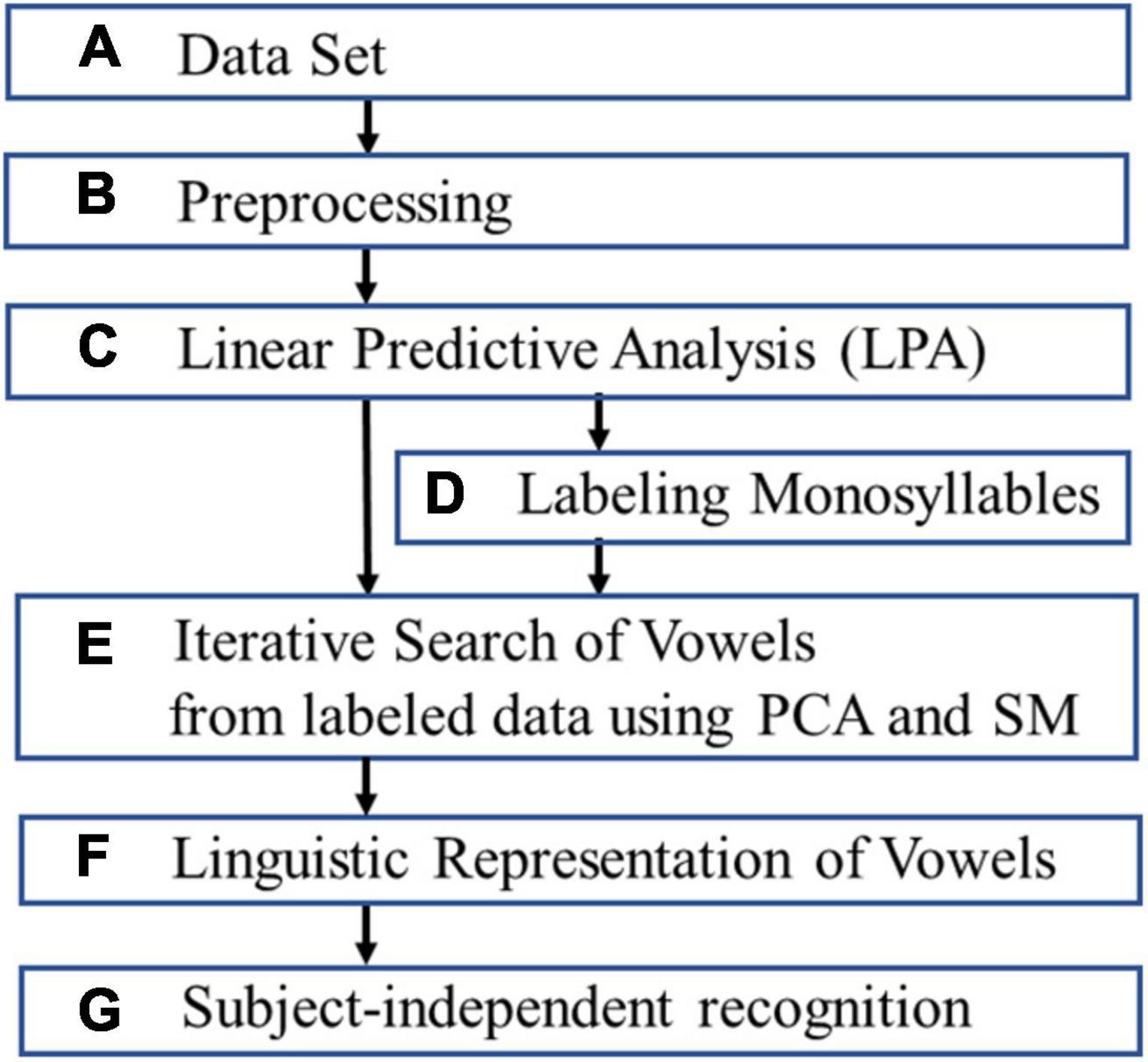
Figure 1. The flow chart for extracting and evaluating linguistic representation of vowels.
We recorded scalp EEG signals using model g.HIAMP manufactured by g.tec (g.tec medical engineering, Graz, Austria). Measurements were taken in a sound-proof and electromagnetic interference (EMI)-proof chamber at Aichi Prefectural University (APU). Figure 2 shows the placement of 21 electrodes in the extended international 10–20 system using the modified combinatorial nomenclature (MCN). The electrodes shown in green were used to measure EEG in our experiment.
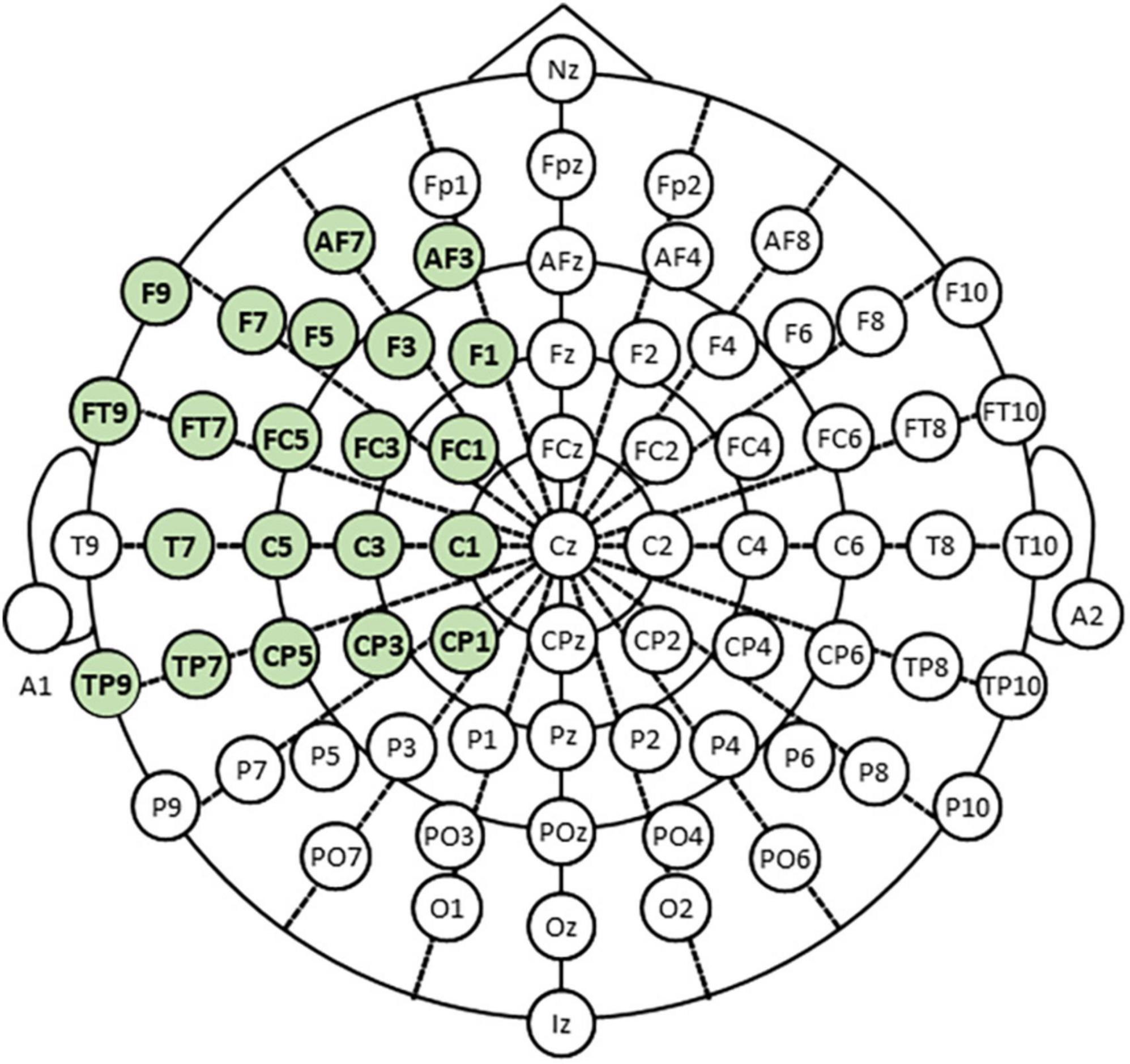
Figure 2. Electroencephalogram (EEG) electrode positions shown in the extended 10–20 system.
The human subjects were 1 female [F1, 23 years old (y.o.)] and 4 males (M1, M2, M3, M4, 23, 22, 22, 74 y.o, respectively), all with normal hearing and right-handed. Written informed consent was obtained from all subjects prior to data collection. The experimental protocol was approved by the APU ethics committee.
Table 1 shows the imagined speech data set of 57 Japanese short syllables.
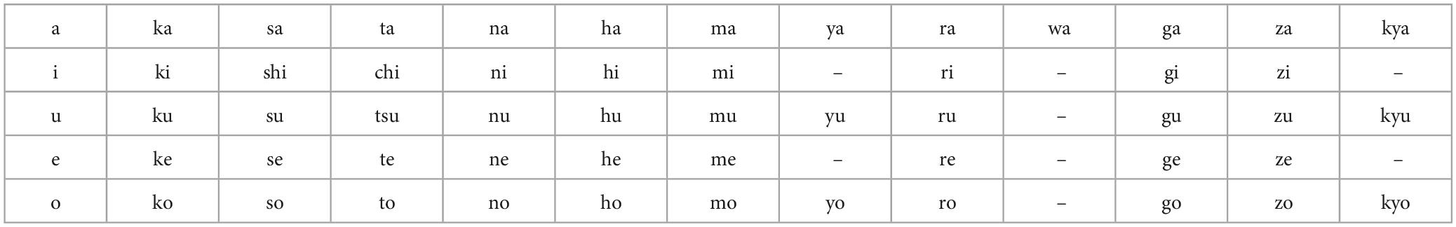
Table 1. Data set of 57 Japanese short syllables.
Figure 3 shows the EEG data timing protocol. Each subject imagines 57 short syllables 5 times.
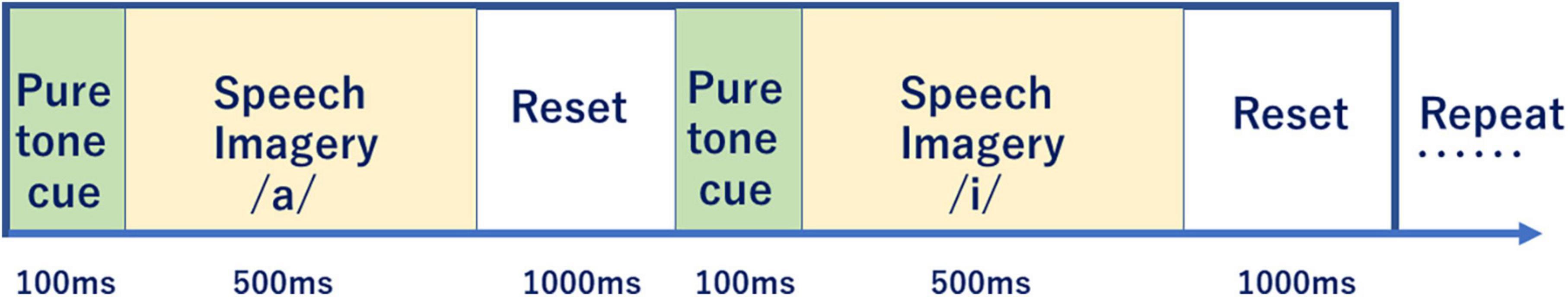
Figure 3. Electroencephalogram data protocol timing.
Electroencephalogram data was preprocessed as follows. First, we removed DC bias from the raw 21-channel EEG signal sampled at 512 [Hz], where DC bias is the averaged value at 100 [ms] intervals, and is reduced from every sample (x(n) - ). Second, a 128-point Fast Fourier Transform (FFT) of the 48 [ms] Hann-windowed segment is applied every 24 [ms] after zero-padding with 104 points to improve the frequency resolution. Third, noise spectrum in EEG is reduced by using a noise spectral subtraction (SS) algorithm (Boll, 1979). We obtain the mean noise spectrum from the initial time slot before starting of the imagined speech, which we subtract from the EEG spectrum X(k) to yield a de-noised EEG (Figure 4 shows the EEG signal of /a/ measured at TP7 before and after SS). Fourth, we apply a band-pass filter (BPF) with a pass band of 80–180 Hz on X(k), and then convert the spectrum to time waveform by applying inverse FFT (IFFT). We use the EEG spectrum of the high-γ band because the literature states that high-order cognitive functions are found in the over-γ band (Heger et al., 2015).

Figure 4. (A,B) Electroencephalogram before and after spectral subtraction (SS).
Figure 5 shows encoding and decoding process of linguistic information L(k) that comprise the LPA of EEG signals in which two-information sources of LPC is modified into one-information source of random signal and then L(k) is convolved. (A) in Figure 5 shows the encoding process of L(k), where the EEG spectrum X(k) is convolved with an input spectrum of random signal W(k) and the spectrum L(k) of linguistic information. Linear prediction of order p in EEG time series {x(n)} is represented by Eq. (1).
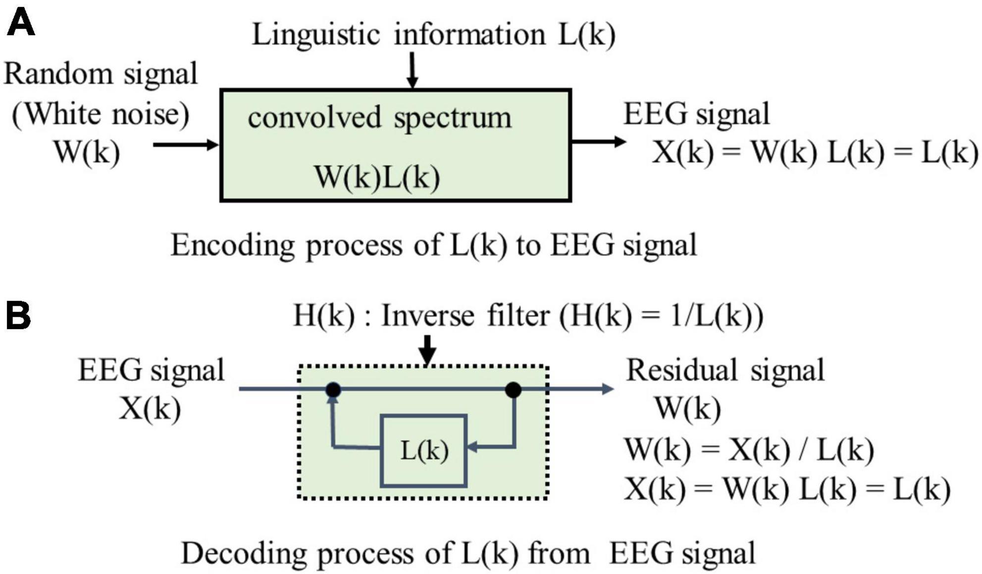
Figure 5. Linear predictive analysis (LPA) for EEG signal.
Eq. (1) shows that the predicted value is represented by linear combination of {xn−p}. Here, the minus sign is for convenience of formula transformation. The squared error e(n)2 is then obtained by the following equation.
A set of {ap} is called linear predictive coefficients that is obtained from autocorrelation coefficients of the EEG time sequence {x(n)} by using Levinson-Durbin’s recursive algorithm (Ramirez, 2008). (B) in Figure 5 shows the decoding process, where the EEG spectrum X(k) is analyzed using an inverse filter H(k) with L(k) in a feedback loop. The EEG spectrum X(k), or the linguistic information spectrum L(k) of each electrode is obtained by Eq. (3):
where ℱ{} is a discrete Fourier transformation (DFT). Eq. (3) is called an all-pole model in LPC. LPC and LPA share an identical framework except that LPA’s sole information source is random noise. We analyze imagined-speech EEGs using LPA by positing an encoding process where linguistic information is convoluted and a decoding process where linguistic information is extracted using an inverse filter. The LPA spectrum L(k) is calculated by Eq. (4) after 0-padding {ap} to arrange the frequency resolution of EEG spectrum.
Figure 6 compares an example of an LPA spectrum versus DFT spectrum. Figure 6 shows three types of LPA spectra that have different lag windows in autocorrelation domain. In this section, we do not use the lag-window, because the LPA spectrum with sharp peak is adequate for converting LPA spectrum to line-spectrum. The LPA spectrum patterns are lastly converted to LPA line-spectrum patterns by using local maximum values and inflection point that are derived from first derivative Δ(k) and second derivative ΔΔ(k); see LPA line-spectra in Figure 6.
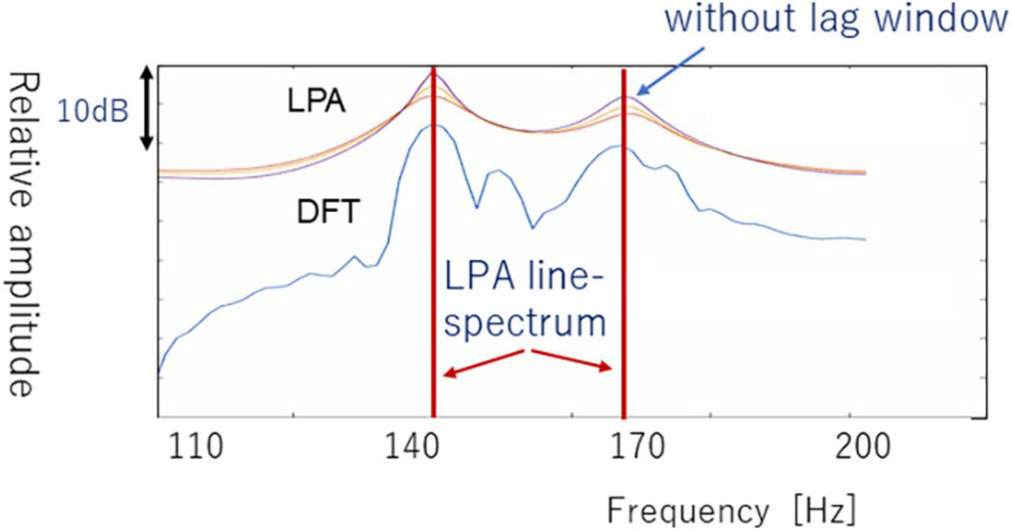
Figure 6. Linear predictive analysis spectrum of a vowel [a] in comparison with DFT spectrum.
In the case of spoken speech (that is, phones or phrases said aloud) observers can synchronize the audio and EEG signals to label speech. In the case of imagined speech however, because there is no reference time signal corresponding to the exact moment the speech was imagined (that is, spoken silently in the human subject’s mind), we need to discover how and where phones or phrases are represented in the multi-channel EEG signal. After analyzing many EEG line-spectra of phones, words, and sentences, we learned that when we integrate (or pool) multi-channel data, chunks of discrete open syllables (that is, consonant-vowel combinations, or CV) having durations of 7–9 frames (56–72 [ms]) become apparent.
Figure 7 shows an EEG line-spectrum sequence that was integrated from 21 electrodes by pooling line spectra. The human subject imagined the Japanese sentence /koNnichiwa/ (”good afternoon”). Because vowels remain stable across multiple frames, CV line spectra resemble V line spectra after pooling. Also noteworthy is the fact that numerous pseudo- (or false or quasi-) short syllables appear in imagined sentences. These pseudo-short syllables seem to arise from sentence-initial /koN/ (N: the Japanese moraic nasal); /ko/ (appearing in frames 282, 320, 332,340, 360), and /N/ (appearing in frames 293, 355). When CV are imagined, many pseudo-short syllables appear alongside true (or real or genuine) speech imagery within the interval of imagined signal. In the next section, we show how we search for vowels from line-spectra data of 21-electrodes with 9 frames.
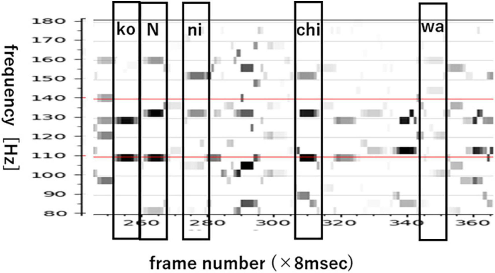
Figure 7. Monosyllable labels of phrase /koNnichiwa/ (good afternoon).
Figure 8 shows the iterative search process for vowel spectra {X(k)} using principle component analysis (PCA) that visualizes linguistic information through eigen-vectors φ(m) and subspace method (SM) that searches the appropriate spectra of vowel for recomposing {X(k)} and redesigning the eigen-vector set. Eq. (5) shows the similarity between a vector X and eigen-vector φ(m) in SM.
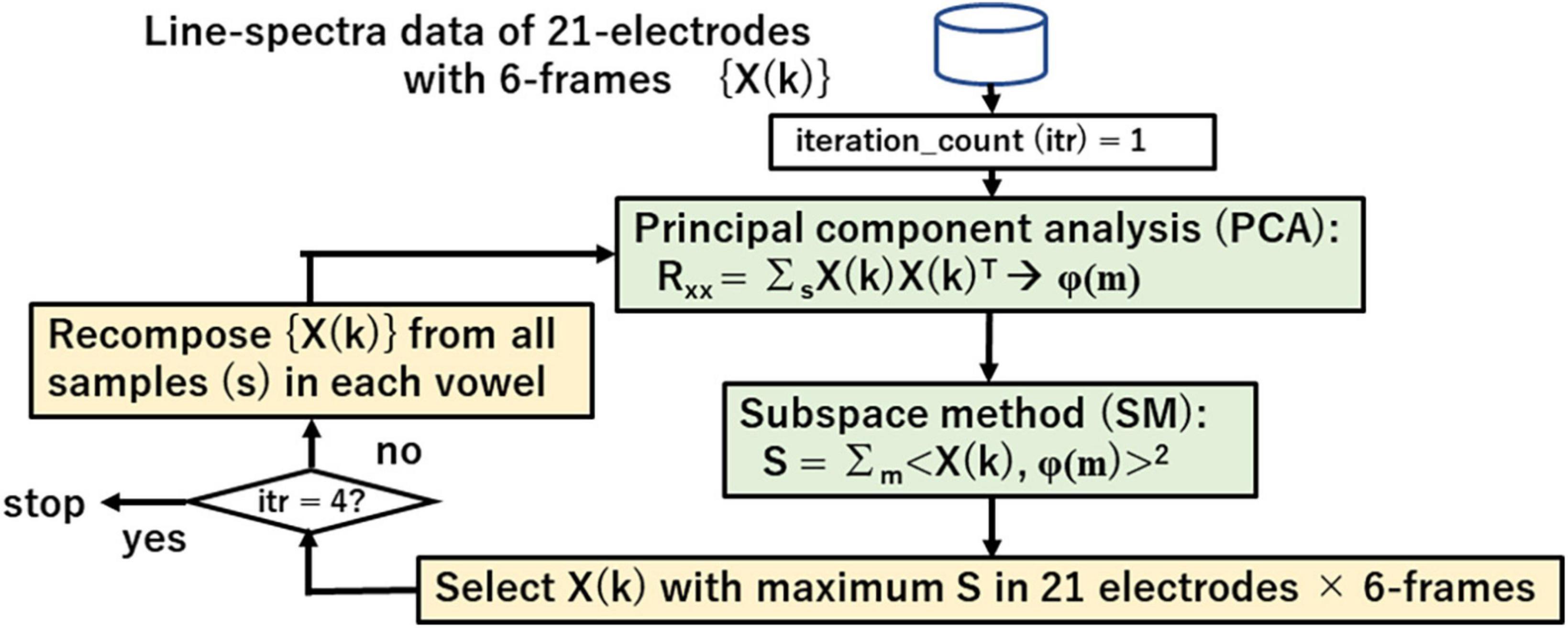
Figure 8. Iterative search for vowel spectra by using principal component analysis (PCA) and subspace method (SM).
Search range is fixed to the last 6 of 9 frames. The iterative search proceeds as follows:
1. Design initial eigen-vectors φ(m) of each vowel from all 21 electrodes and 6 frames.
2. Calculate similarity S between φ(m) and spectra of 21 electrodes and 6 frames.
3. Select spectrum X(k) with maximum S.
4. Recompose {X(k)} from all samples and redesign an eigen-vector set by PCA in each vowel.
5. Repeat steps 2, 3, 4 for 4 iterations.
6. Repeat all steps for all vowels.
Lastly these steps give an eigen space ψ(v, m); v = i, e, a, o, u; m = 1, 2,…, M that represents vowel v.
The resultant eigen space ψ(v, m) likely contains the linguistic representation of vowels. The referencing vector of vowel v is given as Eq. (6).
G(v) is the accumulated spectrum with the weight λ(m)/λ(1). The magnitude of eigen-value λ(m) represents the degree of contribution to G(v).
Figure 9 shows G(v) for 5 vowels /i/ /e/ /a/ /o/ /u/. The 2 spectral peaks (P1, P2) in the upper frequency range remind us of the 2 formant frequencies (F1, F2) in audio spectra of spoken vowels.

Figure 9. Reference vectors of five vowels.
Figure 10 is a scatter plot of P1-P2 values for each of the 5 vowels, with data points from human subjects (4 male, 1 female) and their mean values (Δf = 3.9Hz). Of note is the fact that the 5 vowels in the P1-P2 scatter plot roughly form a line, while cardinal vowels in a F1-F2 plot for spoken speech form a quadrilateral. Also of note is that male and female data points overlap in the P1-P2 scatterplot, while they differ in the spoken vowel F1-F2 plot (Kasuya, 1968).
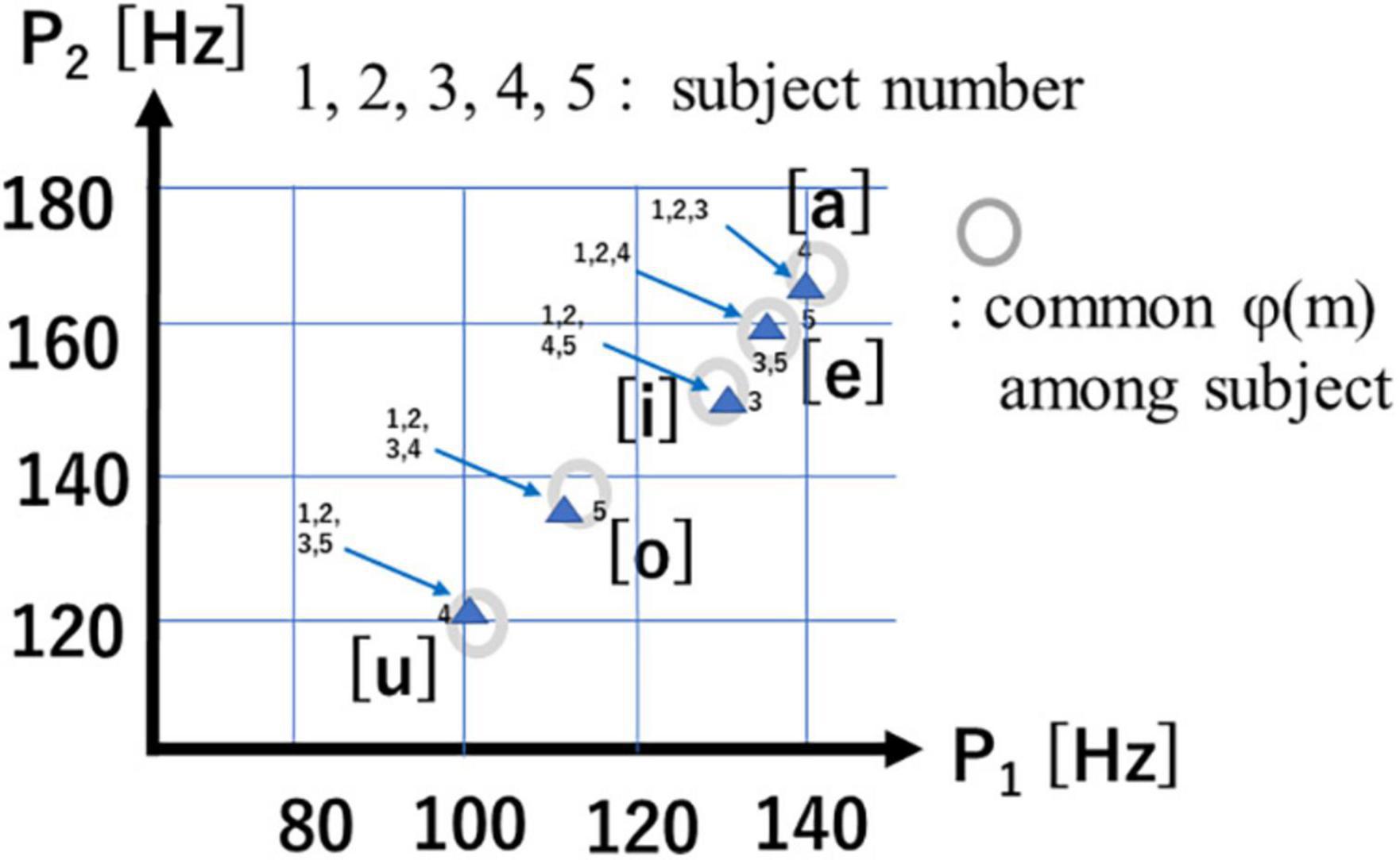
Figure 10. P1-P2 chart of five vowels.
Figure 11 shows a block structure diagram of a subject-independent vowel recognition system prototype that was built to evaluate subject-independent recognition of imagined speech vowels. The vowel classifier compares recognition results of SM and CNN. The CNN is composed of 2-dimensional CNN layers, subsampling layers (2-dimensional pooling), and fully connected layers (multi-layer perceptron or MLP).
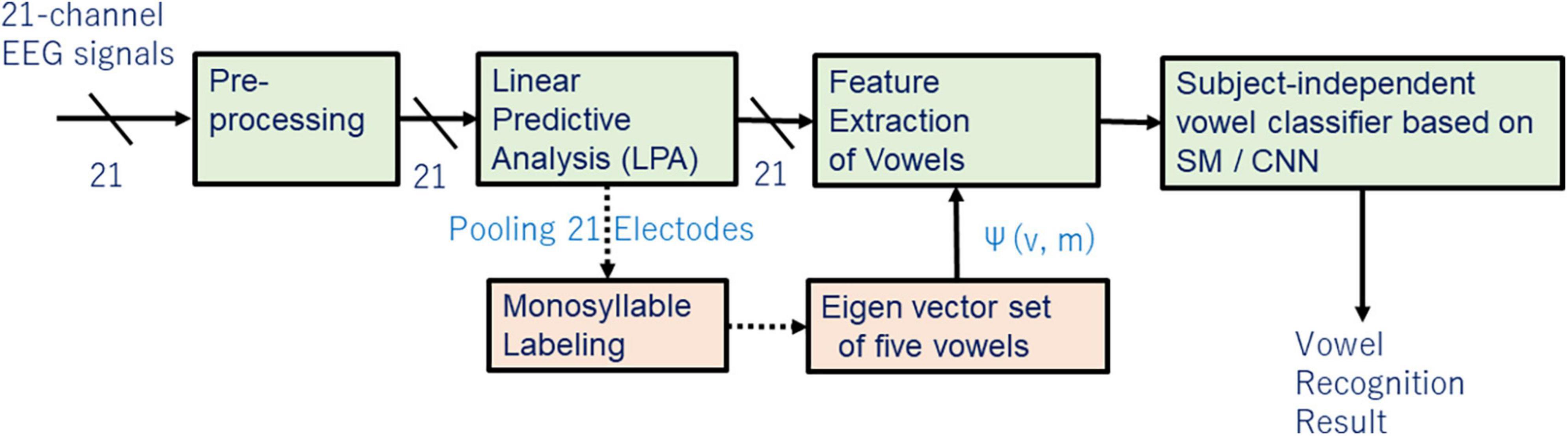
Figure 11. Block structure diagram of subject-independent vowel recognition system prototype.
Figure 12 shows CNN parameters. Recognition accuracies of SM and CNN were measured by using an imagined speech corpora of 5 human subjects. Each human subject imagined the speech of /i/ /e/ /a/ /o/ /u/ 50, 50, 65, 60, 60 times respectively, for a total of 285 samples per human subject, yielding 285 × 5 = 1425 samples in the entire data set. These vowels were taken from the 57 CV in Table 1.
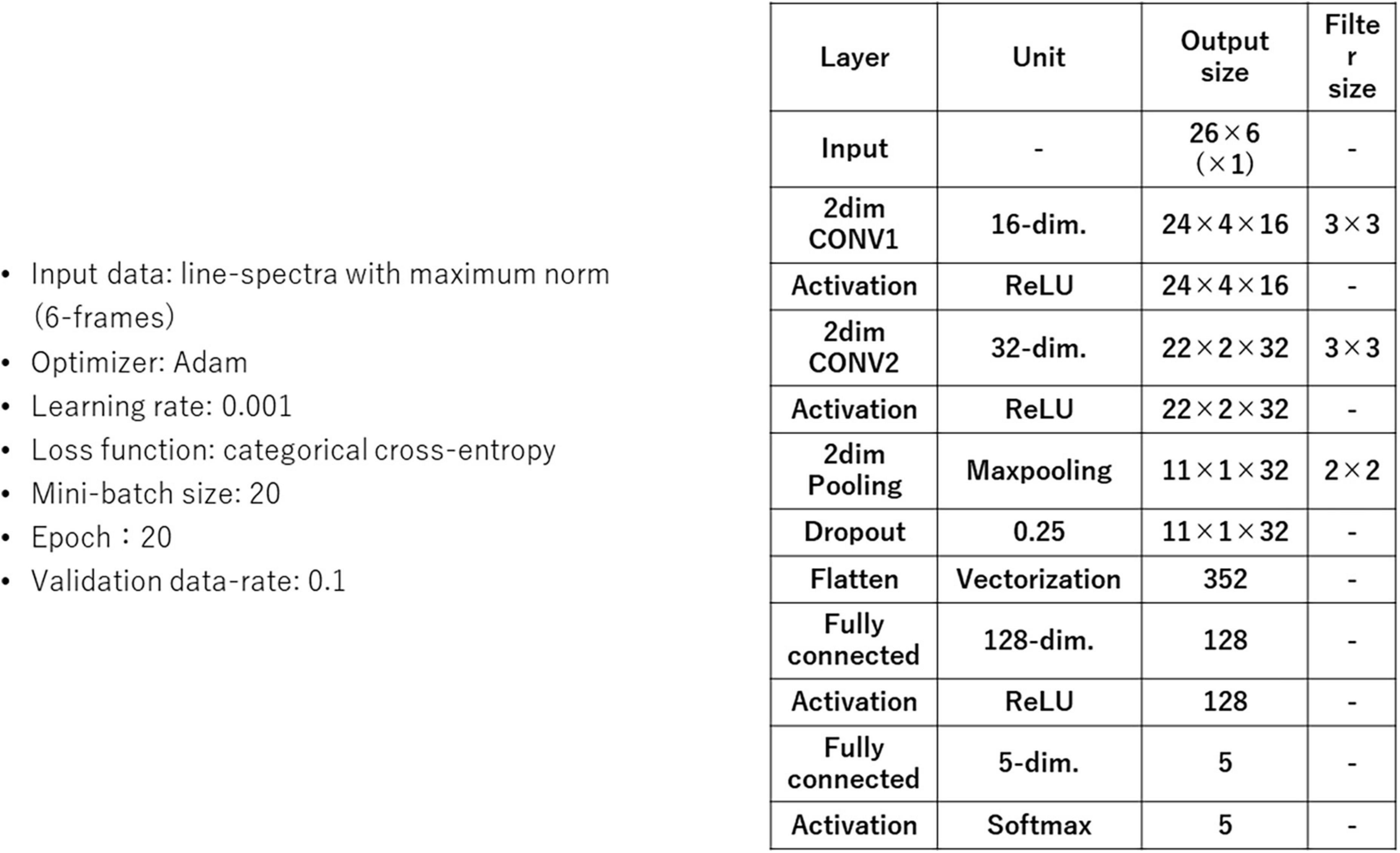
Figure 12. Convolutional neural network (CNN) parameters.
We trained and tested using a so-called jack-knife technique, where 4 of the 5 human subjects were used as training data, the remaining 1 human subject was used as the test data, and we repeated training and testing by alternating training and test data for all human subjects, resulting in cross-validation across 5 human subjects (that is, 1425 × 4 = 5700 samples for training, and 1425 × 1 = 1425 samples for testing). Table 2 shows results of 2 recognition experiments for imagined vowels.
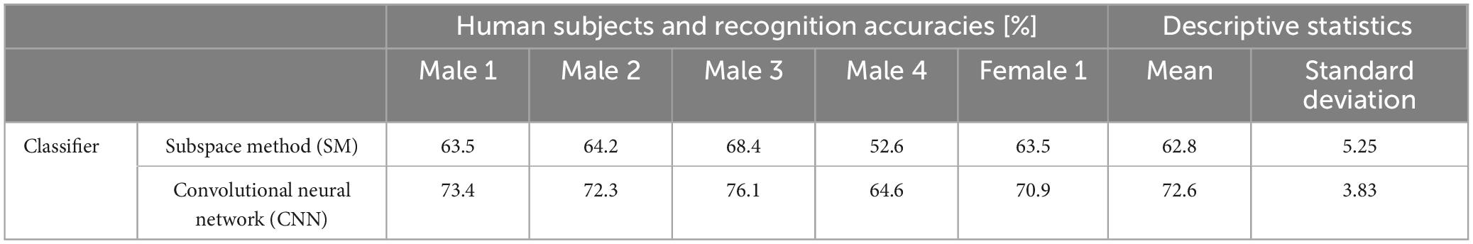
Table 2. Recognition accuracies of imagined speech vowels.
Until now, measurements of linguistic activity in the brain have been limited to where information, that is, location measured by using PET or fMRI for instance. By contrast, what information, that is, how linguistic information is being realized, has been largely neglected. This paper described the following:
1. Hand-labeled short syllable data is extracted from the LPA line-spectra of scalp EEG signals after a pooling process.
2. Iterative search processes of PCA and SM derive eigen-vector sets for 5 vowels.
3. The reference vector G(v) of each vowel calculated from an eigen-vector set φ(m) of line spectra probably contains vowel-specific information.
4. Two prominent spectral peaks (P1, P2) are observed in the upper frequency range, and the 5 vowels are aligned on the P1-P2 chart.
5. The P1-P2 chart suggests that there are no differences in speech imagery between male and females, which would be consistent with the lack of sex differences in EEG signals.
6. A CNN-based classifier obtained a mean recognition accuracy of 72.6% for imagined speech vowels collected from 4 male and 1 female human subjects (however, Male 4 had lower accuracy).
Lopez-Bernal et al. (2022) recently reviewed studies of decoding the EEG of imagined 5 vowels. Recognition results are divided curiously into 2 groups: (1) poor performance below 40% (Cooney et al., 2020), and (2) better performance exceeding 70% (Matsumoto and Hori, 2014). Techniques that do not use labeled EEG data have no choice but to use the whole time duration (typically 1 to 2 [s]) of imagined speech to train the recognizer. Because numerous pseudo-short syllables appear alongside imagined speech, the better-performing recognizers, particularly for vowel recognition, benefit from an abundance of the same short syllables containing the vowel to be recognized. By contrast, when sentences are imagined, only the short syllable at the beginning of the sentence is abundant, and because it differs from other short syllables within the sentence, recognition accuracy may deteriorate.
Our next steps for discovering the linguistic representation in EEGs are (a) extract consonant information, (b) improve recognition accuracy of vowels and consonants, partly by increasing the imagined speech corpora, and (c) build decoding modules for isolated words and/or connected phrases for the purpose of BCI applications.
Incidentally, we are fascinated that EEG line spectra and atomic line spectra closely resemble each other.
The original contributions presented in this study are included in the article/supplementary material, further inquiries can be directed to the corresponding author.
The studies involving human participants were reviewed and approved by YI, Aichi Prefectural University. The patients/participants provided their written informed consent to participate in this study.
TN, GK, and JH conceived the presented idea. YI, JH, and TN collected the EEG data. TN and YI carried out the data processing and analysis. RT and TN developed a labeling tool and labeled monosyllables on EEG data. KK and SS programed and evaluated the classification of vowel using DNN. TN wrote the manuscript with support from GK. All authors contributed to the article and approved the submitted version.
This work was supported by JSPS KAKENHI (Grant Number: JP20K11910).
We thank the reviewers for their feedback. We believe that their suggestions have greatly enhanced the quality of our manuscript.
The authors declare that the research was conducted in the absence of any commercial or financial relationships that could be construed as a potential conflict of interest.
All claims expressed in this article are solely those of the authors and do not necessarily represent those of their affiliated organizations, or those of the publisher, the editors and the reviewers. Any product that may be evaluated in this article, or claim that may be made by its manufacturer, is not guaranteed or endorsed by the publisher.
Anumanchipalli, G. K., Chartier, J., and Chang, E. F. (2019). Speech synthesis from neural decoding of spoken sentences. Nature 568, 493–498. doi: 10.1038/s41586-019-1119-1
Boll, S. F. (1979). Suppression of acoustic noise in speech using spectral subtraction. IEEE Trans. ASSP 27, 113–120. doi: 10.1109/TASSP.1979.1163209
Bouchard, K. E., Mesgarani, N., Johnson, K., and Chang, E. F. (2013). Functional organization of human sensorimotor cortex for speech articulation. Nature 495, 327–332. doi: 10.1038/nature11911
Cooney, C., Korik, A., Folli, R., and Coyle, D. (2020). Evaluation of hyperparameter optimization in machine and deep learning methods for decoding imagined speech EEG. Sensors (Basel) 20:4629. doi: 10.3390/s20164629
Flinker, A., Korzeniewska, A., Shestyuk, A. Y., Franaszczuk, P. J., Dronkers, N. F., Knight, R. T., et al. (2015). Redefining the role of Broca’s area in speech. Proc. Natl. Acad. Sci. U.S.A. 112, 2871–2875. doi: 10.1073/pnas.1414491112
Heger, D., Herff, C., Pesters, A., Telaar, D., Brunner, P., Schalk, G., et al. (2015). “Continuous speech recognition from ECoG,” in Proceedings of the interspeech conference, Dresden, 1131–1135.
Herff, C., and Schultz, T. (2016). Automatic speech recognition from neural signals: a focused review. Front. Neurosci. 10:429. doi: 10.3389/fnins.2016.00429
Indefrey, P., and Levelt, W. J. (2004). The spatial and temporal signatures of word production components. Cognition 92, 101–144. doi: 10.1016/j.cognition.2002.06.001
Itakura, F., and Saito, S. (1968). “Analysis synthesis telephony based on the maximum likelihood method,” in Proceedings of the 6th international congress on acoustics, Tokyo, 17–20.
Kasuya, H. (1968). Changes in pitch and first three formant frequencies of five Japanese vowels with age and sex of speakers. J. Acoustic Soc. Japan 24, 355–364.
Knight, R. T., and Heinze, H.-J. (2008). The human brain: The final journey. Front. Neurosci. 2–1, 15–16. doi: 10.3389/neuro.01.020.2008
Levelt, W. (1993). Speaking: From intention to articulation (ACL-MIT Series in Natural Language Processing). Cambridge, MA: MIT Press.
Lopez-Bernal, D., Balderas, D., Ponce, P., and Molina, A. (2022). A state-of-the-art review of EEG-based imagined speech decoding. Front. Hum. Neurosci. 16:867281. doi: 10.3389/fnhum.2022.867281
Martin, S., Iturrate, I., Millán, J. D. R., Knight, R. T., and Pasley, B. N. (2018). Decoding inner speech using electrocorticography: Progress and challenges toward a speech prosthesis. Front. Neurosci. 12:422. doi: 10.3389/fnins.2018.00422
Matsumoto, M., and Hori, J. (2014). Classification of silent speech using support vector machine and relevance vector machine. Appl. Soft Comput. 20, 95–102.
Miller, K. J., Hermes, D., and Staff, N. P. (2020). The current state of electrocorticography-based brain-computer interfaces. Neurosurg. Focus. 49:E2. doi: 10.3171/2020.4.FOCUS20185
Min, B., Kim, J., Park, H. J., and Lee, B. (2016). Vowel Imagery decoding toward silent speech BCI using extreme learning machine with electroencephalogram. Biomed. Res. Int. 2016:2618265. doi: 10.1155/2016/2618265
Pasley, B. N., David, S. V., Mesgarani, N., Flinker, A., Shamma, S. A., Crone, N. E., et al. (2012). Reconstructing speech from human auditory cortex. PLoS Biol. 10:e1001251. doi: 10.1371/journal.pbio.1001251
Ramirez, M. A. (2008). A Levinson algorithm based on isometric transformation of Durbin’s. IEEE Signal Process. Lett. 15, 99–102.
Rojas, D. A., and Ramos, O. L. (2016). Recognition of Spanish vowels through imagined speech by using spectral analysis and SVM. J. Info. Hiding Multimedia Signal Proces. Ubiquitous Int. 7:4.
Wang, R., Perreau-Guimaraes, M., Carvalhaes, C., and Suppes, P. (2012). Using phase to recognize English phonemes and their distinctive features in the brain. Proc. Natl. Acad. Sci. U.S.A. 109, 20685–20690. doi: 10.1073/pnas.1217500109
Yoshimura, N., Nishimoto, A., Belkacem, A. N., Shin, D., Kambara, H., Hanakawa, T., et al. (2016). Decoding of covert vowel articulation using electroencephalography cortical currents. Front. Neurosci. 10:175. doi: 10.3389/fnins.2016.00175
Yu, Y. H., and Shafer, V. L. (2021). Neural representation of the English vowel feature [high]: evidence from /ε/ vs. /I/. Front. Hum. Neurosci. 15:629517. doi: 10.3389/fnhum.2021.629517
Keywords: EEG, speech imagery, linguistic representation, vowels, labeling syllables
Citation: Nitta T, Horikawa J, Iribe Y, Taguchi R, Katsurada K, Shinohara S and Kawai G (2023) Linguistic representation of vowels in speech imagery EEG. Front. Hum. Neurosci. 17:1163578. doi: 10.3389/fnhum.2023.1163578
Received: 10 February 2023; Accepted: 27 April 2023;
Published: 18 May 2023.
Edited by:
Keun-Tae Kim, Korea Institute of Science and Technology (KIST), Republic of KoreaReviewed by:
Jerrin Thomas Panachakel, College of Engineering Trivandrum, IndiaCopyright © 2023 Nitta, Horikawa, Iribe, Taguchi, Katsurada, Shinohara and Kawai. This is an open-access article distributed under the terms of the Creative Commons Attribution License (CC BY). The use, distribution or reproduction in other forums is permitted, provided the original author(s) and the copyright owner(s) are credited and that the original publication in this journal is cited, in accordance with accepted academic practice. No use, distribution or reproduction is permitted which does not comply with these terms.
*Correspondence: Tsuneo Nitta, bml0dGF0c3VuZW80QGdtYWlsLmNvbQ==
Disclaimer: All claims expressed in this article are solely those of the authors and do not necessarily represent those of their affiliated organizations, or those of the publisher, the editors and the reviewers. Any product that may be evaluated in this article or claim that may be made by its manufacturer is not guaranteed or endorsed by the publisher.
Research integrity at Frontiers
Learn more about the work of our research integrity team to safeguard the quality of each article we publish.