On the Coevolution Between Social Network Structure and Diffusion of the Coronavirus (COVID-19) in Spatial Compartmental Epidemic Models

In this article, the author studies epidemic diffusion in a spatial compartmental model, where individuals are initially connected in a social or geographical network. As the virus spreads in the network, the structure of interactions between people may endogenously change over time, due to quarantining measures and/or spatial-distancing (SD) policies. The author explores via simulations the dynamic properties of the coevolutionary process linking disease diffusion and network properties. Results suggest that, in order to predict how epidemic phenomena evolve in networked populations, it is not enough to focus on the properties of initial interaction structures. Indeed, the coevolution of network structures and compartment shares strongly shape the process of epidemic diffusion, especially in terms of its speed. Furthermore, the author shows that the timing and features of SD policies may dramatically influence their effectiveness.

1. Introduction

In the last two years, the still ongoing diffusion of the Coronavirus disease 2019 (COVID-19) pandemic has spurred a large body of scientific contributions, attempting to explore how compartmental models (Keeling and Rohani, 2008; Pastor-Satorras et al., 2015; Kiss et al., 2017) can reproduce and predict the spread of the epidemics in different countries and regions (Adam, 2020; Kousha and Thelwall, 2020).

Most of this work has been focusing on models in which the mixing process between people in different states or compartments does not depend on the social or geographical space where they are embedded in. However, some previous literature has shown that the (complex) structure of networks describing the way agents can meet and possibly get infected may affect the dynamics of the epidemic diffusion and its long-run properties (Keeling and Eames, 2005; Jin et al., 2014). Furthermore, as the virus spreads in the network, the structure of interactions between people may change over time, due to quarantining measures and/or SD policies, which may possibly introduce a coevolutionary effect dynamically linking disease diffusion and network properties (Achterberg et al., 2020; Horstmeyer et al., 2020; Corcoran and Clark, 2021).

Motivated by these observations, the paper introduces a generalized spatial susceptible, exposed, infected, recovered, dead (SEIRD) model that, besides the standard four compartments (susceptible, exposed, infected, recovered, dead), also considers an additional “quarantined” state, i.e., a susceptible, exposed, infected, quarantined, recovered, dead (SEIQRD) model (Peng et al., 2020).¹ The author explores how the properties of the spread of the epidemics depend on: (i) the structure of the social/geographic network initially connecting the agents in the population, which matches infective and susceptible agents and (ii) the evolution of the share of quarantined and recovered agents (as well as social distancing policies), which dynamically destroy or re-establish social links.

More specifically, the author plays with a finite population of agents (i.e., nodes) initially placed on four different families of interaction structures: (a) regular 2-dimensional lattices with Moore neighborhoods; (b) small-world lattice (Watts and Strogatz, 1998); (c) Erdös-Renyi random graphs (Erdos and Renyi, 1960); and (d) scale-free (preferential-attachment) networks (Barabasi and Albert, 1999). The author then investigates via Monte-Carlo simulations of how the epidemic diffusion is affected by network structures, as their initial average degree increases (which in turn makes their topological properties change) and as the coupled dynamics of quarantined and recovered people deletes and restores social interaction links. Finally, the author examines how alternative SD policies, which are taking again center stage in the political and social debate as to the second wave of COVID-19 rolls across Europe and elsewhere, interact with the coevolutionary process of disease diffusion and network updating.

2. Methods

2.1. A Simple Model Without SD Policies

The author begins by describing a simple model where no SD policies are enforced. Consider a population P of N agents living in a city, which is initially isolated from other cities. Time is discrete and, for the only sake of convenience, the author uses the terms “time periods” or “days” as synonyms. Agents physically interact according to a simple, undirected, binary graph without self-loops, which at time t = 0 is defined as G₀ = (P, L₀), where P = {1, …, N} and L₀ is the initial edge list, defined as the set of pairs (i, j) such that i ≠ j, i ∈ P, j ∈ P, and (i, j) ∈ L₀ if and only if there exists an edge between i and j at t = 0. The graph G₀—which, as we will see below, is going to evolve through time as the epidemics spreads—can be considered as describing social or geographical links through which people normally meet friends or neighbors.

At time t = 0, all nodes are in the state S (susceptible), but a randomly-chosen share θ of them becomes exposed (i.e., ⌊θN⌋ agents become in state E, due to a random inflow of infective agents from other cities). People in state E enter an incubation period without any symptoms and are not infectious. At any t > 0, the author assumes that each agent i ∈ P meets all its neighbors, i.e., all j ∈ V_it, where V_it = {j ∈ P:(i, j) ∈ L_t} and L_t is the current edge list. In each time period, transitions between compartments (i.e., states) occur through a parallel updating mechanism according to the following rules:

(a) An agent in state E becomes state I (infective) after incubation of ⌊Δ⌋ time periods, where Δ is an i.i.d random variable with probability distribution p(Δ). Following (Lauer et al., 2020), we assume that Δ is log-normally distributed with parameters (μ, δ) (refer to Section 2.3 below for more details).

(b) An agent in state E becomes infected with probability π = 1 − (1 − α)^k if s/he meets k infective agents in its neighborhood, where α is a parameter tuning the likelihood of becoming infected in a single direct meeting and 0 ≤ k ≤ |V_it|.²

(c) An agent in the state I becomes quarantined (in state Q) with a daily quarantine rate (DQR_t). Agents in state Q cannot meet anyone, i.e., they instantaneously cut all their bilateral links with their neighbors.³

(d) An agent in state Q dies (i.e., becomes in state D) with a daily death rate (DDR_t), recovers (in state R) with a daily recovery rate (DRR_t), or stays quarantined otherwise. Recovered agents are assumed to be immunized and re-establish connections that they used to have in G₀ (provided that neighbors are still alive and are not quarantined).

A flow-chart description of model dynamics is provided in the Supplementary Material (SM), as shown in Supplementary Figure 1.

2.2. Initial Network Structures

The initial network G₀ is assumed to belong to one out of the following graph families:

 (i) Regular 2-dimensional boundary-less lattices endowed with the Chebyshev distance (LA henceforth, lattice network). This defines squared Moore neighborhoods of radius r^LA ≥ 1 and degrees $k_i^{LA}={(2r^{LA}+1)}^2-1$ for all i.

(ii) Small-worlds lattice (Watts and Strogatz, 1998) built starting from nodes placed on a ring, with rewiring probability p^SW > 0 and expected average degree ${\bar{k}}^{SW}=2r^{SW}$, where r^SW ≥ 1 is the interaction radius on the initial ring (SW henceforth, small-world network).

(iii) Erdös-Renyi random graphs (Erdos and Renyi, 1960), with link probability p^ER > 0 and expected average degree ${\bar{k}}^{ER}=(N-1)p^{ER}$ (ER henceforth, ErdŁos-Renyi network).

(iv) Scale-free networks with linear preferential-attachment (Barabasi and Albert, 1999) and entrance of m^SF ≥ 1 new nodes, generating an expected average degree $\bar{k}=2m^{SF}+o(1/m^{SF})$ (SF henceforth, scale-free network).

These four graph families have been chosen as they represent the simplest and most widely used network structures employed in the literature. Nevertheless, additional, more complex graph families can be employed to describe the initial social or geographical setup, e.g., graphs displaying self-similarity and multi-fractal patterns (Song et al., 2005).

To summarize network topology, the author focuses, besides average degree, on three statistics that have been found to influence, in general, the spread of epidemics on graphs (Lloyd and Valeika, 2005). These are the standard deviation of node degree distribution (s_k), global clustering coefficient (c), and average path-length (ℓ), computed ignoring infinite path-lengths between nodes of different components. Their expected values (with SE) are reported in Supplementary Table 2. To get a better feel, fixing r^LA ∈ {1, 2, 3, 4} and thus $\bar{k}\in \left\{8,24,48,80\right\}$, s_k, c, and ℓ approximately scale as ${\bar{k}}^{\beta }$, with β > 0 for s_k and c and β < 0 for ℓ in all networks.

2.3. Parameter Setup

All simulations refer to a population of N = 1,024 agents (chosen to build a square lattice with edge L = 32) and a number of days T sufficient to reach a steady state.

The epidemic parameters of the model are calibrated using data at the national level for Italy, made available by “Dipartimento della Protezione Civile,” see https://github.com/pcm-dpc/COVID-19, covering the period from February, 22nd onward. In the simulations, the author assumes for simplicity that DRR_t = DRR, DQR_t = DQR, and DDR_t = DDR and, on the basis of empirical diffusion curves, the author builds three epidemic scenarios: (i) strong-impact scenario: (DQR, DDR, DRR) = (0.20, 0.10, 0.10); (ii) mid-impact scenario: (DQR, DDR, DRR) = (0.15, 0.07, 0.15); and (iii) low-impact scenario: (DQR, DDR, DRR) = (0.10, 0.04, 0.20)—(see Supplementary Section S2 for more details). Since the theoretical infection probability in a single meeting cannot be directly observed, the author plays with values of α that are (0.20, 0.10, 0.05), respectively, in the three scenarios. The percentage θ of exposed agents in day 0 is set to 5% throughout. Using results from Lauer et al. (2020), the parameters of the distribution of incubation days Δ are set to (μ, σ) = (1.621, 0.418).

As to initial network structures, the author experiments with average degrees $\bar{k}\in \left\{8,24,48,80\right\}$. These values result from setting r^LA ∈ {1, 2, 3, 4}. Therefore, it follows that r^LA ∈ {4, 12, 24, 40}, $p^{ER}\in \left\{\bar{k}{(N-1)}^{-1},\bar{k}=8,24,48,80\right\}$, and m^SF ∈ {4, 12, 24, 40}. Refer to Supplementary Table 3, for a summary of parameter setups.

2.4. Monte Carlo Simulations and Statistics

For each choice of model parameters, the author independently runs M = 1,000 simulations. This Monte Carlo sample size is sufficient to get SEs for across-simulation averages small enough to ensure that differences between averages are always statistically significant.

In order to get insights about within-simulation model behavior, the author keeps track of several within-simulation statistics, i.e., computed on each day of the epidemic diffusion. These include population shares in each compartment, death and cure rates, the share of agents who become infected through meetings, and the four network metrics $\bar{k}$, s_k, c, and ℓ—which change across time as the result of the evolution population shares in each compartment. Another statistics of interest is the population-average of the number of neighbors that each I agent has infected daily ($\bar{\rho }$ henceforth; refer to Supplementary Section S3 for details), which can be employed as a rough estimate of the basic reproduction number (R₀) of the epidemics. Finally, the author also explores the spatial correlation coefficients of compartments (SCCC), calculating, for each state {S, E, I, Q, R, D} the fraction of all existing edges in the network whose endpoints end up being in the same state.

To summarize the aggregate behavior of the model (i.e., across runs), the following set of additional statistics are computed: (i) peak-time of infections (PTI), defined as the first day in which the share of infected people reach its overall maximum; (ii) the shares of agents in states {S, I, R, D} at the end of the simulation (EoS) and at PTI; (iii) the sum over all compartments of SCCC at PTI; (iv) the EoS share of agents who become infected through meetings; and (v) the values of network metrics $\bar{k}$, s_k, c, and ℓ at PTI. Furthermore, the author provides an estimate of the first day after which $\bar{\rho }$ goes below one (cf. Supplementary Section S3).

Monte Carlo averages of all the above summarizing statistics will then be compared across initial networks families, initial average degrees, and epidemiological setups.

3. Results

3.1. Anatomy of Within-Simulation Dynamics in a Benchmark Setup

The author begins studying the dynamic behavior of disease spreading across the four network families, focusing on the “Mid Impact” epidemic scenario with $\bar{k}=8$ (refer to Figure 1). Irrespective of the initial network structure, the population converges to a similar share of deaths, but in ER and SF networks, a small percentage of S people still remains. This is more clearly depicted in Supplementary Figure 3, where the time series of population shares for susceptible and dead compartments are plotted comparing their behaviors across graph structures (refer to also the discussion in Section 3.3).

FIGURE 1

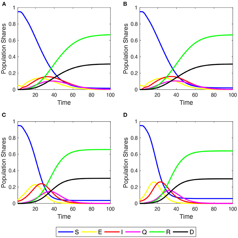
Figure 1. Within-simulation evolution of agent shares in the six compartments over time. Initial $\bar{k}=8$. Mid-impact epidemic scenario. Averages across M = 1,000 Monte Carlo simulations. (A) Regular 2-dimensional lattice with Moore neighborhoods; (B) small-world lattice; (C) Erdös-Renyi random graph; (D) scale-free network.

In these two networks, epidemic diffusion reaches a higher peak of infections than in the case of LA and SW, since more agents become exposed a little earlier. This is because in ER and SF networks the average number of infections per agent grows very quickly during the outbreak of the epidemic process, and then decreases earlier and more sharply than in LA and SW networks (Supplementary Figure 4). The evolution of SCCC shows, indeed, that the shares of edges linking two E or two I agents cross near to PTI and displays a more abrupt inverse-U-shaped pattern over time, illustrating how the virus spreads across neighborhoods (Supplementary Figure 5).

As the epidemic process develops over time, the share of Q agents first grows and then declines. This impacts the network structure, because quarantined agents become isolated, constraining in turn the diffusion of the disease. Furthermore, the more the infection weakens, the more quarantined people recover and re-establish some of their initial connections.

To get a better feel about this coevolutionary process, Figure 2 shows how network metrics, normalized to match the [0, 1] interval, change during a simulation. Both $\bar{k}$ and ℓ decrease toward their minimum value across time in LA and SW, with a pace slowing down as R people spread in the population. The decline of ℓ is due to the growing number of small connected components and isolated nodes created by Q and D agents. In LA and SW networks, however, recovered agents that re-establish their connections are able to slightly boost average degree and reconnect isolated clusters. More marked differences across network structures emerge when looking at s_k and c. In LA, SW and, particularly, in ER graphs, s_k first increases due to the injection of Q agents, then as R and D gradually replace Q patients, it oscillates until getting to a stable level. In SF graphs, instead, s_k follows the same time pattern of $\bar{k}$ and ℓ, as initial heterogeneity is very high and cannot be further increased by the interplay between Q, R, and D shares. Therefore, populations where the epidemics diffuse in LA, SW, and ER networks end up having a higher final heterogeneity of degrees, while the opposite holds for SF graphs. The initial clustering level, instead, is almost completely recovered, but with opposite patterns. LA and SW networks first experience an increase in c (albeit very moderate in magnitude) because the diffusion evolves less quickly. Instead, in ER and SF graphs, some triads are rapidly destroyed by Q people and then R people re-establish them when the epidemics soften. Note also that, unlike what happens in panels (a)–(c), some discontinuities and jumps emerge in the time-series behavior of MC averages of global clustering coefficient. This is not due to an insufficiently large MC sample size, but rather to the well-known sensitivity of clustering coefficients to link dynamics (i.e., link deletion and formation), which occurs throughout our simulations due to quarantines and recoveries (Nakajima and Shudo, 2021). These affect much more the number of triangles present in the network than they do with density, standard deviation of degrees, and average path length.

FIGURE 2

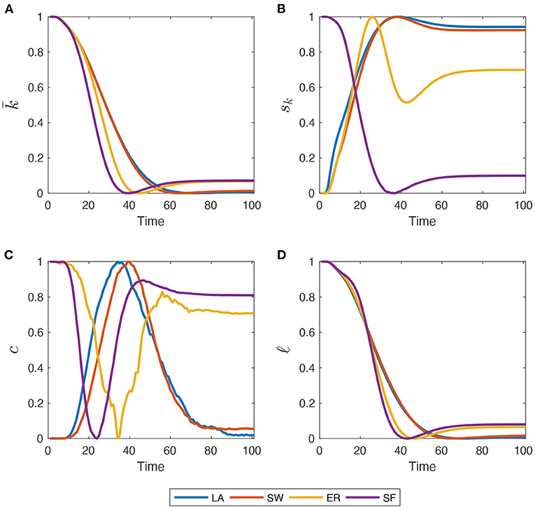
Figure 2. Within-simulation evolution of network metrics, re-scaled to match the [0, 1] interval. (A) Average Degree ($\bar{k}$); (B) standard deviation of node degree distribution (s_k); (C) global clustering coefficient (c); (D) average path-length (ℓ). Initial $\bar{k}=8$ for all four graph families. Mid-impact epidemic scenario. Averages across M = 1,000 Monte Carlo simulations.

In the Supplementary Section S4, the author also shows that, as the share of Q agents first increases and then decreases, and that of R agents keep growing in time, the topological properties of the network change in very heterogeneous ways, depending on the family to which it belongs. This is due to the dynamic removal and re-establishment of links—which affects in non-trivial ways, in particular, the standard deviation of node degrees and global clustering coefficients—and ultimately impacts on the properties of the diffusion process itself.

3.2. The Impact of Initial Average Degree

The author now investigates the behavior of the model when the initial average degree increases in the range of {8, 24, 40, 80}, keeping fixed the epidemic scenario to the “Mid Impact” one. If agents initially have, on average, more neighbors they can meet more infective people. Therefore, the probability to become E increases for the population every single day. However, a larger $\bar{k}$ does not imply that at the end of the simulation (EoS) there will be a larger fraction of deaths and/or recovered, as this is mainly affected by the epidemic parameters. What changes is the speed at which the contagion evolves and some of its dynamic properties.

For example, as shown in Figure 3, both the PTI and the estimate of the first day after which $\bar{\rho }$ goes below one, quickly decrease with $\bar{k}$. Furthermore, as the initial average degree grows, the contagion evolves more quickly in ER and, especially, in SF networks.

FIGURE 3

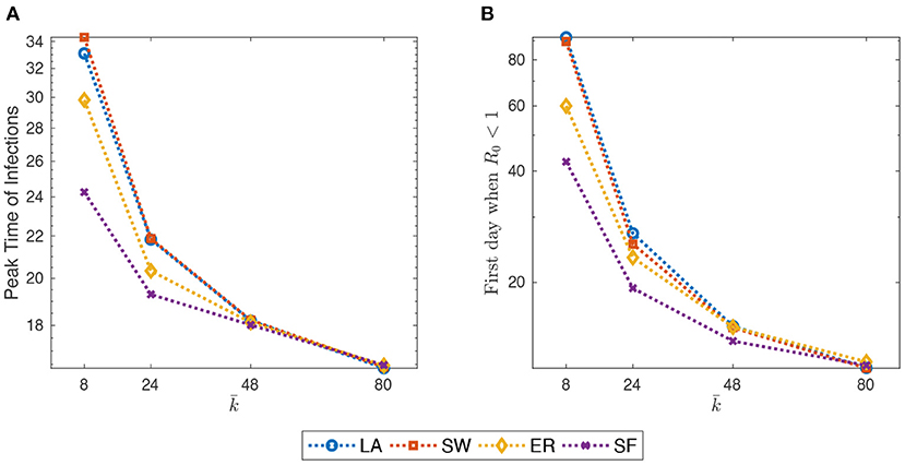
Figure 3. (A) Peak-time of infections (PTI), defined as the first day in which the share of infected people reach its overall maximum, against initial average degree. (B) estimate of the first day after which $\bar{\rho }$ goes below one (cf. Supplementary Section S3). Initial average degree in the range {8, 24, 40, 80}. Mid-impact epidemic scenario. Averages across M = 1,000 Monte Carlo simulations. Y-axis in log scale.

Furthermore, in all networks, the fraction of infected people at PTI immediately jumps up when $\bar{k}$ increases from z 8 to 24, and then keeps growing with $\bar{k}$ but less quickly (cf. Supplementary Figure 6 in the SM). This implies that, since the epidemic scenario is fixed, the share of agents that are quarantined in the first days of the contagion increases more than linearly. Therefore, at PTI, the shares of susceptible, recovered, and dead agents actually decrease with initial average degree.

3.3. Model Behavior in Alternative Epidemic Scenarios

Next, the author explores what happens in the model when alternative epidemic scenarios are assumed (cf. Section 2.3). For the sake of comparison, the author keeps fixed $\bar{k}=8$ throughout. Simulation results show that, as expected, EoS shares of dead (respectively, recovered) agents decrease (respectively, increase) in all network setups as one moves from the bad to the good epidemic scenario (as shown in Figure 4). More interestingly, within the same scenario, the model behaves differently across network setups, and these differences are amplified as the contagion is less strong. Indeed, in ER and SF networks, the epidemics diffuses quicker than in LA and SW graphs—as documented in Supplementary Figures 7A,C. Therefore, LA and SW display more S (and less I) agents at PTI than ER and SW do—as shown in Figure 4C—and a significantly smaller spatial correlation of compartments (in Supplementary Figure 7B). At the end of the simulation (EoS), conversely, many more susceptible agents remain in ER and, especially, in SF networks. This is due to the higher heterogeneity of the degree distribution in such networks: the existence of many small-degree nodes at the beginning of the process prevents them to be infected, especially when the contagion becomes softer and their few neighbors are quickly quarantined. As a consequence, slightly smaller shares of deaths are observed in ER and, in particular, in SF networks at EoS.

FIGURE 4

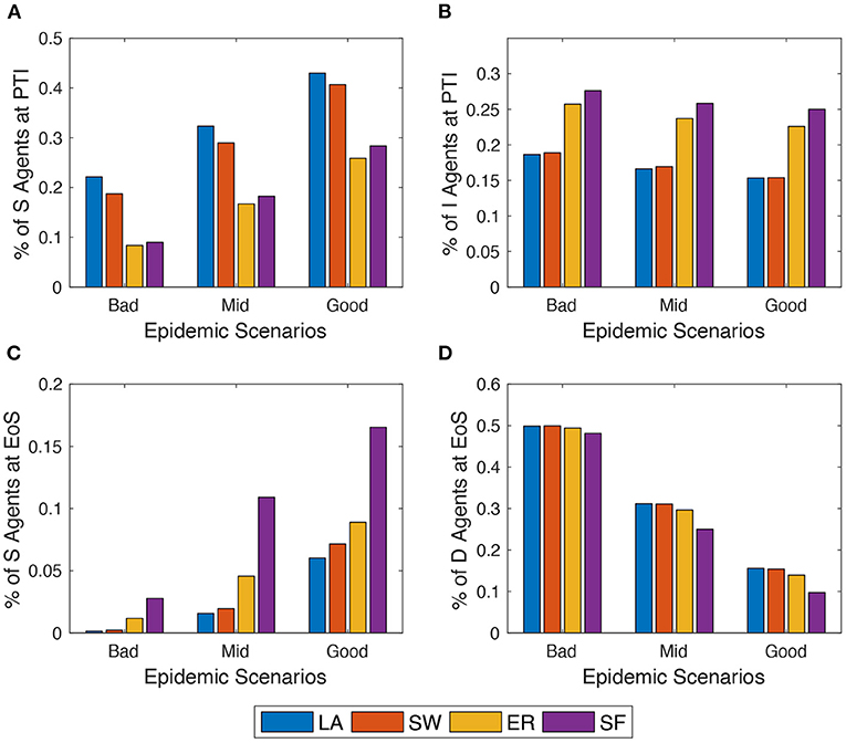
Figure 4. Comparing the behavior of the model across three epidemic scenarios: Bad vs. Mid vs. Good (see Section 2.3). (A) and (C) % of agents in compartment S at peak-time of infections (PTI). (B) % of agents in compartment I at the end of the simulation (EoS). (D) % of agents in compartment D at the EoS. Initial average degree: $\bar{k}=8$. Averages across M = 1,000 Monte Carlo simulations.

3.4. Spatial Distancing

Spatial distancing is implemented in the model in a very stylized way (cf. Achterberg et al., 2020; Horstmeyer et al., 2020; Corcoran and Clark, 2021, for related literature). The author assumes that the city government only tracks the evolution of Q agents and enforces SD when $x_t(Q)>q^{\star }$, where x_t(Q) is the current share of agents in the Q compartment and q^⋆ ∈ (0, 1). The SD policy aims at making more difficult face-to-face meetings between neighbors and can be enforced with increasing strengths. Of course, its ex-post effectiveness also depends on how strictly people follow the rules. Here, the author do not separately model the ex-ante plans of the government and the response of the agents (more on that in Section 4). Therefore, more formally, the author defines θ ∈ (0, 1) as the ex-post effectiveness of SD policy and assume that, under SD, an agent meets each neighbor in any time period t with probability ψ = 1 − θ. This implies that, under SD, an agent in state E now becomes infected with probability:

$\begin{array}{ll}{\pi }^{SD}=1-{(1-\psi \alpha )}^k& (1)\end{array}$

where k is the number of infective agents the agent meets in its neighborhood. The author allows for two versions of SD: (i) permanent, if SD is enforced from the first day when $x_t(Q)>q^{\star }$ onward, i.e., during the period {t, …, T}, where $\underset{\_}{t}={inf}_t\left\{t:x_t(Q)>q^{\star }\right\}$; (ii) temporary, if SD is enforced only whenever $x_t(Q)>q^{\star }$, and it is removed (i.e., θ is switched back to zero) if $x_t(Q)\le q^{\star }-ϵ$. Here, the ϵ-term prevents the SD policy to be too sensitive to oscillations of x_t(Q) around q^*, thus avoiding stop-and-go patterns. In the following simulations, the author considers three SD setups: (a) strong: (q^⋆, θ) = (0.02, 0.7); (b) intermediate: (q^⋆, θ) = (0.04, 0.5); (c) mild: (q^⋆, θ) = (0.06, 0.3), whilst keeping fixed throughout $\bar{k}=8$ in the mid epidemic scenario and ϵ = 0.05.

Figure 5 plots EoS shares of agents under SD (either permanent or temporary) minus the correspondent share without SD. In each SD setup, the author targets the share of people ending up in either S or D compartments and the share of deaths (D). Results show that, as expected, a permanent SD policy is better than a temporary one independently of network structure. However, especially when a strong setup is enforced in the permanent SD policy version, networked populations that benefit the most are those where agents are located on either lattices or small-worlds. Conversely, temporary SD policies are more effective in ER and, in particular, in SF networks, provided that they are implemented more rigorously.

FIGURE 5

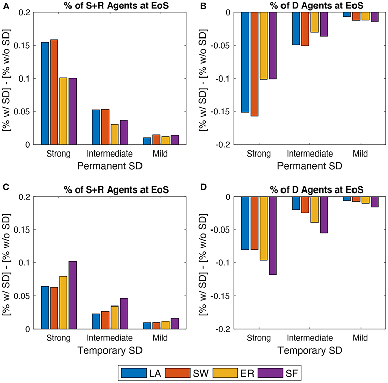
Figure 5. Effects of spatial distancing (SD). Comparing the behavior of the model across three SD setups: Strong vs. Intermediate vs. Bad (see Section 3.4). (A), (B) Permanent SD policy. (C), (D) Temporary SD policy. (A), (C) Share of agents in states S or R at EoS with SD minus the same share without SD. (B), (D) Share of agents in state D at EoS with SD minus same share without SD. Initial average degree: $\bar{k}=8$. Mid epidemic scenario. Averages across M = 1,000 Monte Carlo simulations.

This is due to how network structures evolve during a typical run, as shown in Figure 2. Indeed, when a permanent SD policy is likely to be implemented, LA and SW exhibit larger average degrees and clustering than ER and SF. This prevents the infection to be transmitted more effectively during the peak. Instead, enforcing temporary SD policies allows an even smaller probability that low-degree agents remain susceptible, which is more likely to happen in ER and SF networks, due to their higher degree variability. When such a policy is switched off, ER and SF systems display higher (and more dispersed) average degrees and larger clustering than in the LA and SW cases, but the share of infected people is now smaller. Therefore, one observes less deaths. Disaggregating S and R shares also show that, in the permanent SD case, the improvement in LA and SW is obtained via an almost similar increase of both compartments. On the contrary, when SD is temporary, much of the improvement is due to an increase in EoS susceptible agents only.

4. Discussion

In this article, the author studied a generalized spatial SEIQRD model to explore the impact of alternative social network structures on the diffusion of the COVID-19 disease. The introduction of quarantined agents generates a coevolving process between epidemic spreading and network structure, ultimately shaping steady-state outcomes and the speed of diffusion. In order to make sounder comparisons across different graph structures, the author kept their initial average degree fixed. Therefore, the average degree plays the role of a re-scaling parameter, which is linked to the expected values of the other topological indicators considered (cf. Supplementary Table 2). However, the ensuing dynamics of link deletion and formation due to quarantines and recoveries, structurally changes the graph over time, introducing a two-way causal relationship between the evolving network structure and the diffusion of the disease. This is one of the main contributions of this article, which is nevertheless well-rooted in the literature exploring the impact of alternative network structures on epidemic spreading (also in different application realms, cf. for example Bogdan et al., 2007).

In the simplest framework, without SD policies and a given benchmark choice of initial average degrees and epidemic parameters, the initial network structure does not affect the final shares of susceptible, dead, and recovered people, but it strongly impacts the timing and the speed of diffusion. In ER and, in particular, in SF networks, more agents become exposed earlier and diffusion takes place quicker and more strongly than in the LA and SW cases. This is linked with how network structure coevolves across time with the shares of Q, R, and D agents. Indeed, in ER and SF networks, the average degree initially decreases less sharply than it does in LA and SW. Furthermore, degree variation and clustering are higher. Therefore, the probability of becoming exposed increases, as susceptible agents face larger and more clustered neighborhoods. Increasing initial average degree, while keeping fixed epidemic parameters, thus results in a faster speed of infection, especially in ER and SF networks, both in terms of smaller PTIs and average number of neighbors that each agent has infected daily. When instead different epidemic scenarios are assumed for a fixed initial degree, network structure impacts differently model behavior, and these differences are amplified as the strength of the contagion weakens.

In particular, since the epidemics initially diffuses quicker in ER and SF networks, one typically observes more S (and less I) agents at PTI in LA and SW graphs, and many more remaining S agents at EoS in ER and SF networks (with slightly smaller shares of deaths). This is interesting, as it suggests that societies, where people are initially linked in random or scale-free patterns, can be exposed more to subsequent strains (or variants) of the same virus.

The effect of SD policies depends on the strength of the model with which they are enforced, as well as whether they are temporary or permanent. In particular, whereas permanent SD policies allow for better results than temporary ones irrespective of network structure, permanent (and strong) SD measures are more effective in LA and SW structures, whereas temporary (and strong) SD policies should be preferred if interactions occur through ER or SF graphs. This is again due to the interplay between network structure and compartment shares in the evolution of the epidemics. Indeed, switching on and off SD policies may hit the system when the topological properties of its network structure are very different, depending on the initial graph family describing social interactions (cf. Figure 2), for example, suppose that the government enforces a permanent SD policy. Then, given the activation rule, it is likely that this happens when people in LA/SW networks hold many contacts and are very much clustered. On the contrary, individuals living in ER/SF networks are likely to hold fewer links and to be less clustered. Therefore, a permanent SD policy would flatten the curve of infections more effectively in LA/SW networks than in ER or SF around the peak. This results in a more effective outcome in LA/SW networks as compared to ER/SF graphs both in terms of deaths and recoveries, especially when the spatial distance policy is enforced strongly. If instead, the SD policy is temporary, the probability that agents can spread the virus increases also for low degree agents, which are more likely to be present in ER/SF networks. Furthermore, when the temporary SD policy is switched off, people in ER/SF networks are likely to be more clustered and more connected than those living in LA/SW networks (see Figure 2), but the share of infected people is now smaller. Therefore, one observes less deaths in ER/SF setups. In terms of health policy, this might mean that societies where vulnerable people are more secluded (e.g., they live alone in their homes or in small care houses) might benefit more from a strong and permanent SD policy, as compared to societies where vulnerable people live in environments where they can more easily meet individuals holding many connections (e.g., hospitals).

More generally, results suggest that, in order to predict how epidemic phenomena evolve in networked populations, it is not enough to focus on the properties of initial interaction structures. In fact, if the epidemic diffusion requires quarantining people, and possibly enforcing SD policies, the coevolution of network structures and compartment shares strongly shape the way in which the virus spreads into the population, especially in terms of its speed. On the one hand, the average and standard deviation of the degree distribution, as well as clustering, of initial networks are, together with epidemic parameters, important determinants of the subsequent diffusion patterns. On the other hand, the topology of social interaction structures evolves over time, due to the rise and fall of Q, R, and D agents, in different and nontrivial ways across alternative network families, and this, in turn, impacts diffusion patterns. As a result, the timing and features of SD policies may dramatically influence their effectiveness.

The foregoing analysis can be improved in several directions. To begin with, alternative parameterizations for the epidemic process, more in line with evidence from the ongoing second wave, could be tested. Furthermore, it would be interesting to assess the extent to which results are robust to increasing population size, additional network structures (e.g., core-periphery graphs), and different values for the share of agents that become initially exposed. In this last respect, one could also play with alternative assumptions as to the mechanism governing the way in which exposures initially occur, e.g., allowing for the emergence of spatially-clustered exposed agents, instead of just supposing that a randomly-chosen share of people gets infected. One can also perform a deeper analysis to better understand how the topology of network structures influences epidemic diffusion, for example, asking whether centrality indicators such as k-coreness measures (Kitsak et al., 2010; Bae and Kim, 2014) can help in investigating the role of super spreaders (Bi et al., 2020).

The model, as simple as it is, can be extended to explore additional issues related to epidemic spreading in networked populations. For example, the presence of a non-zero share of susceptible agents at the end of the diffusion process, especially when the initial graph looks like a random graph or a scale-free network (cf. Supplementary Figure 3), suggests studying what could happen in the system when successive strains or variants of the disease enter the system, after the structure of the network has been altered due to the previous strain. Additionally, the assumption that individuals in the model act rationally in presence of rules enforced by the government might be relaxed. This may already be done in the baseline model with SD, assuming that a fraction of individuals disobeys distancing rules and keeps interacting with neighbors with a probability ψ = 1, unlike law-abiding citizens (ψ < 1). That boils down to smaller ex-post effectiveness of the SD policy, i.e., a situation similar to what has already been analyzed in mild SD scenarios. More interestingly, no matter whether SD policies are enforced, one may assume that a fraction of infected agents may refuse to be quarantined. As a result, some individuals would stay infected but are neither cured nor quarantined. This would require defining yet another compartment following infection, to which one can associate a larger DDR and a smaller DCR as compared to the rates defined for quarantined individuals. Furthermore, the model might be extended to include vaccination. In that case, with or without SD, one may model situations where individuals may decide whether to be vaccinated or not. For instance, a fraction of susceptible (and exposed) agents may become immune after vaccination and be assimilated to recovered individuals, while others may resist vaccination and keep being susceptible. This could allow studying the role played by increasing shares of “anti-vax” people in the diffusion process. A last, possibly interesting, extension of the model concerns the introduction of mobility. Following insights from recent literature blending epidemic models on networks with agent mobility (Feng et al., 2020; Goel et al., 2021; Huang and Chen, 2022), one might consider separating geographical proximity and social ties. In the foregoing model, those two dimensions are intertwined and individuals always interact with a set of neighbors that may change over time due to quarantines but is initially predetermined. Instead, agents might be placed in a social network but at the same time interact with other individuals as they move across geographical locations. This may introduce more realism into the model and allow one to play with alternative scenarios concerning, e.g., the extent and the frequency of geographical mixing.

Data Availability Statement

The raw data supporting the conclusions of this article will be made available by the authors, without undue reservation.

Author Contributions

GF: wrote the code, performed simulations, and wrote this article.

Conflict of Interest

The author declares that the research was conducted in the absence of any commercial or financial relationships that could be construed as a potential conflict of interest.

Publisher's Note

All claims expressed in this article are solely those of the authors and do not necessarily represent those of their affiliated organizations, or those of the publisher, the editors and the reviewers. Any product that may be evaluated in this article, or claim that may be made by its manufacturer, is not guaranteed or endorsed by the publisher.

Supplementary Material

The Supplementary Material for this article can be found online at: https://www.frontiersin.org/articles/10.3389/fhumd.2022.825665/full#supplementary-material

Footnotes

1. ^see Supplementary Table 1 for the list of acronyms used in this article.

2. ^In other words, π is the probability of being infected by at least one infective neighbor in a random sequence of meetings.

3. ^Since I do not distinguish between mild and severe symptoms in the development of the illness, there is not any difference in the model between being quarantined at home or at the hospital.

References

Achterberg M. A., Dubbeldam J. L., Stam C. J., and Van Mieghem P. (2020). Classification of link-breaking and link-creation updating rules in susceptible-infected-susceptible epidemics on adaptive networks. Phys. Rev. E 101, 052302. doi: 10.1103/PhysRevE.101.052302

PubMed Abstract | CrossRef Full Text | Google Scholar

Adam, D. (2020). The simulations driving the world's response to covid-19. Nature 580, 316–318. doi: 10.1038/d41586-020-01003-6

PubMed Abstract | CrossRef Full Text | Google Scholar

Bae, J., and Kim, S. (2014). Identifying and ranking influential spreaders in complex networks by neighborhood coreness. Phys. A Stat. Mech. Appl. 395, 549–559. doi: 10.1016/j.physa.2013.10.047

CrossRef Full Text | Google Scholar

Barabasi, A.-L., and Albert, R. (1999). Emergence of scaling in random networks. Science 286, 509–512.

Google Scholar

Bi, Q., Wu, Y., Mei, S., Ye, C., Zou, X., Zhang, Z., et al. (2020). Epidemiology and transmission of covid-19 in 391 cases and 1286 of their close contacts in Shenzhen, China: a retrospective cohort study. Lancet Infect. Dis. 20, 911–919. doi: 10.1016/S1473-3099(20)30287-5

PubMed Abstract | CrossRef Full Text | Google Scholar

Corcoran C., and Clark J. M. (2021). Adaptive network modeling of social distancing interventions. arXiv:2102.06990.

Google Scholar

Duncan J. Watts, and Steven H. Strogatz. (1998). Collective dynamics of 'small-world' networks. Nature 393, 440–442.

Google Scholar

Erdos, P., and Renyi, A. (1960). On the evolution of random graphs. Publ. Math. Inst. Hungary. Acad. Sci. 5, 17–61.

Google Scholar

Feng, L., Zhao, Q., and Zhou, C. (2020). Epidemic in networked population with recurrent mobility pattern. Chaos Solitons Fractals 139, 110016. doi: 10.1016/j.chaos.2020.110016

PubMed Abstract | CrossRef Full Text | Google Scholar

Goel, R., Bonnetain, L., Sharma, R., and Furno, A. (2021). Mobility-based SIR model for complex networks: with a case study of COVID-19. Soc. Netw. Anal. Min. 11, 105. doi: 10.1007/s13278-021-00814-3

PubMed Abstract | CrossRef Full Text | Google Scholar

Horstmeyer L., Kuehn C., and Thurner S. (2020). Balancing quarantine and self-distancing measures in adaptive epidemic networks. arXiv:2010.10516.

Google Scholar

Huang, J., and Chen, C. (2022). Metapopulation epidemic models with a universal mobility pattern on interconnected networks. Phys. A Stat. Mech. Appl. 591, 126692. doi: 10.1016/j.physa.2021.126692

PubMed Abstract | CrossRef Full Text | Google Scholar

Jin, Z., Sun, G.-Q., and Zhu, H. (2014). Epidemic models for complex networks with demographics. Math. Biosci. Eng. MBE 11, 1295–317. doi: 10.3934/mbe.2014.11.1295

PubMed Abstract | CrossRef Full Text | Google Scholar

Keeling, M. J., and Eames, K. T.D. (2005). Networks and epidemic models. J. R. Soc. Interface 2, 295–307. doi: 10.1098/rsif.2005.0051

PubMed Abstract | CrossRef Full Text | Google Scholar

Keeling, M. J., and Pejman Rohani, P. (2008). Modeling Infectious Diseases in Humans and Animals. Princeton, NJ: Princeton University Press.

Google Scholar

Kiss, I. Z., Miller, J. C., and Simon, P. (2017). Mathematics of Epidemics on Networks: From Exact to Approximate Models. Cham: Springer.

Google Scholar

Kitsak, M., Gallos, L., Havlin, S., Liljeros, F., Muchnik, L., H. Stanley, et al. (2010). Identification of influential spreaders in complex networks. Nat. Phys. 6, 888–893. doi: 10.3389/fphy.2021.766615

PubMed Abstract | CrossRef Full Text | Google Scholar

Kousha, K., and Thelwall, M. (2020). Covid-19 publications: database coverage, citations, readers, tweets, news, facebook walls, reddit posts. arXiv:2004.10400 [cs.DL].

Google Scholar

Lauer, S. A., Grantz, K. H., Bi, Q., Jones, F. K., Zheng, Q., Meredith, H. R., et al. (2020). The incubation period of coronavirus disease 2019 (COVID-19) from publicly reported confirmed cases: estimation and application. Ann. Internal Med. 3, 1–7. doi: 10.7326/M20-0504

PubMed Abstract | CrossRef Full Text

Lloyd, A. L., and Valeika, S. (2005). Network Models in Epidemiology: An Overview, Ch. 8, London: World Scientific, 189–214.

Google Scholar

Nakajima, K., and Shudo, K. (2021). Measurement error of network clustering coefficients under randomly missing nodes. Sci. Rep. 11, 2815. doi: 10.1038/s41598-021-82367-1

PubMed Abstract | CrossRef Full Text | Google Scholar

Pastor-Satorras, R., Castellano, C., Van Mieghem, P., and Vespignani, A. (2015). Epidemic processes in complex networks. Rev. Mod. Phys., 87, 925–979. doi: 10.1103/RevModPhys.87.925

CrossRef Full Text | Google Scholar

P. Bogdan, T. Dumitras, and R. Marculescu. (2007). Stochastic communication: a new paradigm for fault-tolerant networks-on-chip. VLSI Design 2007, 095348. doi: 10.1155/2007/95348

CrossRef Full Text | Google Scholar

Peng, L., Yang, W., Zhang, D., Zhuge, C., and Hong, L. (2020). Epidemic analysis of covid-19 in china by dynamical modeling. medRxiv, 2020.

PubMed Abstract | Google Scholar

Song, C., Havlin, S., and Makse, H. A. (2005). Self-similarity of complex networks. Nature 433, 392–395. doi: 10.1038/nature03248

PubMed Abstract | CrossRef Full Text | Google Scholar