Addressing GPU memory limitations for Graph Neural Networks in High-Energy Physics applications

Introduction: Reconstructing low-level particle tracks in neutrino physics can address some of the most fundamental questions about the universe. However, processing petabytes of raw data using deep learning techniques poses a challenging problem in the field of High Energy Physics (HEP). In the Exa.TrkX Project, an illustrative HEP application, preprocessed simulation data is fed into a state-of-art Graph Neural Network (GNN) model, accelerated by GPUs. However, limited GPU memory often leads to Out-of-Memory (OOM) exceptions during training, due to the large size of models and datasets. This problem is exacerbated when deploying models on High-Performance Computing (HPC) systems designed for large-scale applications.

Methods: We observe a high workload imbalance issue during GNN model training caused by the irregular sizes of input graph samples in HEP datasets, contributing to OOM exceptions. We aim to scale GNNs on HPC systems, by prioritizing workload balance in graph inputs while maintaining model accuracy. Our paper introduces diverse balancing strategies aimed at decreasing the maximum GPU memory footprint and avoiding the OOM exception, across various datasets.

Results: Our experiments showcase memory reduction of up to 32.14% compared to the baseline. We also demonstrate the proposed strategies can avoid OOM in application. Additionally, we create a distributed multi-GPU implementation using these samplers to demonstrate the scalability of these techniques on the HEP dataset.

Discussion: By assessing the performance of these strategies as data loading samplers across multiple datasets, we can gauge their effectiveness in both single-GPU and distributed environments. Our experiments, conducted on datasets of varying sizes and across multiple GPUs, broaden the applicability of our work to various GNN applications that handle input datasets with irregular graph sizes.

1 Introduction

Neutrinos, the most abundant matter particles in the universe, can answer fundamental questions about the nature of matter and the evolution of the universe. Conducting experiments using advanced tracking algorithms to reconstruct the trajectories of thousands of charged particles from a collision event as they fly through a detector can advance neutrino discoveries (Abi and Acciarri, 2020). To harness this low-level particle data, High Energy Physics (HEP) applications are increasingly developing deep learning (DL) models aimed at reconstructing millions of particle trajectories per second from the petabytes of raw data produced by the next generation of detectors at the Energy and Intensity Frontiers (ExaTrkX Collaboration, 2024). In particular, recent success in using Graph Neural Networks (GNNs) in accurately classifying particle types and edges have prompted multiple scientific workflows based on GNNs (Ju et al., 2021). We use one of these scientific workflows as an illustrative example of an HEP application to demonstrate the current limitations of large-scale GNNs (Lee et al., 2023).

In the deployment of GNNs for particle reconstruction on HPC systems, we rely on GPUs for efficient model training. Currently, GPU utilization remains prevalent for accelerating the training, testing, and deployment of DL models. However, an Out-of-Memory (OOM) exception can arise during model training due to constrained GPU memory space relative to the large CPU memory space. The limited aggregate GPU memory size of state-of-art GPUs amplifies the prevalence of OOM issues in Deep Learning (DL) applications. According to Rajbhandari and Ruwase (2021), while the size of largest training dense model has increased by a factor of 1,000 in recent years, GPU memory has only grown 5-fold from 16 GB (NVIDIA Tesla V100) to 80 GB (NVIDIA Tesla A100). Moreover, an empirical study detailed in Gao et al. (2020), cites the exhaustion of GPU memory as the top reason for failed DL jobs. Consequently, GPU memory limitations pose a bottleneck, particularly when the size of datasets surpass the GPU memory capacity.

The problem of OOM is further exacerbated using GPUs to run model training on large-scale datasets. HPC systems are designed to support larger datasets with a parallel filesystem and stronger processing cores. However, these resources cannot be fully utilized with a limited GPU memory capacity (Pumma et al., 2019; Anonymous, 2003). One proposed strategy for OOM exceptions is reducing the batch size (Yang et al., 2023). However, maintaining a larger batch size provides advantages. First, a larger batch size increases the degree of data parallelism we can exploit on HPC systems. Given a smaller batch size, this upper limit is reached much more quickly. Furthermore, using a larger batch size can increase the number of features we can run with our model. Also, too small of a batch size can hurt model accuracy (Peng et al., 2017).

Previous research employs distributed GNNs such as those presented in Jia et al. (2017), Tripathy et al. (2020), Hu et al. (2021), and Zhu et al. (2019) for scaling GNNs leverages large input graphs as input to the model. However, in our HEP application, each sample constitutes an independent collision event, thus forming individual graphs of moderate sizes. To the best of our knowledge, our work stands as the pioneering attempt to apply such methodologies to datasets comprised of individual graph samples with dynamic sizes.

The HEP application input training samples are comprised of event graphs can differ from each other by an order of magnitude creating a large standard deviation between the sizes of graphs. Therefore, using a naïve random sampler to generate the mini-batches from training may result in a large range in memory size and results in a substantially higher maximum GPU memory consumption value compared to the average size of the samples in the mini-batch. OOM exceptions are caused when the GPU memory spikes to a value above the supported GPU capacity. This GPU memory threshold can be exceeded due to a batch comprised of large graph samples, creating an imbalance among mini-batches. Therefore, we introduce the multiple alternative mini-batch balancing strategies to avoid an OOM exception.

Our paper addresses workload imbalances in GNNs with irregular-sized training samples across various settings by proposing multiple workload-balancing algorithms to redistribute data samples.

We make the following key contributions in this paper. We (1) introduce multiple mini-batch balancing strategies and integrate them into a state-of-the-art HEP GNN model to reduce the maximum GPU memory usage and consequently the probability of an OOM exception on a single-GPU while maintaining accuracy on the full dataset, (2) parallelize the GNN and the mini-batch balancing strategies across multiple GPUs without compromising accuracy to demonstrate the scalability of the strategies, and (3) evaluate the tradeoff between memory conservation and preprocessing overhead of the proposed mini-batch balancing strategies on HPC systems.

In this paper, we describe how the balancing scheme is utilized in the Exa.TrkX workflow to address these challenges and coordinate the data management requirements, using datasets provided by the MicroBoone Collaboration (Abratenko and Aldana, 2022b,a) and the computing and storage resources from the supercomputer Perlmutter (National Energy Research Scientific Computing Center (NERSC), 2024) located at the National Energy Research Scientific Computing Center (NERSC).

2 Background and motivation

2.1 High energy physics workflow

Graph Neural Networks (GNNs) to capture high-level patterns on non-Euclidean datasets have recently received considerable attention in High-energy Physics (HEP) projects, providing promising results for particle track reconstruction and other data analyzes (ExaTrkX Collaboration, 2024). The Exa.TrkX Project, an illustrative HEP application aims to create particle tracking algorithms linearly scales with numerous data points. Geometric Deep Learning (GDL) offers a reasonable solution to both needs of scalability on large datasets and optimal performance on non-Euclidean datasets. Therefore, GNNs are utilized in multiple scientific workflows for HEP collider experiment data (Ju et al., 2021).

One such pipeline is for simulated data from the Liquid Argon Time Projection Chambers (LArTPC) neutrino experiments (Hewes and Aurisano, 2021). The main goal of this application is to semantically label recorded energy depositions, or hits, according to the type of particle that generated them. The raw data consists of petabytes of data but is condensed into graphs through a scientific workflow. The infrastructure of the pipeline, as outlined in Lee et al. (2023), preprocesses simulation data to graph samples. These samples are in turn used as input to a state-of-art GNN model for classification. The simulated data is stored in event graphs with each graph containing a variable number of nodes and edges. Therefore, the graph samples in the dataset have irregular graph sizes.

2.2 Input dataset characterization

Figure 1 shows the dataset exhibits a right-skewed distribution, as illustrated by the histogram. Among the samples, the majority cluster within the 100 MB range. However, as shown by Table 1, the largest sample in the dataset ranges upto an order of magnitude larger compared to the average sample size. Furthermore, the presence of a large standard deviation signals numerous outliers within the dataset.

Figure 1

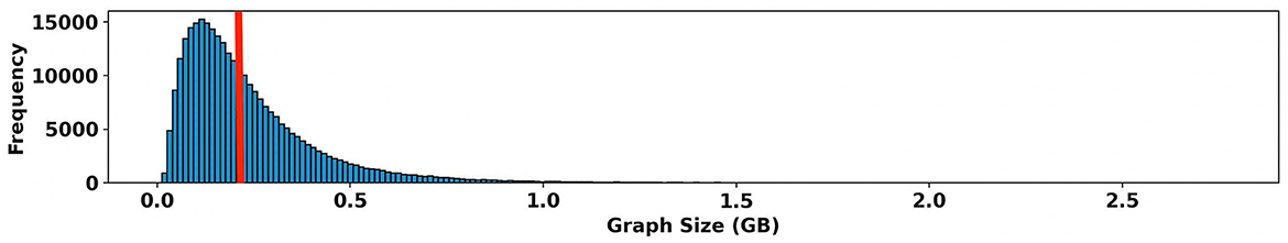
Figure 1. Dataset histogram shows the right-skewedness of the sample sizes. Individual graph samples range from 12 to 2,833 MB. The red line indicates the average graph sample size.

Table 1

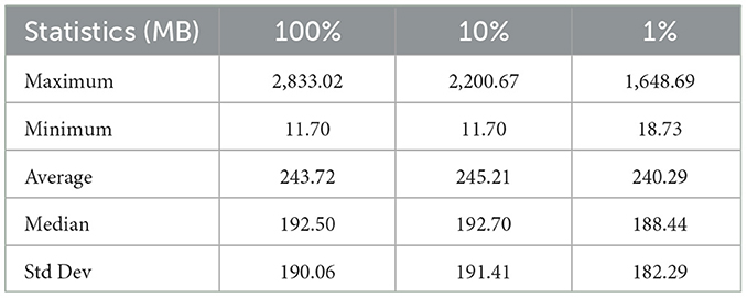
Table 1. Mini-batch statistics given a batch size of 64.

In addition to the original dataset, we meticulously curate two additional smaller datasets derived from the original graph data. These datasets are a subset of the original dataset selected at random to represent a part of the real-world dataset. The reason for creating these datasets is 2-fold. The first is to evaluate the degree of randomness on model performance. As the size of the dataset decreases, the range of samples the data loader can choose from also decreases. We aim to understand how different workload balancing strategies affect factors such as GPU memory footprint and model accuracy. The second is for practical reasons. Running the GNN model until validation loss converges takes ~80 h. A smaller dataset enables faster evaluation of trends in the dataset. Each instance in the dataset represents an event graph depicting a collision event involving sub-atomic particles. Each event graph is assigned a unique event ID corresponding to a continuous time range. We deliberately extract event IDs from this continuous time range to generate datasets with 10 and 1% of the samples present in the original dataset.

To visually represent the distribution of these datasets, we utilize a box and whisker plot (Figure 2). In this visualization, the whisker caps of the box plot denotes the minimum and maximum values within the dataset and the red line in the center of the boxes signifies the median value. The single black circles above the boxes show the outliers. In Figure 2, a large number of outliers is evident in the original dataset. In particular, as the dataset size diminishes to 10 and 1%, the number of outliers in the dataset decreases. However, all datasets maintain sample distribution; the average, median, and standard deviation among the graph samples are nearly the same.

Figure 2

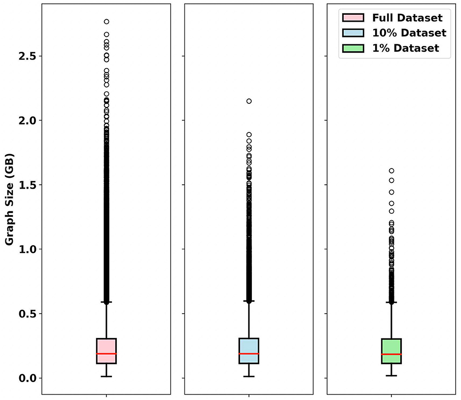
Figure 2. Box plot of different datasets. The dots represent outliers in the dataset. The red line indicates the median and the whisker caps signify the minimum and maximum values of dataset, excluding outliers.

2.3 GPU Out-of-Memory exception

The Out-of-Memory (OOM) exception on GPUs arises when there is insufficient GPU memory during program runtime, particularly in the context of model training. This exception becomes apparent when the GPU memory utilization surges, surpassing the maximum GPU memory capacity. Therefore, lowering the maximum GPU memory footprint emerges as a potential strategy to mitigate the likelihood of encountering OOM exceptions, potentially averting such issues altogether. This strategic adjustment contributes to a more stable and efficient training process in the face of potential OOM challenges.

2.4 Impact of balancing mini-batches on allocated memory

The Pytorch library leverages a CUDA caching memory allocator for efficient management of GPU memory, specifically tailored to optimize memory allocation and deallocation on GPUs (Paszke et al., 2019). Allocated memory represents the current GPU memory occupied by tensors in bytes for a specified device whereas reserved memory monitors the GPU memory actively managed by the caching allocator in bytes for a designated GPU device.

We observe a similarity in the trend between GPU allocated memory (Figure 3) and the batch size in bytes (Figure 4) throughout the training process. To substantiate this correlation, we employ the Pearson Correlation Coefficient (PCC). The PCC, measuring linear correlation on a scale from -1 to 1, signifies stronger correlation with values closer to 1. Our calculated PCC between batch memory consumption and GPU memory allocation at runtime, using the default model setting's batch size (64), yields a robust correlation coefficient of 0.928. Leveraging this insight, we set an objective to balance mini-batch sizes during training to effectively reduce GPU memory consumption.

Figure 3

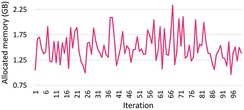
Figure 3. The amount of allocated memory in GB during model training over 100 iterations.

Figure 4

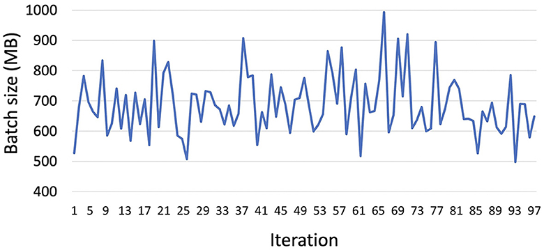
Figure 4. The mini-batch size in MB during model training over 100 iterations.

The irregularities in the size of graph data samples introduce variability, where certain samples may act as outliers, occupying more bytes than others. This discrepancy can lead to an imbalance in mini-batch sizes across different batches. To address this concern, we aim to distribute data samples across all mini-batches, to ensure a balanced size each iteration in terms of GPU memory usage.

2.5 Particle type multiplicity

Within the graph dataset, all graph edges fall into one of four categories: shower-like, muonic, hadronic, and false (Hewes and Aurisano, 2021). The distribution of these particles is detailed in Table 2. The particle types can also be divided into HIP, MIP, EM showers, and Michel electrons. HIP denotes “Heavily Ionizing Particles,” encompassing protons, kaons, nuclei, etc., while MIP represents Minimum Ionizing Particles and consists of particles such as muons, pions, etc. The goal of the semantic label in the GNN is to correctly classify these particle types. Understanding and considering these distinctions in particle types is crucial for a nuanced analysis of the dataset and can inform strategies for improving model accuracy.

Table 2

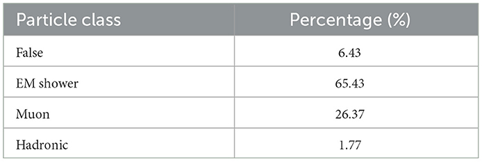
Table 2. The particle type breakdown by percentage.

In our dataset, the multiplicity of samples exhibits a correlation with the subatomic particle type. The number of nodes in the graph is directly linked to the true particle type, influencing the overall graph size in bytes. For instance, particle types like Electromagnetic (EM) showers (Figure 5) typically entail numerous nodes, while a Michel electron features only a few nodes (Figure 6). Therefore, maintaining or improving model accuracy can be facilitated by evenly balancing the batch size in bytes.

Figure 5

Figure 5. EM shower graph.

Figure 6

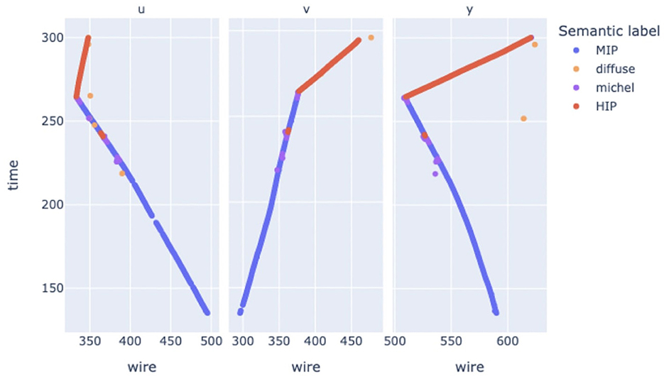
Figure 6. Michel electron graph.

2.6 Degree of randomness

Shuffling input training samples is important for avoiding bias and ultimately providing good generalization for the model. However, the degree of randomness of shuffling can be reduced when training a parallel model with multiple GPU devices. We quantify the degree of randomness to evaluate the impact of the randomness on model accuracy.

Given N training samples, B as the global batch size, at each epoch, there are $\frac{N}{B}$ batches processed. This training epoch is repeated until the validation loss has converged. We assume there are I training epochs in total. In parallel Deep Neural Network training, assuming P as the number of processes, each individual process randomly reads $\frac{B}{P}$ samples at each iteration. Same as the non-parallel training, there are $\frac{N}{B}$ iterations per epoch.

In the context of distributed training across multiple GPUs employing local shuffling, the total of N training samples is uniformly distributed among the available devices. Consequently, each process is allocated $\frac{N}{P}$ samples, where P represents the total number of processes or devices involved (Nguyen et al., 2022). Throughout the training iterations, these assigned samples are locally shuffled, contributing to the diversification of data input for each process. This local shuffling approach ensures that each process works with a distinct subset of training samples, promoting effective exploration of the dataset across the distributed training environment.

3 Design and implementation

3.1 Workload balancing strategies

Each graph sample in the dataset has a varying number of nodes in the graph and consequently a different size. The inherent variability in graph samples within our dataset, manifested through varying node counts and sizes, presents a unique challenge, particularly concerning GPU memory allocation during batching. Aggregating large graph samples with substantial byte sizes into a single batch can significantly inflate the GPU memory footprint, leading to potential memory allocation issues. To tackle this, our approach identifies outlier samples, with “outlier” defined as samples with disproportionately larger sizes, and redistributing these outliers across multiple batches. The balancing algorithm redistributes these outliers, ensuring that the model's loss and accuracy remain reproducible across the batches. Our efforts extend further to accommodate distributed computing environments and multiple GPUs through a parallelized implementation of the workload balancing sampler, enabling efficient execution on High-Performance Computing (HPC) systems.

The torch.utils.data.Sampler class in Pytorch (Paszke et al., 2019) is used to specify the sequence of indices/keys used in data loading. The sampler creates an returns a list of indices corresponding to the samples in the dataset for the model to iterate over during a single epoch. We implement multiple mini-batch balancing algorithms by employing outlier detection algorithms and an algorithm to find the lower-bound GPU memory footprint. These algorithms are implemented in data loading samplers which are integrated into the Pytorch framework. We evaluate the performance of the model using multiple mini-batch balancing strategies and compare them with the default Pytorch random sampler. The evaluated samplers in Pytorch initialized and updated at the start of every epoch.

Random sampler—The random sampler is the default sampler to construct batches using batch size B random graph samples. The model trainer iterates over these batches during each epoch. These data samples within the batches are shuffled if shuffling is enabled.

Balance sampler—The balance sampler incurs a one-time preprocessing step before the sampler can be used during training. This preparatory phase involves computing the sizes of individual graph samples, sorting these sizes, and appending the sorted array as metadata to the input dataset. This sorted metadata, appended, streamlines the runtime initialization process by eliminating the need to compute the graph sample sizes during each run of the sampler. The balance sampler uses a user-specified fraction to take a subset of the outliers in the dataset and distribute the values across batches based on their byte-size. When this fraction equals 1, representing the entire dataset, the balancing algorithm simplifies into a bucket partitioning strategy.

Z-score sampler—The Z-score method is statistical technique used to identify outliers in a dataset. It standardizes the values in the dataset to have a mean of 0 and a standard deviation of 1. The Z-score of a data point measures how many standard deviations it is from the mean. We calculate the Z-score for a data point with the equation

$Z=\frac{X-\mu }{\alpha }$

The X represents the data point being evaluated and the μ and α signifies the mean and standard deviation of the dataset respectively. Once the Z-scores are calculated for each data point, a commonly used threshold to identify outliers is any data point with a Z-score greater than a certain threshold. We use the threshold 3, which treats a data point more than 3 standard deviations away from the mean as an outlier.

Karmarkar-Karp sampler—The Karmarkar-Karp algorithm, also referred to as the largest differencing method, is a popular approach to solve the multi-way number partitioning optimization problem in polynomial time (Karmarkar, 1984; Korf, 1998). Since employing the Karmarkar-Karp algorithm converges the dataset partition toward an optimal solution by minimizing the standard deviation between batches (Figure 7), we use this algorithm as a lower-bound sampler to predict the theoretical lower-bound of the GPU memory footprint during GNN training.

Figure 7

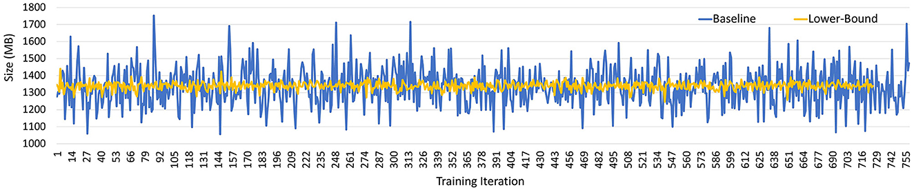
Figure 7. Karmarkar-Karp algorithm mini-batch size (MB) compared to baseline.

With a worst-case runtime of O(n), where n signifies the number of data points within the dataset, the Karmarkar-Karp algorithm emerges as a practical choice for handling extensive datasets. While not guaranteeing an optimal partition, it notably outperforms conventional greedy heuristics. However, employing the Karmarkar-Karp algorithm converges the dataset partition toward an optimal solution by minimizing the standard deviation between batches, thereby constraining variations and consequently the degree of freedom. This can leads to poor generalization of the model and a lower model accuracy at convergence. Furthermore, the Karmarkar-Karp algorithm is unideal for practical application is because the algorithm has high memory requirements and easily runs out of memory on the GPU. Therefore, our utilization of the Karmarkar-Karp algorithm serves as a lower-bound estimator to measure the GPU memory footprint for the previously proposed samplers.

The Karmarkar-Karp algorithm partitions the dataset into sets with sizes similar to the fixed batch size whereas the Pytorch sampler implementation requires every dataset partition is of a fixed batch size. Consequently in our implementation of the algorithm, we perform a post-partitioning steps, rectifying any batches that exceed or are less than the specified batch size. The corrective step involves removing random elements from the oversized batches and appending the elements to undersized batches, ensuring uniformity in batch size across the dataset.

3.2 Interquartile range (IQR) strategy

Interquartile Range (IQR) sampler—The Interquartile Range (IQR) method is based on the interquartile range and identifies outliers by measuring the spread of data between the first (Q1) and third (Q3) quartiles. Outliers are typically values below Q1 − 1.5*IQR or above Q3+1.5*IQR. In particular, IQR-based methods are proven to be robust in situations where the data deviates from normality and exhibits skewness (Iglewicz and Hoaglin, 1993). Given a skewed distribution, users can also adjust the outlier threshold value depending on the the dataset distribution. As our dataset is right-skewed dataset, we detect outliers using the upper bound equation,

$Q3+1.5*IQR$

After identifying outliers with the IQR method, we distribute each outlier to a different batch in a round-robin fashion. We hypothesize the IQR strategy will most effectively balance the outliers among the mini-batches due to the unconstrained degree of freedom, unlike the Karmarkar-Karp algorithm, allowing for shuffling of outliers. In particular, assigning graphs with varying sizes to a single mini-batch can include a more diverse set of particle types leading to better generalization during model training.

3.3 Distributed data parallel training

Data parallelism can harness an extensive training dataset and exploit a parallel High-Performance Computing (HPC) environment. A widely used parallelization strategy, is employing synchronous Stochastic Gradient Descent (SGD) with data parallelism (Zinkevich et al., 2010). In this data parallel training paradigm, workers are initialized with identical weight parameters, and mini-batches are evenly distributed among them. Each worker independently computes local gradients based on its assigned training samples. At the end of each iteration, these local gradients are averaged across all processes and broadcasted back via inter-process communication using an MPI Allreduce operation (Sergeev and Balso, 2018). Consequently, all workers can update their local model parameters with globally synchronized gradients. This strategy enables efficient parallel processing across multiple GPUs while maintaining synchronization through coordinated gradient updates, contributing to enhanced model training performance in the distributed HPC environment. Therefore, we incorporate a distributed data parallel (DDP) implementation for each of the proposed mini-batch balancing strategies.

Distributed Sampler—The Distributed Sampler class provided by Pytorch divides the full dataset into the number of subsets as there are processes launched during initialization. The subsets during local shuffling are partitioned using an interleaving pattern. We take the data subsets for each GPU device and implement a distributed version for each of the proposed mini-batch balancing strategies within each sampler. All of the strategies use local shuffling and keep the global batch size constant. Global batch size is calculated (number of devices * per-device batch size). In the context of this paper, we use the terms global batch size interchangeably with effective batch size. We also use the term local batch size interchangeably with the per-device batch size. We evaluate the effectiveness of these samplers in the distributed setting.

4 Performance evaluation

4.1 Experimental setup

The following tests have been run on the NERSC Perlmutter cluster. We use GPU-accelerated nodes on Perlmutter for our experiment. Each of the heterogeneous 1,536 nodes consist of 1 64-core AMD Milan CPU and 4 NVIDIA A100 GPUs using a 3-hop dragonfly topology interconnect. Each hardware-accelerated node also comes with 256 GB of DDR4 DRAM and 40 GB HBM for each GPU.

The Perlmutter storage system (also referred to as “Perlmutter Scratch”) uses an all-flash Lustre parallel filesystem (Leventhal, 2008). The system holds upto 35 PB of data, 16 metadata servers (MDS), 274 Object Storage Servers (OSS), 3,792 dual-ported NVMe SSDs, 1 OST, 1 OST, and 12 NVMes.

Software—For the codebase, we use the Torch Geometric library (Fey and Lenssen, 2019) for graph representation built on top of the PyTorch machine learning framework (Paszke et al., 2019) in addition to system-specific libraries built on top. To run our parallel and distributed framework we use the PyTorch Distributed Data Parallel (DDP) library. We also leverage mpi4py and h5py to access MPI and HDF5 library functions respectively, and NCCL (NVIDIA, 2023) for synchronizing the distributed model on NVIDIA GPU-based systems.

Datasets—LArTPC neutrino graph data is generated from simulated neutrino interactions publicly provided by the MicroBooNE project (Abratenko and Aldana, 2022b,a). The charge measurements (hits) from the detector represent the nodes of the graph. The tracks of the hits represent the edges of the graph. Three independent graphs are produced for each neutrino interaction corresponding to the three readout planes in the detector. The event graphs vary in size. The simulated neutrino data is comprised of 317,084 graphs in total and are split into 95% of samples for training (300,396 graphs), and 5% of samples for validation and testing (16,688 graphs). The total size of the dataset is 75 GB. The graph samples are stored in the Pytorch files where one file represents a graph sample. For the one file storing all samples, all training samples are stored in a single HDF5 file in which one graph sample corresponds to one HDF5 group. Each group contains feature vectors stored as HDF5 datasets.

We use the carefully generated subsets of the dataset, 1 and 10% of all samples. These datasets are created to show the performance of the proposed mini-batch balancing strategies on datasets of varying sizes. These graphs are chosen by selecting a continuous range of event IDs from the full dataset.

Evaluation metrics—In the evaluation of our GNN, we prioritize precision and recall as pivotal metrics over accuracy. Precision serves as an indicator of the accuracy of positive predictions, offering insights into the model's proficiency in correctly identifying instances of interest. On the other hand, recall evaluates the model's effectiveness in capturing all relevant instances within the dataset. Recall refers to the ratio of correctly predicted positive observations to the all observations in actual class. Consequently, we use primarily use recall over accuracy to measure performance.

Our primary objective is the classification of hits based on particle type. In this context, precision and recall are particularly pertinent metrics, as they provide a nuanced understanding of the model's performance in correctly identifying positive instances and ensuring comprehensive coverage of the relevant particle types. By emphasizing precision and recall in our evaluation, we aim to gain a more insightful and nuanced assessment of the GNN's capabilities, specifically tailored to the intricacies of particle type classification.

Model training—The baseline model training spans 80 epochs, a point where both precision and recall values converge, offering a stable assessment of model effectiveness. The application trains on the NuGraph2 model with a global batch size set at 64. In distributed setups, we leverage the Distributed Data Parallel (DDP) Framework and deploy one MPI process per GPU device. We ensure the effective batch size remains consistent by fixing the global batch size and reducing the local batch size accordingly. We use maximum reserved GPU memory (torch.cuda.max_memory_reserved()) provided by the Pytorch cache memory allocator to find the value of the maximum memory footprint on a given GPU device. To evaluate the proposed samplers, we use a threshold of recall improvement of more than 0.01 before stopping training to verify the model has converged.

4.2 Initialization overhead of mini-batch balancing strategies

We analyze the setup overhead for the mini-batch balancing strategies. The initialization time is a one-time preprocessing overhead during sampler initialization and batch creation takes place at the beginning of every epoch. Table 3 presents the overhead of strategy initialization and batch creation times. Of the presented strategies, the Karmarkar-Karp sampler runs into an OOM exception at initialization. As mentioned above, the Karmarkar-Karp algorithm has high memory requirements and therefore incurs an expensive initialization step prone to OOM exceptions for large datasets. This is also the case shown running the full dataset with the Karmarkar-Karp sampler. However, as observed in Table 4, the smaller-sized datasets do not run out of memory for the Karmarkar-Karp sampler. The results also show the remaining balancing strategies heavily outweigh the default random sampler in regards to initialization time and batch creation time. The initialization time for the IQR sampler is 900.7 times more expensive than the random sampler and the Z-score batch creation time is 4.24 times the time it takes to construct a batch for the random sampler. Furthermore, the initialization time and batch creation time grows proportionally to the size of the dataset for both the random and balancing strategies. These times also decrease proportionally with an increased number of GPUs.

Table 3

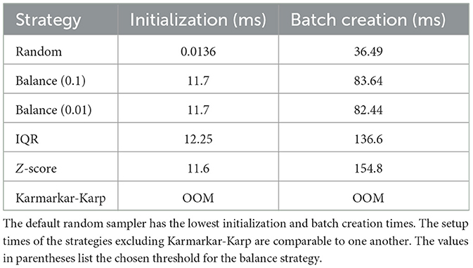
Table 3. The setup overhead for using different balancing strategies on the full dataset.

Table 4

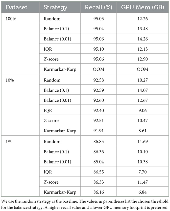
Table 4. Performance of datasets after model training.

However, the duration for running the complete dataset for one epoch is ~1 h and full training takes over 80 h. We also observe that both the initialization and batch creation times in Table 3 individually do not surpass 200 ms. Consequently, creating a batch at the start of each epoch consists of 0.005% of total epoch time and the one-time initialization cost takes up an even smaller fraction. Due to the nearly negligible setup overhead, we conclude that the overhead, constituted by the combined time spent on initialization and batch creation, is not significant in comparison to overall cost incurred during the model training process.

4.3 Balancing strategy performance on datasets

We highlight the effectiveness of various balancing strategies in reducing GPU memory footprint throughout the model convergence process. We use this experiment as a proof of concept to compare how the GPU memory footprint fares in comparison to the baseline GNN model used in real-world application for reconstructing low-level particles rather than using hyperparameters to induce an OOM error. Comparisons between different balancing strategies are conducted using the random strategy as a baseline. The random strategy assigns graph samples to batches randomly, while balancing strategies aim to distribute samples to different mini-batches according to the graph sample size. The maximum GPU memory footprint is monitored during training, and the results are summarized in Figure 8 and the rightmost column of Table 4.

Figure 8

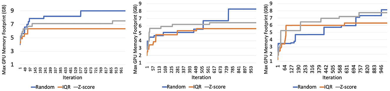
Figure 8. Memory consumption of 2, 4, and 8 GPUs, respectively.

Each of the datasets we test the strategy on has the same distribution but a varying range of sample sizes. The baseline random sampler achieves recall values of 95, 92.6, and 86.9% on the 100, 10, and 1% datasets, respectively as shown in Figure 9. As dataset size decreases, both baseline and balancing strategies exhibit declining recall values. However, the decrease is more pronounced for the balancing strategies. While all balance strategies outperform or match the baseline on the full dataset, the number of strategies performing similarly diminishes with smaller datasets. This result implies a tradeoff between the size of the dataset and model recall. As the dataset size decreases, the recall value achieved after validation loss converges also decreases.

Figure 9

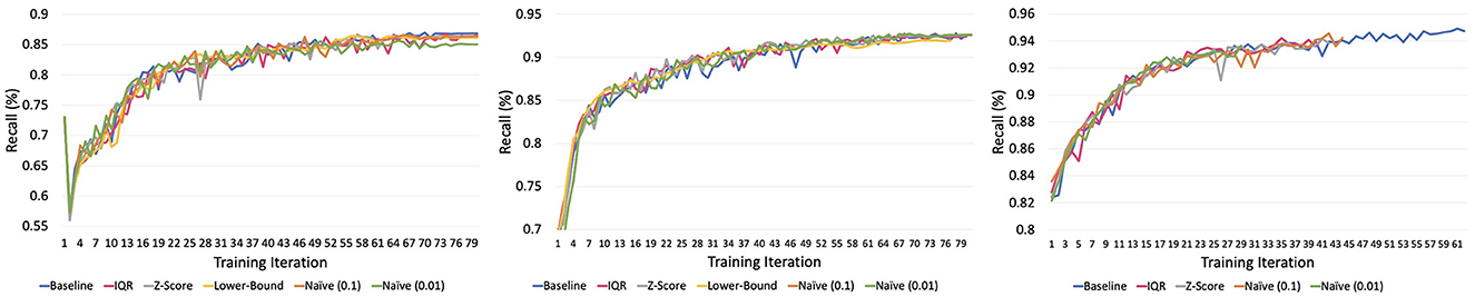
Figure 9. Recall values for 1, 10, and 100% datasets, respectively.

Analyzing the results in Table 4, we also identify a tradeoff between GPU memory footprint and recall values for the Karmarkar-Karp strategy. The Karmarkar-Karp sampler, serving as a theoretical lower-bound for GPU memory footprint, consistently exhibits the lowest recall values across all datasets. This implies a positive correlation between a higher degree of freedom and improved recall.

The post-launch assessment of the balance sampler exhibited inferior performance compared to the random sampler. In the experiment, the balance sampler tests two different user-specified thresholds to determine the fraction of outliers to distribute between batches. Regardless of the treated fraction of the dataset as outliers, the maximum GPU memory footprint surpassed that of the random sampler. This observation highlights the lesson that utilization of a dataset fraction for outlier distribution can expedite OOM issues rather than alleviating them.

Focusing on the IQR sampler, which consistently achieves the lowest GPU memory footprint, we note that recall falls below baseline recall for the 1 and 10% dataset subsets. However, for the full dataset, accuracy is comparable to the baseline. We attribute this to the IQR strategy's threshold settings, which impose more restrictions on subsets, leading to increased accuracy as dataset size grows and the impact of partitioning outliers decreases.

4.4 Scalability of balancing strategies

We scale up the HEP application by decreasing the local batch size and keeping the effective batch size constant when increasing the number of GPUs used for training. This multi-GPU implementation of the application increases the aggregate GPU memory size of the entire application. However, drastically reducing the local batch size can detriment the recall accuracy whereas too large of a batch size can cause an OOM exception. Therefore, we run our experiments using a moderate number of GPUs.

The strategies for balancing mini-batches demonstrate effective scalability, as evidenced by the evaluation of the top-performing strategies, namely IQR and Z-score, in comparison with the baseline. To emphasize the performance over an extended duration, we present the maximum GPU memory footprint in our experiments. Our experiments showcase results for configurations with 1, 2, 4, and 8 GPUs.

The IQR strategy distinguishes itself by consistently maintaining the maximum GPU memory footprint value for an extended period. This characteristic suggests that subsequent batch sizes, after reaching the maximum value, either remain the same or decrease in size. As illustrated in Table 5, all configurations consistently demonstrate that the IQR strategy outperforms others, achieving up to a 32% reduction in memory usage in the 4-GPU configuration. In contrast, the baseline random sampler exhibits the highest GPU usage over time. These findings imply the efficacy of the IQR strategy in memory reduction, particularly in multi-GPU configurations. Furthermore, applying the IQR strategy to our HEP workflow for multiple GPUs allows us to avoid the OOM exception.

Table 5

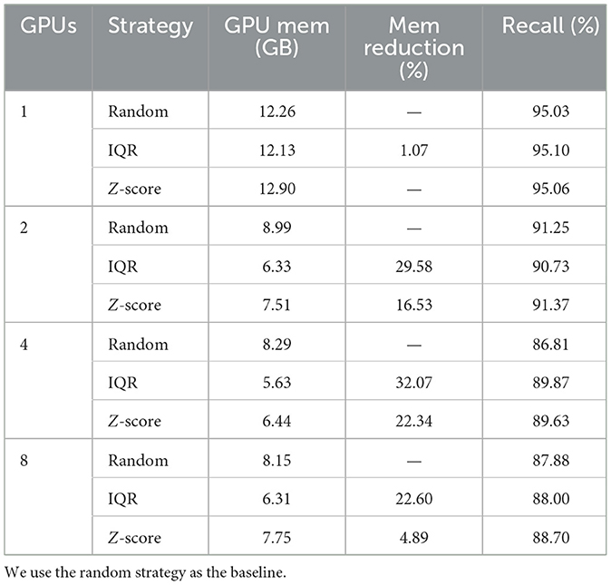
Table 5. Performance of datasets on upto 8 GPUs using the top-performing strategies.

5 Conclusion

The out-of-memory (OOM) exception frequently arises in GNN applications dealing with expansive datasets, particularly when the size of these datasets exceed GPU memory capacity. This problem is made more apparent running larger datasets on HPC systems. In this paper we aim to mitigate high GPU memory usage in training large-scale GNNs. To address this challenge, we present a multiple workload balancing strategies, crucial for managing independent graph samples with varying sizes. By evaluating the performance of these strategies as data loading samplers on multiple datasets, we can observe the effectiveness of each strategy on both a single-GPU and distributed setting. Our experiments using datasets of various sizes and multiple GPU devices extends the potential applicability of our work to different GNN applications using input datasets with irregular graph sizes. The results presented in this paper give researchers the insight of selecting the most appropriate balancing scheme for their application.

Data availability statement

The original contributions presented in the study are included in the article/supplementary material, further inquiries can be directed to the corresponding author.

Author contributions

CL: Conceptualization, Data curation, Formal analysis, Investigation, Methodology, Software, Validation, Visualization, Writing – original draft, Writing – review & editing. VH: Methodology, Software, Supervision, Validation, Writing – review & editing. GC: Funding acquisition, Supervision, Validation, Writing – review & editing. KW: Methodology, Validation, Writing – review & editing. AAu: Supervision, Validation, Writing – review & editing. AAg: Funding acquisition, Supervision, Writing – review & editing. AC: Funding acquisition, Supervision, Writing – review & editing. W-KL: Conceptualization, Funding acquisition, Investigation, Methodology, Project administration, Resources, Supervision, Validation, Writing – original draft, Writing – review & editing.

Funding

The author(s) declare financial support was received for the research, authorship, and/or publication of this article. This material is based upon work supported by the U.S. Department of Energy, Office of Science, Office of Advanced Scientific Computing Research, Scientific Discovery through Advanced Computing (SciDAC) program under Award Number DE-SC0021399, grant ‘HEP Data Analytics on HPC', No. 1013935, and the Office of High Energy Physics (CompHEP-Exa.trkx) under Contract No. DE-AC02-07CH11359. Partial support was also acknowledged from NIST award 70NANB19H005 and NSF award OAC-2331329. We acknowledge the MicroBooNE Collaboration for making publicly available the datasets (Abratenko and Aldana, 2022b,a) employed in this work. These data sets consist of simulated neutrino interactions from the Booster Neutrino Beamline overlaid on top of cosmic ray data collected with the MicroBooNE detector (Acciarri and et. al, 2017). This research used resources of the National Energy Research Scientific Computing Center, a DOE Office of Science User Facility supported by the Office of Science of the U.S. Department of Energy under Contract No. DE-AC02-05CH11231 using NERSC award ASCR-ERCAP0028620. This work was partially supported by the National Institute of Standards and Technology award number 70NANB19H005. This work was also supported by the National Science Foundation Graduate Research Fellowship under Grant No. DGE-2039655.

Conflict of interest

The authors declare that the research was conducted in the absence of any commercial or financial relationships that could be construed as a potential conflict of interest.

Publisher's note

All claims expressed in this article are solely those of the authors and do not necessarily represent those of their affiliated organizations, or those of the publisher, the editors and the reviewers. Any product that may be evaluated in this article, or claim that may be made by its manufacturer, is not guaranteed or endorsed by the publisher.

References

Abi, B., and Acciarri, R. (2020). Deep Underground Neutrino Experiment (DUNE), Far Detector Technical Design Report, Volume I: Introduction to DUNE.

Google Scholar

Abratenko, P., and Aldana, A. (2022a). MicroBooNE BNB Electron Neutrino Overlay Sample (No Wire Info).

Google Scholar

Abratenko, P., and Aldana, A. (2022b). MicroBooNE BNB Inclusive Overlay Sample (With Wire Info).

Google Scholar

Acciarri, R., Adams, C., An, R., Aparico, A., Aponte, S., Asaadi, J., et al. (2017). Design and construction of the microboone detector. J. Instr. 12:P02017. doi: 10.1088/1748-0221/12/02/p02017

Crossref Full Text | Google Scholar

Anonymous (2003). Lustre : A Scalable, High-Performance File System. Cluster File Systems Inc. white paper, version 1.0. Available at: http://www.lustre.org/docs/whitepaper.pdf

Google Scholar

ExaTrkX Collaboration (2024). ExaTrkX: Exascale Tracking for High Energy Physics. Available at: https://exatrkx.github.io/ (accessed August 31, 2024).

PubMed Abstract | Google Scholar

Fey, M., and Lenssen, J. E. (2019). Fast graph representation learning with PyTorch geometric. CoRR abs/1903.02428. doi: 10.48550/arXiv.1903.02428

Crossref Full Text | Google Scholar

Gao, Y., Liu, Y., Zhang, H., Li, Z., Zhu, Y., Lin, H., et al. (2020). “Estimating GPU memory consumption of deep learning models,” in Proceedings of the 28th ACM Joint Meeting on European Software Engineering Conference and Symposium on the Foundations of Software Engineering, ESEC/FSE 2020 (New York, NY: Association for Computing Machinery), 1342–1352.

PubMed Abstract | Google Scholar

Hewes, V., and Aurisano, A. (2021). Graph neural network for object reconstruction in liquid argon time projection chambers. EPJ Web Conf. 251:e03054. doi: 10.1051/epjconf/202125103054

PubMed Abstract | Crossref Full Text | Google Scholar

Hu, W., Fey, M., Ren, H., Nakata, M., Dong, Y., and Leskovec, J. (2021). “OGB-LSC: a large-scale challenge for machine learning on graphs,” in Thirty-fifth Conference on Neural Information Processing Systems Datasets and Benchmarks Track (Round 2) (NIPS).

Google Scholar

Iglewicz, B., and Hoaglin, D. (1993), “Volume 16: how to detect handle outliers”, in The ASQC Basic References in Quality Control: Statistical Techniques, ed. E. F. Mykytka. Available at: https://www.semanticscholar.org/paper/Volume-16%3A-How-to-Detect-and-Handle-Outliers-Hoaglin/d524a172b49e25f888376d662ee364aa77d99e8a

PubMed Abstract | Google Scholar

Jia, Z., Kwon, Y., Shipman, G., McCormick, P., Erez, M., and Aiken, A. (2017). A distributed multi-GPU system for fast graph processing. Proc. VLDB Endow. 11, 297–310. doi: 10.14778/3157794.3157799

Crossref Full Text | Google Scholar

Ju, X., Murnane, D., Calafiura, P., Choma, N., Conlon, S., Farrell, S., et al. (2021). Performance of a geometric deep learning pipeline for Hl-lHC particle tracking. The Eur. Phys. J. C 81:8. doi: 10.1140/epjc/s10052-021-09675-8

Crossref Full Text | Google Scholar

Karmarkar, N. (1984). “A new polynomial-time algorithm for linear programming,” in Proceedings of the Sixteenth Annual ACM Symposium on Theory of Computing, STOC '84 (New York, NY: Association for Computing Machinery), 302–311.

Google Scholar

Korf, R. E. (1998). A complete anytime algorithm for number partitioning. Artif. Intell. 106, 181–203. doi: 10.1016/S0004-3702(98)00086-1

Crossref Full Text | Google Scholar

Lee, C. S., Hewes, V., Cerati, G., Kowalkowski, J., Aurisano, A., Agrawal, A., et al. (2023). “A case study of data management challenges presented in large-scale machine learning workflows,” in 2023 IEEE/ACM 23rd International Symposium on Cluster, Cloud and Internet Computing (CCGrid) (Bangalore), 71–81. doi: 10.1109/CCGrid57682.2023.00017453

Crossref Full Text | Google Scholar

Leventhal, A. (2008). Flash storage today: can flash memory become the foundation for a new tier in the storage hierarchy? Queue 6, 24–30. doi: 10.1145/1413254.1413262

Crossref Full Text | Google Scholar

National Energy Research Scientific Computing Center (NERSC) (2024). High-Performance Computing Resources. Lawrence Berkeley National Laboratory. Available at: https://www.nersc.gov/ (accessed August 31, 2024).

Google Scholar

Nguyen, T. T., Trahay, F., Domke, J., Drozd, A., Vatai, E., Liao, J., et al. (2022). “Why globally re-shuffle? revisiting data shuffling in large scale deep learning,” in 2022 IEEE International Parallel and Distributed Processing Symposium (IPDPS), 1085–1096. doi: 10.1109/IPDPS53621.2022.00109

Crossref Full Text | Google Scholar

NVIDIA (2023). NVIDIA Collective Communications Library (NCCL). Available at: https://developer.nvidia.com/nccl (accessed August 31, 2024).

Google Scholar

Paszke, A., Gross, S., Massa, F., Lerer, A., Bradbury, J., Chanan, G., et al. (2019). Pytorch: an imperative style, high-performance deep learning library. CoRR, abs/1912.01703. doi: 10.48550/arXiv.1912.01703

Crossref Full Text | Google Scholar

Peng, C., Xiao, T., Li, Z., Jiang, Y., Zhang, X., Jia, K., et al. (2017). MegDet: a large mini-batch object detector. CoRR, abs/1711.07240. doi: 10.48550/arXiv.1711.07240

Crossref Full Text | Google Scholar

Pumma, S., Si, M., Feng, W.-C., and Balaji, P. (2019). Scalable deep learning via i/o analysis and optimization. ACM Trans. Parallel Comput. 6, 1–34. doi: 10.1145/3331526

PubMed Abstract | Crossref Full Text | Google Scholar

Rajbhandari, S., and Ruwase, O. (2021). “Zero-infinity: breaking the GPU memory wall for extreme scale deep learning,” in Proceedings of the International Conference for High Performance Computing, Networking, Storage and Analysis, SC '21. New York, NY: Association for Computing Machinery.

Google Scholar

Sergeev, A., and Balso, M. D. (2018). Horovod: fast and easy distributed deep learning in Tensorflow. arXiv [Preprint]. arXiv:1802.05799.

Google Scholar

Tripathy, A., Yelick, K., and Buluc, A. (2020). “Reducing communication in graph neural network training,” in Proceedings of the International Conference for High Performance Computing, Networking, Storage and Analysis (SC) (Atlanta, GA), 987–1000.

Google Scholar

Yang, S., Zhang, M., Dong, W., and Li, D. (2023). “Betty: enabling large-scale GNN training with batch-level graph partitioning,” in Proceedings of the 28th ACM International Conference on Architectural Support for Programming Languages and Operating Systems, Volume 2, ASPLOS 2023 (New York, NY: Association for Computing Machinery), 103–117.

Google Scholar

Zhu, R., Zhao, K., Yang, H., Lin, W., Zhou, C., Ai, B., et al. (2019). Aligraph: A Comprehensive Graph Neural Network Platform. Proc. VLDB Endowm. 12, 2094–2105. doi: 10.14778/3352063.3352127

Crossref Full Text | Google Scholar

Zinkevich, M. A., Weimer, M., Smola, A., and Li, L. (2010). “Parallelized stochastic gradient descent,” in Proceedings of the 23rd International Conference on Neural Information Processing Systems—Volume 2, NIPS'10 (Red Hook, NY: Curran Associates Inc), 2595–2603.

Google Scholar