Nek5000/RS performance on advanced GPU architectures

The authors explore performance scalability of the open-source thermal-fluids code, NekRS, on the U.S. Department of Energy's leadership computers, Crusher, Frontier, Summit, Perlmutter, and Polaris. Particular attention is given to analyzing performance and time-to-solution at the strong-scale limit for a target efficiency of 80%, which is typical for production runs on the DOE's high-performance computing systems. Several examples of anomalous behavior are also discussed and analyzed.

1 Introduction

As part of its Exascale Computing Project, the U.S. Department of Energy has deployed a sequence of platforms at its leadership computing facilities leading up to those capable of reaching > 1 exaFLOPS (10¹⁸ floating point operations per second). These highly parallel computers feature ≈10³–10⁴ nodes, each equipped with powerful CPUs and anywhere from 4 to 12 accelerators (i.e., GPUs), which provide the bulk of the compute power. For reasons of efficiency, a favored programming model for these architectures is to assign a single process (i.e., MPI rank) to each GPU (or GPU processing unit, such as a GCD on the AMD MI250X or a tile on the Intel PVC) and to execute across the accelerators using a private distributed-memory programming model. With P = 10³–10⁵ MPI ranks, this approach affords a significant amount of internode parallelism and contention-free bandwidth with no increase in memory-access latency, save for the relatively sparse internode communication that is handled by MPI.

Here, we explore parallel scalability for the open source thermal-fluids simulation code Nek5000/RS (Fischer et al., 2008, 2022, 2021) on serveral of these high-performance computing (HPC) platforms. Computational scientists engaged in HPC are typically interested in reducing simulation campaign times that can take days, weeks, or months to hours, days, or weeks. At runtime, these performance gains are realizable by increasing the number of compute units assigned to the task at hand, provided that order-unity parallel efficiency is sustained for the target values of P. The purpose of the present study is to characterize parallel efficiency of DOE's exascale and pre-exascale platforms as a function of problem size, n, and process count, P. An important measure is the local problem size, n/P required to sustain a parallel efficiency of η_P = 0.8. We denote this value of n/P as n_0.8 (the precise value of η_P = 0.8 is somewhat arbitrary but is not atypical for production campaigns).

The baseline simulation code used for this study is NekRS, which is the GPU-oriented version of Nek5000. NekRS was developed as part of the Center for Efficient Exascale Discretizations (CEED), supported by the U.S. Department of Energy's Exascale Computing Project (ECP). We expect that many of the scalability findings herein will be similar to those realized by other HPC codes that are based on partial differential equations (PDEs). For example, Fischer et al. (2020) found that deal.ii (Arndt et al., 2017), MFEM (Anderson et al., 2020), and Nek5000 had similar performance characteristics over a suite of benchmark problems on Argonne's CPU-based IBM BG/Q, Cetus.

1.1 Code overview

Nek5000/RS is based on the spectral element method (SEM) (Patera, 1984). The SEM uses Nth-order tensor-product polynomials in the reference domain, $\widehat{\Omega }$ := [−1, 1]³. Use of nodal bases situated at the Gauss-Lobatto-Legendre quadrature points provides numerical stability as well as convenient and highly accurate numerical quadrature, which largely obviates the need for interpolation to alternative quadrature points, save for evaluation of the advection term, where accurate integration is required to preserve skew-symmetry, as noted in Malm et al. (2013). To handle complex geometries, the computational domain Ω is partitioned into E nonoverlapping elements, Ω^e, e = 1, …, E, each of which is a mapped image of $\widehat{\Omega }$. Tensor-product-sum factorization allows for efficient matrix-free operator evaluation in $\widehat{\Omega }$ with only O(n) memory references and O(nN) BLAS3-type (tensor-contraction) operations, where the number of grid points is n≈EN³ (Deville et al., 2002; Orszag, 1980). Semi-implicit timestepping is used to advance the unsteady incompressible Navier-Stokes equations (and other physical processes such as thermal transport and combustion, which we do not address here).

The Navier-Stokes time-advancement involves three principal substeps to update the vector velocity field, u^m, and pressure, p^m, at time t^m. Omitting details of boundary conditions and constants, the first step amounts to gathering known data, including explicit treatment of the nonlinear advection terms,

$\begin{array}{llll}\widehat{\text{u}}& =& {\displaystyle \sum _{j=1}^k}{\beta }_j{\text{u}}^{m-j}-\Delta t{\alpha }_j{NL}^{m-j},& (1)\end{array}$

where the β_js and α_js are order-unity coefficients associated with respective kth-order backward-difference and extrapolation formulas. Evaluation of the advection term, NL^m−j, is compute intensive because it is evaluated using overintegration with a 3/2s-rule to ensure numerical stability (Malm et al., 2013). The explicit update (Equation 1) leads to a Courant-Friedrichs-Lewy (CFL) limit on the stepsize of CFL := $\underset{x_i\in \Omega }{max}\frac{\Delta t\left|u_i\right|}{\Delta x_i}\approx 0.5$. To circumvent this constraint, a frequently used alternative in Nek5000/RS is the characteristics based formulation of Maday et al. (1990) and Patel et al. (2019),

$\begin{array}{llll}\widehat{\text{u}}& =& {\displaystyle \sum _{j=1}^k}{\beta }_j{\tilde{\text{u}}}^{m-j},& (2)\end{array}$

where ${\tilde{\text{u}}}^{m-j}:=\tilde{\text{u}}(\text{x},t^m)$ and $\tilde{\text{u}}(\text{x},t)$ satisfies

$\begin{array}{ll}{\tilde{\text{u}}}_t=-\text{u}·\nabla \tilde{\text{u}}(\text{x},t),\text{x}\in \Omega ,t\in \left[t^{m-j},t^m\right],& (3)\end{array}$

with initial condition $\tilde{\text{u}}(\text{x},t^{m-j})={\text{u}}^{m-j}(\text{x})$. For CFL ≈2S, solution of Equation 3 requires 4Sk nonlinear evaluations per timestep, Δt, where S = 1 or 2 are typical numbers of subcycle steps, and k is the temporal order of accuracy. With k = 2 and S = 1 the advection update (Equations 2, 3) can account for ≈30% of the runtime and a significant fraction of the flops.

The second Navier-Stokes step is the pressure Poisson solve,

$\begin{array}{llll}-{\nabla }^2{p}^m& =& \frac{1}{\Delta t}\nabla ·\widehat{\text{u}}& (4)\end{array}$

This step uses GMRES, preconditioned by FP32 p-multigrid with overlapping Schwarz smoothers. Each Schwarz subdomain consists of a single spectral element with additional degrees-of-freedom lifted from neighboring elements. The local subdomain problems are solved using a fast diagonalization method that is implemented as a sequence of tensor contractions, ${\overline{\underset{\_}{p}}}^e=(S_{\zeta }\otimes S_{\eta }\otimes S_{\xi })D^{-1}(S_{\zeta }^T\otimes S_{\eta }^T\otimes S_{\xi }^T){\overline{\underset{\_}{f}}}^e,$ e = 1, …, E, where D is a diagonal matrix of eigenvalues, S_* is the matrix of eigenvectors for the 1D Poisson operator in each coordinate (ξ, η, ζ) in an extended reference element, $\overline{\Omega }$, and ${\overline{\underset{\_}{u}}}^e$ and ${\overline{\underset{\_}{f}}}^e$ are respective solutions and data in the extended subdomain, ${\bar{\Omega }}^e$. The lowest level of the p-multigrid entails applying one or two V-cycles of algebraic multigrid with Hypre to a coarse-grid problem based on the spectral element vertices. Overall, the pressure solve is communication intensive because of the long tails of the Green's functions associated with the Poisson operator.

The final Navier-Stokes update entails solving a diagonally-dominant Helmholtz system for the velocity components,

$\begin{array}{llll}\text{H}{\text{u}}^m& =& \widehat{\text{u}}-\Delta t\nabla p^m,& (5)\end{array}$

where H := $-\frac{\Delta t}{Re}{\nabla }^2+{\beta }_0\text{I}$, represents the update of the momentum equation with the implicitly treated viscous terms. Iterative solution of the block system H updates all velocity components simultaneously, which reduces the number of message exchanges by a factor of three in the Jacobi-preconditioned conjugate gradient solver and therefore amortizes communication latency.

Parallel-work decomposition is realized by partitioning the set of elements into contiguous subsets using recursive spectral bisection (Pothen et al., 1990) with load-balanced partitioning such that the number of elements per subdomain (i.e., per MPI rank) differs by at most 1. Given that we typically have several thousand spectral elements per GPU, load balance is not a source of inefficiency in production simulations.

For portability, all the GPU kernels are written in OCCA (Medina et al., 2014; OCCA, 2021), which was developed by Tim Warburton's group at Virginia Tech. and Rice University. Many of the high-performance kernels originated with the libParanumal library (Chalmers et al., 2020), also developed by Warburton's group. Roofline performance and scaling results can be found in the Hipbone study of Chalmers et al. (2023) and the NekRS study (Min et al., 2022). In the latter, which includes detail NVIDIA Nsight timing data, the authors note that all kernels in NekRS, save for the latency-bound gather-scatter kernels in the coarse p-multigrid levels, achieve near-roofline performance defined as > 70 % of the leading-performance limiter. Additional details of the NekRS GPU implementation, including kernel pseudocode, can be found in Fischer et al. (2022).

1.2 Performance metrics

A primary concern for computational scientists is the speed that can be realized for a particular application for a given architecture (here, an application is a particular problem that uses Nek5000/RS, which is an application code). For example, one frequently needs to estimate the number of node-hours and number of wall-clock hours that might be required for a large simulation campaign. A common metric, which is very much case-specific, is the number of degrees of freedom (dofs) per second that can be realized on a platform, or perhaps the number of dofs per second per accelerator (i.e., per MPI rank¹). In the sequel, we will assign GDOFS to the quantity “billions of dofs per second per rank.” The case-specificity aspect of GDOFS is that one can realize a much larger GDOFS value for linear solution of Ax = b than would be possible for, say, a single timestep of an incompressible Navier–Stokes solver.

Despite the large variance in GDOFS from one problem class to the next, it is nonetheless a worthy metric when making platform-to-platform comparisons. A related metric is the time-to-solution or, in the case of a timestepping simulation code that could take an arbitrarily large number of steps, the time per step, t_step, ² which we measure in seconds. Even for a given code and architecture this latter quantity is subject to significant variability because some problems or computational meshes are more ill-conditioned than others, which leads to higher iteration counts in the linear solvers (e.g., in the pressure solve for an incompressible flow simulation) and hence a longer time per step.

GDOFS and t_step are dependent, or output, parameters. For a fixed platform, code, and problem, users still have two independent parameters at their disposal: n, the problem size or number of dofs,³ and P, the number of ranks (here, accelerator devices) to use. For a fixed problem size, n (which is determined by resolution requirements), there is only one variable, namely, P. A user who is contemplating a simulation campaign will often be interested in predicting performance over a range of n. Under the given conditions, we will see that the most important performance predictor is

$\begin{array}{llll}\frac{n}{P}& =& \text{the number of grid points per device},& (6)\end{array}$

where we reiterate that we are assigning a single MPI rank to each device.

Two other dependent quantities of interest are parallel efficiency, η_P, and realized FLOPS, the measurable number of 64-bit floating-point operations per second. We typically will report FLOPS per rank, which is more universal than aggregate FLOPS. Also, in cases where mixed precision is used (e.g., when 32-bit arithmetic is used in a preconditioner), we count the FP32 flops as a half-flop each. A typical definition of (strong-scaling) parallel efficiency is

$\begin{array}{llll}{\eta }_P& :=& \frac{P_0{t}_{step}(P_0)}{P{t}_{step}(P)}=\frac{\text{GDOFS}(P)}{\text{GDOFS}(P_0)},& (7)\end{array}$

where t_step(P) is the time per step when running a fixed problem of fixed size, n, on P ranks and GDOFS(P) is the corresponding number of gigadofs per second per rank. Here, P₀ is the smallest number of ranks that is able to hold the problem. On some architectures, the amount of memory per GPU is relatively small, which prevents extensive strong-scaling studies (from a user's perspective, however, this is potentially a happy circumstance since there is “just enough” memory and not a lot of idle memory that incurs unnecessary capital and power overhead).

An alternative definition of parallel efficiency is given by the relationship

$\begin{array}{llll}{S}_P& =& {\eta }_{P}P{S}_1.& (8)\end{array}$

Here, S_P is the speed on P processors, which could be measured in total (not per rank) FLOPS or GDOFS. This definition is equivalent to Equation 7 when P₀ = 1. The utility of this definition is that one can consider it for either weak- (fixed n/P) or strong- (fixed n) scaling studies. If FLOPS are used, it is relatively easy to get FLOPS on one rank for a smaller version of the application problem (although that might not be a useful starting point in the exascale era given that no exascale problem comes anywhere close to fitting on one rank).

What Equation 8 tells us is that the speed on P ranks should be ≈P times the speed on 1 rank, provided we can sustain close to unity efficiency, η_P≈1. We remark that HPC users generally want to run as fast as possible, particularly for large campaigns, so they want P≫1. However, they also need to efficiently use their allocation, which implies η_P≈1. This latter condition places a constraint on time-to-solution that is generally stronger than the unconstrained “min-time-to-solution” result. In our studies we will assume that the user is willing to run at 80% parallel efficiency, η_P = 0.8. Of course, other target efficiencies are possible, and a user can change P and, hence, η_P on a submission-by-submission basis for each case run in a given campaign. However, η_P = 0.8 is a reasonable starting point for analysis.

The first analysis question we address is, For a fixed problem size n, how many ranks can we use before η_P < 0.8? An accompanying question is, What is the time per step at that value? Users and developers are also interested in the cause of the departure from unity efficiency. For example, is it load imbalance? Message-passing overhead? Or lack of parallelism on the accelerator? In our examples, as is the case for Nek5000/RS in practice, load imbalance will not be a leading contributor to inefficiency as the work is sufficiently fine-grained such that it can be distributed in a balanced way across all ranks.

The key to the first question about number of ranks is to recognize that parallel efficiency typically drops as the local amount of work, n/P tends toward zero. So, fixing η_P = 0.8 implies n/P is a fixed value (for a given fixed-sized problem with P varying). We denote this value as n_0.8. It is the number of points per rank where the application realizes 80% efficiency, which is where we anticipate that users will typically run. For a given problem size, n,

$\begin{array}{ll}{n}_{0.8}:=\frac{n}{P}\text{such that }{\eta }_P=0.8.& (9)\end{array}$

With this definition, we can address the question of the expected t_step under these conditions. Assume that a given problem requires a certain amount of work, W, that is measured in total number of floating-point operations (FLOPS). Usually, W~Cn, where C is an n-independent constant, which implies that, to leading order, the amount of work scales with n. On P processors, we therefore expect

$\begin{array}{ll}{t}_{step}=\frac{W}{S_P}=\frac{Cn}{{\eta }_{P}P{S}_1}.& (10)\end{array}$

We define t_0.8 to be the value of t_step at 80% efficiency,

$\begin{array}{ll}{t}_{0.8}=\frac{C}{0.8}\frac{n/P}{S_1}.=\left(\frac{C}{0.8}\right)\frac{n_{0.8}}{S_1}.& (11)\end{array}$

We note that Equations 10, 11 are predicated on η_P being strongly dependent on (n/P) with no direct P dependence. There are times when there is a weak P dependence, particularly for P>10⁴. In this case, one can simply modify the analysis to have a P-dependent n_0.8.

We see from Equation 11 that the time per step is governed by the speed on a single rank, S₁ (larger is better), and the amount of work on a single rank, n_0.8 (smaller is better), where 80% efficiency is realized. If a new platform comes out with a 2 × increase in S₁ but a 4 × increase in n_0.8, then the net time-to-solution increases by 2 × . In HPC, it is the ratio, n_0.8/S₁, that is critical to fast time-to-solution. Much of this analysis can be found in Fischer et al. (2015, 2020). Communication overhead on GPU-based architectures is discussed in Bienz et al. (2021).

A typical use case for Equation 11 is that a user knows n, which is the number of gridpoints required to resolve a given simulation, and wants to know how many processors will be required to efficiently solve this problem and how long it will take to execute. The user also knows n_0.8 from scaling studies of the type provided here. From that, one can determine

$\begin{array}{ll}{P}_{0.8}=\frac{n}{n_{0.8}},& (12)\end{array}$

which is the maximum number of ranks that can be employed while sustaining 80% efficiency. The time per step will be t_0.8, and the total required node-hours will be

$\begin{array}{ll}\text{node hours}\approx \frac{P_{0.8}}{\text{ranks-per-node}}\times \frac{N_{steps}{t}_{0.8}}{3600\text{s/hour}},& (13)\end{array}$

where N_steps is the estimated number of timesteps.

1.3 Test cases

In the following sections we characterize these relevant parameters for NekRS across several of DOE's pre-exascale and exascale platforms, including Frontier, Crusher, Polaris, Perlmutter, ThetaGPU, and Summit. The principals from this list are described in Table 1. Simulations are performed using ExaSMR's 17 × 17 rod-bundle geometry, illustrated in Figure 1. This geometry is periodic in the axial flow direction, which allows us to weak-scale the problem by adding more layers of elements in the z direction (the model problem is essentially homogeneous in z). Each case starts with a pseudo-turbulent initial condition so that the iterative solvers, which compute only the change in the solution on each step, are not working on void solutions. Most of the cases are run under precisely the same conditions of timestep size, iteration tolerances, and averaging procedures, which are provided case by case in the sequel.

Table 1

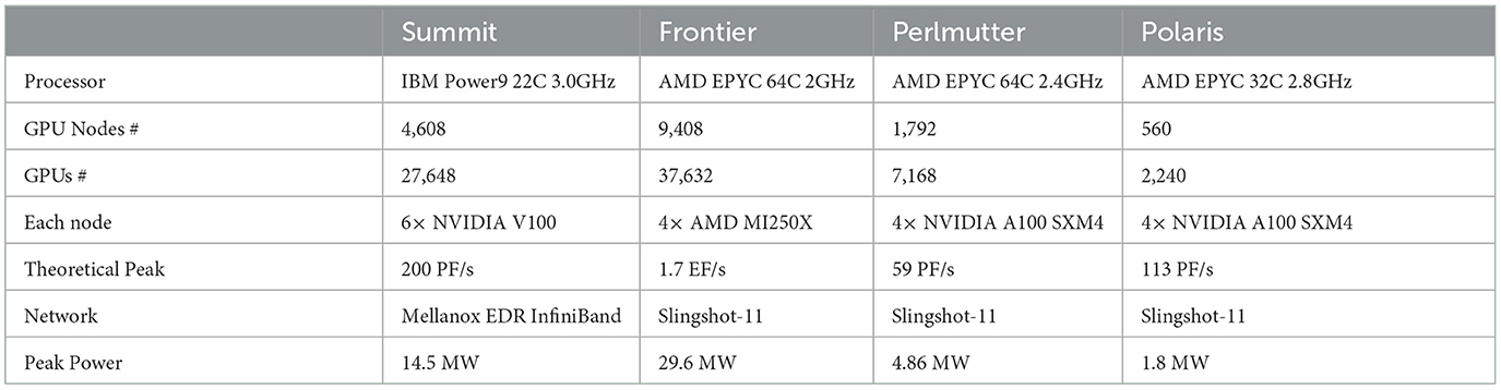
Table 1. Systems overview.

Figure 1

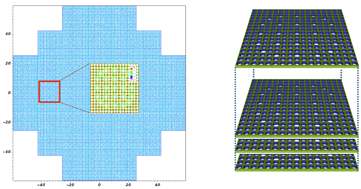
Figure 1. ExaSMR full-core configuration on the left and a single 17 × 17 rod bundle on the right.

We remark that the following performance summaries are for full Navier–Stokes solution times. We present a few plots that reflect work in salient kernels, such as the advection operator, which is largely communication-free, and the pressure-Poisson coarse-grid solve, which is highly communication-intensive. Detailed kernel-by-kernel breakdowns are presented in Fischer et al. (2022) and Min et al. (2022) and are available in every logfile generated by NekRS.

Further, we note that NekRS supports multiple versions of each of its high-intensity kernels and communication utilities. At runtime, NekRS selects the fastest kernel by running a small suite of tests for each invocation of the given utility. that particular kernel for the particular platform for the particular application. An example of these outputs, along with the kernel-by-kernel breakdown, is presented in Section 5.

1.4 Additional scaling studies

There have been multiple performance studies on GPUs that are relevant to the high-order methods used in the current work. Bienz et al. (2021) explored communication characteristics for the NVIDIA V100-based platforms, Summit (using Spectrum MPI) and Lassen (using MVAPICH). Kronbichler and Ljungkvist (2019) study the performance of matrix-free p-type finite element methods (FEMs) in deal.ii on several CPU and GPU architectures, including a single NVIDIA P100, where they observe 80% efficiency for n_0.8≈ 3–4 × 10⁵ when evaluating matrix-vector products. A more recent study, Kronbichler et al. (2023), demonstrates that deal.ii realizes 80% efficiency for Jacobi PCG on a single NVIDIA V100 when n_0.8≈ 3–4 × 10⁵. The same paper explores alternative PCG formulations to provide better data caching with fewer vector reductions on both CPUs and GPUs. Multi-GPU throughput studies presented in Vargas et al. (2022) reveal that MFEM needs n_0.8≈0.75–1.0 M points per V100 for single-node (P = 4) hydrodynamics simulations on LLNL's Sierra platform. For P = 64 V100s on LLNL's Lassen, the MFEM mini-app Laghos has n_0.8≈2M. The observed increase is expected at higher node counts because of MPI overhead. Sathyanarayana et al. (2025) find n_0.8≈ 2–4 M for finite-difference based WENO schemes when running on single NVIDIA A100s and AMD MI250X GCDs. Chalmers et al. (2023) provide in-depth performance analysis of high-order matrix-free kernel performance, including roofline models and throughput scaling on NVIDIA V100, AMD MI100, and AMD MI250X accelerators, all of which is of direct relevance to NekRS, which uses many of the same kernels.

2 NekRS performance on a single GPU

Table 2 presents the time-per-step metric for NekRS performance for ExaSMR's single-rod simulation on a single GPU. Simulations are performed for 500 steps; and the average time per step, t_step, is measured in seconds for the last 400 steps. For a given system, the speedup is the inverse ratio of t_step to that of Summit. v_i and p_i represent the average iteration counts per step of the velocity components and pressure. Timestepping is based on the second-order characteristics method (Equations 2, 3) with one substep and the timestep size is Δt = 1.2e-3 (CFL = 1.82). Pressure preconditioning is based on p-multigrid with Chebyshev and additive Schwarz method (CHEBYSHEV+ASM) smoothing and hypre AMG (algebraic multigrid) for the coarse-grid solve (Fischer et al., 2022). Tolerances for pressure and velocity are 1e-4 and 1e-6, respectively. We note that this test case has been explored in the context of NekRS kernel and algorithm development on other architectures in earlier work, including Kolev et al. (2021), Abdelfattah et al. (2021), and Fischer et al. (2021).

Table 2

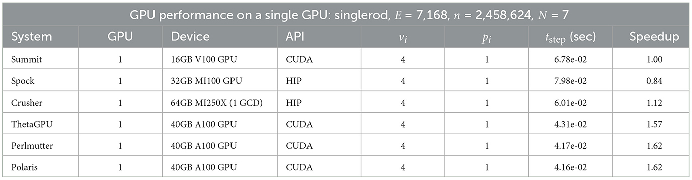
Table 2. NekRS performance on various architectures using a single GPU.

The single-device results of Table 2 show that, for the current version of NekRS,⁴ a single GCD of the MI250X on Crusher realizes a 1.12 × gain in Navier–Stokes solution performance over a single V100 on Summit. Similarly, the A100s are realizing ≈ 1.6-fold gain over the V100.

We explore the single-GPU performance as a function of local problem size, n/P (P = 1) in Figure 2 both with (right) and without (left) the characteristics-based timestepping (Equations 2, 3). Various problem sizes are realized for the single-rod geometry by extruding a baseline two-dimensional mesh to comprise one or more levels in the axial flow direction. The polynomial order is N = 7 and the number of quadrature points for the dealiased advection operator is N_q = 11 in each direction, in each element. In these cases, there is no MPI overhead and, as can be seen from the match between Polaris and Perlmutter, no significant system noise. The saturated sustained performance on Polaris/Perlmutter is 1.75 TFLOPS when using characteristics and only 1.00 TFLOPS for the less computer-intensive formulation (Equation 1), which requires only three nonlinear evaluations per timestep (one for each velocity component). The relative drop-off on Frontier, 1.15 → 0.75 TFLOPS, is not as steep, perhaps because a single GCD of the MI250X is sustaining only 3 TFLOPS for the advection kernel whereas the A100 is sustaining 5 TFLOPS, in isolation. On the other hand, Summit manifests a drop of 0.99 → 0.57 TFLOPS, which is roughly the same ratio seen for the A100-based platforms.

Figure 2

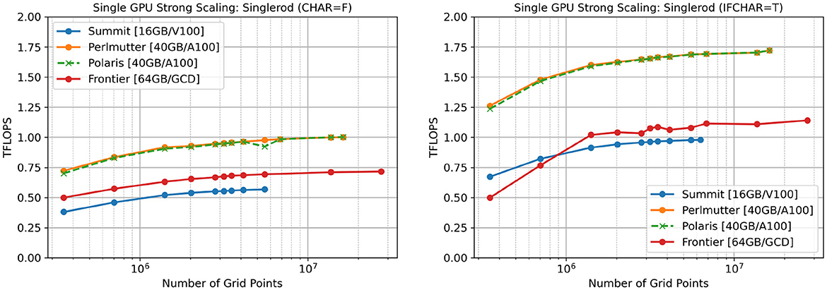
Figure 2. n/P scaling on single-GPU/GCD architectures for single-rod test case: left: using Equation 1 without characteristics timestepping; right: using Equations 2, 3 with characteristics timestepping.

As the problem size diminishes, performance drops from a lack of intra-device parallelism and from the overhead of kernel-launch latency, which becomes important when there is insufficient work to keep the accelerator busy. Consequently, we find n_0.8≈700K for Polaris/Perlmutter for the characteristics-based timestepping (80% efficiency = 1.4 TFLOPS) and n_0.8≈600K without characteristics. For Frontier, n_0.8≈1M with characteristics and ≈900K without. For Summit the corresponding numbers are n_0.8≈1.5M with characteristics and ≈700K without. These n_0.8 values are significantly lower than the n_0.8 = 2M–5M that we observe for production runs described in the next sections, where P≫1, which points to the significance of MPI overhead in the case of multi-GPU simulations.

3 NekRS performance on Frontier vs. Crusher

We next consider multi-GPU performance for ExaSMR's 17 × 17 rod-bundle geometry (Figure 1, right), which we extend in the streamwise direction with 10, 17, and 170 layers, keeping the mesh density the same. This sequence corresponds to 277 thousand spectral elements of order N = 7, for a total of n = 0.27M × 7³ = 95M grid points, 471 thousand spectral elements of order N = 7, for a total of n = 0.47M × 7³ = 161M grid points, and 4.7 million spectral elements of order N = 7, for a total of n = 4.7M × 7³ = 1.6B grid points, respectively. Table 3 summarizes the configurations for these tests.

Table 3

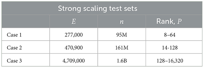
Table 3. Problem setup for strong-/weak-scaling studies.

Simulations are performed for 2,000 steps; and the average time-per-step, t_step, is measured in seconds for the last 1,000 steps. Timestepping is based on Equation 1 with third-order backward-differencing (BDF3) for the time derivative and third-order extrapolation (EXT3) for the nonlinear advection term. The timestep size is Δt = 3.0e-04, which corresponds to a Courant number of CFL = 0.82. We run a single MPI rank per GCD, and there are 8 GCDs per node. On Frontier, rocm/5.1.0 and cray-mpich/8.1.17 were used. On Crusher, simulations were performed with several versions such as rocm/5.1.0, rocm/5.2.0, cray-mpich/8.1.16, and cray-mpich/8.1.19. On Crusher, rocm/5.1.0 is 2%–5% faster than rocm/5.2.0.

Figure 3 shows strong scaling performance of Frontier and Crusher for the three test cases. The left panel shows the average time per step vs. the number of MPI ranks, P. The plot illustrates classic strong scaling as P is increased for fixed problem sizes of n = 95M, 161M, and 1.6B on Crusher (black) and on Frontier (red). Dashed lines in sky-blue represent ideal strong-scale profiles for each case. As is typical, larger problem sizes, n, correspond to cases that are able to effectively use a greater number of MPI ranks, P.

Figure 3

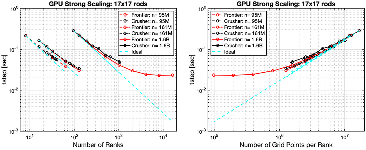
Figure 3. Strong scaling on Frontier and Crusher for 17 × 17 rod bundles with 10, 17, and 170 layers with total number of grid points of n= 95M, 161M, and 1.6B. Average time per step vs. rank, P (left), and average time per step vs. n/P (right). Frontier is set with (cray-mpich/8.1.17, rocm/5.1.0) and Crusher with (cray-mpich/8.1.19, rocm/5.2.0).

The critical observation is that these plots collapse to (nearly) a single curve when the independent variable is number of points per rank, n/P, which is evident in Figure 3, right. This figure illustrates that the strong-scale performance is primarily a function of (n/P) and only weakly dependent on n or P individually, which is in accord with the extensive studies presented in Fischer et al. (2020) and analysis in Fischer et al. (2015). Based on this metric, we can estimate values of (n/P) for a given parallel efficiency and, from there, determine the number of MPI ranks required for a problem of size n to meet that expected efficiency. For example, an efficiency of η_P = 0.80 is realized in this case for n/P≈2M–3M. In the sequel, we explore performance behavior for a variety of problem sizes and platforms, including non-standard “large P” cases where one must consider both n/P and P to forecast performance.

4 NekRS performance on Summit, ThetaGPU, Perlmutter, Polaris, Crusher, and Frontier

In this section, we extend the scaling studies on the 17 × 17 rod bundle simulations to the NVIDIA-based GPU platforms, Summit (V100), ThetaGPU (A100), Perlmutter (A100), and Polaris (A100), and compare these with the AMD MI-250X platforms, Frontier and Crusher. We discuss the performance in detail in Figures 4–6. In Figure 5 we include performance on ThetaGPU. We run one MPI rank per V100 or A100 on the NVIDIA-based nodes and one MPI rank per GCD on the AMD MI250X nodes.

Figure 4

Figure 4. (A–H) Strong-scaling on various GPU architectures for 17 × 17 rod bundle with 10 layers.

Figure 5

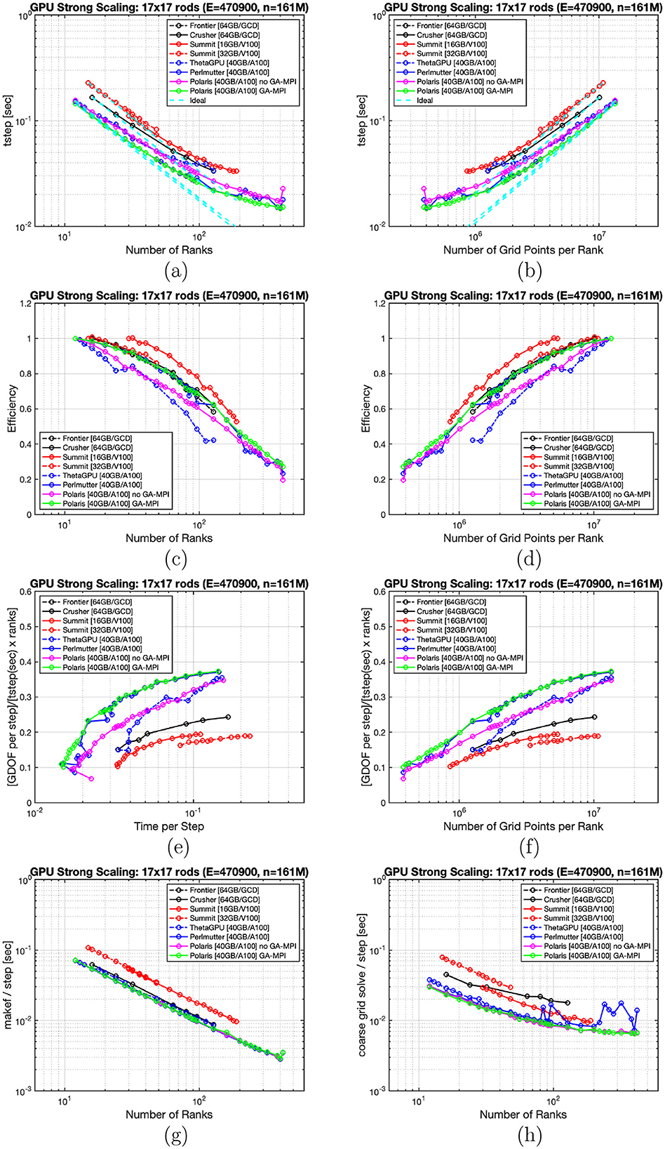
Figure 5. (A–H) Strong-scaling on various GPU architectures for 17 × 17 rod bundle with 17 layers.

Figure 6

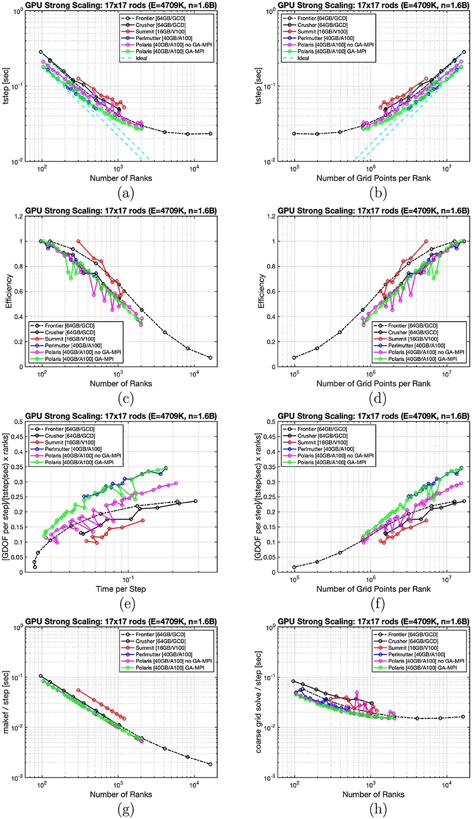
Figure 6. (A–H) Strong-scaling on various GPU architectures for 17 × 17 rod bundle with 170 layers.

Figures 4–6 show t_step as a function of P in (a) and as a function of n/P in (b). Parallel efficiency as a function of P and of n/P is plotted in (c) and (d), respectively. Throughput, in terms of (GDOFS per step)/(time-per-step × P) is plotted versus time-per-step in (e) and vs. n/P in (f). The average time per step for the compute-intensive makef routine, which sets up the dealiased right-hand side of Equation 1, is plotted in (g), and the average time per step for the communication-intensive coarse-grid solve is plotted in (h).

We point out that these strong-scaling plots start from a high level of performance. NekRS currently leverages extensive tuning of several key FP64 and FP32 kernels in libParanumal, including the standard spectral element Laplacian matrix-vector product, local tensor-product solves using fast diagonalization, and dealiased evaluation of the advection operator on a finer set of quadrature points. These kernels are sustaining 3–5 TFLOPS FP64 and 5–8 TFLOPS FP32, per GPU or GCD. At the strong-scale limit, with MPI overhead, NekRS is sustaining ≈ 1 TFLOPS per rank (i.e., per A100 or GCD) for the full Navier–Stokes solution (Merzari et al., 2023). We also note that NekRS selects either host-based MPI or GPU-aware MPI for each kernel communication handle by making runtime tests to determine which option is fastest. We will refer to the GPU-aware MPI cases as GA-MPI in the legends and text.

From Figure 4D, one can readily identify the key scalability metric, n_0.8, as the value of the n/P where the efficiency is 0.8 for the case n = 95M. Here we find n_0.8 < 2M for Summit and GA-Polaris, n_0.8 = 2M for Frontier, and n_0.8 = 4M for Polaris without GA-MPI. We remark that the value of n_0.8 is smaller for the relatively small values of n and P in Figure 4 than it is for the larger (n, P) pairs of Figures 5, 6. One reason is that the coarse-grid costs rise relatively quickly when the processor count is low. Another is that the nearest-neighbor communication required for operator evaluation does not begin to saturate until P>26. Below this value, the domain partitioner will invariably assign each processor to a subdomain that is connected to the boundary. Once the problem is larger, more MPI ranks will have subdomains that are completely within the domain interior and will therefore have more communication. If the domain and decomposition were perfect tensor products, the smallest number of subdomains where communication saturates would be for P = 27. Even then, only one domain would be in the interior and it would generally not need to wait on neighboring subdomains to make their surface data available, as they would be underworked.

Figure 4E indicates that a remarkably small t_step value of 0.025 second is realizable on Polaris, albeit at 60% efficiency. Figure 4G shows that the time in the advection update strong-scales quite well, as would be expected. The curves for the single GCD and A100 collapse to nearly the same performance while the older V100 technology of Summit is about 1.5 × slower. In the absence of communication, this kernel is sustaining 3–4 TFLOPS FP64 on these newer architectures, although the graphs here do include the communication overhead. By contrast, Figure 4H shows the performance for the communication-intensive coarse-grid solve, which is performed using Hypre on the host CPUs. Here, Crusher, Frontier, and Summit show relatively poor performance compared to Polaris and Perlmutter, although the performance also falls off for the latter once P>20, which corresponds to a local coarse-grid problem size of ≈E/P = 277,000/20=13,850 unknowns per rank. Note that the coarse solve is completely executed on the hosts, so there is no performance difference with or without GPU-aware MPI.

As we increase the problem size to n = 161M (Figure 5), the Polaris-GA efficiency curve coalesces with Perlmutter. We find n_0.8 = 2M for Summit and n_0.8≈2.8M for Frontier, Crusher, Perlmutter, and Polaris-GA. ThetaGPU and Polaris without GA have n_0.8 = 4.5M, which means that one can only use half the number of processors in these cases if one is targeting 80% efficiency in production runs, which in turn implies a two-fold increase in time-to-solution. In Figure 5G we see that Summit is ≈1.5 × slower in evaluating the nonlinear term (makef) than the other platforms and that, along with Crusher, it is slower for the host-based coarse-grid solves (h). At larger processor counts, Perlmutter also exhibits noise in the coarse-grid solve, as evidenced by the large oscillations in the strong-scale plot, (h).

Moving to the largest case of n = 1.6B, shown in Figure 6, we see that Polaris exhibits system noise both with and without GA-MPI, as is clear from the parallel efficiency plots (c) and (d). From (h), we can see that the noise is due to the communication-intensive coarse-grid solve, which is susceptible to network congestion. Looking at efficiency vs. n/P (d), Frontier and Summit exhibit n_0.8≈2.8M–3M, while the other platforms are clustered around n_0.8 = 5M. If one is willing to accept ≈ 38% efficiency, per-step times as low as 0.025 s can be realized on Polaris.

The most crucial observation from Figure 6, is that production runs at 80% efficiency will have roughly the time-to-solution on Frontier as on Polaris, despite the relatively high throughput (GDOFS) of Polaris that is evident in row 3, left. At n_0.8 = 3M, Frontier has t_step = 0.065 s. For Polaris, at n_0.8≈4.7M, t_step≈0.066 s. The performance advantage of the A100 is offset by the increased n_0.8 and both platforms exhibit the same time-to-solution. There is of course enough variance in these results, especially with respect to problem size, that either machine could end up with a demonstrable advantage under slightly different circumstances. The key point here, however, is to understand how large the problems are, per rank, under production circumstances and to build and optimize algorithms accordingly.

5 Discussion

In this section we discuss a variety of “anomalous” behaviors encountered in these studies. By anomalous we mean adverse behaviors that either appear or disappear with software and hardware updates. One could argue that these are passing phenomena not worthy of reporting. However, as users work on these platforms it is important to understand potential pitfalls in system performance that might directly impact their own timing studies or production runtimes.

The behaviors described here include the performance of the large-memory (32 GB vs. 16 GB) nodes on Summit, the use of a nonmultiple of 8 ranks on Crusher, the influence of GPU-direct communication on Polaris, the upgrade from Slingshot 10 to Slingshot 11 on Perlmutter, and network interactions with GPU-aware MPI for large node counts on Frontier.

5.1 Performance on Summit V100 16 GB vs. 32 GB

Most of the 4608 nodes on Summit have 16 GB of device memory, which limits how small one can take P₀ in the efficiency definition (Equation 7). A few nodes, however, have 32 GB, which allow one to fit more points onto each V100. Unfortunately, as seen in Figure 5, the Summit 32 GB curves perform about 10% slower than their 16 GB counterparts. The last row of graphs in Figure 5 is particularly revealing—one can see from the makef plot that the V100s perform at the same rate for both the 16 GB and 32 GB nodes but that the host-based coarse-grid solve costs differ by almost 1.5 ×, which indicates either an excessive device-host communication overhead or some type of interhost communication slowdown for the 32 GB nodes.

5.2 Performance on Crusher with rank dependency

In our timing studies we typically do not require that each node be fully occupied. This happens, for example, if one wants to make a device-to-device comparison between Summit, with six V100 per node, and Crusher, which has 8 GCDs per node. Our initial plot of Crusher timing data (not shown) appeared to be very erratic in its dependence on P. Closer inspection, however, revealed that the performance for mod(P, 8) ≠ 0 was about 2 × slower than for the case of mod(P, 8) = 0. Unlike the Summit behavior of the preceding section, this was clearly a device issue and not a host issue. Performance of the makef routine that implements Equation 1 was 2 × slower if mod(P, 8) ≠ 0, but the host-based coarse-grid solve was the same for all values of mod(P, 8). This anomaly was ultimately resolved and did not appear as an issue on Frontier.

5.3 Performance on Polaris with GPU-aware MPI

As expected, communication overhead is more significant without GA-MPI, and consequently the no GA-MPI curves on Polaris show relatively poor performance as the amount of local work, n/P, is reduced. For example, in row 2, right, of Figure 5 the n_0.8 for Polaris with GA-MPI is 2.5M, whereas it is 4.5M without GA-MPI. In the last row of the same figure we see that neither makef nor the coarse-grid solve are influenced by the presence or absence of GA-MPI. For makef, communication does not matter. The coarse-grid solve is communication intensive, but all of that communication originates from the host. We can also see in the results of Figure 6 that the no GA-MPI results are relatively noisy.

5.4 Performance on Perlmutter with Slingshot 10 vs. Slingshot 11

One other discovery was a sudden change in the behavior of Perlmutter at NERSC. Polaris and Perlmutter have similar architectures, so it was expected that they would have similar performance, as is indeed evident in, for example, Figure 7. Later in our studies, however, the Perlmutter interconnect was upgraded from Slingshot 10 (SS10) to Slingshot 11 (SS11). The performance started to vary radically with P, albeit in a highly repeatable fashion, which indicated that the issue was not network noise.

Figure 7

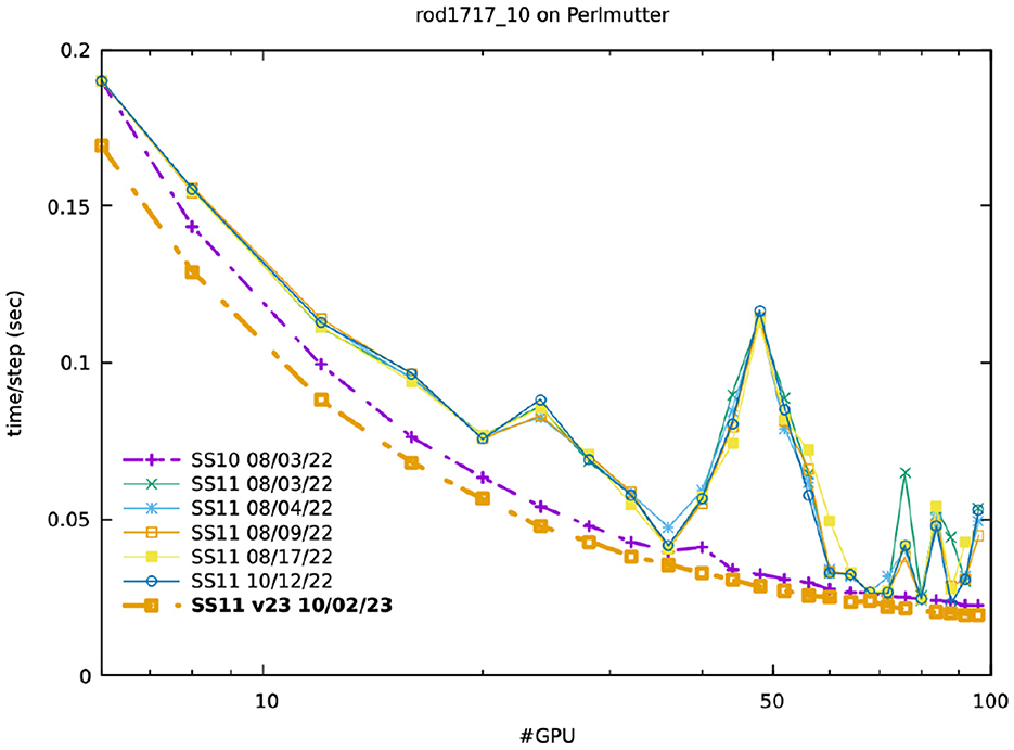
Figure 7. Strong-scaling on Perlmutter with runs using SS10 and SS11 on different days for 17 × 17 rod bundle simulations with 10 layers.

The strong-scaling plot in Figure 7 illustrates the problem for the n = 95M 17 × 17 rod-bundle case of Figure 4. For P = 48 ranks, the Navier–Stokes runtime with SS11 jumps by a factor of 3 over that with SS10. These were repeatable results, as evidenced by timings over a period of several months. Our timing profiles indicated that the anomaly was neither a GPU issue, since makef timings were essentially identical for SS10 and SS11, nor a host-to-host communication issue, since the coarse-grid times were also nearly the same. Inspection of the NekRS profiles showed that the SS11 timing increase was focused in the non-local Schwarz-based smoother for the p-multigrid preconditioner of the pressure Poisson problem, which was running 10 × slower than its SS10 counterpart. Below, we show the profiles for the two simulations with P = 48 (which was the slowest case). Remarkably, the issue was found to be related to short messages, since it arose only at the coarsest levels for the GPU-based communication of the p-multigrid solver, which was employing 32-bit reals.

Fortunately, a later release of SS11 restored the expected performance of the SS11 network, with minimal variance over a wide range of processor counts, as seen by the gold dashed-dot line in Figure 7. For P = 6, the 1.5 × gain in the SS11 bandwidth is manifest as an 11% Navier-Stokes performance gain over SS10. For larger values of P, SS11 continues to offer performance benefits over SS10, but the gains are somewhat diminshed because the messages are smaller and hence tend to be latency-bound rather than bandwidth bound.

SS10 profile:

   name                    time             %  calls

    setup                 3.82904e+01s  0.38  1

      loadKernels         1.03634e+01s  0.27  1

    udfExecuteStep        4.79398e-03s  0.00  2001

    elapsedStepSum        6.13724e+01s  0.62

    solve                 6.12031e+01s  0.61

      min                 2.31879e-02s

      max                 5.51687e-02s

      flop/s              3.36729e+13

  

      makef               5.59237e+00s  0.09  2000

        udfUEqnSource     3.98969e-02s  0.01  2000

      udfProperties       4.82886e-03s  0.00  2001

      velocitySolve       1.73346e+01s  0.28  2000

        rhs               2.29362e+00s  0.13  2000

      pressureSolve       3.42052e+01s  0.56  2000

        rhs               4.69203e+00s  0.14  2000

        preconditioner    2.26178e+01s  0.66  2470

          pMG smoother    1.51609e+01s  0.67  9880

          coarse grid     5.33568e+00s  0.24  2470

        initial guess     3.18958e+00s  0.09  2000

 

SS11 profile:

   name                    time             %  calls

    setup                 3.98696e+01s  0.16  1

      loadKernels         8.86541e+00s  0.22  1

    udfExecuteStep        4.79946e-03s  0.00  2001

    elapsedStepSum        2.06042e+02s  0.84

    solve                 2.05867e+02s  0.84

      min                 5.50540e-02s

      max                 3.32500e-01s

      flop/s              1.00108e+13

  

      makef               5.57575e+00s  0.03  2000

        udfUEqnSource     3.99624e-02s  0.01  2000

      udfProperties       4.88246e-03s  0.00  2001

      velocitySolve       1.72489e+01s  0.08  2000

        rhs               2.29522e+00s  0.13  2000

      pressureSolve       1.79243e+02s  0.87  2000

        rhs               4.48683e+00s  0.03  2000

        preconditioner    1.67813e+02s  0.94  2470

          pMG smoother    1.49445e+02s  0.89  9880

          coarse grid     5.53950e+00s  0.03  2470

        initial guess     3.20173e+00s  0.02  2000

For completeness, we also include the kernel performance numbers as reported in the NekRS logfiles:

SS10 profile:

    Ax: N=7 FP64 GDOF/s=13.2 GB/s=1260 GFLOPS=2184 kv0

   Ax: N=7 FP64 GDOF/s=13.2 GB/s=1260 GFLOPS=2183 kv0

   Ax: N=3 FP64 GDOF/s=12.6 GB/s=1913 GFLOPS=1883 kv5

  

   Ax: N=7 FP32 GDOF/s=25.0 GB/s=1194 GFLOPS=4145 kv4

   Ax: N=3 FP32 GDOF/s=18.0 GB/s=1368 GFLOPS=2693 kv2

  

  fdm: N=9 FP32 GDOF/s=44.9 GB/s= 812 GFLOPS=7452 kv4

  fdm: N=5 FP32 GDOF/s=34.1 GB/s= 825 GFLOPS=4301 kv1

  

  flop/s  3.36729e+13  (701 GFLOPS/rank)

 

SS11 profile:

    Ax: N=7 FP64 GDOF/s=13.2 GB/s=1256 GFLOPS=2179 kv0

   Ax: N=7 FP64 GDOF/s=13.2 GB/s=1257 GFLOPS=2180 kv0

   Ax: N=3 FP64 GDOF/s=12.6 GB/s=1912 GFLOPS=1882 kv5

  

   Ax: N=7 FP32 GDOF/s=25.0 GB/s=1194 GFLOPS=4144 kv5

   Ax: N=3 FP32 GDOF/s=18.1 GB/s=1369 GFLOPS=2696 kv2

  

  fdm: N=9 FP32 GDOF/s=44.9 GB/s= 812 GFLOPS=7444 kv4

  fdm: N=5 FP32 GDOF/s=34.1 GB/s= 825 GFLOPS=4303 kv1

  

  flop/s  1.00108e+13  (208 GFLOPS/rank)

In SS10 profile and SS11 profile, kv reflects the particular kernel version chosen out of the suite of available kernels in NekRS for the particular operation. We see that the 64-bit Ax kernels (the matrix-vector product with the Laplace operator for spectral element order N) realize ≈2 TFLOPS per device, while their 32-bit counterparts realize 3–4 TFLOPS (32-bit arithmetic is used in the preconditioner only). The fdm kernel implements the fast-diagonalization method described earlier for the overlapping Schwarz preconditioners. This is a fast operation and can be seen to sustain > 7 GFLOPS (FP32). Note that, as expected, the kernel performance, which does not include any MPI overhead, is not dependent on the Slingshot version. NekRS also reports the total observed GFLOPS, which is seen to be 701 GFLOPS/rank for SS10 and 208 GFLOPS/rank for SS11 with P = 48, prior to the bug fix.

5.5 Network issues for large-P runs on Frontier

Our largest runs to date have been on 72,000 MPI ranks of Frontier (Merzari et al., 2023). Unfortunately, above several thousand nodes, the Frontier network exhibited erratic behavior such that the sustained performance for the default version of NekRS dropped to ≈150 GFLOPS/rank. The performance is illustrated in Figure 8 (left), which shows the NekRS time-per-step on 9000 nodes (P = 72000) for a simulation with 500 layers of the full-core geometry of Figure 1 (left). The fluid domain had n = 172B gridpoints while the solid domain (for conduction in the individual rods) had n_s = 198B gridpoints. In Figure 8 (left), we see that a lower bound time-per-step of t_step≈0.3s, which is the performance level we would expect, and a cloud of points above that with t_step as high as 10s, which is >30 × the expected value. Testing for these full-scale runs was challenging because of system stability issues. The limited tests that were feasible, however, indicated that the significant variance arose from from flooding the system network during the relatively simple (and normally fast) Jacobi-preconditioned Helmholtz solves Equation 5 for velocity. Tests indicated that the flooding could be mitigated by moving from block (uvw) solves in the velocity to scalar (u, v, w) solves for each component (i.e., smaller messages instead of fewer large messages). It was found however, that among the limited trials that time permitted, turning off GPU-direct and routing the messages through the host was the better option, with results illustrated Figure 8 (right) for an 800-layer case that sustains 390 GFLOPS per rank for P = 72000.

Figure 8

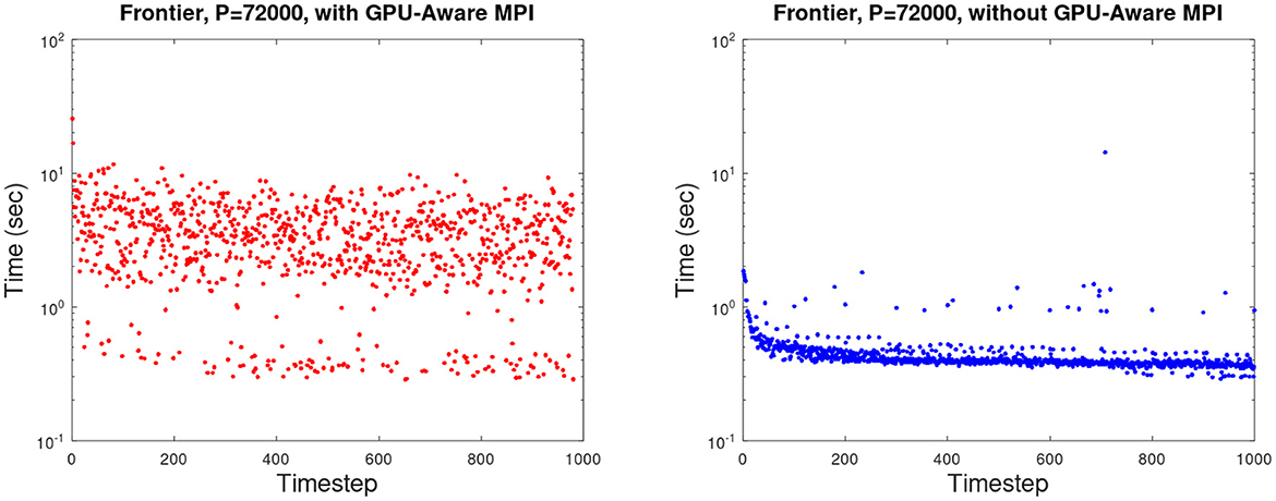
Figure 8. Navier-Stokes time-per-step for P = 72, 000 runs on Frontier: (left) 500-layer full-core configuration of Figure 1 with GPU-aware MPI; (right) 800-layer case without GPU-aware MPI.

6 Conclusions

We explored the performance of a highly-tuned incompressible flow code, NekRS, on current-generation HPC architectures featuring accelerator-based nodes. The principal accelerators under consideration are the NVIDIA V100, NVIDIA A100, and MI250X with eight GCDs per node. We found that the raw performance of a single GCD is about 85% of a single A100. We also found that the AMD-based Crusher platform had slower host-based communication than its Polaris/Perlmutter counterpart, as witnessed by the relatively poor performance of the Hypre-based coarse-grid solver, which runs on the host. This situation is significantly improved on Frontier.

We further identified that, despite having lower throughput, Frontier had better scalability (i.e., lower n_0.8) than the NVIDIA A100 platforms Perlmutter and Polaris, which led to Frontier having a slight advantage in time-to-solution (although the advantage was arguably within the variance arising from system noise).

A key finding was that n_0.8 = 2M–5M are typical values of n/P required to sustain 80% parallel efficiency on DOE's current set of leadership HPC platforms. This number is of interest for algorithmic (and hardware?) optimization because this will be the most likely operating point for production users. Running with n/P≫n_0.8 will result in significant slow-down. Running with n/P≪n_0.8 will result in significant waste of an allocation. Moreover, under these production-run conditions, time-to-solution (here, t_step) depends strongly on n/P and only weakly on n or P individually. As a consequence, one can predict t_step with reasonable fidelity for any problem size n provided it does not saturate the full machine (meaning n/P<n_0.8, where P is the maximum number of processes available).

Finally, several examples of anomalous behavior that were encountered during the study were identified and discussed, and ultimately resolved either by system upgrades or by altering execution paths to avoid the source of difficulty.

Data availability statement

Publicly available datasets were analyzed in this study. This data can be found here: https://github.com/Nek5000/nekRS.

Author contributions

MM: Conceptualization, Data curation, Formal analysis, Funding acquisition, Investigation, Methodology, Project administration, Resources, Software, Supervision, Validation, Visualization, Writing – original draft, Writing – review & editing. Y-HL: Data curation, Investigation, Methodology, Software, Validation, Visualization, Writing – review & editing. PF: Conceptualization, Formal analysis, Funding acquisition, Investigation, Methodology, Project administration, Resources, Software, Supervision, Validation, Writing – original draft, Writing – review & editing. TR: Investigation, Software, Validation, Writing – review & editing. JH: Data curation, Investigation, Resources, Software, Writing – review & editing.

Funding

The author(s) declare financial support was received for the research, authorship, and/or publication of this article. This material was based upon work supported by the U.S. Department of Energy, Office of Science, under contract DE-AC02-06CH11357 and by the Exascale Computing Project (17-SC-20-SC). The Oak Ridge Leadership Computing Facility at the Oak Ridge National Laboratory was supported by the Office of Science of the U.S. DOE under Contract No. DE-AC05-00OR22725. The Argonne Leadership Computing Facility at Argonne National Laboratory was supported by the Office of Science of the U.S. DOE under Contract No. DE-AC02-06CH11357.

Acknowledgments

This research used resources at the Argonne and the Oak Ridge Leadership Computing Facility. This research also used resources of the National Energy Research Scientific Computing Center, a DOE Office of Science User Facility using NERSC award ALCC-ERCAP0030677.

Conflict of interest

The authors declare that the research was conducted in the absence of any commercial or financial relationships that could be construed as a potential conflict of interest.

Publisher's note

All claims expressed in this article are solely those of the authors and do not necessarily represent those of their affiliated organizations, or those of the publisher, the editors and the reviewers. Any product that may be evaluated in this article, or claim that may be made by its manufacturer, is not guaranteed or endorsed by the publisher.

Footnotes

1. ^We prefer dofs per second per rank because AMD's MI250X has two compute units (GCDs) per GPU and Aurora's Intel has two tiles per PVC—users view these as two processors

2. ^We typically take the average time over several hundreds or thousands timesteps.

3. ^For fluid flow simulations, some authors set n to be 4 times the number of grid points because there are typically three velocity components and one pressure unknown at each grid point. We prefer to take n to be the number of grid points. The problems are generally large enough that we do not need to distinguish between interior points where the solution is unknown and surface points where boundary data is prescribed. We simply set n to represent the union of these sets given that some quantities might have Neumann conditions on the boundary while others have Dirichlet.

4. ^NekRS version 22.0 is used.

References

Abdelfattah, A., Barra, V., Beams, N., Bleile, R., Brown, J., Camier, J.-S., et al. (2021). GPU algorithms for efficient exascale discretizations. Par. Comput. 108:102841. doi: 10.1016/j.parco.2021.102841

Crossref Full Text | Google Scholar

Anderson, R., Andrej, J., Barker, A., Bramwell, J., Camier, J.-S., Dobrev, J. C. V., et al. (2020). MFEM: A modular finite element library. Comp. Mathemat. Appl. 81, 42–74. doi: 10.1016/j.camwa.2020.06.009

Crossref Full Text | Google Scholar

Arndt, D., Bangerth, W., Davydov, D., Heister, T., Heltai, L., Kronbichler, M., et al. (2017). The deal.II library, version 8.5. J. Num. Math. 25, 137–145. doi: 10.1515/jnma-2017-0058

Crossref Full Text | Google Scholar

Bienz, A., OLson, L., Gropp, W. D., and Lockhart, S. (2021). “Modeling data movement performance on heterogeneous architectures,” in IEEE High Performance Extreme Computing Conference (HPEC) (Waltham, MA: IEEE), 1–7.

Google Scholar

Chalmers, N., Karakus, A., Austin, A. P., Swirydowicz, K., and Warburton, T. (2020). libParanumal: A Performance Portable High-Order Finite Element Library. doi: 10.5281/zenodo.4004744

Crossref Full Text | Google Scholar

Chalmers, N., Mishra, A., McDougall, D., and Warburton, T. (2023). HipBone: a performance-portable graphics processing unit-accelerated C++ version of the NekBone benchmark. Int. J. High Perf. Comput. Appl. 37, 560–577. doi: 10.1177/10943420231178552

Crossref Full Text | Google Scholar

Deville, M., Fischer, P., and Mund, E. (2002). High-Order Methods for Incompressible Fluid Flow. Cambridge: Cambridge University Press.

Google Scholar

Fischer, P., Heisey, K., and Min, M. (2015). “Scaling limits for PDE-based simulation (invited),” in 22nd AIAA Computational Fluid Dynamics Conference, AIAA Aviation (Dallas, TX).

Google Scholar

Fischer, P., Kerkemeier, S., Min, M., Lan, Y., Phillips, M., Rathnayake, T., et al. (2021). NekRS, a GPU-accelerated spectral element Navier-Stokes solver. arXiv [preprint] arXiv:2104.05829. doi: 10.48550/arXiv.2104.05829

Crossref Full Text | Google Scholar

Fischer, P., Kerkemeier, S., Min, M., Lan, Y.-H., Phillips, M., Rathnayake, T., et al. (2022). NekRS, a GPU-accelerated spectral element Navier–Stokes solver. Par. Comput. 114:102982. doi: 10.1016/j.parco.2022.102982

Crossref Full Text | Google Scholar

Fischer, P., Lottes, J., and Kerkemeier, S. (2008). Nek5000: Open source spectral element CFD solver. Available at: http://nek5000.mcs.anl.gov; https://github.com/nek5000/nek5000

Google Scholar

Fischer, P., Min, M., Rathnayake, T., Dutta, S., Kolev, T., Dobrev, V., et al. (2020). Scalability of high-performance PDE solvers. Int. J. of High Perf. Comp. Appl. 34, 562–586. doi: 10.1177/1094342020915762

Crossref Full Text | Google Scholar

Kolev, T., Fischer, P., Min, M., Dongarra, J., Brown, J., Dobrev, V., et al. (2021). Efficient exascale discretizations. Int. J. of High Perf. Comp. Appl. 35, 527–552. doi: 10.1177/1094342021102080

Crossref Full Text | Google Scholar

Kronbichler, M., and Ljungkvist, K. (2019). Multigrid for matrix-free high-order finite element computations on graphics processors. ACM Trans. on Par. Comp. 6, 1–32. doi: 10.1145/3322813

Crossref Full Text | Google Scholar

Kronbichler, M., Sashko, D., and Munch, P. (2023). Enhancing data locality of the conjugate gradient method for high-order matrix-free finite-element implementations. Int. J. High Perf. Comput. Appl. 37, 61–81. doi: 10.1177/10943420221107880

Crossref Full Text | Google Scholar

Maday, Y., Patera, A., and Rønquist, E. (1990). An operator-integration-factor splitting method for time-dependent problems: application to incompressible fluid flow. J. Sci. Comput. 5, 263–292. doi: 10.1007/BF01063118

Crossref Full Text | Google Scholar

Malm, J., Schlatter, P., Fischer, P., and Henningson, D. (2013). Stabilization of the spectral-element method in convection dominated flows by recovery of skew symmetry. J. Sci. Comp. 57, 254–277. doi: 10.1007/s10915-013-9704-1

Crossref Full Text | Google Scholar

Medina, D. S., St-Cyr, A., and Warburton, T. (2014). OCCA: A unified approach to multi-threading languages. arXiv [preprint] arXiv:1403.0968. doi: 10.48550/arXiv.1403.0968

Crossref Full Text | Google Scholar

Merzari, E., Hamilton, S., Evans, T., Romano, P., Fischer, P., Min, M., et al. (2023). “Exascale multiphysics nuclear reactor simulations for advanced designs (Gordon Bell Prize Finalist paper),” in Proc. of SC23: Int. Conf. for High Performance Computing, Networking, Storage and Analysis (downtown Denver: IEEE).

Google Scholar

Min, M., Lan, Y., Fischer, P., Merzari, E., Kerkemeier, S., Phillips, M., et al. (2022). “Optimization of full-core reactor simulations on Summit,” in Proc. of SC22: Int. Conf. for High Performance Computing, Networking, Storage and Analysis (Dallas, TX: IEEE).

Google Scholar

OCCA (2021). OCCA: Git Repository. Available at: https://github.com/libocca/occa

Google Scholar

Orszag, S. (1980). Spectral methods for problems in complex geometry. J. Comput. Phys. 37:70–92. doi: 10.1016/0021-9991(80)90005-4

Crossref Full Text | Google Scholar

Patel, S., Fischer, P., Min, M., and Tomboulides, A. (2019). A characteristic-based, spectral element method for moving-domain problems. J. Sci. Comp. 79, 564–592. doi: 10.1007/s10915-018-0876-6

Crossref Full Text | Google Scholar

Patera, A. (1984). A spectral element method for fluid dynamics : laminar flow in a channel expansion. J. Comput. Phys. 54, 468–488. doi: 10.1016/0021-9991(84)90128-1

Crossref Full Text | Google Scholar

Pothen, A., Simon, H., and Liou, K. (1990). Partitioning sparse matrices with eigenvectors of graphs. SIAM J. Matrix Anal. Appl. 11, 430–452. doi: 10.1137/0611030

Crossref Full Text | Google Scholar

Sathyanarayana, S., Bernardini, M., Modesti, D., Pirozzolia, S., and Salvadore, F. (2025). High-speed turbulent flows towards the exascale: STREAmS-2 porting and performance. J. Par. Dist. Comput. 196:104993. doi: 10.1016/j.jpdc.2024.104993

Crossref Full Text | Google Scholar

Vargas, A., Stitt, T., Weiss, K., Tomov, V., Camier, J., Kolev, T., et al. (2022). Matrix-free approaches for GPU acceleration of a high-order finite element hydrodynamics application using MFEM, Umpire, and RAJA. Int. J. High Perf. Comput. Appl. 36, 492–509. doi: 10.1177/10943420221100262

Crossref Full Text | Google Scholar