Auto-scaling edge cloud for network slicing

This paper presents a study on resource control for autoscaling virtual radio access networks (RAN slices) in next-generation wireless networks. The dynamic instantiation and termination of on-demand RAN slices require efficient autoscaling of computational resources at the edge. Autoscaling involves vertical scaling (VS) and horizontal scaling (HS) to adapt resource allocation based on demand variations. However, the strict processing time requirements for RAN slices pose challenges when instantiating new containers. To address this issue, we propose removing resource limits from slice configuration and leveraging the decision-making capabilities of a centralized slicing controller. We introduce a resource control agent (RC) that determines resource limits as the number of computing resources packed into containers, aiming to minimize deployment costs while maintaining processing time below a threshold. The RAN slicing workload is modeled using the Low-Density Parity Check (LDPC) decoding algorithm, known for its stochastic demands. We formulate the problem as a variant of the stochastic bin packing problem (SBPP) to satisfy the random variations in radio workload. By employing chance-constrained programming, we approach the SBPP resource control (S-RC) problem. Our numerical evaluation demonstrates that S-RC maintains the processing time requirement with a higher probability compared to configuring RAN slices with predefined limits, although it introduces a 45% overall average cost overhead.

1. Introduction

Mobile edge computing (MEC) is envisioned as a computational backend in the wireless communication service architecture. It deploys containerized radio applications, i.e., radio access network (RAN) slices, to deliver: (i) Ultra-Reliable and Low-Latency Communication (URLLC); (ii) Enhanced Mobile Broadband (eMBB); and (iii) Massive Machine-Type-Communication (mMTC). Unlike other MEC workloads, RAN slicing workloads have strict processing time requirements (Akman et al., 2020).

Successful deployment of RAN slicing at the edge requires auto-scaling MEC computational resources to meet the variations in RAN slicing workloads without violating processing time requirements. Autoscaling the edge cloud includes resource scaling (vertical) and scaling the application profile according to variations in the application demands for resources (horizontal) (Armbrust et al., 2009). While vertical scaling (VS) tailors (i.e., scales up/down) MEC resources for the running slices within their pre-configured resource limits, horizontal scaling (HS) responds to the growing demands for RAN slices by instantiating a new slice (container) when the running container has demands for resources that exceed its pre-configured resource limits. Starting a new container, which consumes 0.5–5 s (Google, 2022), contravenes end-to-end delay requirements for RAN slicing operation, i.e., 0.5–50 ms (3GPP, 2017). Thus, removing resource limits could minimize processing time by avoiding the potential instantiation of the new container. Moreover, recent technical studies (Khun, 2020; Musthafa, 2020; Henderson, 2022) demonstrated that removing resource limits from containers' configurations led to minimizing processing time, which is needed for RAN slicing workload. Nevertheless, removing resource limits from containers' configuration is inapplicable in MEC operation due to limited resources at the edge. Thus, carefully considering resource usage among running slices is necessary to autoscale the edge cloud for RAN slices.

Auto-scaling MEC for RAN slices introduces a critical research question, which is “Can resource limits be soft-tuned according to variation in demands rather than using pre-defined resource limits to auto-scale MEC for RAN slices ?” This paper addresses this question by migrating resource limits from containers' configuration files to a centralized entity that determines them as outcomes of a decision-making process. Fortunately, the RAN slicing architecture defines a slicing controller that orchestrates running slices (Akman et al., 2020), which could embrace an autoscaling framework to dynamically scale up/down resources to match expansion/reduction in radio workload without instantiating a new container. Thus, the autoscaling framework includes a resource control agent (RC) that deploys the decision-making process to tune resource limits according to the variations in slices' workloads. The decision-making process aims to minimize the cost of running slices (i.e., minimize the number of allocated resources per running container) while the processing delay is maintained below a pre-defined threshold. In this regard, we introduce a variant of the bin packing problem (BPP) to determine resource limits by modeling containers, which process radio workload as bins and computational resources as items that need to be packed into bins. The amount of packed items (computational resources) determines the containers' limits.

Developing the decision-making process for the RC design requires modeling RAN slicing workloads to reflect the variations in demands for MEC resources. To facilitate modeling RAN slicing workloads, we consider surveillance (Yuan and Muntean, 2020) and Industry 4.0 (Garcia-Morales et al., 2019) use cases of RAN slicing deployments where captured data are offloaded to the MEC that executes all computational kernels to process the received wireless signals for data analysis and the decision-making process. Although several radio and control functions would be processed at the edge, measurements in Foukas and Radunovic (2021) show that the low-density parity check (LDPC) coding algorithm consumes 60% of uplink execution time and 50% of total (i.e., uplink and downlink) execution time in 5G cloud RAN systems. Therefore, we take a step toward modeling RAN slicing workloads by adopting the asymptotic analysis of the LDPC decoding algorithm (Bae et al., 2019).

Accordingly, we leverage the stationary random distribution of the LDPC's iterations¹ to model the fluctuations in radio workload (i.e., variations in demands). The number of LDPC iterations depends on the quality of the received signals (i.e., a higher-quality received signal reduces the number of LDPC iterations). Based on analysis in Sharon et al. (2006), this paper models the number of iterations as a Gaussian random variable $\tilde{R}$ where a Binary Additive White Gaussian Noise (BiAWGN) channel model is assumed for wireless propagation. Accordingly, a processing delay is developed as a function of LDPC operations and MEC power, defined using the Roofline model (Williams et al., 2009). Hence, we address the problem of packing MEC's processing cores (items) into LDPC containers (bins), which manifests random variations in demands, i.e., Gaussian random number of iterations. Hence, the BPP introduces a stochastic processing time constraint since LDPC operations are defined as a function of $\tilde{R}$.

Chance-constrained stochastic programming (CCSP) is used for the stochastic BPP-based resource control (S-RC) as it demonstrates success for manipulating the SBPP in cloud datacenters (Yan et al., 2022). First, through CCSP, we formulate the S-RC problem with probabilistic processing delay constraint. Then, we transform it into a deterministic formulation using the inverse cumulative distribution function (inverse-CDF) of $\tilde{R}$. Afterward, we linearize it and use the Branch-and-Cut algorithm (Mitchell, 2002) to solve the resulting combinatorial optimization problem.

We evaluate the S-RC performance numerically by introducing a probabilistic metric, defined as the probability of processing time violation, i.e., the probability that processing time τ is more significant than a pre-defined threshold δ. We measure the probability P_τ>δ of legacy RC vs. S-RC. In legacy RC, we assume pre-defined resource limits are set for each container where the RC deploys HS to start a new container. Results show that S-RC maintains processing time τ below threshold δ with lower P_τ>δ than legacy RC for dense and enormous input data size. However, the overall average cost overhead of S-RC deployment (i.e., packing additional computing resources) is 45% higher than RC, particularly with slices with ultra-low processing time requirements (i.e., δ is very small) and enormous input data size.

The subsequent sections explain our methods to solve and evaluate the S-RC and discuss the numerical results in more detail. First, Section 2 explains the system model, problem formulation, and optimization methods we use to approach the S-RC. Following that, we show the numerical evaluations in Section 3. Then, results and recommendations for a robust design of autoscaling framework for RAN slicing are discussed in Section 4. Finally, Section 5 concludes the paper and outlines future work.

2. System design and autoscaling methods

Radio Access Network (RAN) slicing introduces a novel service architecture for network operation where many service providers, i.e., multiple mobile virtual network operators (MVNOs), lease physical resources from a few infrastructure providers (InPs) to provide virtualized wireless communication services. Figure 1 demonstrates a RAN slicing design framework where InPs lease their network and computational resources to various tenants, i.e., mobile virtual network operators (MVNOs). In this context, we consider network resources at the edge, including radio units (RUs), wireless spectrum, and a transport network that connects RUs to the edge cloud at the proximity of wireless infrastructure to provide low-latency computational service for different wireless use-cases. Although end-to-end network slicing architecture encompasses slicing core cloud and data network resources, this paper discusses the resource allocation problem at the edge for surveillance and Industry 4.0 use-cases (Garcia-Morales et al., 2019; Fitzek et al., 2020; Yuan and Muntean, 2020). In particular, we focus on managing computational resources at the edge, a.k.a multi-access (mobile) edge computing (MEC), which manifests the computational infrastructure for wireless slices operation.

FIGURE 1

Figure 1. RAN slicing design. (A) RAN slicing framework. (B) Inside local slicing controller.

RAN slicing architecture introduces global and local slicing control agents. As depicted in Figure 1A, InPs deploy the global slicing controller to maximize their revenue while tenants' service level agreements (SLAs) are satisfied. Therefore, admission control (AC) interplays with the resource manager (RM) to admit (reject) a tenant's (MVNO's) request for RAN slices. In this context, RM tracks the variations in available resources according to tenant resource usage changes (i.e., instantiation/termination of a MVNO's slices would affect resource availability). Furthermore, RM interacts with the slicing scheduler to schedule a MVNOs' slicing workloads among allocated resources for low-latency slice instantiation. On the other hand, each tenant deploys a local slicing controller to manage its leased resources (i.e., allocated resources by the global slicing controller) for its running slices. Figure 1B demonstrates the components of the local slicing controller that would dynamically scale network and computational resources at the edge for the tenant's running RAN slices. Furthermore, it is shown that dynamic scaling of the computational resources would be carried out by adopting the autoscaling framework of Kubernetens-like systems (Google, 2022; Microsoft, 2022), which would manage the containerized backend of RAN slices at the edge computing. In this sense, autoscaling computational resources would interplay with the dynamic scaling of wireless network resources by deploying a coordinator agent. We refer to 3GPP (2018), Yan et al. (2019), D'Oro et al. (2020), and Liu et al. (2020) for an insightful discussion on the design of coordinator, autoscaling network resources, and the global slicing control.

Figure 1B shows the deployment of Kubernetes-like autoscaling algorithms in a centralized entity, i.e., Kubernetes' controller node (master node), which manages MEC resources for running containers (Pods) in worker nodes. The statistics of containers' resource usage are the essence of the autoscaling framework. Based on a user-defined (customized) deployment metric (e.g., CPU throttling, CPU usage, memory usage, out-of-memory statistics, etc.), a recommender agent uses statistical histogram methods to estimate upper and lower bounds of the customized metric according to the collected measurements during the last scaling cycle. An updater agent decides whether horizontal scaling (HS) or vertical scaling (VS) procedures should be invoked according to the recommender's output (estimated deployment metric). HS is invoked if the deployment metric indicates that more resources than predefined limits are needed for a running container. Accordingly, the updater requests the admission controller to instantiate a new container. If required resources are insufficient to instantiate a new container, the admission controller (AC) consults the resource control manager to scale down other running containers whose resource usage is below their predefined resource limits. VS is invoked when the estimated metric indicates that a running container's resource usage is growing but below the pre-defined resource limit (request the AC for scaling up) or declining (request the AC for scaling down). Based on the AC's decision, a scheduler agent makes its scheduling decisions for scaled-up/down containers and any new instantiated container. Therefore, autoscaling MEC resources becomes critical for RAN slicing design to meet the dynamic variations in radio workload at the edge.

Unlike autoscaling cloud resources for delay-tolerant workloads, autoscaling MEC resources should consider the processing time requirement of delay-sensitive radio workloads, i.e., end-to-end delay requirements must be within 0.5–50 ms for different wireless services. While HS instantiates a new container when a container requests more resources than pre-configured resource limits, VS scales up/down resources to a container according to the variations in workload provided that resource requests are below the defined resource limits. Thus, HS adds delay overhead due to the time to start a container, i.e., 0.5–5 s, which violates end-to-end delay requirements for RAN slicing design. Furthermore, performance evaluations in Khun (2020), Musthafa (2020), and Henderson (2022) recommend removing resource limits from container configuration to maintain a low processing delay.

Removing resource limits could be beneficial to satisfy delay requirements for RAN slicing workloads. Furthermore, resource limit removal would lead to HS displacement since HS works when the workload uses more resources than pre-configured limits. However, the need for more computational resources at the edge makes resource limit removal an unattainable solution for RAN slicing design. Thus, a critical research for autoscaling design RAN slicing is “Can resource limits be soft-tuned according to variation in demands rather than using pre-defined resource limits to auto-scale MEC for RAN slices ?” This paper paves the way to answer this question by leveraging the capability of the local slicing controller, which orchestrates the RAN slicing operation, to embrace an autoscaling framework with a resource control agent (RC) to tune resource limits according to the variations in the running slices' workloads. Hence, resource limits would be removed from configuration of RAN slices (containers) but would be determined by the RC as outcomes of a decision-making process.

The following subsections present material for the system model and discuss methods for developing the RC decision-making process to determine resource limits for RAN slicing.

2.1. Material for system design

2.1.1. Assumptions

2.1.1.1. RAN slicing workload

Modeling RAN slicing workloads is challenging since deployments are only emerging. To circumvent this challenge, we consider two use cases of RAN slicing deployment: (i) surveillance; and (ii) Industry 4.0. Both cases consider offloading captured data to the MEC, which processes the received wireless signal by executing all computational kernels for data analysis and decision-making. In wireless surveillance applications, drones, a.k.a unmanned aerial vehicles (UAVs), offload their encoded observations to the MEC for further data analysis and decision-making process regarding surveillance systems. Thus, drones would encode, modulate, and transmit raw observations to the MEC that demodulate and decode received signals. Hence, drones would be supported by eMBB and URLLC containers for real-time video transmission and vehicular communication services, respectively. In Industry 4.0, many sensors transmit encoded measurements to MEC for autonomous production (i.e., MEC would deploy a decision-making process that generates control signals according to received measurements to manage an actuator in the production field). Accordingly, mMTC and URLLC containers would support massive sensor-MEC low-latency data communication and control.

The RAN slicing deployments mentioned above include processing various radio functions, e.g., (de)modulation, channel (de)coding, layer (de)mapping, channel estimation, multi-in-multi-out (MIMO) pre-coding, etc. However, given the lack of technical studies that characterize variations in RAN slicing workload, we consider the most significant radio functions to model fluctuations in radio workload. Measurements in Foukas and Radunovic (2021) demonstrate that the channel decoding task, which deploys the Low-Density Parity Check (LDPC) decoding algorithm (Bae et al., 2019), is the most expensive computational task. It contributes 60% of execution time to the uplink processing time and 50% of execution time to the total downlink and uplink processing time. Therefore, to introduce a case study of modeling the RAN slicing workload, we adopt LDPC to model the radio workload.

LDPC is an Iterative-based Belief Propagation algorithm, i.e., Message Passing Algorithm (MPA), used for error detection and correction of the received message transmitted over a noisy channel (Maguolo and Mior, 2008; Chandrasetty and Aziz, 2018b). MPA behaves as an iterative sum-product algorithm (SPA) where, in each iteration, there are two basic operations: (i) variable node sum operations (Sum) that perform summation of log-likelihood ratios (LLR) of n-bits that represent the reliability of a decoded message; and (ii) check nodes multiplication operations (product) that estimate the multiplications of LLRs for each bit value (i.e., each check node value). The MPA's iterations depend on the quality of the received signals (Sharon et al., 2006; Maguolo and Mior, 2008). Therefore, we model the MPA's number of iterations as a random variable $\tilde{R}$ that reflects the reliability of a received message (Sharon et al., 2006; Maguolo and Mior, 2008; Chandrasetty and Aziz, 2018b). By following the analysis in Sharon et al. (2006), we define the random distribution of the $\tilde{R}$ as Gaussian distribution where a Binary Additive White Gaussian Noise (BiAWGN) channel model is assumed for wireless propagation.

2.1.1.2. Scaling period

Auto-scaling decision-making occurs at each scaling period, i.e., constant duration scaling cycle (Google, 2022). Nevertheless, we address the auto-scaling problem during a single scaling cycle and skip the iterative property of the problem since we study only one radio function to model the radio workload and assume that the variations in LDPC workload follow the same distribution at each cycle.

2.1.1.3. Computational resources

Since we focus on the processing time design constraint, this paper considers only the processing units to model the computational resources, i.e., only CPUs and GPUs. Studying the impact of memory management on execution time is out of this paper's scope.

2.1.2. System model

2.1.2.1. LDPC

In LDPC (Chandrasetty and Aziz, 2018a), the received message (encoded message) has length n bits that convey a k-bit source message where k<n and $\frac{k}{n}$ is the LDPC code rate. Further, h redundant bits (i.e., parity bits) are added to the source message, where (k = n−h). LDPC codes are generated by constructing a sparse (H) matrix (h rows x n columns); following that, a generator matrix (G) is defined for LDPC code generation. The parity-check sparse matrix H is used at the receiver for error detection and correction. The density of 1's in the H sparse matrix is low; therefore, LDPC is called a low-density Parity Check. A Tanner graph represents the H matrix where h check nodes are connected to n variable nodes through many edges representing the number of non-zero elements in the H matrix.

2.1.2.2. LDPC processing time

To model the processing time of the LDPC decoding algorithm, we adopt two first-order approximation methods: (i) the Roofline analytical model (Williams et al., 2009); and (ii) LDPC algorithmic analysis (Maguolo and Mior, 2008; Chandrasetty and Aziz, 2018b; Hamidi-Sepehr et al., 2018). Roofline introduces a first-order approximation of a function that defines an architecture's peak performance as a function of an application's operational intensity (arithmetic intensity) A. The architecture's peak performance is characterized by its memory bandwidth β (bytes/seconds) and its processing throughput π (operations/seconds) when processing a computational kernel with operational intensity A. A is the ratio of the number of operations to the number of memory reads and writes, which depends on the input data size. We model the MPA's number of operations (MUL + ADD) operations by following the analysis of the MPA's time complexity in Maguolo and Mior (2008) and Chandrasetty and Aziz (2018b). Likewise, we model the MPA's number of memory reads and writes through the MPA's space complexity (Chandrasetty and Aziz, 2018b; Hamidi-Sepehr et al., 2018). In each iteration, there are approximately (2hρ′+4nγ′) multiplications and n additions where ρ′ and γ′ are the average number of ones in the H's rows and H's columns, respectively. Therefore, the number of operations is $\widetilde{OP{S}_{LDPC}}=\tilde{R}.\left[2h{\rho }^{{}^{\prime }}+4n{\gamma }^{{}^{\prime }}+n\right]=\tilde{R}.OP{S}^d$, where OPS^d = [2hρ′+4nγ′+n]. MPA's space complexity is defined as H's size, i.e., hn. Accordingly, $A\approx \frac{\tilde{R}.OP{S}^d}{hnz}$ (Operations/Byte) where z is the variable data size (i.e., 4 Bytes for integer variables). Moreover, the Roofline model defines the peak performance of an architecture that processes a certain computational kernel as min(π, βA). LDPC has a multi-threading feature (Maguolo and Mior, 2008) that allows parallel computations on multiple cores. We assume that the number of processing cores that could be allocated to process the LDPC is n_p. Later in this section, n_p is replaced with resource limit, the output of the RC decision-making process. Hence, the LDPC's processing time $\tilde{\tau }$ is defined as $\tilde{\tau }\approx \frac{\tilde{R}.OP{S}^d}{n_{p}min(\pi ,\beta A)}$.

2.1.2.3. MEC

We consider a leased amount of MEC computational resources to process RAN slicing workloads. Figure 2 depicts MEC computing resources that need to be managed for network slicing containers to deliver Ultra-Reliable and Low-Latency Communication (URLLC), enhanced Mobile Broadband (eMBB), and massive machine-type-communication (mMTC) services.

FIGURE 2

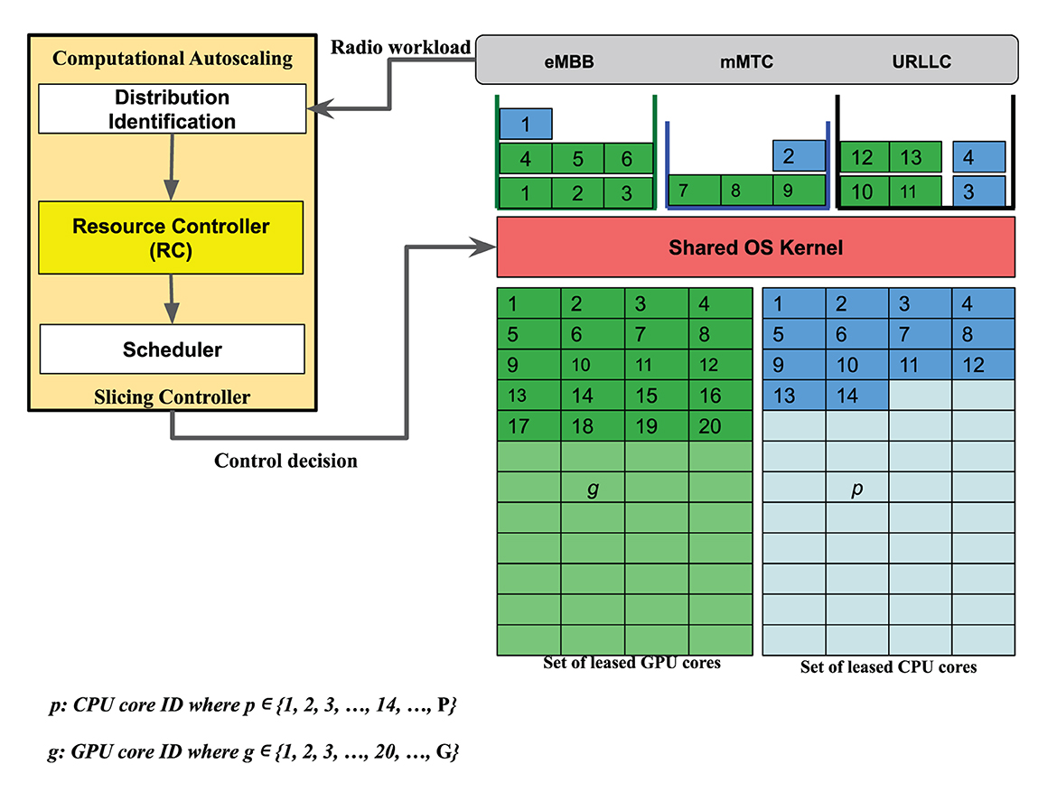
Figure 2. System model.

There is a set of computational resources $\mathcal{J}=\{\mathcal{P},\mathcal{G}\}$ where $\mathcal{P}=\left\{1,2,ldots,p,ldots,P-1,P\right\}$ is a set of CPU cores, and $\mathcal{G}=\left\{1,2,ldots,g,ldots,G-1,G\right\}$ a set of GPU cores to support a set of containers $\mathcal{I}$. There is a set of containers $\mathcal{I}=\left\{e,m,u\right\}$ where e, m, and u refer to eMBB, mMTC, and URLLC service categories, respectively. We define the containers' limits as l_i ∀ containers $i\in \mathcal{I}$ and ∀ resources $j\in \mathcal{J}$ where l_i = {l_ip, l_ig} for each container $i\in \mathcal{I}$, where l_ip, and l_ig represent allocated CPU cores or GPU cores to run the LDPC radio function in a container i, respectively. We define c_ij as the cost of using a computational resource $j\in \mathcal{J}$ to process workload in a container $i\in \mathcal{I}$. The cost c_ij = [c_ip, c_ig] is defined per allocated resource unit, where c_ip, and c_ig define the cost of using a CPU core p, and GPU core g to support a container i, respectively.

2.1.2.4. Design requirements

RAN slicing defines several design metrics to specify a service level agreement (SLA) between MVNOs and infrastructure providers, e.g., availability, latency, reliability, security, and throughput. However, we focus on latency and isolation design requirements. We consider isolation among resources since it is critical to achieving security requirements. Latency is modeled as a design constraint where the processing delay $\widetilde{{\tau }_i}$ is less than a pre-defined threshold δ_i for each container i ∈ $\mathcal{I}$. We model the isolation at the hardware level by assigning a resource j ∈ $\mathcal{J}$ to a container i ∈ $\mathcal{I}$ where j is not used by any other container in ${\mathcal{I}}^{‘}$ ⊂ $\mathcal{I}$ where ${\mathcal{I}}^{‘}=\mathcal{I}-i$. We assume that the isolation requirement at the OS kernel level is achieved by other methods such as Van't Hof and Nieh (2022).

2.2. Autoscaling methods

2.2.1. Problem statement

The core concept of RAN slicing is auto-scaling resources to deliver on-demand virtual network environments for various use cases. This research investigates the capability of RC to auto-scale MEC resources without HS deployment where resource limits are removed from the containers' configuration and determined as outcomes of the RC decision-making process. In this sense, we aim to minimize the cost of running slices where a limited amount of computational resources are allocated to process demands with random fluctuations such that an SLA is fulfilled, i.e., the processing delay is maintained below a pre-defined threshold δ_i. Figure 2 depicts the modeling of computing resources as items packed into LDPC containers (bins). Bin sizes, i.e., l_i, are outcomes of the RC decision-making process. Hence, RC is defined as a problem of packing resources into containers where an SLA is satisfied with minimum cost.

2.2.2. Problem formulation

We formulate the resource limit decision-making problem as a variant of the classical bin packing problem (BPP) (Johnson, 1973) where a MVNO has a fixed number of bins (i.e., containers) that have variable sizes, which depend on the amount of allocated resources (i.e., items) to meet the variations in workload (i.e., demands). Therefore, we need to determine the optimal size l_i of each container $i\in \mathcal{I}$ to minimize the total cost of running containers and meet SLA requirements (i.e., processing time $\widetilde{{\tau }_i}$ below the pre-defined threshold δ_i and resources per container are isolated). To determine l_i, we define a binary decision variable x_ij = [x_ip, x_ig] that equals 1 when a resource j is assigned to a container i and equals 0 otherwise. Thus, $l_i=\sum _{j\in \mathcal{J}}{x}_{ij}=\left\{l_{ip},l_{ig}\right\}$ where $l_{ip}=\sum _{p\in \mathcal{P}}{x}_{ip}$ and $l_{ig}=\sum _{g\in \mathcal{G}}{x}_{ig}$ $\forall i\in \mathcal{I}$.

The objective is to minimize the cost of running containers. Since we define the cost c_ij to use resource j for a container i, the cost function is formulated as follows.

$\begin{array}{ll}{\displaystyle \sum _{i\in I}}{\displaystyle \sum _{j\in J}}{x}_{ij}{c}_{ij}={\displaystyle \sum _{i\in I}}{\displaystyle \sum _{p\in P}}{x}_{ip}{c}_{ip}+{\displaystyle \sum _{i\in I}}{\displaystyle \sum _{g\in G}}{x}_{ig}{c}_{ig}& (1)\end{array}$

Since we process a container $i\in \mathcal{I}$, which runs the LDPC decoding algorithm, by using either CPU cores or GPU cores for minimum cost, we formulate processing time design constraints for each container $i\in \mathcal{I}$ as follows.

$\begin{array}{ll}\widetilde{{\tau }_{ip}}\le {\delta }_{i}or\widetilde{{\tau }_{ig}}\le {\delta }_i\forall i\in I\forall p\in P\forall g\in G& (2)\end{array}$

Here, $\widetilde{{\tau }_{ip}}=\frac{\tilde{R}.OP{S}_i^d}{\sum _{p\in \mathcal{P}}{x}_{ip}.min({\pi }_p,{\beta }_{p}A)}$, and $\widetilde{{\tau }_{ig}}=\frac{\tilde{R}.OP{S}_i^d}{\sum _{g\in \mathcal{G}}{x}_{ig}.min({\pi }_g,{\beta }_{g}A)}$. $OP{S}_i^d$ and A are first-order approximations of arithmetic operations and arithmetic operational intensity of the LDPC decoding algorithm that runs in a container $i\in \mathcal{I}$, respectively. π_p and π_g are the peak performance of CPU and GPU architectures, respectively. β_p and β_g are the memory bandwidth of the CPU and GPU, respectively.

To guarantee that a resource j can only be used at most once by a container i, we formulate the isolation design constraint as follows.

$\begin{array}{ll}{\displaystyle \sum _{i\in I}}{x}_{ij}\le 1\forall j\in J& (3)\end{array}$

We also have resource constraints as follows.

$\begin{array}{ll}{\displaystyle \sum _{i\in I}}{\displaystyle \sum _{p\in P}}{x}_{ip}\le P& (4)\end{array}$

$\begin{array}{ll}{\displaystyle \sum _{i\in I}}{\displaystyle \sum _{g\in G}}{x}_{ig}\le G& (5)\end{array}$

Thus, the problem is formulated as follows.

$\begin{array}{c}\underset{{}_{x_{ij}}}{\text{min}}3l{\displaystyle {\sum }_{i\in ℐ}{\displaystyle {\sum }_{j\in J}{c}_{ij}{x}_{ij}}}\\ \text{s}.\text{t}.2\text{ through }5\\ x_{ij}\in \{0,1\}& (6)\end{array}$

The problem in Equation (6) is a variant of the stochastic bin packing problem (SBPP) with a non-linear stochastic processing time constraint in Equation (2) that results in an infeasible solution. Chance-constrained methods (Kall and Wallace, 1994) are adopted to approach the SBPP-based RC (S-RC) problem.

Equation (2) is written as “$\frac{\widetilde{R_i}.OP{S}_i^d}{{\delta }_i.\sum _{p\in \mathcal{P}}{x}_{ip}}\le min({\pi }_p,{\beta }_{p}A)or\frac{\widetilde{R_i}.OP{S}_i^d}{{\delta }_i.\sum _{g\in \mathcal{G}}{x}_{ig}}\le min({\pi }_g,{\beta }_{g}A)\forall i\in \mathcal{I}$”. However, $min({\pi }_p,{\beta }_{p}A)\ge \frac{\widetilde{R_i}.OP{S}_i^d}{{\delta }_i.\sum _{p\in \mathcal{P}}{x}_{ip}}$ is equivalent to ${\pi }_p\ge \frac{\widetilde{R_i}.OP{S}_i^d}{{\delta }_i.\sum _{p\in \mathcal{P}}{x}_{ip}}$ and ${\beta }_{p}A\ge \frac{\widetilde{R_i}.OP{S}_i^d}{{\delta }_i.\sum _{p\in \mathcal{P}}{x}_{ip}}$. Therefore, $min({\pi }_p,{\beta }_{p}A)\ge \frac{\widetilde{R_i}.OP{S}_i^d}{{\delta }_i.\sum _{p\in \mathcal{P}}{x}_{ip}}$ is reformulated into $\widetilde{R_i}.OP{S}_i^d-{\pi }_p.{\delta }_i.\sum _{p\in \mathcal{P}}{x}_{ip}\le 0$ and $h_i.n_i.z-{\beta }_p.{\delta }_i.\sum _{p\in \mathcal{P}}{x}_{ip}\le 0$, $\forall i\in \mathcal{I}$ since $A=\frac{\widetilde{R_i}.OP{S}_i^d}{h_i.n_i.z}$. Likewise, $min({\pi }_g,{\beta }_{g}A)\ge \frac{\widetilde{R_i}.OP{S}_i^d}{{\delta }_i.\sum _{g\in \mathcal{G}}{x}_{ig}}$ is reformulated into $\widetilde{R_i}.OP{S}_i^d-{\pi }_g.{\delta }_i.\sum _{g\in \mathcal{G}}{x}_{ig}\le 0$ and $h_i.n_i.z-{\beta }_g.{\delta }_i.\sum _{g\in \mathcal{G}}{x}_{ig}\le 0$, $\forall i\in \mathcal{I}$. Furthermore, we introduce a new binary decision variable y_i to linearize the “or” operator where y_i = 1 for CPU and y_i = 0 for GPU resources to process the LDPC in container $i\in \mathcal{I}$. We also add another constraint, which uses y_i, to guarantee that the selection of CPU or GPU resources is associated with its resource limits $\sum _{p\in \mathcal{P}}{x}_{ip}$ or $\sum _{g\in \mathcal{G}}{x}_{ig}$, respectively. Therefore, Equation (2) is reformulated as follows.

$\begin{array}{ll}\widetilde{R_i}.OP{S}_i^d-{\pi }_p.{\delta }_i.{\displaystyle \sum _{p\in P}}x{y}_{ip}\le M_i(1-y_i)\forall i\in I& (7)\end{array}$

$\begin{array}{ll}\widetilde{R_i}.OP{S}_i^d-{\pi }_g.{\delta }_i.{\displaystyle \sum _{g\in G}}x{y}_{ig}\le M_i{y}_i\forall i\in I& (8)\end{array}$

$\begin{array}{ll}{h}_i.n_i.z-{\beta }_p.{\delta }_i.{\displaystyle \sum _{p\in P}}x{y}_{ip}\le M_i(1-y_i)\forall i\in I& (9)\end{array}$

$\begin{array}{ll}{h}_i.n_i.z-{\beta }_g.{\delta }_i.{\displaystyle \sum _{g\in G}}x{y}_{ig}\le M_i{y}_i\forall i\in I& (10)\end{array}$

$\begin{array}{ll}{\displaystyle \sum _{p\in P}}{x}_{ip}\le M_i{y}_i\forall i\in I& (11)\end{array}$

$\begin{array}{ll}{\displaystyle \sum _{g\in G}}{x}_{ig}\le M_i(1-y_i)\forall i\in I& (12)\end{array}$

Here, M_i is a large constant value that we choose to guarantee that constraints in Equations (7)–(12) are satisfied for any value of decision variable y_i, i.e., $M_i=max(P,G,(\widetilde{R_i}.OP{S}_i^d-{\pi }_p.{\delta }_i.P),(h_i.n_i.z-{\beta }_p.{\delta }_i.P),(\widetilde{R_i}.OP{S}_i^d-{\pi }_g.{\delta }_i.G),(h_i.n_i.z-{\beta }_g.{\delta }_i.G))$. Furthermore, we introduce xy_ip = x_ip.y_i, and xy_ig = x_ig.(1−y_i) as new non-linear binary decision variables to guarantee resource allocation for the selected resource, i.e., CPU or GPU. Thus, we add the following constraints for linearization purposes.

$\begin{array}{ll}x{y}_{ip}\le y_i\forall i\in I\forall p\in P& (13)\end{array}$

$\begin{array}{ll}x{y}_{ip}\le x_{ip}\forall i\in I\forall p\in P& (14)\end{array}$

$\begin{array}{ll}x{y}_{ip}\ge x_{ip}+y_i-1\forall i\in I\forall p\in P& (15)\end{array}$

$\begin{array}{ll}x{y}_{ip}\ge 0\forall i\in I\forall p\in P& (16)\end{array}$

$\begin{array}{ll}x{y}_{ig}\le 1-y_i\forall i\in I\forall g\in G& (17)\end{array}$

$\begin{array}{ll}x{y}_{ig}\le x_{ig}\forall i\in I\forall g\in G& (18)\end{array}$

$\begin{array}{ll}x{y}_{ig}\ge x_{ig}-y_i\forall i\in I\forall g\in G& (19)\end{array}$

$\begin{array}{ll}x{y}_{ig}\ge 0\forall i\in I\forall g\in G& (20)\end{array}$

Equations (7) and (8) introduce $\widetilde{R_i}$ as a Gaussian random variable where processing time constraints are expressed as probabilistic constraints that are fulfilled with probability α. Thus, Equations (7) and (8) are rewritten as $Pr(\widetilde{R_i}.OP{S}_i^d-{\pi }_p.{\delta }_i.\sum _{p\in \mathcal{P}}x{y}_{ip}\le M_i(1-y_i))\ge \alpha$ and $Pr(\widetilde{R_i}.OP{S}_i^d-{\pi }_g.{\delta }_i.\sum _{g\in \mathcal{G}}x{y}_{ig}\le M_i{y}_i)\ge \alpha$, $\forall i\in \mathcal{I}$, respectively. The probabilistic constraints are manipulated by using the definition of inverse cumulative distribution function (inverse-CDF) of Gaussian random variable $CD{F}_{\widetilde{R_i}}^{-1}(\alpha )$. Then, $Pr(\widetilde{R_i}\le {\zeta }_j)\ge \alpha$, where j∈{p, g}, is reformulated as $\zeta \ge CD{F}_{\widetilde{R_i}}^{-1}(\alpha )$, which can be written as ${\zeta }_j\ge \overline{R_i}+{\Phi }_{\widetilde{R_i}}^{-1}(\alpha ).{\sigma }_{R_i}$ where ${\zeta }_j=\frac{M_i{y}_{ij}+{\pi }_j.{\delta }_i.\sum _{j\in \mathcal{J}}x{y}_{ij}}{OP{S}_i^d}$; y_ij = y_i if j = p and y_ij = 1−y_i if j = g, $\overline{R_i}$ is the mean value of $\widetilde{R_i}$, σ_Ri is the variance of $\widetilde{R_i}$, and ${\Phi }_{\widetilde{R_i}}^{-1}(\alpha )=\sqrt{2}{\sigma }_{R_i}.er{f}^{-1}(2\alpha -1)+\overline{R_i}$ (Gilchrist, 2000) where erf⁻¹(2α−1) is the inverse error function of (2α−1). Accordingly, Equations (7) and (8) are rewritten as follows.

$\begin{array}{ll}{u}_i.OP{S}_i^d-{\pi }_p.{\delta }_i.{\displaystyle \sum _{p\in P}}x{y}_{ip}\le M_i(1-y_i)\forall i\in I& (21)\end{array}$

$\begin{array}{ll}{u}_i.OP{S}_i^d-{\pi }_g.{\delta }_i.{\displaystyle \sum _{g\in G}}x{y}_{ig}\le M_i{y}_i\forall i\in I& (22)\end{array}$

Here, $u_i=(\overline{R_i}+{\Phi }_{\widetilde{R_i}}^{-1}(\alpha ).{\sigma }_{R_i})$. Hence, the deterministic and linear formulation of 6 is written as shown below in Equation (23). Table 1 summarizes the notations used for the S-RC model and problem formulation.

$\begin{array}{r}\underset{{}_{x_{ij}}}{\text{min}}3l{\displaystyle {\sum }_{i\in ℐ}{\displaystyle {\sum }_{j\in J}{c}_{ij}{x}_{ij}}}\\ \text{s}.\text{t}.3\text{ through }5\\ 9\text{ through }20\\ 21\text{ through }22\\ x_{ij},y_i,x{y}_{ij}\in \{0,1\}& (23)\end{array}$

TABLE 1

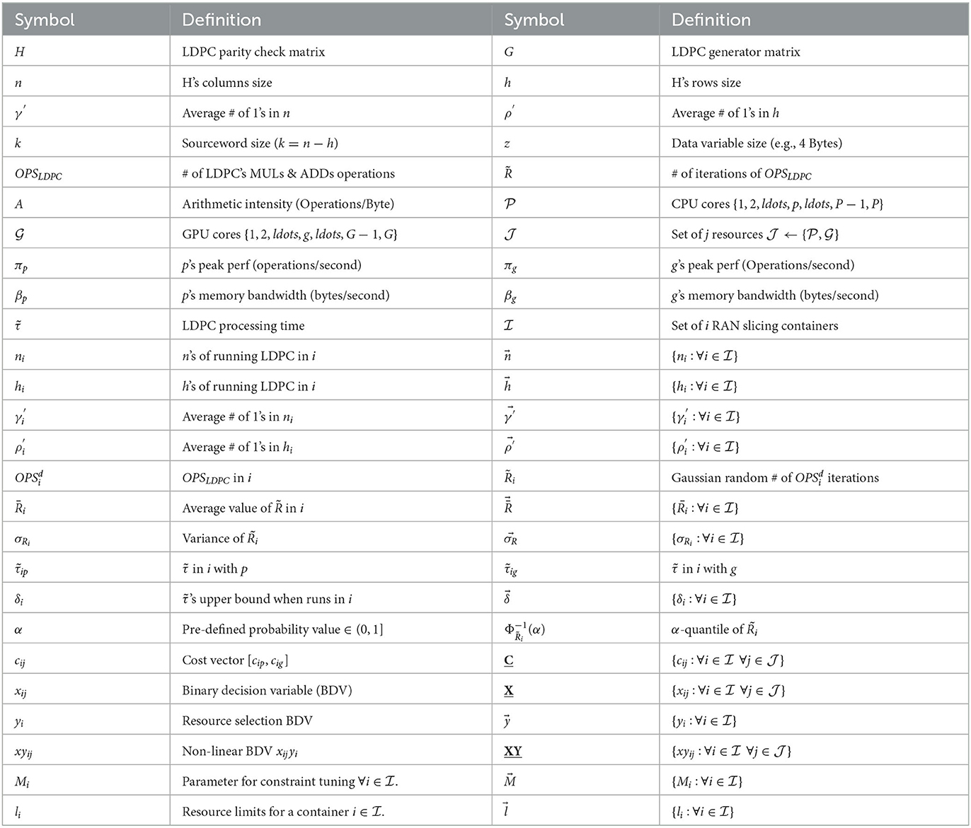
Table 1. List of symbols.

2.2.3. S-RC offline algorithm

Online algorithms for decision-making are often based on insights from their offline algorithms, (e.g., Fazi et al., 2012; Buchbinder et al., 2021; Foukas and Radunovic, 2021; Yan et al., 2022). In the following, we discuss the S-RC offline algorithm to determine each container's (i.e., RAN slice) optimal resource limits (l_i). As shown in Figure 2, there is a pre-processing stage that aims to identify the random distribution of radio workload patterns to determine $\overrightarrow{\overline{R}}$ and $\overrightarrow{{\sigma }_R}$. Then, the S-RC algorithm in Algorithm 1 initially computes the required data parameters for each slice category $i\in \mathcal{I}$, i.e., $OP{S}_i^d$, ${\Phi }_{{\tilde{R}}_i}^{-1}(\alpha )$, u_i, M_i. It then deploys Branch-and-Cut procedures to solve Equation (23). The Branch-and-Cut algorithm (B&C) (Mitchell, 2002) manages the complexity of Equation (23) by using the Branch-and-Bound B&B algorithm with the Cutting Plane algorithm (CP) (Wolsey, 2020). B&C is an iterative algorithm that uses B&B to partition the prior node (original problem) into two sub-nodes (subproblems) when we get a non-integer feasible solution of the relaxed LP. Then, the CP algorithm is called to find more linear constraints fulfilled by all feasible integers but violated by the current non-integer solution. This set of linear constraints is added to the problem, which leads to a new problem that is solved again as an LP problem using simplex methods. If the resulting solution is an integer and feasible, we compute the objective function of this integer solution and check for any other subproblems to be solved. If yes, B&B and CP iterate and the objective value with the new integer solution is inspected. If it is less than the last updated solution, it is chosen for the minimization problem. The process repeats until finding the optimal solution (Mitchell, 2002). Consequently, x_ij decision variables are determined by solving Equation (23), and, hence, optimal resource limits are obtained.

ALGORITHM 1

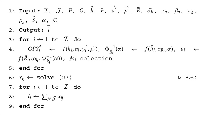
Algorithm 1. Offline S-RC.

3. Results

We evaluate the S-RC in the following. We describe the methodology and tool used for numerical evaluation and then discuss the numerical results.

3.1. Setup

To evaluate the S-RC, we consider the deployment of horizontal scaling (HS), where legacy RC uses pre-defined resource limits as a metric to instantiate a new container. Two performance metrics are defined for S-RC evaluation: (i) probability of processing time violation P_τ>δ; and (ii) S-RC cost overhead.

3.1.1. Performance metrics

The legacy RC enables HS to start a new container when a container's required resources surpass its pre-defined limits. However, HS deployment brings a critical question to our evaluation, which is “how could we set resource limits for each container (slice) according to the system setup that is described in Section 2”? To address this question, we define each container's resource limit as an average value $\overline{l_i}$, which is defined as $\overline{l_i}=\sum _{m=1}^k{p}_m{l}_{i_m}\forall i\in \mathcal{I}$ where p_m is the probability $Pr(R_{i_{m-1}}\le \widetilde{R_i}\le R_{i_m})$ and l_im is the solution of a deterministic instance of Equation (6), which is obtained by replacing the stochastic variable $\widetilde{R_i}$ with a deterministic value R_im where m = 1, 2, ldots, n, ldots, k. Following the same analysis and methods presented in Section 2, we obtain Equation (24) as shown below. Consequently, we use the resource limit computation algorithm in Algorithm 2 to solve Equation (24) with each sample of R_i∈{R_i1, ldots, R_im, ldots, R_ik} and determine l_im∈{l_i1, ldots, l_im, ldots, l_ik}.

$\begin{array}{ll}\begin{array}{l}\underset{{}_{x_{ij},x{y}_{ij},y_i}}{\text{min}}{\displaystyle \sum }_{i\in ℐ}{\displaystyle \sum }_{j\in J}{c}_{ij}{x}_{ij}\hfill \\ s.t.\hfill \\ 3through5\hfill \\ \hfill \\ 9through20\hfill \\ \hfill \\ R_{i_m}.OP{S}_i^d-{\pi }_p.{\delta }_i.{\displaystyle \sum }_{p\in }x{y}_{ip}\le M_i(1-y_i)\forall i\in ℐ\hfill \\ \hfill \\ R_{i_m}.OP{S}_i^d-{\pi }_g.{\delta }_i.{\displaystyle \sum }_{g\in G}x{y}_{ig}\le M_i{y}_i\forall i\in ℐ\hfill \\ \hfill \\ x_{ij},y_i,x{y}_{ij}\in \{0,1\}\hfill \end{array}& (24)\end{array}$

ALGORITHM 2

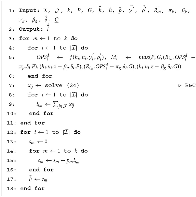
Algorithm 2. Resource limit computation with deterministic instants of $\tilde{R}$.

As mentioned above, we have two performance metrics to evaluate the S-RC. The first one is P_τ>δ, which is defined for S-RC as 1−α since we assume S-RC introduces a probabilistic time constraint that is fulfilled with a probability greater than α. Thus, the violation of the processing time design requirement occurs with chance (1−α), i.e., P_τ>δS−RC = 1−α. On the other hand, the legacy RC for HS deployment introduces an additional delay to start a container, which violates the processing time requirement if the required resources exceed the pre-defined resource limits. Therefore, $P_{{\tau >\delta }_{RC}}=Pr(R_{i_{m^{\prime }}}\le \widetilde{R_i}\le R_{i_{m^{″}}}|l_{i_{m^{″}}}>\overline{l_i})$ where $R_{i_{m^{\prime }}}$ is the deterministic m′ instant of $\widetilde{R_i}$ that satisfies $l_{i_{m^{\prime }}}<\overline{l_i}\le l_{i_{m^{\prime }+1}}$. Furthermore, $R_{i_{m^{″}}}$ is the deterministic m″ value of $\widetilde{R_i}$ that satisfies $l_{i_{m^{″}}}\ge l_{i_{m^{\prime }+1}}>\overline{l_i}$ where m″≥m′+1 and m′, m″∈{1, 2, 3, ..., k}. The second performance metric is the cost of running S-RC, which we define as the overhead cost percentage of the amount of resources used with S-RC and under-utilized with different values of R_im in legacy RC. Hence, S-RC cost overhead % $=\frac{(l_{i_{S-RC}}-l_{i_m}).Pr(\widetilde{R_i}\le R_{i_m})}{l_{i_m}}$ x 100%.

3.1.2. Experimental design

This paper adopts CPLEX C++ libraries (CPLEX and IBM ILOG, 2009) to implement Algorithms 1, 2 on Ubuntu 20.04.4 LTS that runs on Intel Core i5-8250U 8^thGen (1.6GHz x eight cores and 7.6 GiB RAM). We enumerate the set of containers $\mathcal{I}=\left\{1:eMBB,2:mMTC,3:URLLC\right\}$. Although each container deploys the same LDPC decoding algorithm, the processing time required for each category is different. We assume the processing delay requirement is δ_i = 0.3*RTD_i where RTD_i is the end-to-end round-trip delay (RTD) for each service category $i\in \mathcal{I}$ since edge cloud consumes about 30% of RTD to deliver eMBB, mMTC, or URLLC service (Fitzek et al., 2020). However, we only consider the LDPC radio decoding function, which consumes 60% of processing time at the edge (Foukas and Radunovic, 2021). Therefore, δ_i = 0.3*0.6*RTD_i where RTD_eMBB, RTD_mMTC, and RTD_URLLC have ranges 5–50, 10–50, and 0.5–50 ms, respectively (3GPP, 2017). Accordingly, we set the processing delay threshold $\overrightarrow{\delta }=\left[{\delta }_{eMBB},{\delta }_{mMTC},{\delta }_{URLLC}\right]$ where δ_eMBB = 0.18*5 = 0.9 ms, δ_mMTC = 0.18*10 = 1.8 ms, and δ_eMBB = 0.18*1 = 0.18 ms. We assume that the MVNO leases resources with a cost for CPU resources c_ip = {eMBB:0.1, mMTC:0.08, URLLC:0.05} and for GPU resources c_ig = {0.5, 0.4, 0.25} unit cost per unit time.

We assume five different data inputs, $(\overrightarrow{h},\overrightarrow{n},\overrightarrow{{\gamma }^{\prime }},\overrightarrow{{\rho }^{\prime }})$, to evaluate the impact of LDPC workload variations where D_wi values are $(h_i=100,...,500,n_i=200,...,1000,{\gamma }_i^{\prime }=34,...,170,{\rho }_i^{\prime }=68,...,340)\forall i\in \mathcal{I},w=1,2,3,4,5$, with step size 100, 200, 34, 68, for $h_i,n_i,{\gamma }_i^{\prime },{\rho }_i^{\prime }$, respectively. We set the average value of iterations $\overline{R_i}=15$ and the variance σ_Ri = 4 $\forall i\in \mathcal{I}$. For deterministic values of R_im, k is 10 with step size 5, i.e., R_im = 5, 10, ..., 45, 50. To study the impact of relaxing the probabilistic processing time constraint on resource limits, we consider different values of α where α = {0.5, 0.6, 0.7, 0.8, 0.9, 0.99}.

We consider running an LDPC on a cluster that uses the AMD EPYC 7251 processor architecture. Although the EPYC 7251 has eight cores, we assume the number of cores for our model is 64 cores, i.e., P = 64 (AMD, 2006) with the number of integer operations π_b = 5.954GigaOperations/s per core and its memory bandwidth per socket β_p = 153.6 GB/s (PassMark Software, 2018). Moreover, the cluster has NVIDIA Volta Tesla V100 GPU architecture that has 640 cores, i.e., G = 640, and 112 Tera Flops for tensor operations, i.e., matrix multiplication operations, i.e., π_g = 175GigaOperations/s, and memory bandwidth β_g = 900 GB/second (NVIDIA, 2018).

To measure the value of P_τ>δ, we run 50 experiments with different deterministic samples of R_im (10 R_ims x 5 data inputs) to evaluate the legacy RC for HS deployment where each container's resource limit is determined as described in Algorithm 2. Then, we run five experiments (5 data inputs) of Algorithm 1 to measure the overhead cost of running S-RC. In both sets of experiments, we set α = 0.99 for S-RC. Following that, we study the impact of α on resource limit per container type by running 30 experiments of S-RC with different values of α (i.e., 6 αs × 5 data inputs). We share CPLEX models of Algorithms 1, 2 on GitHub (Mazied, 2022). The following subsection discusses results.

3.2. Numerical evaluation

Figures 3–7 illustrate the impact of data size on the processing time violation and overhead cost for each service category (i.e., container type). The legacy RC for HS deployment does not violate the processing time requirement with a tiny data size, as shown in Figure 3A. However, Figures 6A, 7A show that S-RC performs better than RC for all containers with large and enormous data sizes. Nevertheless, RC for HS deployment violates the processing time required for limited data size with only a URLLC container as shown in Figure 4A due to its strict processing time requirement, i.e., δ_URLLC is the lowest threshold value of 0.18 ms. Figures 4–7 show that as data size grows, the number of containers that violate the processing time requirement increases due to HS deployment, which imposes starting new containers to satisfy the growing demands for LDPC processing. Furthermore, the excess in P_τ>δ for HS deployment occurs when R_m>15, which is greater than the average value of LDPC iterations ${\overline{R}}_{S-RC}$. On the other hand, S-RC shows higher overhead cost due to allocating more resources than what is instantaneously consumed with different values of R_m>15, in particular, Figures 3B, 4B, 5B, 6B show the highest overhead cost for URLLC containers that have strict processing requirements with average 75%, 58%, 60%, and 63%, respectively. However, Figure 7B shows that URLLC has only 51% average overhead cost, which is the lowest among other scenarios of lower data size, because of allocating only 2 GPU cores for LDPC operations in this scenario. Nevertheless, the trend of URLLC overhead will vary if we assume a higher cost for GPU allocation. In our setup, we assume GPU cost is 0.25 unit cost per unit time, while CPU cost is 0.05 unit cost per unit time for the URLLC container. We observe that overhead cost ranges from 0 to 200% with an overall average, for all data input sets and containers, of approximately 45%, which is foreseen as a relatively low average overhead for achieving low processing time requirements with high probability. Nevertheless, overhead costs in this case study reflect the limitation of using exact algorithms, i.e., B&C, that provide the optimal solution for combinatorial problems. Therefore, we are motivated to develop approximation algorithms that would provide a near-optimal solution for combinatorial problems, (e.g., D'Oro et al., 2020), with minimum overhead costs overhead. Table 2 summarizes the average overhead cost for each slice category and data input.

FIGURE 3

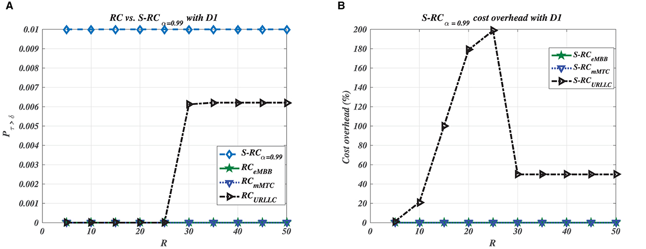
Figure 3. Tiny data size D₁. (A) Time violation. (B) Cost overhead.

FIGURE 4

Figure 4. Limited data size D₂. (A) Time violation. (B) Cost overhead.

FIGURE 5

Figure 5. Modest data size D₃. (A) Time violation. (B) Cost overhead.

FIGURE 6

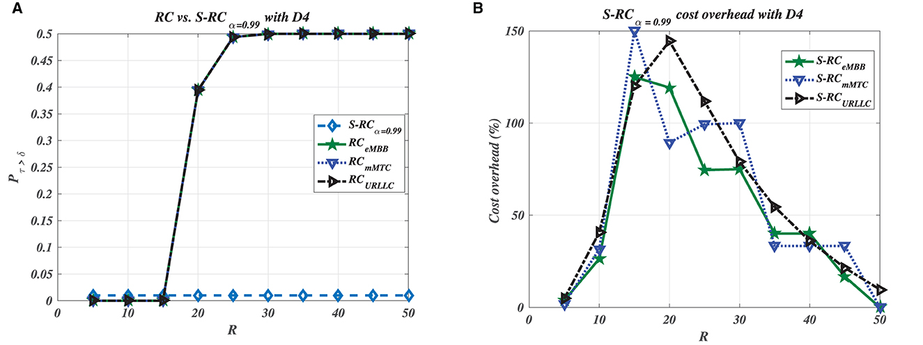
Figure 6. Large data size D₄. (A) Time violation. (B) Cost overhead.

FIGURE 7

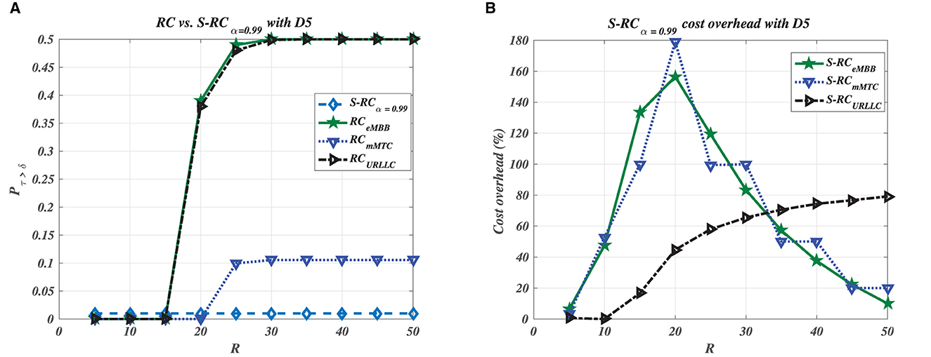
Figure 7. Enormous data size D₅. (A) Time violation. (B) Cost overhead.

TABLE 2

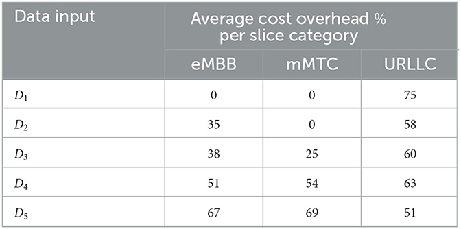
Table 2. Average overhead cost of using S-RC.

Figure 8 depicts the impact of selecting α, with different data input sizes, on the resource limits c_α and g_α (i.e., number of allocated resources) that refer to CPU and GPU resource limits, respectively. Figures 8A, B show that relaxing the processing time constraint with a probability 0.5 ≤ α ≤ 0.99 does not affect resource limits for containers that have a low delay threshold with tiny and limited data sizes (i.e., data input D₁, D₂, and D₃ in eMBB and mMTC containers). However, enormous data sizes in eMBB and mMTC containers show slight changes in resource limits due to tuning α. On the other hand, Figure 8C demonstrates significant increments in resource limits due to tuning α, in particular with enormous data size (D₅) where S-RC allocates 2 GPU cores for α = 0.99.

FIGURE 8

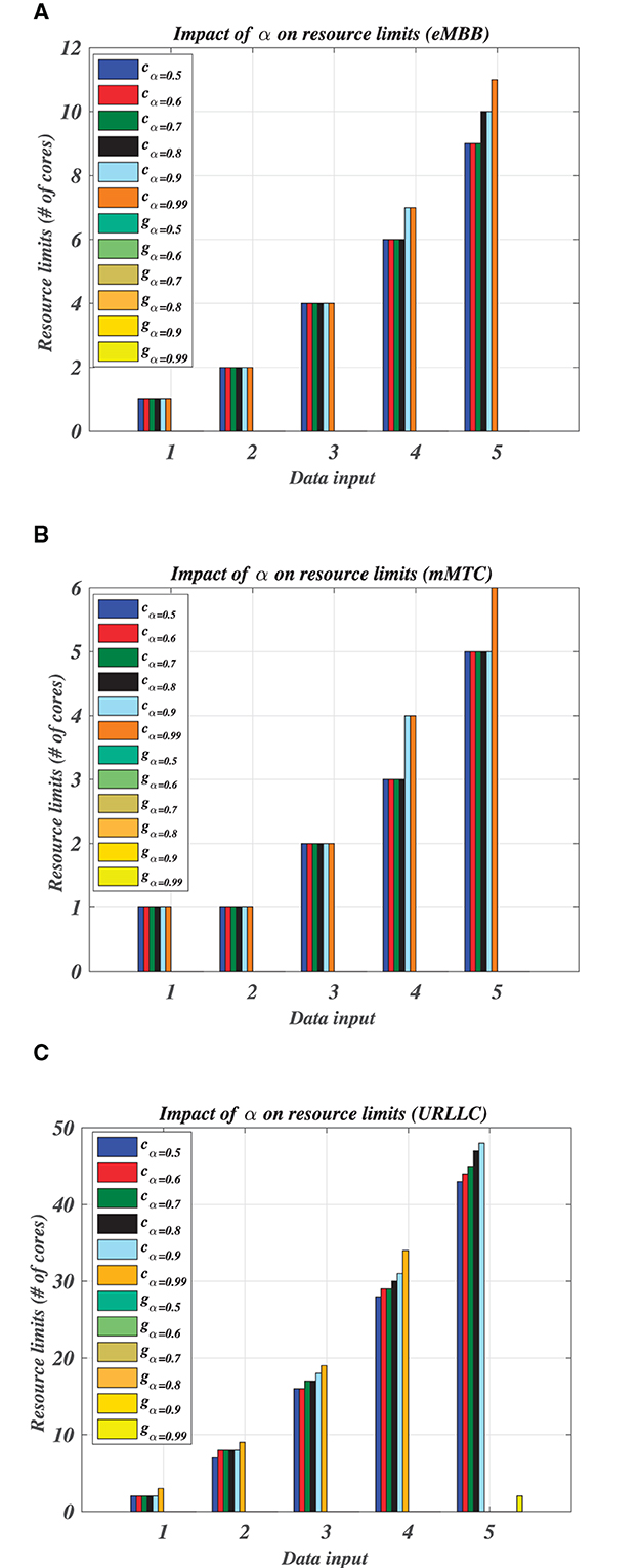
Figure 8. Impact of α on resource limit l_i. (A) eMBB resource limits. (B) mMTC resource limits. (C) URLLC resource limits.

4. Discussion

The results presented in Section 3 show that S-RC deployment has a high likelihood to effectively auto-scale the edge cloud for RAN slicing workload. However, its deployment cost, especially with containers with large data sizes and low latency requirements (i.e., URLLC container), is high due to using an exact method to solve the S-RC problem. Furthermore, in MEC, it is essential to utilize resources efficiently. Thus, S-RC could be augmented to achieve better resource usage by developing approximation algorithms for the introduced offline S-RC and developing an online algorithm for real-time operation.

The core concept of S-RC design is workload characterization (i.e., workload pattern identification). While the characterization of the RAN slicing workload is still challenging, inspecting MEC resource usage for containerized radio workloads with strict processing time requirements is critical for S-RC design. The inspection would deliver improved workload pattern recognition with a more accurate random distribution of its variations. Furthermore, auto-scaling the edge requires the optimal estimation of the scaling period since real-time autoscaling depends on capturing the variations in workload characteristics to scale up/down the resources. Indeed, a low scaling period would lead to a more accurate workload characterization. However, there is a tradeoff between scaling period determination and the required time for online resource allocation and scheduling decision-making. Therefore, RAN slicing workload characterization is mandatory for a practical S-RC design, especially if we get a periodic pattern of workload variations that could be leveraged to determine the optimal scaling period and workload distribution at the edge.

Resource selection is another crucial factor for S-RC design. This paper presents a rudimentary S-RC model, which decides the resource type based on resource usage value, i.e., selects CPU or GPU according to minimization of the cost function. Since our model assumes CPU cost is much lower than GPU cost, the B&C algorithm always selects the resource with lower cost, provided that linear design constraint is fulfilled. Nevertheless, resource selection should consider other performance metrics affecting the MEC's overall performance for RAN slicing production, such as memory access time and energy consumption.

Accordingly, S-RC can be deployed for delay-sensitive applications, including RAN slicing workloads, by considering the workload characterization and S-RC algorithmic development design factors.

4.1. Workload characterization

Instead of introducing a case study, i.e., LDPC radio function, to characterize the workload, hardware profiling tools such as PERF (WiKi, 2023) can be used for distribution identification (pattern recognition) of realistic workloads. Hardware profiling tools would facilitate the measurement of arithmetic intensity A, resource usage, task execution time, and many other performance metrics that read processing and memory counters of different traces of radio workload. Moreover, to model the processing time constraint in the introduced S-RC algorithm, an extended Roofline model (Cabezas and Püschel, 2014) can be constructed using an LLVM tool (LLVM Project, 2023) to define the peak performance of the underlying architecture with various traces of input data that reflect the fluctuations in use-cases' activities in the wireless environment. Furthermore, the characterization study would highlight the frequency of workloads variations that necessitate running autoscaling algorithms.

4.1.1. Algorithmic development

Since the S-RC design is still in its infancy, three stages should follow what this work introduces–first, developing a scaling period optimization algorithm that would rely on the outcomes of the workload characterization study. Then, an approximation offline algorithm for the S-RC would be developed to minimize the overhead cost of using the B&C algorithm. Following that, motivated by seminal works in Ayala-Romero et al. (2019), Buchbinder et al. (2021), and Foukas and Radunovic (2021), the development of an online S-RC algorithm becomes critical for production phase where heuristic/machine learning tools could be introduced to augment the results of the S-RC offline approximation algorithm.

5. Conclusion

Autoscaling mobile edge computing (MEC) is at the core of the radio access network (RAN) slicing operation since it tailors MEC resources to fulfill variations in demands for different wireless communication services. Autoscaling the edge takes place by either scaling resources (vertical) or scaling the number of containers (slices) for each service category (horizontal). When the demands for MEC resources exceed predefined resource limits, horizontal scaling (HS) incurs an additional 0.5 to 5 second delay to start a new container for the RAN slicing operation, which violates the strict timing requirements for radio processing, i.e., 0.5–50 ms. This paper introduces a design of a resource control (RC) decision-making process to scale the MEC resource without HS deployment, thus, eliminating HS delay. We develop stochastic RC (S-RC) where resource limits are removed from container configuration files and determined as outcomes of the S-RC decision-making process. S-RC is modeled as an offline stochastic bin packing problem where MEC resources (items) need to be packed into containers (bins) according to stochastic variations in RAN slicing workloads (demands). As a case study, the Low-Density Parity Check (LDPC) decoding algorithm is used to model radio workload, and the Roofline model is adopted to model the MEC performance. LDPC asymptotic analysis and the Roofline model are leveraged for deriving processing time design constraints where LDPC stochasticity lies in the random distribution of LDPC iterations. Stochastic and combinatorial optimization methods are utilized to decide resource limits for each container type in the S-RC problem. Although S-RC outperforms the legacy RC for HS deployment in terms of meeting processing time requirements, it experiences resource underutilization overhead compared to the deterministic alternative of the S-RC, where deterministic samples of LDPC iterations replace its inverse cumulative distribution function for processing time design constraint. Developing an approximation algorithm for the offline S-RC could subside overhead cost.

We plan to characterize RAN slicing workload with complete consideration of radio functions and realistic operational scenarios to augment the S-RC design. Workload characterization would identify workload fluctuation patterns and determine the optimal scaling period for online S-RC design.

Data availability statement

The original contributions presented in the study are included in the article/supplementary material, further inquiries can be directed to the corresponding authors.

Author contributions

EM conceived of soft-tuning resource limits as outcomes of the decision-making process rather than hard coding them as user-defined configurations, developed the system model and formulated the problem, conducted the experiments and designed the performance metrics for numerical evaluation, discussed the obtained results and concluded the research by drawing directions for future work, and wrote the paper and followed the co-authors' instructions for its organization and presentation style. DN suggested developing the processing time design constraint using algorithmic asymptotic analysis and Roofline model and advised EM through paper development, and made the necessary edits. YH reviewed the paper during its initial development phase and suggested highlighting the research question at the very beginning of the paper and comparing the results using different data inputs to reflect the impact of workload variations on system performance. SM revised the initial draft of the paper, suggested its organization and presentation style, suggested presenting a table to summarize the mathematical notations of the system model and problem formulation, and advised EM through paper development. All authors contributed to the article and approved the submitted version.

Funding

We acknowledge the funding from the Virginia Tech office of Research and Innovation for their grant Fellowship for Graduate Student First-Author Papers.

Conflict of interest

DN declared that they were an editorial board member of Frontiers, at the time of submission. This had no impact on the peer review process and the final decision.

The remaining authors declare that the research was conducted in the absence of any commercial or financial relationships that could be construed as a potential conflict of interest.

Publisher's note

All claims expressed in this article are solely those of the authors and do not necessarily represent those of their affiliated organizations, or those of the publisher, the editors and the reviewers. Any product that may be evaluated in this article, or claim that may be made by its manufacturer, is not guaranteed or endorsed by the publisher.

Footnotes

1. ^Fading wireless channels introduce errors in received messages that mandate carrying out a random number of LDPC iterations for error detection/correction.

References

3GPP (2017). Evolved Universal Terrestrial Radio Access (E-UTRA); Radio Resource Control (RRC); Protocol specification. Technical Specification (TS) 36.331, 3rd Generation Partnership Project (3GPP). Available online at: https://portal.3gpp.org/desktopmodules/Specifications/SpecificationDetails.aspx?specificationId=2440

Google Scholar

3GPP (2018). Telecommunication Management; Study on Management and Orchestration of Network Slicing for Next Generation Network. Technical report.

Google Scholar

Akman, A., Li, C., Ong, L., Suciu, L., Sahin, B. Y., Li, T., et al. (2020). O-RAN Use Cases and Deployment Scenarios: Towards Open and Smart RAN. Technical report, O-RAN Alliance.

Google Scholar

AMD (2006). AMD EPYC 7251.

Google Scholar

Armbrust, M., Fox, A., Griffith, R., Joseph, A. D., Katz, R. H., Konwinski, A., et al. (2009). Above the Clouds: A Berkeley View of Cloud Computing. Technical report UCB/EECS-2009-28, Electrical Engineering and Computer Sciences University of California at Berkeley.

PubMed Abstract | Google Scholar

Ayala-Romero, J. A., Garcia-Saavedra, A., Gramaglia, M., Costa-Perez, X., Banchs, A., Alcaraz, J. J. (2019). “VrAIn: a deep learning approach tailoring computing and radio resources in virtualized RANs,” in Proc. ACM MobiCom (Los Cabos), 1–16.

Google Scholar

Bae, J. H., Abotabl, A., Lin, H.-P., Song, K.-B., Lee, J. (2019). “An overview of channel coding for 5G NR cellular communications,” in APSIPA Transactions on Signal and Information Processing, eds S. Furui, C.-C. Jay Kuo, and K. J. Ray Liu (Cambridge Press), 1–14. doi: 10.1017/ATSIP.2019.10

CrossRef Full Text | Google Scholar

Buchbinder, N., Fairstein, Y., Mellou, K., Menache, I., Naor, J. (2021). Online virtual machine allocation with lifetime and load predictions. ACM Sigmetr. Perform. Eval. Rev. 49, 9–10. doi: 10.1145/3543516.3456278

CrossRef Full Text | Google Scholar

Cabezas, V. C., Püschel, M. (2014).15 “Extending the roofline model: bottleneck analysis with microarchitectural constraints,” in Proc. of the IEEE 15th IISWC (Raleigh, NC), 222–231.

Google Scholar

Chandrasetty, V. A., Aziz, S. M. (2018a). “Chapter 2: Overview of LDPC codes,” in Resource Efficient LDPC Decoders, eds V. A. Chandrasetty and S. M. Aziz (Academic Press), 5–10.

Google Scholar

Chandrasetty, V. A., Aziz, S. M. (2018b). “Chapter 4: LDPC decoding algorithms,” Resource Efficient LDPC Decoders, eds V. A. Chandrasetty and S. M. Aziz (Academic Press), 29–53.

Google Scholar

CPLEX and IBM ILOG (2009). V12. 1: User's manual for CPLEX. Int. Bus. Mach. Corp. 46, 157. Available online at: https://www.ibm.com/docs/en/icos/12.8.0.0?topic=cplex-users-manual

Google Scholar

D'Oro, S., Bonati, L., Restuccia, F., Polese, M., Zorzi, M., Melodia, T. (2020). “Sl-edge: network slicing at the edge,” in Proc. of the ACM 21st MobiHoc, Mobihoc '20, 1–10.

Google Scholar

Fazi, S., Van Woensel, T., Fransoo, J. C. (2012). A stochastic variable size bin packing problem with time constraints. Eindhoven: Technische Universiteit Eindhoven, 382.

Google Scholar

Fitzek, F., Granelli, F., Seeling, P. (2020). Computing in Communication Networks: From Theory to Practice. Amsterdam: Academic Press.

PubMed Abstract | Google Scholar

Foukas, X., Radunovic, B. (2021). “Concordia: teaching the 5g vran to share compute,” in Proceedings of the 2021 ACM SIGCOMM 2021 Conference, 580–596.

Google Scholar

Garcia-Morales, J., Lucas-Estañ, M. C., Gozalvez, J. (2019). Latency-sensitive 5G RAN slicing for industry 4.0. IEEE Access 7, 143139–143159. doi: 10.1109/ACCESS.2019.2944719

CrossRef Full Text | Google Scholar

Gilchrist, W. (2000). Statistical Modelling with Quantile Functions. Chapman and Hall/CRC.

Google Scholar

Google (2022). Vertical Pod Autoscaling.

Google Scholar

Hamidi-Sepehr, F., Nimbalker, A., Ermolaev, G. (2018). “Analysis of 5G LDPC codes rate-matching design,” in 2018 IEEE 87th Vehicular Technology Conference (VTC Spring) (Porto: IEEE), 1–5.

Google Scholar

Henderson, D. (2022). Kubernetes CPU Throttling: The Silent Killer of Response Time—and What to Do About It. Available online at: https://community.ibm.com/community/user/aiops/blogs/dina-henderson/2022/06/29/kubernetes-cpu-throttling-the-silent-killer-of-res

Google Scholar

Johnson, D. S. (1973). Near-optimal bin packing algorithms (Ph.D. thesis). Massachusetts Institute of Technology, Cambridge, MA, United States.

Google Scholar

Kall, P., Wallace, S. W. (1994). Stochastic Programming. John Wiley and Sons.

Google Scholar

Khun, E. (2020). Kubernetes: Make Your Services Faster by Removing CPU Limits. Available online at: https://erickhun.com/posts/kubernetes-faster-services-no-cpu-limits/

Google Scholar

Liu, Q., Han, T., Moges, E. (2020). “EdgeSlice: slicing wireless edge computing network with decentralized deep reinforcement learning,” in Proc. of the IEEE 40th ICDCS, ICDCS '20 (Singapore), 234–244.

Google Scholar

LLVM Project (2023). The LLVM Compiler Infrastructure.

Google Scholar

Maguolo, F., Mior, A. (2008). “Analysis of complexity for the message passing algorithm,” in 2008 16th International Conference on Software, Telecommunications and Computer Networks (Split), 295–299.

Google Scholar

Mazied, E. A. (2022). CPLEX Model of Stochastic Offline Resource Control for MEC Autoscaling. Available online at: https://github.com/emazied80/Stochastic_Resource_Control_to_AutoScale_MEC

Google Scholar

Microsoft (2022). Azure Kubernetes Service.

Google Scholar

Mitchell, J. E. (2002). Branch-and-cut algorithms for combinatorial optimization problems. Handb. Appl. Opt. 1, 65–77.

Google Scholar

Musthafa, F. (2020). CPU Limits and Aggressive Throttling in Kubernetes. Available online at: https://medium.com/omio-engineering/cpu-limits-and-aggressive-throttling-in-kubernetes-c5b20bd8a718

Google Scholar

NVIDIA (2018). TESLA v100 Performance Guide.

Google Scholar

PassMark Software (2018). AMD EPYC 7251 CPU Benchmarks.

Google Scholar

Sharon, E., Ashikhmin, A., Litsyn, S. (2006). Analysis of low-density parity-check codes based on exit functions. IEEE Trans. Commun. 54, 1407–1414. doi: 10.1109/TCOMM.2006

CrossRef Full Text | Google Scholar

Van't Hof, A., Nieh, J. (2022). “{BlackBox}: a container security monitor for protecting containers on untrusted operating systems,” in 16th USENIX Symposium on Operating Systems Design and Implementation (OSDI 22) (Carlsbad, CA), 683–700.

Google Scholar

WiKi, P. (2023). Linux Profiling with Performance Counters. Available online at: https://perf.wiki.kernel.org/index.php/Main_Page

Google Scholar

Williams, S., Waterman, A., Patterson, D. (2009). Roofline: an insightful visual performance model for multicore architectures. Commun. ACM 52, 65–76.

Google Scholar

Wolsey, L. A. (2020). Integer Programming. John Wiley & Sons.

Google Scholar

Yan, J., Lu, Y., Chen, L., Qin, S., Fang, Y., Lin, Q., et al. (2022). “Solving the batch stochastic bin packing problem in cloud: a chance-constrained optimization approach,” in Proceedings of the 28th ACM SIGKDD Conference on Knowledge Discovery and Data Mining, KDD '22 (Washington, DC: Association for Computing Machinery), 2169–2179.

Google Scholar

Yan, M., Feng, G., Zhou, J., Sun, Y., Liang, Y-C. (2019). Intelligent resource scheduling for 5G radio access network slicing. IEEE Trans. Veh. Technol. 68, 7691–7703.

PubMed Abstract | Google Scholar

Yuan, Z., Muntean, G.-M. (2020). AirSlice: a network slicing framework for UAV communications. IEEE Commun. Mag. 58, 62–68.

Google Scholar