A laser–laser method for carbonate C and O isotope measurement, metrology assessment, and stratigraphic applications

The stable isotopic compositions of carbon and oxygen (δ¹³C_carb and δ¹⁸O_carb) measured from carbonates are widely used in geology, notably to reconstruct paleotemperatures and the secular evolution of the biogeochemical carbon cycle, to characterize limestone sediment diagenesis, and to provide chemostratigraphy records. The standard technique used since the mid-20th century to measure C and O isotopic ratios is based on a wet chemical acid digestion protocol in order to evolve CO₂ from carbonates—the latter being analyzed by mass spectrometry and, more recently, infrared spectroscopy. A newly developed laser-based method aims to circumvent this chemical preparation step by producing CO₂ via an instant and spatially resolved calcination reaction. We describe an evolution of the laser calcination benchtop system previously described and used as a proof of concept toward a portable system, and we present the efficiency of this tool for performing carbon and oxygen isotope measurements from carbonate matrixes following standard evaluation metrology protocol. This metrological study explores the following: i) the use of internal standards; ii) inter-calibration with the traditional acid chemical preparation method; iii) analysis of the uncertainties of using GUM and ANOVA. Using 15 different types of carbonate minerals encompassing a range of isotopic VPDB compositions between −18.6‰ and +16.06‰ and between −14.80‰ and −1.72‰ for δ¹³C_carb and δ¹⁸O_carb, we show that isotopic cross-calibration is verified for both carbon and oxygen, respectively, and we demonstrate that the uncertainties (1σ) of the δ¹³C_carb and δ¹⁸O_carb measurements of laser–laser isotopic analysis are within 0.41‰ and 0.68‰, respectively. The advantages of this method in saving time and spatially resolved and automated analysis in situ are demonstrated by high-resolution chemostratigraphic analysis of a laminated lacustrine travertine sample.

1 Introduction

Natural stable isotope ratios of carbonates (δ¹³C_carb and δ¹⁸O_carb) archived in the geological record are widely used to reconstruct local and global paleotemperatures and the secular evolution of the biogeochemical carbon cycle. They are routinely measured after several sample preparation steps that include (i) crushing or micro-drilling, (ii) transfer of sample powder into evacuated vials, and (iii) sample digestion using orthophosphoric acid (H₃PO₄; (McCrea, 1950)). The reaction time is generally between 15 min and 48 h, depending on the carbonate mineralogy. The CO₂ evolved is thereafter measured using classical isotope ratio mass-spectrometry (IRMS). While this entire process is long and time-consuming, it provides accurate values of δ¹³C_carb and δ¹⁸O_carb with typical internal reproducibility better than 0.1‰. Alternatively, very small sample volumes can be measured in situ using secondary ion mass spectrometry (SIMS) microanalysis. Measuring δ¹³C_carb and δ¹⁸O_carb through SIMS usually allows for a reproducibility in the range of 0.5‰–1‰ for a sample analysis spot-size of approximately 10 μm (e.g., Śliwiński et al., 2017). The preparation steps needed for accurate isotopic measurements with this method are numerous (e.g., embedding the sample with standards in epoxy mount, polishing to submicron level, cleaning, gold coating, etc.), and the chemical composition of the sample must be precisely and independently predetermined by electron probe microanalysis (EPMA) in order to correct for strong sample matrix effects. The analytical accuracy of SIMS δ¹⁸O and δ¹³C measurements is also affected by strong instrumental mass fractionation (e.g., Valley et al., 2009).

The recent development of a new generation of compact gas phase IRMS instruments based on technologies such as cavity ring-down spectroscopy (CRDS) or isotope-ratio infrared spectrometry (IRIS) has allowed the continuous and direct analysis of atmospheric CO₂ in field conditions without the need for complex purification (e.g., Garcia-Anton et al., 2014; Rizzo et al., 2014; Fischer and Lopez, 2016). The emergence of these smaller, lighter, portable optical mass spectrometer technologies has paved the way for an entirely new approach in carbon and oxygen isotopic measurements.

However, for carbonates, the need to couple gas measurements to an acid preparation line has impeded any field deployments with a dedicated field laboratory.

Consequently, we recently suggested that fiber-coupled laser diode-induced calcination can produce CO₂ out of carbonates without imparting fractionation to carbon isotopes and with a constant offset for oxygen compared to the acid digestion method (Thomazo et al., 2021). Fiber-coupled diode lasers are more highly compact than previous laser systems and can be paired with field-deployable CRDS/IRIS optical-mass spectrometers. This opens the possibility of analyzing carbonate carbon and oxygen isotope composition for spatially resolved isotopic characterization and for on-site or in-the-field measurements.

Hence, we present here an improved transportable setup for measuring stable isotope ratios in carbonates that consists of a homemade calcination system based on a fiber laser diode mounted on a small and easily transportable device paired to a commercial IRIS system. The evolved CO₂ gas produced after calcination is monitored for concentration and transfer efficiency to a commercial IRIS system via EXETAINER^® vials without further purification steps before the isotopic measurements. We demonstrate this analysis scheme on natural carbonates, discuss the accuracy and reproducibility of the method, compare its advantages with state-of-the-art dual inlet isotopic IRMS systems, and elaborate its potential future applications by exemplifying the method’s capabilities by high-resolution isotopic chemostratigraphy measurements of a finely laminated lacustrine travertine sample.

2 Materials and methods

The preparation and analysis of the carbonate samples were conducted in different laboratories: at the University of Burgundy, laser calcination was performed at the ICB Laboratory, and isotopic measurements using IRIS (ThermoScientific™ Delta Ray™) and conventional IRMS (ThermoScientific™ Delta V Plus™ IRMS coupled with a Kiel VI carbonate preparation device) methods at the Biogeosciences Laboratory. Finally, selected samples were analyzed using an Isoprime™ dual-inlet IRMS coupled with a MultiCarb™ carbonate preparation device at the Laboratory of Geology of Lyon (LGL-TPE). Different preparation and analysis methods were used and cross-calibrated to assess the robustness of the new laser–laser method and to assess the systematic errors of the different measuring and preparation devices.

2.1 Preparation methods

The isotopic analysis process comprised two steps. The first was the production of CO₂ from the rock, and the second corresponded to the analysis of the gas thus produced for its isotopic ratios. The conventional preparation step is based on acid digestion, while the new method, on a thermal transformation of carbonate into lime (CaO) and CO₂ using a laser as a heat source.

2.1.1 CO₂ production

2.1.1.1 Acid digestion preparation method

Acid digestion, the traditional method for measuring carbonates δ¹³C_carb and δ¹⁸O_carb (McCrea, 1950), is robust, precise, and provides external reproducibility for international standard analyses close to 0.1‰. This method needs several preparatory steps, including grinding or micro-drilling the sample to obtain between 50 and 100 µg (equivalent to calcite) of carbonate powder with a size of less than 140 µm. The powder obtained is transferred to glass vials where the air is evacuated and eventually replaced by a CO₂-free gas (for continuous flow system) and reacted with a 102% orthophosphoric acid (H3PO4) solution at a controlled temperature (from ambient to 70°C depending on the mineralogy of the carbonate) in order to convert C-bearing carbonate into CO₂. After the reaction, several additional steps to purify the gas produced are needed that may include removing other trace volatiles such as H₂O, CO, N₂, and Ar using condensation at liquid nitrogen temperature or gas chromatography.

2.1.1.2 Laser calcination method

Laser-induced calcination is essentially based on thermal light–matter interaction. Laser radiation is focused on a sample of carbonate (with a spot diameter in the focal plane of approximately 200 µm). The laser energy is absorbed by the sample (the carbonate and its impurities) and is then released in the form of heat. It is this local heating that allows the sample to reach the calcination threshold temperature and then produce the CO₂ used for the analysis (the details of the reaction are presented in Thomazo et al., 2021). Laser calcination can be performed under air, vacuum, synthetic air (without CO or CO₂), or even under a di-nitrogen atmosphere. These different working conditions do not affect the CO₂ production yield. The working pressure of this work was chosen at around atmospheric pressure.

2.1.2 Isotopic ratio CO₂ analyses

The CO₂, produced from the rock samples was analyzed by either sector field mass spectrometry or infrared optical spectrometry. These two methods used for the intercalibration and evaluation of the metrological performance of the new laser method are briefly presented below.

2.1.2.1 Sector field mass spectrometry

Two different dual-inlet IRMS carbonate analysis configurations were used in this study: a Kiel VI–Delta V Plus™ IRMS (Thermo Scientific™) and a MultiCarb™–GV Instrument Isoprime™ (Elementar™). In both cases, the CO₂ produced after orthophosphoric acid digestion is purified using a cryogenic trap at liquid nitrogen temperature before transfer by capillary tubing into the source (Nier type) of the mass spectrometers, where molecules are ionized. Accelerated by a strong difference of several thousands of volts, the ions are then deviated by a magnetic field and collected in Faraday cup type collectors. Samples are typically analyzed in a dual-inlet mode against an internal standard to provide the delta notation. This cycle of sample–standard analyses is reproduced ten times, and the software program provides the average value.

Measurement repeatability and accuracy were controlled by submitting the same treatment to aliquots of international standard for CaCO₃ (NBS19; δ¹³C_VPDB = +1.95‰ and δ¹⁸O_VPDB = −2.20‰). The internal uncertainty for the whole procedure using this protocol is typically below 0.03‰ for both δ¹³C_VPDB and δ¹⁸O_VPDB (1σ).

2.1.2.2 Optical infrared spectrometry

Optical isotopic analysis uses differentiated infrared absorption of the isotopes of C and O in the CO₂ molecules probed. This analysis is based on measuring the absorption coefficients of the specific fine infrared rays from which the respective concentrations are calculated. In this study, a commercial Delta Ray (Thermo Scientific™) infrared spectrometer that uses a mid-infrared laser operating at 4.3 μm wavelength was used. To obtain reliable and reproducible measurements, it was necessary to use reference gases, the measurement of which was used to calculate the isotopic ratios and estimate measurement precision. The reliable measurement of the isotopic ratios is subject to measurement drifts and errors of different sources. Therefore, a specific protocol alternating reference gas measurement and sample gas measurement was used. In this study, we measured the reference gas every five samples analyzed. The reference gas used in this study has isotopic values for δ¹³C_VPDB = $-25.5\pm 0.15$‰ and δ¹⁸O _VPDB = $-24.4\pm 0.15$‰ at 1 bar.

Following this protocol, the measurement uncertainty defined at the 1σ level by the manufacturer (considering the repeatability and precision of the device) was at 0.17‰ for δ¹³C and 0.18‰ for δ¹⁸O.

2.2 Sample descriptions

Because there is no certified carbonate carbon and oxygen isotopic standards have been developed for laser ablation analyses, we used in-house standards for cross-calibration and to verify the performance of the carbonate calcination technique. Some of the carbonate samples used have already been presented in Thomazo et al. (2021), and new samples were analyzed to broaden the range of isotopic compositions and improve the intercalibration and estimation of uncertainties. Table 1 presents the main characteristics of the samples used in this study.

TABLE 1

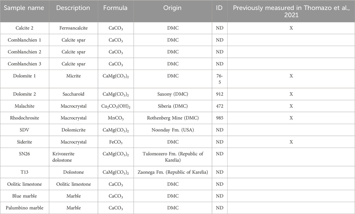
TABLE 1. Description of inhouse standards used for intercalibration and estimation of uncertainties during this study. Description: main lithological aspect. Formula: chemical formula of the considered carbonate. Origin: Dijon Museum Collection (DMC). ID, inventory number; ND, non-determined.

2.3 Detailed presentation of the laser preparation system

The initial system, working offline with the sample placed in a vacuum chamber, was used to demonstrate the feasibility of the method (Thomazo et al., 2021). In this study, we developed a new system that is i) compact and transportable, ii) “online” in the sense that the sample is in direct contact with the gas line, iii) working at atmospheric pressure with carrier gas, iii) fully automated, and iv) capable of mapping the samples.

Figure 1 presents a simplified scheme of the system. The three main subsystems are i) the optical and laser systems, ii) the gas circulation and control system, and iii) the electronic and operator control interface (hmi). All of these were integrated into a compact box frame (39 cm × 29 cm × 40 cm) with a mass of ∼14 kg (Figure 2). This box is easily transportable (with a handle) and can be put into operation as soon as an electrical source and gas supply (for example, nitrogen via a 6-mm port) are provided.

FIGURE 1

FIGURE 1. Scheme of the laser preparation system.

FIGURE 2

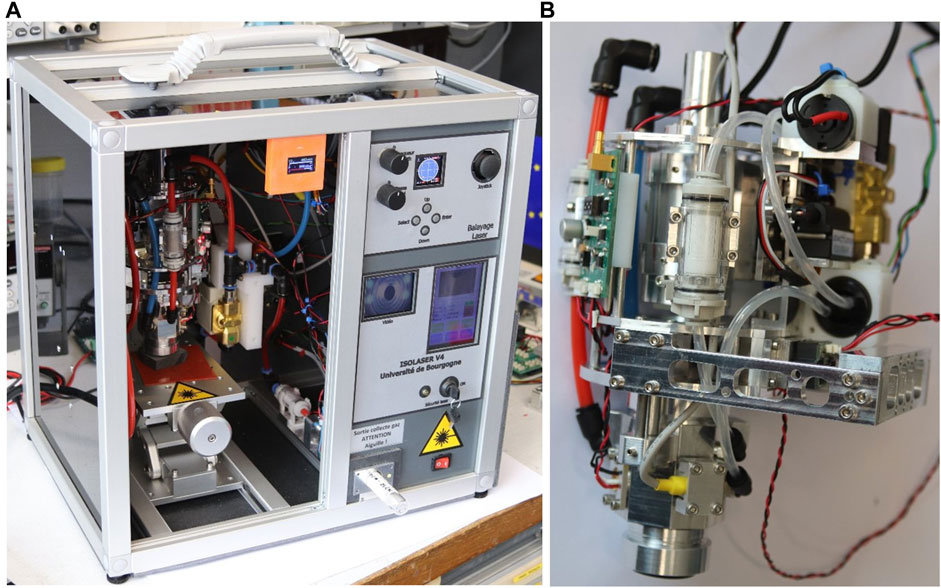
FIGURE 2. (A) Overview of the system integrated in an easily transportable box frame. (B) Detailed view of the optical head and gas chamber.

2.3.1 Control and power electronics

The laser source was a laser diode module with a maximum output power of 90 W and an emission wavelength of 915 ± 5 nm (Premier Photonics^®) connected to an optical fiber with 105-µm-diameter core and with a numerical aperture of 0.22. The laser module used is a commercial device dedicated to fiber laser pumping, manufactured in large series with low cost per optical watt. The optical-to-electrical efficiency of the laser module was 50% with a small volume factor (100 × 50 × 15 mm³). The laser source was temperature-controlled at 28°C using a Peltier module mounted on a heatsink. This stabilized both the operation in wavelength and the emission parameters (power and wavelength) independent of the environmental conditions. The output power of the laser was controlled by an adjustable power supply from 0 to 18 A, giving an output power between 0 and 90 W. The power module included the laser diode, power supply, Peltier driver, and two cooling fans and was connected to a single board Arduino Due computer. Several laboratory-made electronic boards and a color LCD touch screen allowed control of the setup's functions. The electronics were connected to the optical head and the gas line. The whole setup can be powered with a standard 24-V adapter or a battery (including a car battery) within a large input voltage range (from 9 to 36 V DC).

2.3.2 Optical head, gas line, and control interfaces

This sub-system included several functions dedicated to i) shaping the laser beam associated with a programmable mechanical two-axis displacement and imaging functions, ii) a reaction chamber including sensors, and iii) assistance and analysis of the gas circulation line.

2.3.2.1 Laser beam

The laser beam at the fiber output was shaped and focused on the sample by two achromats (50 and 100 mm, AC254-50-B and AC254-100-B, from Thorlabs ^®) with a focal length of approximately 100 mm corresponding to a laser spot of 200 μm in diameter and a depth of field (assuming ±10% variations of the diameter) of approximately ±1.0 mm. This telescope was mounted on a motorized displacement device comprising two linear servomotors (Actuonix^® PQ12-R-20-100:1) which allowed program raster analyses in a square of approximately 15 mm. This device was controlled by a joystick, two trimmers, and a four-key keyboard that allowed the controlling position and speed of the displacement with a typical resolution of 100 µm. A single board Arduino^® Uno computer with an LCD screen served as the user interface. Under the telescope was placed an IR/visible @45° dichroic mirror (64449 Edmund^®). A camera associated with a white LED lighting ring allowed visualization of the sample and the laser spot. An adjustable 16-mm lens also provided a high-definition image of the sample surface. This optical configuration of the alignment between the sight and the calcination point on the sample eliminated misalignment issues.

2.3.2.2 Gas calcination chamber

A small calcination chamber (23 cm³) was placed directly in contact with the sample via a conical O-ring seal (27 mm outer diameter). The sample was dry and flattened beforehand in order to ensure a tight connection with the sealing ring and limit water degassing. The chamber was made of 30-mm broadband AR coating (48445 Edmund ^®). It also included a set of sensors to measure the chamber pressure (PSE541 from SMC ^®) to detect the light flash of the calcination (via a Thorlabs^® FDS100 photodiode, low-pass optical filter, and an electronic board) and two pairs of gas inputs and outputs. The first inlet–outlet pair was connected to a pump (allowing a dynamic vacuum down to 20 mbar) and a high-speed CO₂ sensor (20 Hz, SprintIR-WF-20—Gas sensing Solutions Ltd.), respectively. The second pair served as the inlet and outlet of carrier and sample gases, respectively. The chamber was easily removable for regular cleaning, such as removing the very fine dust produced after repeated laser calcination.

2.3.3 Gas line

The device also included a gas line with two gas circulation pumps (diaphragm pump, Kamoer^®) which allowed the homogenization of the CO₂ produced on-line throughout a closed volume before transfer to the sampling device. Three valves (SMC^®) allowed a choice between pumping, injection, and gas transfer operations. The device was easily configurable to allow different modes of operation. As part of this study, the gas produced was sampled into a septum screwed sample collection glass tube, previously evacuated, via a coaxial valve (AMV series, BMT^®) and an injection needle. The assembly is suitable for standard tubes like the EXETAINER^®12 mL Vial type. Finally, four filters were integrated into the circulation to prevent contamination of the sensors, valves, and sample collection tube (SMC ^® ZFC series).

2.3.4 Laser calcination control interface

The user interface was managed by two Arduino^® boards, with different and complementary functions. The first, based on Arduino^® Uno, managed the mechanical displacements of the optical head, and the second, based on Arduino^® Due, controlled all the CO₂ generation and collection protocols.

The mechanical displacements could be either manual or programmable. A joystick, buttons, and trimmers allowed, depending on the operating mode the following: i) free scanning of an area of interest; ii) programming raster (lines or squares) on the sample by controlling both the raster area of analyses and the scanning speed; iii) synchronizing the displacements with the laser calcination process by detecting a characteristic light flash.

The second Arduino^® Due board also allowed the entire process from calcination to sample gas collection to be controlled either manually or automatically. Function and protocol control were accessible via an LCD touch screen.

2.4 Gas collection protocol

For the two modes of operation (manual or automatic), the gas collection protocol was generally the same and is described in Figure 3. The objective of this protocol is to i) ensure that there is no residual CO₂ in the system between two samples, ii) avoid leaks of evolved CO₂, iii) homogenize the CO₂ in the gas line, and iv) transfer the evolved CO₂ in the sample tube (EXETAINER^® Vial 12 mL). The system was designed to be operable under vacuum and under controlled atmosphere. In general, the analyses were performed at conditions close to atmospheric pressure to avoid CO₂ leaks or external contamination through the gas chamber O-ring seal. An automatic mode made it possible to manage all the analysis steps (pumping, gas injection, laser irradiation, homogenization, and transfer with suitable time delays that could be modified if necessary). Overall, the duration of a complete cycle was approximately 2 min. Gas line blank measurements after one cycle of laser calcination were below detection limit, and memory effects were not observed during this study.

FIGURE 3

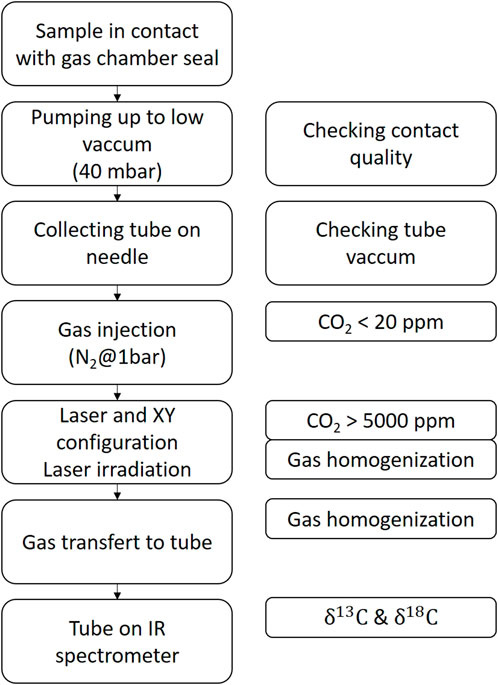
FIGURE 3. Step-by-step scheme of laser calcination gas collection protocol.

3 Metrological approach

Using the definitions given by the 2012 International Vocabulary of Metrology (JCGM 200:2012), the objective was to determine the statistical characteristics of the measuring device, such as measurement range, resolution, sensitivity, accuracy, fidelity, repeatability, and reproducibility. Thus, three methods—i) intercalibration, ii) ANOVA, and iii) GUM—were used in the following to determine the uncertainties associated with each statistical characteristic. The values for the measuring range, resolution, and sensitivity are tied to the characteristic of the optical spectrometer—notably the CO₂ concertation—within a range of 150 and 1,500 ppm. Intercalibration gave the accuracy of the transfer functions, the GUM method scaled accuracy and uncertainties, and the ANOVA gauge R&R study measured the repeatability and reproducibility of the method. The combination of these statistical approaches allows assessment of the validity of the laser preparation method and gives the maximum uncertainty related to the entire measurement process.

3.1 The GUM method

The method used to assess the accuracy and, therefore, the uncertainties of the measurements is the GUM method (ISO/IEC Guide 98-3:2008, acronym for “Guide to the expression of Uncertainly in Measurement”, 2008). This method is based on a first-order approximation of the uncertainties with the main assumption that the probability error is a random variable, i.e., the measurement error corresponds to the sum of the random errors and the systematic errors. The other key assumption is that measurement and probability errors are independent of each other. This method makes it possible to obtain a measurement uncertainty that combines both type-A (statistic, ${\sigma }_{\mathrm{A},\text{statistic}}$) and type-B (probabilistic) uncertainties. Systematic errors (type-B uncertainties) arise from the inhomogeneity of the material (${\sigma }_{\mathrm{B},\text{homogeneity}}$), the method of preparation (${\sigma }_{\mathrm{B},\text{preparation}}$), the method of analysis (${\sigma }_{\mathrm{B},\text{optical}\text{analysis}}$), and the transfer function (${\sigma }_{\mathrm{B},\text{transfer}\text{function}}$). The sources of systematic error were considered independent of each other. For the preparation and the analysis methods, the uncertainties associated with the systematic errors were retrieved from the manufacturers’ technical data sheets. However, as the inhomogeneity of the material is an unknown parameter, the associated uncertainty was also unknown. One hypothesis is then to consider this error as random and therefore part of the statistical uncertainty. Equation 1 summarizes all the uncertainties considered during the course of this study (1σ).

$\begin{array}{ll}\hfill {\sigma }_{\text{measure}}& =\sqrt{{{\sigma }_{\mathrm{A},\text{measure}}}^2+{{\sigma }_{\mathrm{B},\text{measure}}}^2}=\sqrt{{{\sigma }_{\mathrm{A},\text{statistic}}}^2+{{\sigma }_{\mathrm{B},\text{homogeneity}}}^2{+{\sigma }_{A,\text{preparation}}}^2+{{\sigma }_{\mathrm{B},\text{transfer}\text{function}}}^2+{{\sigma }_{\mathrm{B},\text{optical}\text{analysis}}}^2}\hfill \\ \hfill & \approx \sqrt{{{\sigma }_{\mathrm{A},\text{statistic}-\text{homogeneity}}}^2{+{\sigma }_{A,\text{preparation}}}^2+{{\sigma }_{\mathrm{B},\text{transfer}\text{function}}}^2+{{\sigma }_{\mathrm{B},\text{optical}\text{analysis}}}^2}\hfill \end{array}(1)$

3.2 Intercalibration

Intercalibration compares the method of analysis by laser calcination (laser technique) with the acid technique to determine if there is a transfer function, and the accuracy of the measurements obtained ${\sigma }_{\mathrm{B},\text{transfer}\text{function}}$. The objective was therefore to verify the robustness of the method from samples selected over a wide range of isotopic compositions. The intercalibration also aimed to scale the influence of the experimental parameters of the laser technique with the experimental values obtained and assess possible experimental isotopic fractionations. The latter was indeed expected in the case of oxygen isotope analysis because only two-thirds of the oxygen atoms in carbonate were converted into CO₂ molecules during the calcination reaction.

3.3 ANOVA gauge R&R study

To evaluate the uncertainty associated with the repeatability and reproducibility of the measurement method (from the sample to the optical spectroscopic analysis), an ANOVA (ANalysis Of VAriance) gauge R&R study was conducted on the complete process (Mandel, 1972; Tsa, 1988; Pan, 2004; Pan, 2006).

An adaptation of the ANOVA method was used here to identify the sources of variations by considering the inhomogeneity of the sample. These sources of variation are i) the area of analysis, ii) the operators, iii) the temporal stability of the analyses, and iv) the methods of analysis. Thus, considering these different parameters, the isotopic ratios must group according to i) the origin of the samples from the same block of the same rock; ii) several operators analyzing the same samples at different times; iii) the analyses being of the same samples by the two methods. The intra- and inter-group variations were then calculated to determine i) repeatability, ii) reproducibility, iii) the interaction between the sample and the analytical method, and iv) the variability between the measurement methods (Burdick et al., 2005).

Therefore, to determine the uncertainty of the CO₂ extraction (${\sigma }_{\mathrm{B},\text{preparation}}$), we used the ANOVA method to compare the acid and laser preparation methods. Using the definition of Korol et al. (2015), the uncertainty associated with the preparation (Eq. 2) comprised the repeatability ((i) of the ANOVA method) and the variability between the preparation techniques ((iv) of the ANOVA method):

${\sigma }_{\mathrm{A},\mathrm{p}\mathrm{r}\mathrm{e}\mathrm{p}\mathrm{a}\mathrm{r}\mathrm{a}\mathrm{t}\mathrm{i}\mathrm{o}\mathrm{n}}=\sqrt{{{\sigma }_{A,\text{repeatability}\text{preparation}\text{method}}}^2+{{\sigma }_{A,\text{variability}\text{of}\text{preparation}\text{technique}}}^2}(2)$

Accordingly, the uncertainty of the measurement process regarding the repeatability and reproducibility of the ANOVA method, as well as the measurement, is described by Eq. 3:

${\sigma }_{\text{measurement}\text{process}}=\sqrt{{{\sigma }_{\text{measure}}}^2+{{\sigma }_{A,\text{repeatability}}}^2+{{\sigma }_{A,\text{reproducibility}}}^2}(3)$

4 Results: validation of the laser calcination preparation method for isotopic measurements

The isotopic ratios given below are those obtained from either optical or mass spectrometers. At this stage, the transfer function is unknown. This transfer function may vary with different carrier gases. Here, N₂ was chosen, and all the measurements were made with N₂ because this inert gas is easily available and at a lower cost than, for example, synthetic air.

4.1 Influences of the experimental conditions of the laser on the value measured with the optical spectrometer

4.1.1 Influence of the quantity of evolved CO₂ on the isotopic ratios

The laser calcination process produces a quantity of CO₂ which depends on three main parameters: i) the optical absorption and scattering coefficients of the sample, ii) the incident laser power and, therefore, the light intensity of the laser beam focused on the sample, and iii) the exposure time. The CO₂ produced was mixed with N₂ and was collected and transferred to the spectrometers via gas sample tubes. The process, from generation to transfer to spectrometers, is passive by equilibration between the gas line and the gas sample tube; only part of the gas initially produced was thus used for isotopic analysis. It was therefore necessary to determine the quantity of CO₂, and therefore, the mass of carbonate transformed to obtain an accurate measurement (i.e., sensitivity of the calcination method). The documentation of the optical spectrometer used in this study suggests measuring CO₂ in a range of 400–1,500 ppm at 1 bar. During laser preparation, the quantity of CO₂ produced and measured by the collection chamber sensor is, at atmospheric pressure, typically between 3,000 and 50,000 ppm, depending on the irradiation and laser scanning process. The highest CO₂ concentration can nevertheless be analyzed, thanks to an internal dilution function of the optical spectrometer. No measurements of the concentration were actually transferred into the gas sampling tube; therefore, in the following, the fidelity of the isotopic ratios is reported against the initial quantity of CO₂ produced. For this, the analyses were performed as points (a fixed laser shot). To increase the quantity of CO₂ produced, it was then sufficient to produce several successive points (after a translation of the laser spot), each corresponding to a single laser shot. The choice to always have the same pattern allowed the same process during the calcination reaction. The tests were performed with the SN26 sample, which gives homogeneous results with its statistical uncertainty (type A) at 1σ (δ¹³C = 9.16‰ ± 0.08‰) when measuring using sector field IRMS. The laser calcination conditions were established so that a measurement point corresponds approximately to 3,500 ± 300 ppm.

Figure 4 presents the results of the carbon and oxygen isotopic composition measurements as a function of the quantity of CO₂ produced (i.e., the number of laser shots). Two operating regimes corresponding to a CO₂ threshold value of 5,000 ppm were observed. Below 5,000 ppm, δ¹³C was 8.14‰ ± 0.07‰ (n = 5, 1σ), and above 5,000 ppm, over concentrations from 5,000 to 30,000 ppm, δ¹³C was 8.60‰ ± 0.20‰ (n = 33, 1σ). The significant difference with the measurements obtained below 5,000 ppm with the acid method (δ¹³C = 9.16‰ ± 0.08‰) shows that it is necessary to produce enough CO₂ with a sensitivity threshold of approximately 8 mg of CaCO₃. The 12C-enriched deviation of the measured value at a pressure below 5,000 ppm is likely due to the small contribution of air-CO₂ with a δ¹³C usually around −10‰ in the laboratory.

FIGURE 4

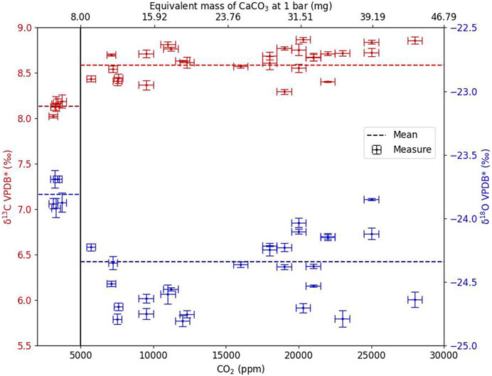
FIGURE 4. Carbon and oxygen isotopic composition measured on a Delta-Ray™ versus the quantity of CO₂ produced after laser calcination for the SN26 sample. VPDB* stands for isotopic compositions from optical spectrometer measurements before correction of potential laser calcination instrumental fractionation (i.e., transfer function).

In order to avoid isotopic variations induced by low CO₂ concentrations, and thus, to reduce the systematic errors of the analysis by optical spectroscopy, the CO₂ concentration produced after laser calcination was thereafter kept above the 5,000-ppm threshold.

An additional indicator was introduced to consider the effects of gas transfers between devices: the failure rate. This represents the number of measurements not giving the results of isotopic ratios (δ¹³C_carb and δ¹⁸O_carb) with the optical spectrometer that the spectrometer reported the measurement as not being carried out. This failure rate is defined by the number of failed measurements divided by the number of measurements taken per ≥5,000 ppm CO₂ samples. Figure 5 shows the variation of this indicator as a function of CO₂ concentration. For concentrations of at least 20,000 ppm, the failure rate becomes 0 and all the measurements are validated. The process is valid with a minimum of 5,000 ppm, but to ensure that all the measurements are correctly taken, the CO₂ concentration can be chosen higher than 20,000 ppm. The mass to be transformed of sample therefore corresponds to approximately 30 mg of CaCO₃. This failure rate was likely due to the many steps and mechanisms of collecting, transferring, and diluting gas between the collection chamber and the optical spectrometer.

FIGURE 5

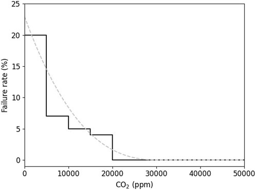
FIGURE 5. Optical spectrometer failure rate as a function of CO₂ concentration. The total number of measurements is 295, of which 30 are in the 0–5,000 ppm interval, 89 in the 5,000–10,000 ppm interval, 85 in the 10,000–15,000 ppm interval, 23 in the 15,000–20,000 ppm interval, 19 in the 20,000–25,000 ppm interval, 20 in the 25,000–30,000 ppm interval, 12 in the 30,000–35,000 ppm interval, 11 in the 40,000–45,000 ppm interval, and 6 in the 45,000–50,000 ppm interval.

The total number of measurements was 295, of which 30 are in the 0–5,000 ppm interval, 89 in the 5,000–10,000 ppm interval, 85 in the 10,000–15,000 ppm interval, 23 in the 15,000–20,000 ppm interval, 19 in the 20,000–25,000 ppm interval, 20 in the 25,000–30,000 ppm interval, 11 in the 30,000–35,000 ppm interval, 11 in the 40,000–45,000 ppm interval, and 6 in the 45,000–50,000 ppm interval.

4.1.2 Spatial resolution and areas of analysis

Reaching a concentration of at least 5,000 ppm of CO₂—at least 8 mg of converted CaCO₃—requires different protocols depending on the chemical nature of the sample and the geometry of the desired analysis volume. If the material is sufficiently absorbent, an integrated analysis over a depth of a few millimeters is possible (6 mm max—Figure 6B). In that case, the area analyzed roughly corresponds to an ablated spot of approximately 200–300 µm with a total HAZ (heat-affected zone) surface diameter between 0.3 and 1 mm (Figures 6A, B). If the material is not a priori homogeneous in depth but is on the surface, a surficial analysis can be performed, which changes from an orthogonal to a tangent direction of the laser beam in relation to the sample surface. The volume of transformed carbonate then appears in the form of a line of small width (roughly identical to the diameter of the laser spot, <500 µm) and of small depth (<1 mm). If the surface inhomogeneity is incompatible with a line length corresponding to the minimum quantity of CO₂, it is possible to split this line into several segments, juxtapose them, and then form a square or rectangular pixel composed of elementary lines with a maximum resolution of three lines/mm (Figure 6C).

FIGURE 6

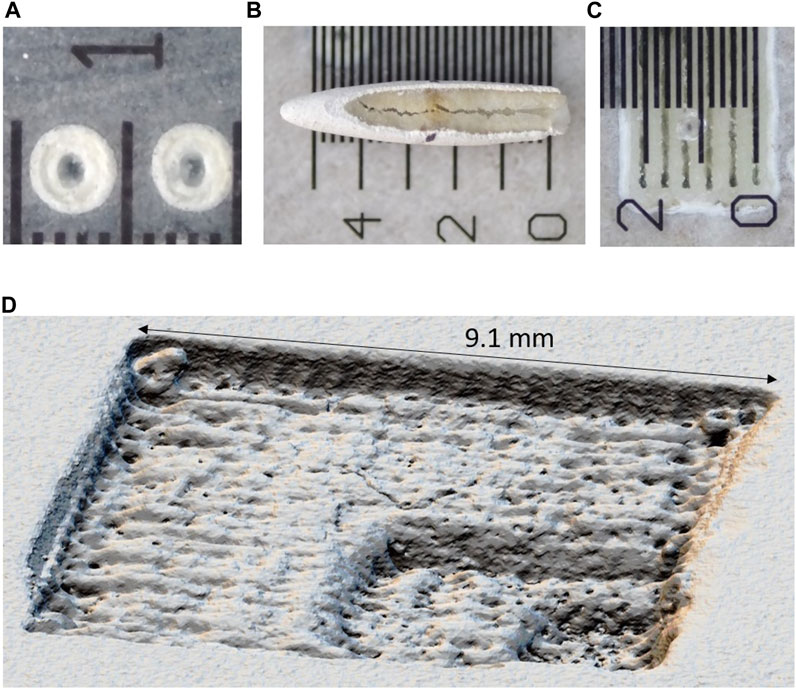
FIGURE 6. Example of areas of analysis: (A) single spot with a hole diameter of approximately 200–300 μm; (B) 3D visualization of HAZ (heat-affected zone) with extract of transformed material; (C) multiline mapping with a maximum resolution of 3 lines/mm; (D) example of stratigraphic analysis with tree layers transformed and removed by laser.

When the calcination process is well-controlled (depth and width of transformed material and size of the HAZ), it is also possible to conduct layer-by-layer (stratigraphic) and “tomographic” analyses. If the focal plane of the laser spot is fixed, this corresponds to about 3–4 depths of analysis before the laser beam diverges too much. If the focal plane can be moved vertically, it is possible to “dig” the material deeper. Figure 6D presents an example of “tomographic analysis” made with a fixed focal plane and for three different depths.

4.2 Evaluation of measurement uncertainties with this new method

The measurement process incorporates many possible sources of uncertainty that can alter the analytical performance of the laser calcination method. To be able to extract the total uncertainty, it is therefore necessary to evaluate each individual source of uncertainty and their combination (see Section 3).

4.2.1 Influence of the reference gas’ isotopic composition on the measurement’s uncertainty

The optical spectrometer used in this study measures the isotopic ratio of an unknown gas against the molecular ratio of a reference gas. In our case, the reference gas has the following certified isotopic composition and uncertainties: δ¹³C_VPDB=−25.5‰ ± 0.15‰ and δ¹⁸O_VPDB=−24.4‰ ± 0.15‰. Using the propagation of uncertainties, we evaluated how the fixed reference gas’ isotopic composition can affect the uncertainties associated with samples showing variable isotopic compositions between −30‰ and +30‰ (Figure 7). The uncertainty corresponding to a sample having a δ¹³C_carb of −30‰ is close to the reference gas uncertainty (0.15‰) as expected; however, for sample having a δ¹³C_carb distant to the reference gas value (+30‰), the uncertainty is 0.16‰. Variations in uncertainty of measured δ¹³C over this range are therefore 0.01‰. For oxygen, the uncertainty between −30‰ and +30‰ is also within 0.01‰. In both cases, as the variations in uncertainty over this range are negligible (less than 10% of the uncertainty from the reference gas specification), the uncertainty associated with using this single reference gas is a constant equal to 0.15‰ of the isotopic composition of carbon and oxygen.

FIGURE 7

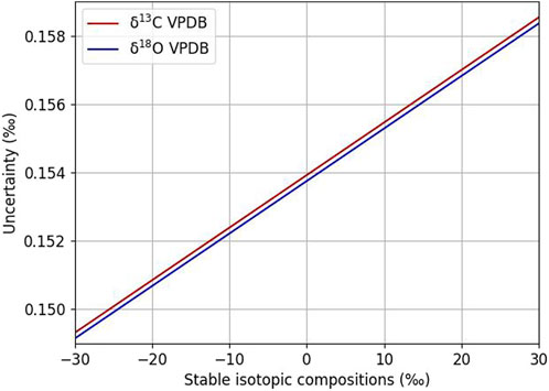
FIGURE 7. Evolution of the uncertainty associated with reference gas scaling over a range of measured isotopic compositions.

4.2.2 Uncertainty associated with optical spectrometer analysis

During the analysis, the final uncertainty was the sum of the repeatability, the precision of the optical spectrometer, and the reference gas uncertainty. The sum of uncertainty considering the reproducibility ($\left.{\sigma }_{\mathrm{C},\text{reproducibility}}=0.07‰,{\sigma }_{\mathrm{O},\text{reproducibility}}=0.10‰\right)$ and precision $\left({\sigma }_{\mathrm{C},\text{precision}}=0.15‰,{\sigma }_{\mathrm{O},\text{precision}}=0.20‰\right)$ given by the manufacturer is expressed below in Eq. 3 for carbon and oxygen isotopes:

$\left\{\begin{array}{c}{\sigma }_{\mathrm{C},\text{Delta}-\text{Ray}}=\sqrt{{{\sigma }_{\mathrm{C},\text{reproducibility}}}^2+{{\sigma }_{\mathrm{C},\text{precision}}}^2}=\sqrt{{0.07}^2+{0.15}^2}=0.17‰\\ {\sigma }_{\mathrm{O},\text{Delta}-\text{Ray}}=\sqrt{{{\sigma }_{\mathrm{O},\text{reproducibility}}}^2+{{\sigma }_{\mathrm{O},\text{precision}}}^2}=\sqrt{{0.10}^2+{0.20}^2}=0.23‰\end{array}\right.(4)$

We presume that the uncertainties of the reference gas (0.15‰ for carbon and oxygen—see Section 4.2.1) and of the optical spectrometer are independent. A numerical approach, based on Monte Carlo-type simulation (Oliveira, 2013), is used to combine the uncertainties linked to the reference gas with the uncertainties of the spectrometer.

To carry out this simulation, we use the definition of the isotopic ratio X (Eq. 5):

$\delta X_{\text{ech}/VPDB}=1000\bullet \left(\frac{R_{sample}}{R_{VPDB}}-1\right),(5)$

where X corresponds to ¹³C or ¹⁸O, R is the molecular ratio of ¹³C/¹²C or ¹⁸O/¹⁶O, and sample corresponds to the unknown gas measured by the spectrometer and VPDB to the reference gas. In fact, the optical spectrometer transforms Eq. 5 to a one-parameter equation named $R_{corrsample}$, which is a correction of the value of the molecular ratio by the molecular ratio of the reference gas:

$\left\{\begin{array}{c}{\delta }^{13}{C}_{ech/VPDB}=89444\bullet R_{corrsample}-1000,\\ {\delta }^{18}{O}_{ech/VPDB}=239420\cdot R_{corrsample}-1000.\end{array}\right.(6)$

In order to consider the effect of having a single reference gas and the metrological performance of the optical spectrometer, we assume that the uncertainty associated with the reference gas affects the slope named a (equal to 89444 for carbon and 239420 for oxygen) and the uncertainty of the optical spectrometer modifies $R_{corrsample}$.

In the simulation, we fixed the starting values at the isotopic values of the reference gas (i.e., −25.5‰ for carbon and −24.4‰ for oxygen), and we consider that the uncertainties are constant over a range of carbon and oxygen isotopes between −30.0‰ and +30.0‰ (see paragraph in Section 4.2.1). The corrected molecular ratio ($R_{corrsample}$) corresponding to this starting value is named Rstart.

Using the propagation of uncertainties, we obtain an uncertainty on the slope named $\partial$ a and $R_{corrsample}$ named $\partial R_{corrsample}$—respectively equal to 14 and 1.90 $·$ 10-6 for carbon and 37 and 8.35 $·$ 10-7 for oxygen.

The Monte Carlo simulation is then run with randomly chosen Rsimulated sample and slope in the following intervals: $\left[R_{start}-2\cdot \partial R_{corrsample},R_{start}+2\cdot \partial R_{corrsample}\right]$ and $\left[a-2\cdot \partial a,a+2\cdot \partial a\right]$ before isotopic composition recalculation. By repeating these operations one million times (corresponding to a numerical error of 0.01%), the average obtained then equals the value of the reference gas, and the standard deviation corresponds to the uncertainty associated with the optical analysis (Figure 8).

FIGURE 8

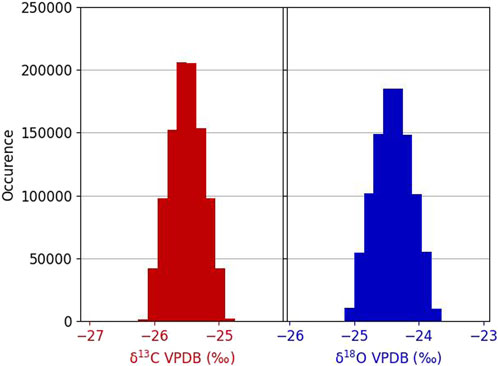
FIGURE 8. Distribution histograms of carbon and oxygen isotope compositions after Monte Carlo simulation of repeated optical spectrometer analysis of a fixed isotopic ratio.

Figure 8 presents the histograms obtained after the Monte Carlo simulation. The average obtained is, as expected, equal to that of the reference gas. The combined standard deviation is equal to 0.26‰ for carbon and 0.29‰ for oxygen (Eq. 7):

$\left\{\begin{array}{c}{\sigma }_{\mathrm{C},\mathrm{B}-\text{optical}\text{analysis}}=0.26‰,\\ {\sigma }_{\mathrm{O},\mathrm{B}-\text{optical}\text{analysis}}=0.29‰.\end{array}\right.(7)$

4.2.3 Carbon and oxygen stable isotope composition intercalibrations

A critical step in validating the laser calcination technique as a metrological method is determining the transfer functions of the isotopic ratios between the laser calcination and the acid techniques. Table 2 summarizes the isotopic measurements performed during this study.

TABLE 2

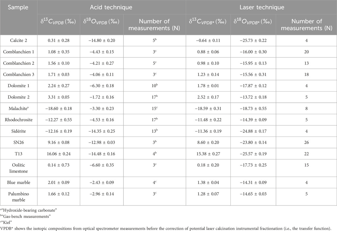
TABLE 2. Stable isotopic compositions of carbon and oxygen measured after the classical “acid technique” and “laser technique.”

The uncertainties reported in Table 2 and displayed on the intercalibration curves in Figure 9 are the statistical uncertainties resulting from N repeated measurements per sample; they are given at 1σ and reflect the external reproducibility.

FIGURE 9

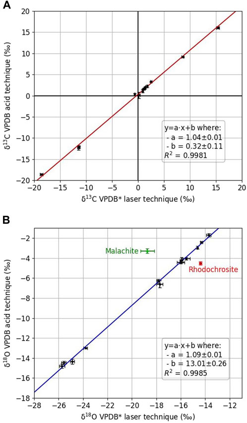
FIGURE 9. Intercalibration plots of carbon (A) and oxygen (B) isotopic compositions of natural samples between acid-IRMS and laser calcination–optical laser spectroscopy (regression lines correspond to linear adjustments of individual mean values). VPDB* stands for isotopic compositions from optical spectrometer measurements before correction of potential laser calcination instrumental fractionation (i.e., transfer function).

The linear adjustments for carbon and oxygen (Eq. 8) are

$\begin{array}{c}{\mathrm{\delta }}^{13}{C}_{VPDB}\left(″{\text{acid}}^{″}\text{\hspace{0.17em}IRMS\hspace{0.17em}}\right)=1.04\bullet {\mathrm{\delta }}^{13}{C}_{VPDB}*\left(\text{Laser}-\text{Laser\hspace{0.17em}}\right)+0.32\\ {\mathrm{\delta }}^{18}{O}_{VPDB}\left(″{\text{acid}}^{″}\text{\hspace{0.17em}IRMS}\right)=1.09\bullet {\mathrm{\delta }}^{18}{O}_{VPDB}*\left(\text{Laser}-\text{Laser\hspace{0.17em}}\right)+13.01\end{array}(8)$

and are associated with correlation coefficients better than 0.998.

Malachite and rhodochrosite were excluded from the linear regression for oxygen isotopes. The deviation of these two carbonates from the overall observed correlation may arise from the fact that malachite contained hydroxide in its crystalline lattice. Other matrix effects, probably due to the nature of the cations (e.g., Mn in rhodochrosite) in the analyzed carbonates, or to complex mixed mineralogy, may also add instrumental fractionation during calcination yet to be fully determined.

4.2.4 Uncertainty associated with the transfer function

4.2.4.1 Linear regression

In order to determine an uncertainty for the coefficients of the linear regression, we presume that the assumption of residual normality—a normal distribution—applies only to the error of the relationship between the measured and the predicted value calculated using the linear regression.

For the carbon isotopic composition, the uncertainty (1σ) estimated under the assumption of residual normality is 0.11‰ (intercept) and 0.01‰ (slope). As the intercept is close to 0 and the slope close to 1, the VPDB* values given by this new method of preparation are close to the values obtained by the traditional method (and probably at least partly reflect the inhomogeneity of the samples), and correction factors are minor. For the oxygen isotopic composition, the uncertainty (1σ), estimated under the assumption of residual normality, is 0.26‰ (intercept) and 0.01‰ (slope). However, because the intercept is around +13‰ (Figure 9), an instrumental isotopic fractionation during laser calcination is evidenced. This fractionation seems constant and can be easily corrected by adding a factor of +13.01‰ to the VPDB* measurements, given that the slope of the regression line is close to unity.

4.2.4.2 Monte Carlo simulation with measurement uncertainties

In order to evaluate the statistical uncertainties arising from the intercalibration (VPDB* to VPDB), a Monte Carlo simulation was conducted (Oliveira, 2013). The principle of this simulation is to choose the values of the measurements uniformly and randomly within the uncertainty of the statistical measurements (type A) with an error risk of 5%—twice the static uncertainty. By repeating this step one million times (making possible a numerical error of the order of a hundredth of a percent), the mean and the standard deviation of the simulated slope and intercept coefficients give in Eq. 9 the values of intercalibration with associated uncertainty.

$\begin{array}{c}{\mathrm{\delta }}^{13}{C}_{VPDB}\left(″{\text{acid}}^{″}\text{\hspace{0.17em}IRMS\hspace{0.17em}}\right)=\left(1.04\pm 0.01\right)\bullet {\mathrm{\delta }}^{13}{C}_{VPDB}*\left(\text{Laser}-\text{Laser\hspace{0.17em}}\right)+\left(0.31\pm 0.11\right)\\ {\mathrm{\delta }}^{18}{O}_{VPDB}\left(″{\text{acid}}^{″}\text{\hspace{0.17em}IRMS}\right)=\left(1.09\pm 0.02\right)\bullet {\mathrm{\delta }}^{18}{O}_{VPDB}*\left(\text{Laser}-\text{Laser\hspace{0.17em}}\right)+\left(13.01\pm 0.38\right)\end{array}(9)$

Compared with the raw linear regression uncertainties (paragraph in Section 4.2.4.1), the simulated uncertainties have increased for oxygen and remained the same for carbon. For carbon and oxygen, the intercept at the origin and slope varied up to 3%, which we consider negligible. Finally, given the Monte Carlo simulation results, we define the uncertainties of the transfer function as primarily controlled by the uncertainties on the intercept thus (Eq. 10):

$\left\{\begin{array}{c}{\sigma }_{\mathrm{C},\mathrm{B}-\text{transfert}\text{function}}=0.11‰\\ {\sigma }_{\mathrm{O},\mathrm{B}-\text{transfert}\text{function}}=0.38‰.\end{array}\right.(10)$

4.2.5 Evaluation of measurement uncertainty associated with the CO₂ preparation method

In order to assess the uncertainty of the laser preparation (Eq. 2), an ANOVA method was applied by comparing the gas preparation methods (laser calcination, acid wet chemistry) of six series (three by laser calcination and three by acid preparation) of five measurements for three samples of Comblanchien limestone. Once the gas was extracted, it was analyzed for both methods by optical spectroscopy.

With this method, the uncertainty associated with repeatability (according to an interpretation of JCGM 200:2012, repeatability is the measurement precision after repeated measurements of the same sample in the same analytical conditions) and variability between preparation methods (the variability between preparation methods determines the systematic error between these two measurement methods) is determined by Eq. 11:

$\left\{\begin{array}{c}{\sigma }_{\mathrm{A},\text{preparation},\mathrm{C}}=\sqrt{{{\sigma }_{A,\text{repeatability}\text{preparation}\text{method}}}^2+{{\sigma }_{A,\text{variability}\text{of}\text{preparation}\text{technique}}}^2}=0.02‰\\ {\sigma }_{\mathrm{A},\text{preparation},\mathrm{O}}=\sqrt{{{\sigma }_{A,\text{repeatability}\text{preparation}\text{method}}}^2+{{\sigma }_{A,\text{variability}\text{of}\text{preparation}\text{technique}}}^2}=0.02‰.\end{array}\right.(11)$

The final uncertainty on the isotopic measure given at 1σ is as follows (Eq. 12):

$\left\{\begin{array}{c}{\sigma }_{\text{measure},\mathrm{C}}=\sqrt{{{{{{{\sigma }_{A,\text{preparation}}}^2+\sigma }_{\mathrm{B},\text{transfert\hspace{0.17em}function}}}^2+\sigma }_{\mathrm{B},\text{optical\hspace{0.17em}analysis}}}^2}=0.28‰\\ {\sigma }_{\text{measure},\mathrm{O}}=\sqrt{{{\sigma }_{A,\text{preparation}}}^2+{{{\sigma }_{\mathrm{B},\text{fonction}\text{de}\text{transfert}}}^2+{\sigma }_{\mathrm{B},\text{optical}\text{analysis}}}^2}=0.48‰.\end{array}\right.(12)$

4.2.6 Evaluation of the repeatability and reproducibility of the measurement process uncertainties using the laser calcination laser–laser method

When all uncertainties are considered, the uncertainty of the measurement process is given in Eq. 13 (combining Eqs 1, 2).

$\begin{array}{ll}\hfill {\sigma }_{\text{measurement}\text{process}}& =\sqrt{{{\sigma }_{A,\text{preparation}}}^2+{{\sigma }_{\mathrm{B},\text{transfer}\text{function}}}^2+{{\sigma }_{\mathrm{B},\text{optical}\text{analysis}}}^2+{{\sigma }_{A,\text{repeatability}}}^2+{{\sigma }_{A,\text{reproducibility}}}^2}\hfill \\ \hfill & =\sqrt{{{\sigma }_{measure}}^2+{{\sigma }_{A,\text{repeatability}}}^2+{{\sigma }_{A,\text{reproducibility}}}^2}.\hfill \end{array}(13)$

The measurement process uncertainties correspond to the repeatability, reproducibility, and uncertainty associated with CO₂ production by laser calcination, and uncertainty associated with the optical analysis and the transfer function.

To evaluate ${\sigma }_{\text{repeatability}}$ and ${\sigma }_{\text{reproducibility}}$, ANOVA was performed on the isotopic results given by five homogeneous samples of Comblanchien analyzed at five different times of a year and by four different operators. The results of the various uncertainties given at 1σ are shown in Table 3.

TABLE 3

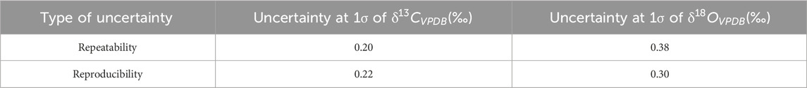
TABLE 3. Result of ANOVA analysis. According to an interpretation of JCGM 200:2012, repeatability is the measurement precision after repeated measurements of the same sample in the same analytical conditions, and reproducibility is the measurement precision after repeated measurements of the same sample in the same analytical conditions but by different operators.

The uncertainty associated with carbon is finally mostly reflected by the gas analysis uncertainty (i.e., order 0 of a limited development applied to the measurement process terms), which means that this method of preparation by laser calcination is robust. For oxygen, the final uncertainty is mostly reflected by the transfer function, meaning that a local calibration of the sample to be analyzed needs to be performed using standards.

The uncertainty associated with the measurement process is as follows in Eq. 14:

$\left\{\begin{array}{c}{\sigma }_{\text{measurement}\text{process},\mathrm{C}}=\sqrt{{{\sigma }_{\text{Bmeasure},\mathrm{C}}}^2+{{\sigma }_{\mathrm{A},\text{repeatability},\mathrm{C}}}^2+{{\sigma }_{\mathrm{A},\text{reproducibility},\mathrm{C}}}^2}=0.41‰\\ {\sigma }_{\text{measurement}\text{process},\mathrm{O}}=\sqrt{{{\sigma }_{\text{measure},\mathrm{O}}}^2+{{\sigma }_{\mathrm{A},\text{repeatability},\mathrm{O}}}^2+{{\sigma }_{\mathrm{A},\text{reproducibility},\mathrm{O}}}^2}=0.68‰\end{array}\right.(14)$

The GUM method recommends, for confidence in observing variations in isotopic composition on a sample, giving the uncertainty at 5.15σ, which corresponds here to Eq. 15

$\left\{\begin{array}{c}{\sigma }_{\text{measurement}\text{process},\mathrm{C},\text{GUM}}=2.11‰\\ {\sigma }_{\text{measurement}\text{process},\mathrm{O},\text{GUM}}=3.51‰.\end{array}\right.(15)$

In a general case, it is necessary to give at least the uncertainties at 3σ, which correspond to 99.7% of the values in the case where the distribution of the measurements follows a normal law. In this case, the uncertainty of the isotopic ratio associated with carbon is 1.23‰ and 2.04‰ for oxygen.

5 Example of spatially resolved laser–laser isotopic measurements

The sample used to exemplify spatially resolved chemostratigraphic application was a travertine limestone from a hot spring site at the Mount Rinjani volcano (Lombok Island, Indonesia, −8.3898948 S, 116.4204031 E). Its stratigraphy showed parallel, millimetric, white, and brown alternation extending over the depth of the sample. Nineteen lines of laser calcination (Figure 10) were performed along its stratigraphy on specific layers based on their color contrasts. Calcination line 18, made on the bottom blackish part (mixed silicate–carbonate) of the sample, was not measured for its isotopic compositions by the optical spectrometer due to poor reaction yield.

FIGURE 10

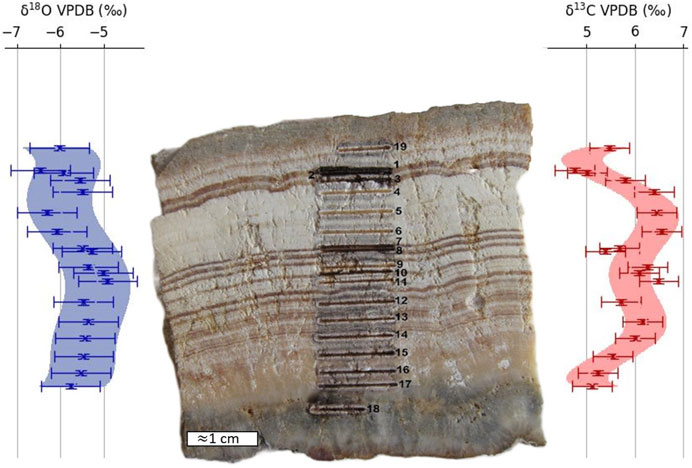
FIGURE 10. Chemostratigraphic variations in oxygen and carbon isotopic compositions measured on a hot spring travertine sample. Polynomial interpolation of degree 6 is shown. The uncertainties are those defined at 1σ of the measurement process.

Figure 10 presents the chemostratigraphic variations in oxygen and carbon isotopic composition corresponding to the calcination lines. For oxygen, the measured variations are of the same magnitude as the uncertainty of the measurement process. The values of the different calcination lines are thus statistically identical. Conversely, for carbon, the sample shows variations greater than the measurement uncertainty. The strongest variations are located between calcination lines 1 and 7, with δ¹³C_VPDB values ranging from 4.8‰ to 6.5‰. The interpretation of these isotopic changes is beyond the scope of this paper; nevertheless, a decrease in evaporation regime and/or an increasing contribution of carbon from ¹²C-enriched volcanic or organic source may account for the observed fewer ¹³C enriched values in calcination lines 7 to 3.

6 Conclusion and future directions

This study presents the development of a transportable laser carbonate preparation method. In order to justify the performance of this new device and method of carbonate preparation by laser ablation, a dedicated measurement protocol was designed and tested on a paired isotopic ratio optical mass spectrometer. A metrological study was conducted, showing that the uncertainty associated with the sample’s measurements after intercalibration are 0.41‰ and 0.68‰ for carbon and oxygen isotopes, respectively. The uncertainty associated with the carbon isotope is less than oxygen, and a linear correction function is needed for oxygen isotopes to be properly scaled to VPDB scale assessed by the acid digestion IRMS. The metrological work allows evaluation of the uncertainty associated with the laser carbonate preparation method, which is of the same magnitude as the acid digestion preparation method. Finally, the carbonate preparation system was used for detailed spatially resolved chemostratigraphic isotopic measurements of a layered travertine limestone at reduced cost and time, exclusively using a compact bench-top device. Such new, fast, spatially resolved, and transportable isotopic systems will allow novel on-site or field applications and will greatly facilitate future work on small scale isotopic variability of natural carbonate samples such as along shells growth increments. Furthermore, laser spectroscopy has recently been used to measure the clumped isotopic composition of carbon dioxide (e.g., Prokhorov et al., 2019; Wang et al., 2019). When combined with carbonate laser calcination, such laser technology may provide a quick and simple method of measuring rare and doubly substituted CO₂ isotopologs of carbonates.

Data availability statement

The original contributions presented in the study are included in the article/Supplementary Material; further inquiries can be directed to the corresponding author.

Author contributions

AP: Conceptualization, Data curation, Formal Analysis, Investigation, Methodology, Software, Writing–original draft, Writing–review and editing. CT: Conceptualization, Funding acquisition, Investigation, Methodology, Supervision, Writing–original draft, Writing–review and editing. OM: Conceptualization, Funding acquisition, Investigation, Methodology, Supervision, Writing–original draft, Writing–review and editing. IJ: Formal Analysis, Investigation, Methodology, Supervision, Writing–review and editing. PS: Conceptualization, Resources, Writing–review and editing. KK: Resources, Writing–review and editing.

Funding

The author(s) declare financial support was received for the research, authorship, and/or publication of this article. This work is a contribution to the “Investissements SATT SAYENS” project ISOLASER and was also supported by the FEDER Bourgogne Franche-Comté.

Acknowledgments

The authors thank the GISMO platform and its staff (Biogéosciences, Université de Bourgogne, UMR CNRS 6282, France). Jerome Thomas is warmly acknowledged for providing access to the Dijon Museum collection of minerals. Brice Gourier and Julien Lopez from the CRM (Centre Ressource Mécanique) of ICB are acknowledged for their help in building the calcination system. We thank Michael Roden for handling this manuscript and two anonymous referees for constructive comments.

Conflict of interest

The authors declare that the research was conducted in the absence of any commercial or financial relationships that could be construed as a potential conflict of interest.

Publisher’s note

All claims expressed in this article are solely those of the authors and do not necessarily represent those of their affiliated organizations, or those of the publisher, the editors, and the reviewers. Any product that may be evaluated in this article, or claim that may be made by its manufacturer, is not guaranteed or endorsed by the publisher.

References

Burdick, R. K., Park, Y.-J., Montgomery, D., and Borror, C. M. (2005). Confidence intervals for misclassification rates in a gauge R&R study. J. Qual. Technol. 37 (4), 294–303. doi:10.1080/00224065.2005.11980332

CrossRef Full Text | Google Scholar

Fischer, T., and Lopez, T. (2016). First airborne samples of a volcanic plume for δ¹³C of CO₂ determinations. Geophys. Res. Lett. 43 (7), 3272–3279. doi:10.1002/2016GL068499

CrossRef Full Text | Google Scholar

Garcia-Anton, E., Cuezva, S., Fernandez-Cortes, A., Benavente, D., and Sanchez-Moral, S. (2014). Main drivers of diffusive and advective processes of CO₂-gas exchange between a shallow vadose zone and the atmosphere. Int. J. Greenh. Gas Control 21, 113–129. doi:10.1016/j.ijggc.2013.12.006

CrossRef Full Text | Google Scholar

Korol, W., Bielecka, G., Rubaj, J., and Walczyński, S. (2015). Uncertainty from sample preparation in the laboratory on the example of various feeds. Accreditation Qual. Assur. 20, 61–66. doi:10.1007/s00769-014-1096-x

CrossRef Full Text | Google Scholar

Mandel, J. (1972). Repeatability and reproducibility. J. Qual. Technol. 4 (2), 74–85. doi:10.1080/00224065.1972.11980520

CrossRef Full Text | Google Scholar

McCrea, J. (1950). On the isotopic chemistry of carbonates and a paleotemperature scale. J. Chem. Phys. 18 (6), 849–857. doi:10.1063/1.1747785

CrossRef Full Text | Google Scholar

Oliveira, P. R. (2013). Theory and applications of Monte Carlo simulations (Norderstedt: BoD–Books on Demand).

Google Scholar

Pan, J.-N. (2004). Determination of the optimal allocation of parameters for gauge repeatability and reproducibility study. Int. J. Qual. Reliab. Manag. 21 (6), 672–682. doi:10.1108/02656710410542061

CrossRef Full Text | Google Scholar

Pan, J.-N. (2006). Evaluating the gauge repeatability and reproducibility for different industries. Berlin, Germany: Springer, 499–518.

CrossRef Full Text | Google Scholar

Prokhorov, I., Kluge, T., and Janssen, C. (2019). Laser absorption spectroscopy of rare and doubly substituted carbon dioxide isotopologues. Anal. Chem. 91 (24), 15491–15499. doi:10.1021/acs.analchem.9b03316

PubMed Abstract | CrossRef Full Text | Google Scholar

Rizzo, A., Jost, H.-J., Caracausi, A., Paonita, A., Liotta, M., and Martelli, M. (2014). Real-time measurements of the concentration and isotope composition of atmospheric and volcanic CO₂ at Mount Etna (Italy). Geophys. Res. Lett. 41 (7), 2382–2389. doi:10.1002/2014GL059722

CrossRef Full Text | Google Scholar

Śliwiński, M. G., Kitajima, K., Kozdon, R., Spicuzza, M. J., Denny, A., and Valley, J. W. (2017). In situ δ¹³C and δ¹⁸O microanalysis by SIMS: a method for characterizing the carbonate components of natural and engineered CO₂-reservoirs. Int. J. Greenh. Gas Control 57, 116–133. doi:10.1016/j.ijggc.2016.12.013

CrossRef Full Text | Google Scholar

Thomazo, C., Sansjofre, P., Musset, O., Cocquerez, T., and Lalonde, S. (2021). In situ carbon and oxygen isotopes measurements in carbonates by fiber coupled laser diode-induced calcination: a step towards field isotopic characterization. Chem. Geol. 578, 120323. doi:10.1016/j.chemgeo.2021.120323

CrossRef Full Text | Google Scholar

Tsai, P. (1988). Variable gauge repeatability and reproducibility. Qual. Eng. 1 (1), 107–115. doi:10.1080/08982118808962642

CrossRef Full Text | Google Scholar

Valley, J. W., Kita, N. T., and Fayek, M. (2009). In situ oxygen isotope geochemistry by ion microprobe. MAC short course Second. ion mass Spectrom. earth Sci. 41, 19–63.

Google Scholar

Wang, Z., Nelson, D. D., Dettman, D. L., McManus, J. B., Quade, J., Huntington, K. W., et al. (2019). Rapid and precise analysis of carbon dioxide clumped isotopic composition by tunable infrared laser differential spectroscopy. Anal. Chem. 92 (2), 2034–2042. doi:10.1021/acs.analchem.9b04466

CrossRef Full Text | Google Scholar