 Haipeng Yu
 Rohan L. Fernando
 Jack C. M. Dekkers
- 1Department of Animal Sciences, University of Florida, Gainesville, FL, United States
- 2Department of Animal Science, Iowa State University, Ames, IA, United States
Background: To address the limitations of commonly used cross-validation methods, the linear regression method (LR) was proposed to estimate population accuracy of predictions based on the implicit assumption that the fitted model is correct. This method also provides two statistics to determine the adequacy of the fitted model. The validity and behavior of the LR method have been provided and studied for linear predictions but not for nonlinear predictions. The objectives of this study were to 1) provide a mathematical proof for the validity of the LR method when predictions are based on conditional means, regardless of whether the predictions are linear or non-linear 2) investigate the ability of the LR method to detect whether the fitted model is adequate or inadequate, and 3) provide guidelines on how to appropriately partition the data into training and validation such that the LR method can identify an inadequate model.
Results: We present a mathematical proof for the validity of the LR method to estimate population accuracy and to determine whether the fitted model is adequate or inadequate when the predictor is the conditional mean, which may be a non-linear function of the phenotype. Using three partitioning scenarios of simulated data, we show that the one of the LR statistics can detect an inadequate model only when the data are partitioned such that the values of relevant predictor variables differ between the training and validation sets. In contrast, we observed that the other LR statistic was able to detect an inadequate model for all three scenarios.
Conclusion: The LR method has been proposed to address some limitations of the traditional approach of cross-validation in genetic evaluation. In this paper, we showed that the LR method is valid when the model is adequate and the conditional mean is the predictor, even when it is a non-linear function of the phenotype. We found one of the two LR statistics is superior because it was able to detect an inadequate model for all three partitioning scenarios (i.e., between animals, by age within animals, and between animals and by age) that were studied.
Introduction
Advances in high-throughput genotyping have enabled the implementation of genomic prediction, which has facilitated the genetic improvement of animals and plants based on more accurate estimated breeding values (EBV) at an early age (e.g., Meuwissen et al., 2001; Dekkers and Hospital, 2002; Bernardo and Yu, 2007; Habier et al., 2011; Wolc et al., 2011; Morota et al., 2013). Various genomic prediction models have been proposed and prediction performance across or within models is usually evaluated by cross-validation (CV) methods (Utz et al., 2000; Meuwissen et al., 2001; Saatchi et al., 2011; Morota and Gianola, 2014). With CV, the data set is partitioned into training and validation sets, with the training set used to fit a prediction model and estimate the breeding values (BV) of individuals in the validation set. Prediction performance is commonly evaluated with the statistic of predictivity, which is the correlation coefficient between the EBV and phenotypes adjusted for fixed effects of individuals in the validation set. Scaling predictivity by the square root of heritability (h2) provides an estimator for prediction accuracy of the EBV (Legarra et al., 2008; Serão et al., 2016), defined as the correlation between true and estimated breeding values. While accuracy estimated with CV has been widely used to quantify the performance of genomic prediction models, pre-correcting phenotypes in the validation set using estimates of fixed effects obtained using the whole data set will overestimate the accuracy when multiple levels of fixed effects are present (Legarra and Reverter, 2018). Additional limitations include that it cannot be applied to complex models (e.g., models with random regression, sex limited traits, maternal effects, additive and non-additive effects), indirect traits (e.g., unobserved latent traits), and traits with low h2 (Legarra and Reverter, 2018).
To address these limitations of the CV methodology, Legarra and Reverter (2018) proposed a linear regression (LR) method to estimate the accuracy of genomic prediction implicitly assuming the fitted model is correct. The LR method quantifies the population accuracy of predictions based on the correlation between EBV of individuals in the validation set estimated using the training set and the EBV of those same individuals estimated using the combined training and validation sets. In the LR method literature, the training set is referred to as the partial data set (p) and the combined training and validation data set is referred to as the whole data set (w). The LR estimator of population accuracy is theoretically justified only when the fitted model is adequate. Thus the LR method also provides two statistics that can be used to check if the model is adequate.
The LR method was mathematically justified by Legarra and Reverter (2018) based on results from Reverter et al. (1994). Macedo et al. (2020) investigated the behavior and properties of the LR method by analyzing simulated data with pedigree-based genetic models. They studied the LR estimators of population bias and accuracy of predictions by using wrong values of h2 in the analysis and by fitting wrong models that ignored the environmental trend through the simulated generations, and claimed that “the LR method works reasonably well for detection of bias when the model used is robust or close to the true model, and that it works well for estimation of accuracy even when the model is not good.” Validity and performance of the LR method for a non-linear model was explored by Bermann et al. (2021). In their study, they evaluated the performance of the LR method by fitting a threshold model to simulated data and also applied it to real data to estimate the increase in accuracy by adding genomic information. Based on the results from the simulated data, they concluded that the LR method can be useful to estimate the directions of bias, dispersion, and accuracy, though the LR estimators had different magnitudes compared to the true estimators. The original proof of the LR method (Legarra and Reverter, 2018) was based on the setting where the whole data set had additional phenotype records relative to the partial data set. Belay et al. (2022) recently showed that the LR method can also be applied to the setting where the whole data set has additional genotypes (rather than phenotypes) relative to the partial data set. They used the LR method to evaluate the bias and accuracy in single-step genomic predictions.
While the validity and performance of LR method has been explored using linear and non-linear models in previous studies (Macedo et al., 2020; Bermann et al., 2021), a mathematical proof of its validity for non-linear methods of prediction has not yet been presented. In addition, studies about the performance of the LR method when a model other than the true model is fitted are still relatively scarce in the literature. The objectives of this study were to 1) present a mathematical proof of the validity of the LR method when predictions are based on the conditional mean, regardless of whether it is a linear or non-linear function of the data 2) investigate the ability of the LR method to detect whether the fitted model is adequate or inadequate, and 3) provide guidelines on how to partition the data set such that the LR method can detect the use of an inadequate model.
Theory
Notation
In the LR method, Legarra and Reverter (2018) used var(x) to denote the variance of a random element, x, sampled from a single realization of the random vector x, and Var(x) to denote the variance-covariance matrix for the vector x. Similarly, they used cov(x, y) to denote the covariance between randomly sampled xi and yi and Cov(x, y) to denote the covariance matrix between the vectors x and y. Let u denote the vector of BV of the validation animals, and
Proof of the validity of the LR method when the conditional mean is used for prediction
Legarra and Reverter (2018) developed the LR method for best linear unbiased prediction (BLUP) by showing that
It is well known that whenever
Here we show that
where yw, yp, and yr indicate vectors of phenotype records in the whole, partial, and validation (remaining) data set, respectively. In the Supplementary Appendix, we show
Now, we write the
where θp and θw are the expected values of
(see the Supplementary Appendix for derivation)
because, as shown in the Appendix that
The proof of
Data simulation
A longitudinal data set of body weights in pigs was simulated with 20 replicates to evaluate the behavior of the LR method for non-linear models. Body weights of 1,500 individuals in the same generation from 70 to 500 days of age were simulated using a combination of multi-trait QTL effects that were randomly sampled from a multivariate normal distribution and a Gompertz growth model. Only 30 bi-allelic independent QTL were simulated to make the computations manageable. Following Brossard et al. (2009), the body weight of individual i at age t (BWit) was simulated as:
where
The three underlying latent variables θi for individual i were considered correlated and modeled with a multivariate QTL effects model.
where μ is a 3 × 1 vector with the intercepts for each latent variable, mij is the genotype covariate (0, 1, 2) of individual i at the jth QTL, αj is a vector of random substitution effects for the three latent variables for the jth QTL, and ei is a vector of random environmental effects associated with each latent variable. Based on the results of Yu et al. (2022), the variance-covariance matrix used for simulation of random environmental effects (Σe) was equal to
Data analysis models
Using the QTL as markers, without loss of generality, the simulated data were analyzed to examine the ability of the LR method to determine whether the fitted model is adequate or inadequate by fitting two Bayesian hierarchical models: 1) the Gompertz model that was used for simulation, i.e., the true model, and 2) a quadratic growth model, i.e., a wrong model. The prediction performances of these two models were evaluated using the LR method across 20 replicates. To reduce the required number of replicates, the variance components that were used to simulate the data were fitted into the true and wrong models for analysis. All analyses were performed in Julia (Bezanson et al., 2017).
While Bayesian hierarchical inference with pedigree information has been used in previous studies to integrate growth models into genetic evaluations (Varona et al., 1999; Cai et al., 2012), we used the Bayesian hierarchical Gompertz growth model (BHGGM) developed by Yu et al. (2022), which integrates a Gompertz growth model, i.e., the true model, with a multi-trait marker effects models. Following Eq. 1, the three underlying latent variables in the Gompertz growth model were assigned the following prior:
where Σe is the environmental variance-covariance matrix defined above in the simulation. The prior for ϵit had a null mean and age specific variances (as described above in Eq. 1) to allow fitting heterogeneous residuals. Flat priors were assigned to μ and the prior for αj followed
For analysis using the Bayesian hierarchical quadratic growth model (BHQGM), i.e., the wrong model, the following quadratic growth model was fitted:
where f (.) is a quadratic function:
the parameter
Design of the partial and validation data sets
To investigate the behavior of the LR method, three partitioning scenarios (Figure 1) were implemented: 1) between animals: phenotype records for days 70–500 of the first 500 individuals comprised the partial set and the phenotypes of the remaining 1,000 individuals were assigned to the validation set, 2) by age within animals: phenotypes for days 70–300 of all 1,500 individuals comprised the partial set and all 1,500 individuals and their phenotypes from days 301–500 were considered as the validation set, and 3) between animals and by age: phenotypes for days 70–300 of the first 500 individuals comprised the partial set and phenotypes for days 301–500 for the remaining 1,000 individuals were assigned to the validation set. The EBV of interest were those for body weight for individuals in the validation set across days, predicted based on the partial set for each of the three scenarios.
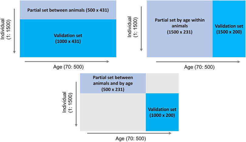
Figure 1. Outline of three data partitioning scenarios to create partial and validation sets for the LR method.
LR method
As described below, following Legarra and Reverter (2018), two statistics are used to check whether the model is adequate.
1. The first statistic is
2. The second statistic is obtained by regressing
This estimator was referred to as an estimator of dispersion by Legarra and Reverter (2018) and of inflation by Belay et al. (2022), where 1 indicates no bias. Suppose animals are selected based on EBV to increase the values of a trait. Then if the true regression coefficient is less than 1, the BV of selected candidates is expected to be lower than their EBV, which indicates an upward bias of the EBV of the selected animals. On the other hand, when
Provided the model is adequate, in the LR method, population accuracy is estimated as
In addition to
The means of Δ and
Results
To visualize the prediction performances across the fitted models and partitioning scenarios, we randomly picked one individual from the validation set and displayed its simulated data against its predictions in Figure 2. Both simulated body weight phenotypes, true BV, and EBV of the selected individual were displayed. The predicted data included the EBV based on the partial and the whole data sets for the three partitioning scenarios (Figure 2).
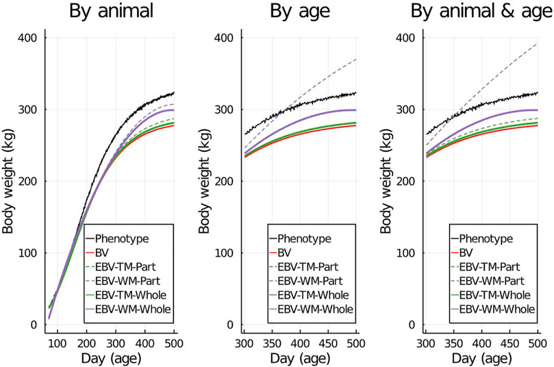
Figure 2. An example showing one randomly selected individual’s simulated phenotypes, true breeding values (BV), and estimated breeding values (EBV) for body weight by age using the true model (TM) and the wrong model (WM) when the data set was partitioned using different scenarios.
Evaluating model adequacy
Figure 3 shows the Δ and
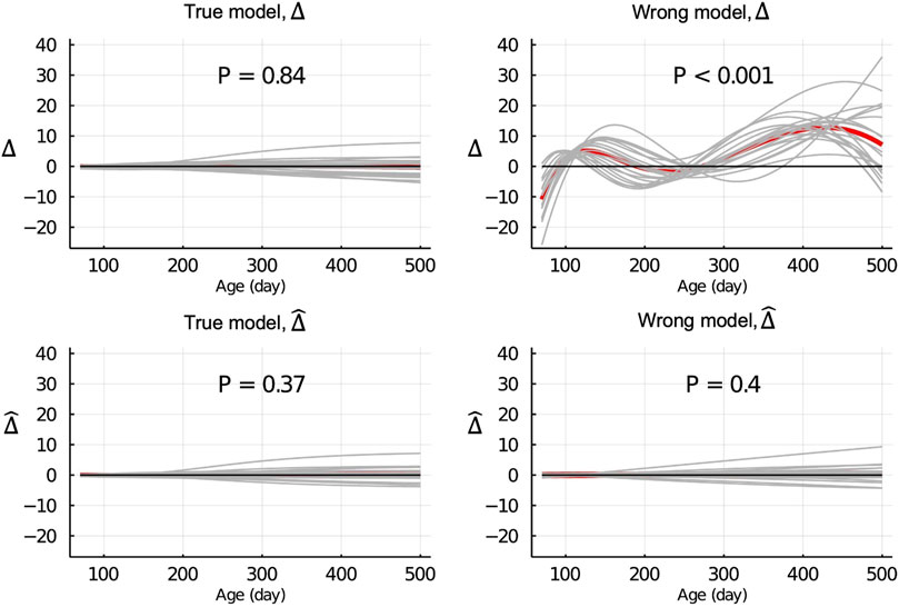
Figure 3.
Figure 4 shows the Δ and
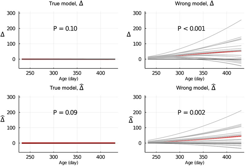
Figure 4.
Figure 5 shows the true and LR estimates of the regression coefficient of EBV for body weights for each day when the data were partitioned between animals. When the true model was used, both the true and estimated regression coefficients were symmetrically distributed around 1 for each day, and their mean was not significantly different from 1 (p = 0.75 and = 0.53, respectively). When the wrong model was used, the true and LR estimates of the regression coefficient were significantly different from 1 (p < 0.001). Results for the partitioning by age within animals and between animals and by age were consistent with those in Figure 5 and are given in Figure 6; Supplementary Figure S2, respectively.
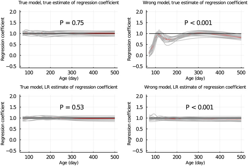
Figure 5. True and LR estimates of regression coefficient of EBV of body weights for each day of age when the true or wrong model was fitted and when partitioning the data between animals. The true and LR estimates of regression coefficient are defined by regressing u on
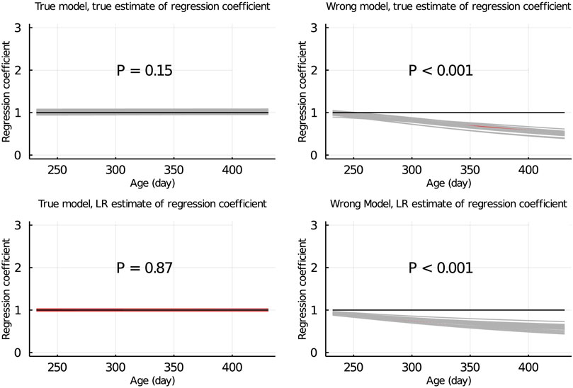
Figure 6. True and LR estimates of regression coefficient of EBV of body weights for each day of age when the true or wrong model was fitted and when partitioning the data by age within animals. The true and LR estimates of regression coefficient are defined by regressing u on
Population accuracy
In Figure 7, the true and LR estimates of prediction accuracy of EBV for body weights for each day when the data were partitioned between animals are presented. The LR estimates of prediction accuracy had a similar pattern as the true estimates of accuracy when using the true model but not when the wrong model was used. When partitioning the data by age within animals, the LR estimates of accuracy showed a similar pattern as the true estimates of accuracy, regardless of the model fitted (Figure 8). We also evaluated the difference between
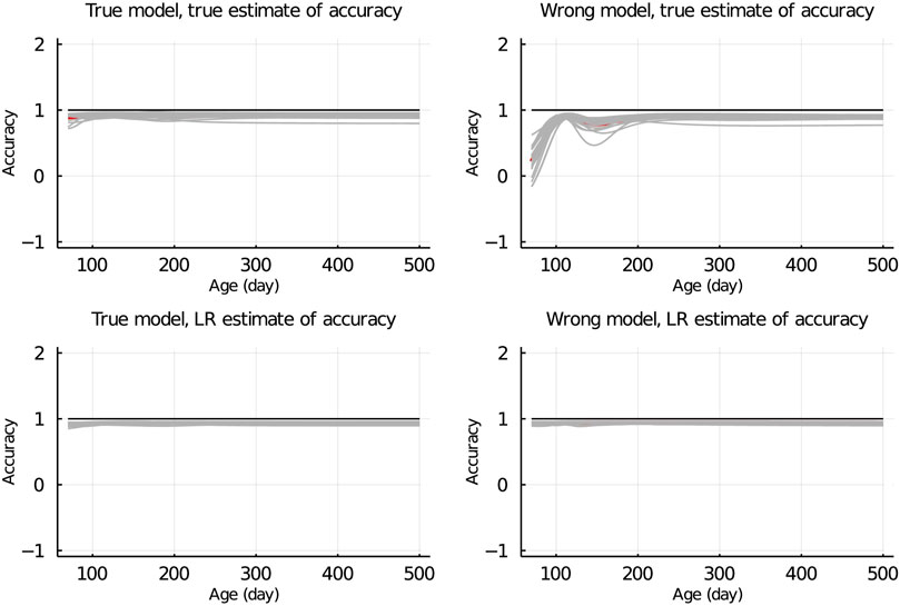
Figure 7. True and LR estimates of accuracy when the true or wrong model was fitted and when partitioning the data between animals. The true accuracy is defined as the correlation between true breeding values u and estimated breeding values of validation set based on partial set
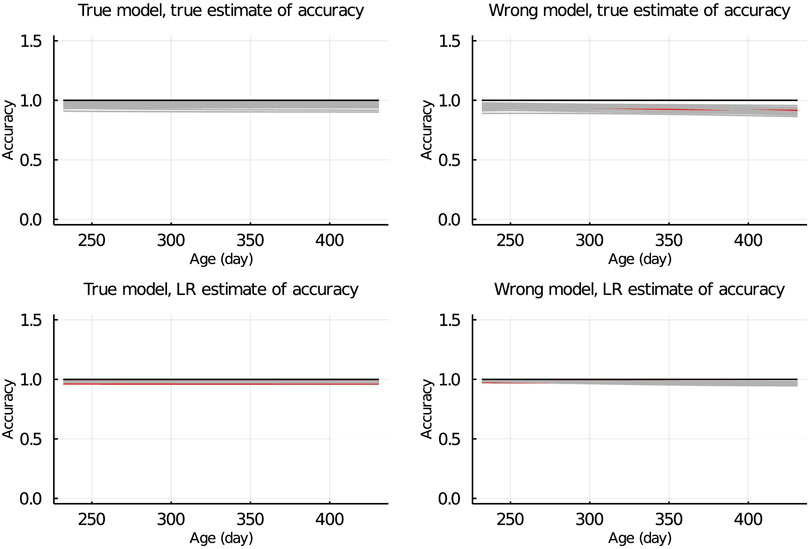
Figure 8. True and LR estimates of accuracy when the true or wrong model was fitted and when partitioning the data by age within animals. The true accuracy is defined as the correlation between true breeding values u and estimated breeding values of validation set based on partial set
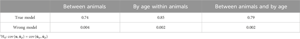
Table 1. Significance (p-values) of tests1 for the difference between
Discussion
Based on the initial idea by Reverter et al. (1994), Legarra and Reverter (2018) proposed the LR method to quantify the population accuracy of prediction of EBV implicitly assuming the fitted model is correct. They proved the validity of the LR method for EBV from a linear model using standard BLUP theory and applied the LR method to a real cattle data set (Legarra and Reverter, 2018). While the LR method has also been applied to EBV from a threshold model (Bermann et al., 2021), a mathematical proof of its validity for a non-linear method of prediction was not previously available. In this paper we provide the justification of the LR method for non-linear predictions.
The motivation for this paper came from a discussion on the validity of using the LR method to evaluate the prediction performance from a non-linear growth model, where marker effects are linked to body weight through latent variables. In this case, traditional CV cannot be used to obtain the accuracy of the latent variables because phenotypes are not available for these variables. However, in the LR method,
Use of the LR method to estimate accuracy of prediction when the model is adequate
To generalize the LR method for linear or non-linear predictions, we presented a mathematical proof to justify using
Use of the LR method to test model adequacy
We used simulated longitudinal data to investigate the ability of the LR method to determine whether the fitted model is adequate. In the context of our situation, the non-linear relationship is between the age of the animal and its weight, which makes how the data are partitioned into training and validation sets important. To explore how the strategy for partitioning the data into training and validation sets affects the ability of the LR method to determine whether the fitted model is adequate, three data partitioning strategies were used: between animals, by age within animals, and between animals and by age. We did not simulate selection in our data because we were comparing two models of growth rather than two models of inheritance. When the fitted model for growth is not adequate and the data are partitioned by age within animals, predictions from the training data would not be accurate even without selection. Thus, selection was not required to investigate properties of the LR method in this context. Further, in our analysis of the simulated data, the QTL were used as markers, for simplicity, but this does not influence the conclusions of our study either.
Effect of data partitioning strategy on test of model adequacy
Below, we summarize the implications of the data partitioning strategies on the performance of the LR method, thereby providing guidelines for using the
When the wrong model (BHQGM) was fitted and the data were partitioned between animals, the Δ was significant, but the
Recall that in the LR method, the regression of u on
When the data were partitioned by age within animals, the LR method was able to correctly detect that the model was inadequate using
The inconsistency between
Guidelines for data partitioning
In general, to properly test the model adequacy using the LR method, we need to use the model to predict the performance of individuals that have values for the relevant predictor variables or combination of predictor variables that were not present in the training data. In our simulated data, the predictor variables included the marker genotypes, as well as age. Let’s define the predicted performance of individual i as
Conclusion
We provide a mathematical proof for the validity of the LR method to estimate the accuracy of predictions based on the conditional mean, regardless of whether predictions are a linear or non-linear function of data, provided the fitted model is adequate. In the LR method, two statistics are used to check model adequacy. We found that the
Data availability statement
The original contributions presented in the study are included in the article/Supplementary Material, further inquiries can be directed to the corresponding authors.
Author contributions
HY: Writing–original draft, Writing–review and editing. RF: Writing–original draft, Writing–review and editing. JD: Writing–original draft, Writing–review and editing.
Funding
The author(s) declare that financial support was received for the research, authorship, and/or publication of this article. This work was funded by USDA National Institute of Food and Agriculture award number 2020-67015-31031.
Conflict of interest
The authors declare that the research was conducted in the absence of any commercial or financial relationships that could be construed as a potential conflict of interest.
The author(s) declared that they were an editorial board member of Frontiers, at the time of submission. This had no impact on the peer review process and the final decision.
Publisher’s note
All claims expressed in this article are solely those of the authors and do not necessarily represent those of their affiliated organizations, or those of the publisher, the editors and the reviewers. Any product that may be evaluated in this article, or claim that may be made by its manufacturer, is not guaranteed or endorsed by the publisher.
Supplementary material
The Supplementary Material for this article can be found online at: https://www.frontiersin.org/articles/10.3389/fgene.2024.1380643/full#supplementary-material
SUPPLEMENTARY FIGURE S1 |
SUPPLEMENTARY FIGURE S2 | True and LR estimates of regression coefficient of EBV of body weights at each day when the true or wrong model was fitted and when partitioning the data between animals and by age. The true and LR estimates of regression coefficient are defined by regressing u on
SUPPLEMENTARY FIGURE S3 | True and LR estimates of accuracy of EBV of body weights at each day when the true or wrong model was fitted and when partitioning the data between animals and by age. The true accuracy is defined as the correlation between true breeding values u and estimated breeding values of validation set based on partial set
References
Belay, T. K., Eikje, L. S., Gjuvsland, A. B., Nordbø, Ø., Tribout, T., and Meuwissen, T. (2022). Correcting for base-population differences and unknown parent groups in single-step genomic predictions of Norwegian red cattle. J. Anim. Sci. 100, skac227. doi:10.1093/jas/skac227
Bermann, M., Legarra, A., Hollifield, M. K., Masuda, Y., Lourenco, D., and Misztal, I. (2021). Validation of single-step gblup genomic predictions from threshold models using the linear regression method: an application in chicken mortality. J. Anim. Breed. Genet. 138, 4–13. doi:10.1111/jbg.12507
Bernardo, R., and Yu, J. (2007). Prospects for genomewide selection for quantitative traits in maize. Crop Sci. 47, 1082–1090. doi:10.2135/cropsci2006.11.0690
Bezanson, J., Edelman, A., Karpinski, S., and Shah, V. B. (2017). Julia: a fresh approach to numerical computing. SIAM Rev. Soc. Ind. Appl. Math. 59, 65–98. doi:10.1137/141000671
Brossard, L., Dourmad, J. Y., Rivest, J., and van Milgen, J. (2009). Modelling the variation in performance of a population of growing pig as affected by lysine supply and feeding strategy. animal 3, 1114–1123. doi:10.1017/S1751731109004546
Cai, W., Kaiser, M., and Dekkers, J. (2012). Bayesian analysis of the effect of selection for residual feed intake on growth and feed intake curves in yorkshire swine. J. animal Sci. 90 (1), 127–141. doi:10.2527/jas.2011-4293
Dekkers, J., and Hospital, F. (2002). The use of molecular genetics in the improvement of agricultural populations. Nat. Rev. Genet. 3, 22–32. doi:10.1038/nrg701
Fernando, R., Cheng, H., Sun, X., and Garrick, D. (2017). A comparison of identity-by-descent and identity-by-state matrices that are used for genetic evaluation and estimation of variance components. J. Animal Breed. Genet. 134 (3), 213–223. doi:10.1111/jbg.12275
Fernando, R., and Gianola, D. (1986). Optimal properties of the conditional mean as a selection criterion. Theor. Appl. Genet. 72, 822–825. doi:10.1007/BF00266552
Habier, D., Fernando, R. L., Kizilkaya, K., and Garrick, D. J. (2011). Extension of the bayesian alphabet for genomic selection. BMC Bioinforma. 12, 1–12. doi:10.1186/1471-2105-12-186
Henderson, C. (1982). Best linear unbiased prediction in populations that have undergone selection. in Proceedings of the world congress on sheep and beef cattle breeding (Palmerston North, New Zealand: Dunmore Press), Vol. 28.
Legarra, A., and Reverter, A. (2018). Semi-parametric estimates of population accuracy and bias of predictions of breeding values and future phenotypes using the lr method. Genet. Sel. Evol. 50, 53–18. doi:10.1186/s12711-018-0426-6
Legarra, A., Robert-Granié, C., Manfredi, E., and Elsen, J.-M. (2008). Performance of genomic selection in mice. Genetics 180 (1), 611–618. doi:10.1534/genetics.108.088575
Macedo, F., Reverter, A., and Legarra, A. (2020). Behavior of the linear regression method to estimate bias and accuracies with correct and incorrect genetic evaluation models. J. Dairy Sci. 103, 529–544. doi:10.3168/jds.2019-16603
Meuwissen, T. H., Hayes, B. J., and Goddard, M. (2001). Prediction of total genetic value using genome-wide dense marker maps. Genetics 157, 1819–1829. doi:10.1093/genetics/157.4.1819
Morota, G., and Gianola, D. (2014). Kernel-based whole-genome prediction of complex traits: a review. Front. Genet. 5, 363. doi:10.3389/fgene.2014.00363
Morota, G., Koyama, M., M Rosa, G. J., Weigel, K. A., and Gianola, D. (2013). Predicting complex traits using a diffusion kernel on genetic markers with an application to dairy cattle and wheat data. Genet. Sel. Evol. 45, 17–15. doi:10.1186/1297-9686-45-17
Reverter, A., Golden, B., Bourdon, R., and Brinks, J. (1994). Technical note: detection of bias in genetic predictions. J. Anim. Sci. 72, 34–37. doi:10.2527/1994.72134x
Saatchi, M., McClure, M. C., McKay, S. D., Rolf, M. M., Kim, J., Decker, J. E., et al. (2011). Accuracies of genomic breeding values in american angus beef cattle using k-means clustering for cross-validation. Genet. Sel. Evol. 43, 40–16. doi:10.1186/1297-9686-43-40
Serão, N. V., Kemp, R. A., Mote, B. E., Willson, P., Harding, J., Bishop, S. C., et al. (2016). Genetic and genomic basis of antibody response to porcine reproductive and respiratory syndrome (prrs) in gilts and sows. Genet. Sel. Evol. 48, 51–15. doi:10.1186/s12711-016-0230-0
Utz, H. F., Melchinger, A. E., and Schön, C. C. (2000). Bias and sampling error of the estimated proportion of genotypic variance explained by quantitative trait loci determined from experimental data in maize using cross validation and validation with independent samples. Genetics 154, 1839–1849. doi:10.1093/genetics/154.4.1839
Varona, L., Moreno, C., Cortes, L. G., Yagüe, G., and Altarriba, J. (1999). Two-step versus joint analysis of von bertalanffy function. J. Animal Breed. Genet. 116 (5), 331–338. doi:10.1046/j.1439-0388.1999.00220.x
Wolc, A., Stricker, C., Arango, J., Settar, P., Fulton, J. E., O’Sullivan, N. P., et al. (2011). Breeding value prediction for production traits in layer chickens using pedigree or genomic relationships in a reduced animal model. Genet. Sel. Evol. 43, 5–9. doi:10.1186/1297-9686-43-5
Keywords: conditional mean, linear regression method, model adequacy, non-linear model, population accuracy
Citation: Yu H, Fernando RL and Dekkers JCM (2024) Use of the linear regression method to evaluate population accuracy of predictions from non-linear models. Front. Genet. 15:1380643. doi: 10.3389/fgene.2024.1380643
Received: 01 February 2024; Accepted: 06 May 2024;
Published: 31 May 2024.
Edited by:
Li Ma, University of Maryland, United StatesReviewed by:
Juliana Petrini, University of São Paulo, BrazilSajjad Toghiani, Agricultural Research Service (USDA), United States
Copyright © 2024 Yu, Fernando and Dekkers. This is an open-access article distributed under the terms of the Creative Commons Attribution License (CC BY). The use, distribution or reproduction in other forums is permitted, provided the original author(s) and the copyright owner(s) are credited and that the original publication in this journal is cited, in accordance with accepted academic practice. No use, distribution or reproduction is permitted which does not comply with these terms.
*Correspondence: Haipeng Yu, aGFpcGVuZ3l1QHVmbC5lZHU=; Jack C. M. Dekkers, amRla2tlcnNAaWFzdGF0ZS5lZHU=