Abstract
Single-step genomic BLUP (ssGBLUP) model for routine genomic prediction of breeding values is developed intensively for many dairy cattle populations. Compatibility between the genomic (G) and the pedigree (A) relationship matrices remains an important challenge required in ssGBLUP. The compatibility relates to the amount of missing pedigree information. There are two prevailing approaches to account for the incomplete pedigree information: unknown parent groups (UPG) and metafounders (MF). unknown parent groups have been used routinely in pedigree-based evaluations to account for the differences in genetic level between groups of animals with missing parents. The MF approach is an extension of the UPG approach. The MF approach defines MF which are related pseudo-individuals. The MF approach needs a Γ matrix of the size number of MF to describe relationships between MF. The UPG and MF can be the same. However, the challenge in the MF approach is the estimation of Γ having many MF, typically needed in dairy cattle. In our study, we present an approach to fit the same amount of MF as UPG in ssGBLUP with Woodbury matrix identity (ssGTBLUP). We used 305-day milk, protein, and fat yield data from the DFS (Denmark, Finland, Sweden) Red Dairy cattle population. The pedigree had more than 6 million animals of which 207,475 were genotyped. We constructed the preliminary gamma matrix (Γpre) with 29 MF which was expanded to 148 MF by a covariance function (Γ148). The quality of the extrapolation of the Γpre matrix was studied by comparing average off-diagonal elements between breed groups. On average relationships among MF in were 1.8% higher than in Γpre. The use of Γ148 increased the correlation between the G and A matrices by 0.13 and 0.11 for the diagonal and off-diagonal elements, respectively. [G]EBV were predicted using the ssGTBLUP and Pedigree-BLUP models with the MF and UPG. The prediction reliabilities were slightly higher for the ssGTBLUP model using MF than UPG. The ssGBLUP MF model showed less overprediction compared to other models.
1 Introduction
Genomic prediction in dairy cattle started in 2009 for US Holsteins, Jersey, and Brown Swiss (Wiggans et al., 2017). Since then, most dairy populations publish genomic estimated breeding values (GEBV) using a multi-step approach (Masuda et al., 2022). The term “multi” stands for a cascade of steps used to obtain GEBV: calculation of pseudo-observations for genotyped proven bulls and cows, estimation of SNP effects, prediction of direct genomic values, and blending of genomic values with pedigree index (Wiggans et al., 2011). In contrast, a single-step genomic BLUP (ssGBLUP) model accounts for pedigree, phenotypic, and genomic data simultaneously to obtain GEBVs for all animals (Legarra et al., 2009; Aguilar et al., 2010; Christensen and Lund, 2010). Despite the preselection bias in the multi-step GEBV (Patry and Ducrocq, 2011) and the benefits of the single-step model (Legarra et al., 2014), the latter is used only for a few dairy populations (Mäntysaari et al., 2020; Misztal et al., 2020; Masuda et al., 2022). High computational load, compatibility challenges for the genomic and the pedigree relationship matrices, and improper accounting of unknown parents impede the wide implementation of the single-step approach (Mäntysaari et al., 2020). In dairy cattle, these problems can be expected to be amplified due to the many generations in pedigrees, intensive selection, and the vast exchange of breeding material between populations.
The original ssGBLUP requires the inverse matrices of A22 and G in the inverted joint relationship matrix H−1 (Aguilar et al., 2010; Christensen and Lund, 2010) where A22 is the pedigree relationship matrix of the genotyped animals and G is the genomic relationship matrix. When the number of genotyped animals in the G matrix (n) exceeds the number of markers (m), direct inversion of the G matrix is not possible without regularization such as adding a small value to the diagonal or a residual polygenic matrix (Mäntysaari et al., 2017). When n >> m, the single-step method becomes computationally challenging. Several computational approaches have been proposed for the computation of G−1 to allow feasible application of ssGBLUP for large datasets (see review by Misztal et al., 2020). For instance, the method called ssGTBLUP (Mäntysaari et al., 2017) uses the relationship matrix of genotyped animals (A22) as the regularization matrix to avoid singularity, the Woodbury matrix identity for the G inverse, and a sparse presentation of the A22−1 to solve the computational challenges. In the data set with 178K genotyped animals to obtain GEBV, the ssGTBLUP model used 33% of the memory and 55% of the wall-clock time needed by the original ssGBLUP (Koivula et al., 2021a).
The difference in average off- and diagonal elements of A22 and G matrices is known as a single-step compatibility issue (Vitezica et al., 2011). To balance the matrices implies adjusting either the pedigree or the genomic relationship matrix to make the matrices more similar. The concept of the A adjustment was suggested by Christensen (2012) and further developed into the metafounder (MF) approach (Legarra et al., 2015). Metafounders are related inbreed pseudo-individuals that are used as unknown parents in the pedigree. Relationships between MF are described by a covariance matrix (Γ), which is used to build a relationship matrix AΓ. Estimation of Γ can be based on estimates of base allele frequencies (AF) for each MF (Garcia-Baccino et al., 2017). An important assumption of the MF approach is that the G matrix is constructed with all AF equal to 0.5 (Legarra et al., 2015). Applicability of MF has been shown in livestock (Koivula et al., 2021b, 2022), sheep (Granado-Tajada et al., 2020), and pig (Xiang et al., 2017) data sets. The MF approach was also reported as a perfect choice for multi-breed evaluations in case computation of accurate Γ is possible (Poulsen et al., 2022).
The number of MF in the reported studies on ssGBLUP in the large dairy cattle breeds has nearly always been less than the number of unknown parent groups (UPG). Allocation of few MF by breed or by breed by time help to achieve an accurate estimation of Γ due to the even distribution of MF across genotyped animals (Kudinov et al., 2020; Masuda et al., 2021). When MF are used in ssGBLUP, it would be natural to use the same number of MF as there are UPG in the pedigree-based animal model (PBLUP). However, accurate estimation of an unstructured Γ matrix of large size is difficult, especially if some of the UPG groups have no descendants among the genotyped animals or genotyped individuals are several generations away.
The aim of this study was to propose an approach to construct Γ with the same number of MF as routinely defined UPG. The proposed approach was applied to the Red Dairy Cattle 305-day data and pedigree used for the milk production evaluation in Nordic countries (Denmark, Finland, and Sweden). Both PBLUP and ssGTBLUP models were used. The predictions used either UPG or MF in equal numbers. Thus, the predictive performance of four models was investigated.
2 Materials and methods
2.1 Data
Data were 305-day milk, protein, and fat yield records from three lactations of Nordic Red Dairy Cattle (RDC), Finnish Holstein (HOL), and Finncattle (FIC) cows. Records were from January 1988 to June 2021. The total number of records by trait were: 9.45, 8.99, and 8.98 million for milk, protein, and fat, respectively (Table 1). Pedigree included 6.05 million cows and 118,363 bulls, of which 8,427 were RDC and 278 were FIC proven bulls. Genetic groups were defined as breed x country x five- or 10-year period for RDC, and as breed x five- or 10-year period for HOL, FIC, and other breeds. In total, there were 148 groups: 61 RDC, 45 HOL, 16 FIC, and 26 for breed group OTHER. The group OTHER included 23 breeds majorly beef cattle.
TABLE 1
| RDCa | HOLb | FICc | |||||||
|---|---|---|---|---|---|---|---|---|---|
| Lactation | I | II | III | I | II | III | I | II | III |
| Milk | 3,468,211 | 2,516,689 | 1,546,056 | 837,905 | 628,763 | 394,169 | 27,620 | 19,227 | 12,103 |
| Protein | 3,362,027 | 2,414,026 | 1,466,707 | 771,209 | 567,914 | 349,911 | 24,999 | 17,381 | 10,896 |
| Fat | 3,361,935 | 2,413,956 | 1,466,662 | 771,214 | 567,913 | 349,911 | 24,999 | 17,382 | 10,896 |
Number of records by lactation, trait, and breed in 305-day Nordic (Denmark, Finland, Sweden) Red Dairy cattle production data.
Red Dairy cattle.
Finnish Holstein.
Finncattle.
Genomic data were used from 206,140 RDC animals (6,018 proven bulls and 85,142 cows with records) and 1,335 FIC animals (160 proven bulls and 845 cows with records). Before 2019 the bulls were genotyped with Illumina Bovine SNP50 array and most cows with Illumina Bovine LD array (Illumina, San Diego, CA, USA). Since 2019 both bulls and cows were genotyped with Eurogenomics EG MD array (https://www.eurogenomics.com/). Quality control and imputation of genotypes to 46,914 SNPs were performed by NAV (Nordic Genetic Evaluation, Denmark). Genomic markers were not filtered on minor allele frequency and no edits were done concerning across and within breeds polymorphism. HOL genotypes were not presented in the current study.
2.2 Statistical models
Four prediction models were investigated using a multi-trait multi-lactation model: single-step GTBLUP with UPG in H−1 (ssUPG), single-step GTBLUP with MF (ssMF), pedigree-based BLUP with UPG in A−1 (pUPG), and pedigree-based BLUP with MF (pMF). The traits were milk, protein, and fat yield in three lactations i.e. - nine traits total. The linear mixed effects model was:where y is the vector of phenotypes, X is the design matrix relating fixed effects to the phenotypes, b is the vector of fixed effects, Z is the design matrix relating the breeding values to the phenotypes, is the vector of random animal breeding values, and is the residual vector. Matrix A is the pedigree-based relationship matrix, is an identity matrix, and are genetic and residual variances, respectively. Fixed effects in b were calving year by season, calving age, herd by year, and calving age by breed. Calving age by breed effect consists of linear (α), quadratic (α2), and cubic (α3) regression coefficients of calving age multiplied by pedigree-based breed proportions of an animal (Lidauer et al., 2015) so that the general level of breed remained to be modeled by u. The regression coefficients were centered over all data to zero according to mean calving age as .
2.2.1 Single-step GTBLUP
The mixed model equations (MME) of the original ssGBLUP model require the inverse of a joint relationship matrix H−1 (Aguilar et al., 2010; Christensen and Lund, 2010):where, A22 is the part in A for the genotyped animals, and G is the genomic relationship matrix (VanRaden, 2008). Regularization matrix C = wA22 was added to the marker-based matrix G, where w is the residual polygenic proportion, i.e., the genomic relationship matrix was Gc_w = (1-w)G+ wA22 (Mäntysaari et al., 2017). We used w equal to 30% to keep the comparability to the studies by Koivula et al. (2021b, 2022). The Gc_w matrix was constructed with the assumption that AF of all markers was equal to 0.5. Thus, Gc_w = (1-w)Z101Z101´/k + wA22 where k = m/2 is the scaling factor, m is the number markers, and Z101 is the matrix of genotype counts with values of 0 for the heterozygote and values -1 and +1 for homozygotes. The inverse genomic relationship matrix can be expressed as (Mäntysaari et al., 2017) where and Lw is the Cholesky decomposition of .
2.2.2 Single-step GTBLUP with UPG
The joint relationship matrix augmented by UPG (Quaas and Pollak, 1981; Misztal et al., 2013; Matilainen et al., 2018) was computed as shown in Koivula et al. (2021a):where and
The Q matrix has proportions of genes contributed from each UPG according to pedigree information. The subscripts 1 and 2 in Q pertain to genotyped and non-genotyped animals. Subscripts 1 and 2 in B pertain to genotyped animals and UPGs, respectively. The UPGs were modeled as random effect. Inbreeding coefficients were accounted in both pedigree-based relationship matrices.
2.2.3 Single-step GTBLUP with MF
In the MF approach (Christensen, 2012; Legarra et al., 2015), the H−1 matrix was replaced by:where Gc_w=(1-w)G+ w, AΓ is pedigree relationship matrix formed with a Γ matrix, is the submatrix of AΓ for the genotyped animals, and Γ was variance covariance matrix of the MF. Inbreeding coefficients estimated using the Γ matrix were used in the inverses of and .
2.2.4 Pedigree BLUP
The pedigree-based models (pUPG and pMF) were similar to their corresponding single-step models, except that the genomic data was excluded from the prediction. In pUPG model UPGs were accounted in A−1 (;Quaas and Pollak, 1981). In pMF model the A−1 was replaced by .
2.5 Estimation of the Γ matrix
Let the number of MF be
rsuch that the
Γmatrix has size
r. In the MF approach, the
Γmatrix describes the variance-covariance structure of MF. It can be estimated by
, where
Pis an
mby
rmatrix of estimated base population AF for each marker and MF (
Legarra et al., 2015;
Garcia-Baccino et al., 2017). In the studied data set, 44% of the UPG were not linked to the genotypes. Thus, using the 148 UPG as MF in the estimation of
Pwas not feasible. To compute
Γfor a large number of MF, the following general steps were used:
a) Estimate allele frequencies for a set of base groups;
b) From estimated allele frequencies, calculate the preliminary Γ matrix (Γpre) for the base groups;
c) Solve the matrix K in the covariance function Γpre= + E using Γpre and the model matrix Φpre; The matrix E is null if row rank of is equal to dimension of Γpre and, if not E represents least squares errors of estimation.
d) Compute the Γ for the large number of groups as .
The model matrices and define linear model by group and time for the set of base MF and for all MF, respectively.
The technical detailed steps used to compute
Γfor 148 groups (
Γ148) were:
a) The pedigree was pruned to include only one ancestor generation of genotyped animals as in Kudinov et al. (2020). Truncation of the pedigree helped to achieve equal distribution of the genomic information over UPGs. Missing parents in the truncated pedigree were replaced by 26 groups formed by breed, country, and time interval (Table 2). All HOL ancestors were assigned to the same group regardless of country and time. Estimation of base population AF for each of the groups (PRDC) was performed using the GLS method (McPeek et al., 2004; Garcia-Baccino et al., 2017). The HOL group estimated from RDC genotypes was dropped from PRDC. The HOL AF (PHOL) were the same as used in Kudinov et al. (2020)—calculated using Holstein genotypes (M. Koivula, personal communication). The joint PRDC_HOL matrix of size 29 by 45,823 was created by merging compatible SNPs in PRDC and PHOL. Number of SNPs dropped from PRDC and PHOL where 1,091 and 519, respectively.
b) Three Γ matrices (ΓRDC_HOL, ΓRDC, and ΓHOL) were computed using PRDC_HOL, PRDC, and PHOL. A pre-Γ matrix (Γpre, Figure 1) was created by replacing the diagonal elements of ΓRDC_HOL by diagonal elements of ΓRDC and ΓHOL at corresponding places. The diagonal values in Γpre were larger than in ΓRDC_HOL.
c) Structure of Γpre was computed with covariance function (Kirkpatrick et al., 1990), where Φprewas a model matrix having standardized year of the MF (Appendix 1) and K was a matrix of co-variance function coefficients. Year standardization was done using formula , where yearMF is a year of the MF, yearmin and yearmax are the first (1950) and the last (2021) year points among the 148 groups in the pedigree.
TABLE 2
| Breeda | Originb | Birth years of the animals descending from the group (MF) | Abbreviation | Genotype setc | Proportion of genotyped animals tied to the group (%)d |
|---|---|---|---|---|---|
| RDC | FIN | <1970 | FIN70 | RDC | 3.62 |
| RDC | FIN | 1971–1980 | FIN80 | RDC | 7.35 |
| RDC | FIN | 1981–1990 | FIN90 | RDC | 7.91 |
| RDC | FIN | 1991–2000 | FIN00 | RDC | 6.17 |
| RDC | FIN | 2001–2010 | FIN10 | RDC | 7.29 |
| RDC | FIN | 2011–2020 | FIN20 | RDC | 1.51 |
| RDC | SWE | <1970 | SWE70 | RDC | 4.20 |
| RDC | SWE | 1971–1980 | SWE80 | RDC | 6.85 |
| RDC | SWE | 1981–1990 | SWE90 | RDC | 11.00 |
| RDC | SWE | 1991–2000 | SWE00 | RDC | 8.68 |
| RDC | SWE | 2001–2010 | SWE10 | RDC | 1.14 |
| RDC | SWE | 2011–2020 | SWE20 | RDC | 0.22 |
| RDC | DNK | <1980 | DNK80 | RDC | 2.17 |
| RDC | DNK | 1981–1990 | DNK90 | RDC | 3.76 |
| RDC | DNK | 1991–2000 | DNK00 | RDC | 4.26 |
| RDC | DNK | 2001–2010 | DNK10 | RDC | 4.61 |
| RDC | DNK | 2011–2020 | DNK20 | RDC | 0.80 |
| RDC | NOR | <2000 | NOR00 | RDC | 4.51 |
| RDC | NOR | 2001–2020 | NOR20 | RDC | 0.24 |
| RDC | ANY | <2000 | RDC00 | RDC | 5.93 |
| RDC | ANY | 2001–2020 | RDC20 | RDC | 1.20 |
| FIC | FIN | <1990 | FIC90 | RDC | 0.37 |
| FIC | FIN | 1991–2000 | FIC00 | RDC | 0.15 |
| FIC | FIN | 2000–2020 | FIC20 | RDC | 0.12 |
| OTHER | ANY | <2020 | OTH20 | RDC | 2.60 |
| HOL | ANY | <1970 | HOL70 | HOL | 13.42 |
| HOL | ANY | 1971–1990 | HOL90 | HOL | 6.35 |
| HOL | ANY | 1991–2010 | HOL10 | HOL | 3.06 |
| HOL | ANY | 2010–2020 | HOL20 | HOL | 1.41 |
Groups used to compute preliminary Γ matrix.
Breeds were RDC, Read Dairy Cattle; FIC, Finncattle; HOL, Holstein, and OTHER, other than listed.
Countries of origin: FIN, Finland; SWE, Sweden; DNK, Denmark; NOR, Norway, and ANY, any than specially specified.
RDC, and HOL, genotypes set include 46,914 and 46,342 markers, respectively. RDC, set included FIC, genotypes imputed along with RDC, genotypes.
Proportion of genotypes tied to the group in a particular genotype set.
FIGURE 1
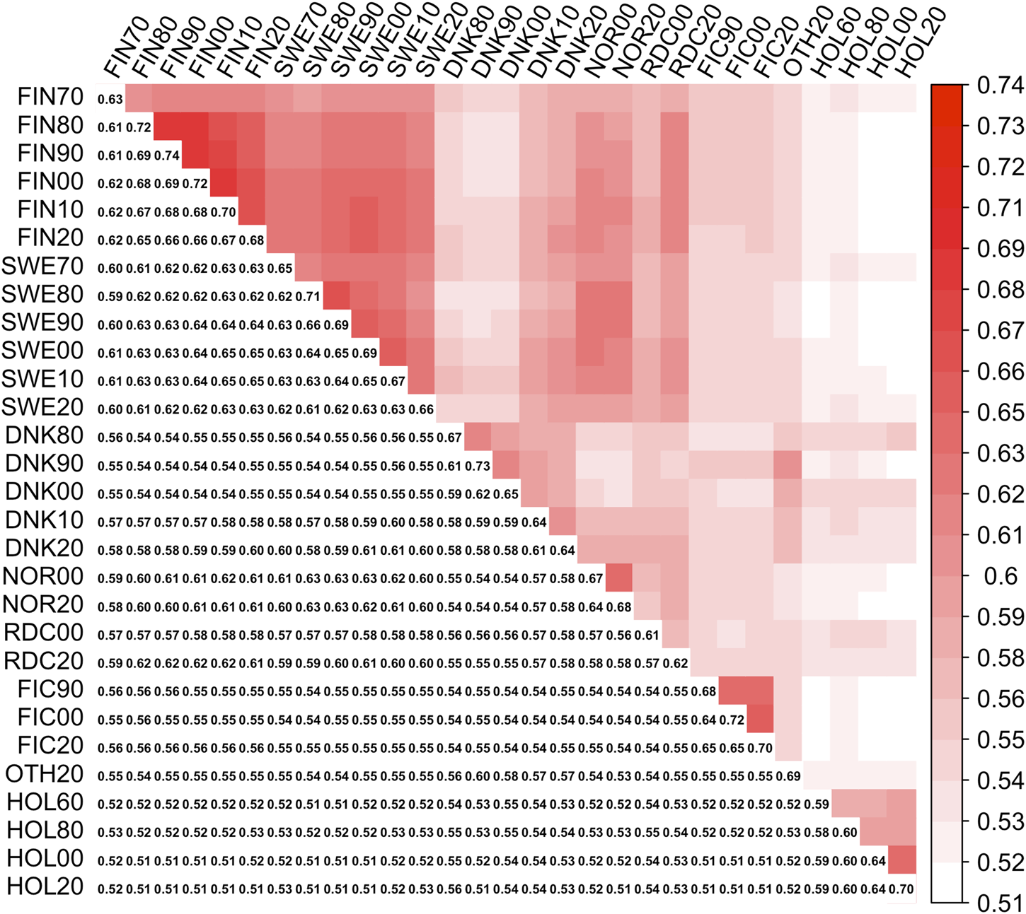
Symmetrical covariance matrix between 29 MFs (Γpre). Lower triangle present diagonal (MFs self-relationships) and off-diagonal (between MFs relationships) elements in Γpre upper triangle—heatmap plot of the off-diagonals.
Matrix
Kwas estimated as (
Tijani et al., 1999):
leading to estimate
d) Finally, the Γ148 was estimated as , where the matrix Φ148 was designed same way as Φpre but using all the MF. Rank of the Γ148 matrix is only 9. To avoid AΓ matrix singularity we reduced the off-diagonal values of Γ148 by 2.5% and increased the diagonal values by 2.5%
2.6 Validation of model fit
Validation of the prediction models was done using modified forward prediction (Mäntysaari et al., 2010). For the validation a reduced phenotypic data set was constructed by removing records from the last 4 years of data, i.e., June 2017 to June 2021. Daughter yield deviations (DYD) for bulls and yield deviations (YD) for cows were computed using the full data set using the same model which was applied to reduced data. Bias of evaluation was estimated by the linear regression coefficient (b1) from the weighted regression of DYD/YD on the corresponding [G]EBV predicted with the reduced data. The weight of DYD for bull i was EDCi/(EDCi + λb), where λb is (4—h2)/h2, h2 is heritability of the trait, and EDCi is the effective daughter contributions of bull i computed as in Taskinen et al. (2014). Weight for cow YDj was computed as ERCj/(ERCj + λc), where λc is (1-h2)/h2 and ERCj is the effective record contribution of cow j (Přibyl et al., 2013). Adjusted validation reliability was attained by dividing the coefficient of determination from the regression model () by the average weight of DYD () and YD () for bulls and cows, respectively. Average genetic trends were plotted using the trait specific combined [G]EBVs computed as(https://nordicebv.info/wp-content/uploads/2021/10/NAV-routine-genetic-evaluation_EDITYSS-08102021.pdf).
2.7 Software
Pedigree truncation and estimation of the inbreeding coefficients was done using RelaX2 v.1.95 software. The AF were estimated using Bpop v. 0.98 program (Strandén and Vuori, 2006; Strandén and Mäntysaari, 2020), T matrix and its diagonal needed in the ssGTBLUP model were computed using hgtinv v.0.83 program. The computation of [G]EBV predictions and the estimation of EDC/ERC used MiX99 software (Strandén and Lidauer, 1999). MiX99 software uses preconditioned conjugate gradient (PCG) iteration. The PCG method was assumed to be converged when convergency criteria <1e-6 was achieved. Convergency criteria was defined as a Euclidean norm of the difference between the right-hand side (RHS) of the MME and the one predicted by the current solutions relative to the norm of RHS. The matrices and used by MiX99 and hginv were constructed using the given pedigree and inbreeding files, and in case of MF, by file with the Γ−1 matrix.
3 Results and discussion
3.1 Relationship matrices
Elements of Γpre ranged from 0.59 to 0.74 and from 0.51 to 0.69 for the diagonal and off-diagonal elements, respectively. The lowest and highest diagonal values (self-relationship, Legarra et al., 2015) were in groups HOL 1960 and RDC FIN 1990, respectively. In the Γ148 matrix, diagonal elements were in a range from 0.61 to 0.73 (Figure 2). The lowest and highest self-relationships were in HOL SWE 1970 and OTHER 1960 groups, respectively. The off-diagonal elements of Γ148 ranged from 0.48 to 0.69. The highest average relationships were observed between the FIN and SWE RDC groups, as expected. Relationships between HOL and RDC DNK were higher than with the other RDC groups due to the larger proportion of HOL sires in the RDC DNK pedigree. Similarly, the FIC groups were genetically closer to RDC FIN than to the other groups due to historical crossbreeding. Relationship coefficients between the RDC subgroups in our study ranged from 0.54 to 0.65 which was much higher than the range 0.09–0.18 presented between the biological types of Montana cattle breed (Kluska et al., 2021). Average relationships between RDC and HOL breed (0.52) was close to presented between HOL and Jersey breeds (0.48, Legarra et al., 2015).
FIGURE 2
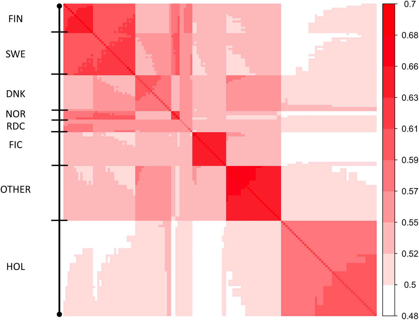
Heatmap of covariances between 148 MFs (Γ148). Diagonal of the heatmap plot are self-relationships of the MFs; off-diagonals are relationships between MFs.
Because Γ148 is an extrapolated matrix of Γpre we expect these to be alike. The difference between the two matrices was assessed using percentage deviation from the mean off-diagonal values in breed groups (Table 3). The average off-diagonal value of was 1.8% higher than in Γpre. For instance, the average relationships between the RDC FIN and FIC groups were 0.54 and 0.56 in Γpre and Γ148, respectively. Thus, the covariance function allows to extrapolate the Γ matrix for the MF approach in order to have the same number of MF as UPG.
TABLE 3
| FIN | SWE | DNK | NOR | RDC | FIC | OTHER | HOL | |
|---|---|---|---|---|---|---|---|---|
| FINa | 112.6b | 99.7 | 107.5 | 105.2 | 99.1 | 97.8 | 93.1 | |
| SWE | 110.1b | 100.8 | 109.6 | 104.2 | 97.8 | 97.4 | 93.2 | |
| DNK | 98.4 | 99.5 | 99.9 | 101.8 | 98.7 | 104.2 | 96.3 | |
| NOR | 106.4 | 108.6 | 97.6 | 102.3 | 98.0 | 96.8 | 92.9 | |
| RDC | 104.4 | 103.3 | 99.4 | 100.8 | 98.2 | 98.5 | 95.7 | |
| FIC | 97.8 | 96.3 | 95.8 | 95.7 | 95.8 | 99.7 | 92.0 | |
| OTHER | 96.3 | 95.9 | 101.3 | 94.5 | 96.0 | 96.8 | 93.6 | |
| HOL | 91.3 | 91.4 | 94.7 | 91.6 | 94.5 | 90.7 | 92.0 |
Deviation from average relationships between breed groups in Γpre (lower triangle) and Γ148 (upper triangle).
Deviation was computed as , where Γk,l is submatrix of Γ for breed groups k and l, and is off-diagonal submatrix of Γ
Groups were: FIN, Finnish Red Dairy Cattle; SWE, Swedish Red Dairy Cattle; DNK, Danish Red Dairy Cattle; NOR, Norwegian Red Dairy Cattle; RDC, Red Dairy Cattle from other countries; FIC, Finncattle; HOL, Finnish Holstein, and OTHER, breeds.
Application of the Γ148 matrix to the pedigree-based relationship matrix lifted the average diagonal elements of A22 closer to G05 (Figure 3). The smallest diagonal and off-diagonal values of A22 increased by 0.25 (from one to 1.25) and by 0.50 (from 0 to 0.50), respectively, by using as the basis for (Table 4). The increase was close to that in Kudinov et al. (2020) - 0.27 and 0.48 for the diagonal and off-diagonal elements, respectively. The correlations in the diagonal and off-diagonal elements were higher between G05 and (0.70 and 0.88) than between G05 and A22 (0.57 and 0.77). The overall magnitude of values in in our study was higher than presented for HOL in Koivula et al. (2022). Average relationship coefficients of A22, , and G05 in Koivula et al. (2022) had a steady increase by animal’s birth year. However, similar behavior in our study was observed only for the A22 matrix. A slight decrease in the average relationship coefficient of G05 and was observed after year 2000. This might be caused by the establishment of the joint Nordic RDC evaluation and admixture of the breads in the three populations. The total increase in the average relationships in the 40-year period were 2.81%, 0.97%, and 0.72% for A22, , and G05, respectively. The MF approach is beneficial in an admixed population such as Nordic RDC, as it helps to balance the G05 and A22 matrices. However, and G05 were not on exactly on the same scale as the mean diagonal and off-diagonal elements in were still somewhat lower than in G05 (Table 4). So, some compatibility issues between the pedigree- and genomic-based relationship matrices remained.
FIGURE 3
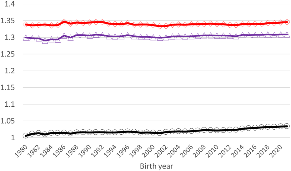
Average diagonal elements of A22 (black circles), AΓ (blue triangles), and G05 (red diamonds) by the birth year of a genotyped animal.
TABLE 4
| Elements | Matrix | Mean | Min | Max |
|---|---|---|---|---|
| Diagonal | A22 | 1.03 | 1.00 | 1.29 |
| 1.31 | 1.25 | 1.50 | ||
| G05 | 1.34 | 1.00 | 1.58 | |
| Off-diagonal | A22 | 0.06 | 0.00 | 0.82 |
| 0.61 | 0.50 | 1.17 | ||
| G05 | 0.68 | 0.47 | 1.40 |
Mean, minimum (Min), and maximum (Max) element values of A22, and G05 from diagonal and off-diagonal.
A22 - the pedigree relationship matrix of genotyped animals A22Γ - the pedigree relationship matrix of genotyped animals augmented by the G05 - the genomic relationship matrix with allele frequencies equal to 0.5.
In addition to Γpre, ΓRDC_HOL was tested as source for Γ148* and corresponding estimation. The mean difference between ΓRDC_HOL and Γpre was 0.03. Diagonal elements in constructed using extrapolated ΓRDC_HOL were on average 0.02 lower than in used for genomic prediction. Even though construction of Γpre with ΓRDC and ΓHOL diagonals helped to lift A22 closer to G05, this step was not vital and ΓRDC_HOL might have been used as it is.
Filtering of the SNPs by minor allele frequency (MAF) for the matrix estimation was elaborated in our previous study (Kudinov et al., 2020), and indirectly performed in Legarra et al. (2015). In the current study, we avoided MAF filtering of SNPs used to compute . That helped to compute a matrix closer to G05, as the same set of markers was used to construct G05. We observed that if selection of SNPs is used, it should be applied to both and G05, i.e., the same set of markers should be used consistently. It is reasonable to keep the set of markers used in G05 and as compatible as possible.
The presented approach in our study allows to fit the same number of MF as UPG and define MF for base population groups not linked to the genotypes. However, approach requires several arbitrary steps that need to be customized for each population. For instance, definition of the groups will be different in Γpre. We defined the groups in Γpre by breed, country, and time. If any of defined groups had less than 0.1% of genotyped animals, we have had to combine it. In our study, the definition of the time variable in the base populations used to compute AF was the last year of the time interval, another way is to use mean, median or the first year. Because the year definition in each of the groups is used in the model matrix Φ and resulting covariance function, average diagonal of would expectedly decrease. The standardized year of the MF in Φ was computed with the same formulae. However, this can be adjusted for specific breed or country. Use of a covariance function in routine genomic prediction need re-estimation of the Γ matrix when new genetic groups are defined, but not re-estimation of base AF.
3.2 Model runs and validation
The ssMF and ssUPG models converged in 1,388 and 2,802 iterations. The wall-clock time per iteration was similar for ssMF and ssUPG models. The mix99 runtime for ssMF model in Intel Xeon 2.8 Ghz machine with four cores was 11 h 19 min.
Table 5 presents bull validation results for the nine traits. For all traits, the highest prediction reliability was obtained by the ssMF model. The regression slopes () obtained by ssMF were slightly higher than by ssUPG. Prediction reliability by the pUPG and pMF models were the same. However, the slopes () with pMF were closer to one than with pUPG. In all traits and models, quality of prediction decreased from lactation one to 3. For the validation cows (Table 6), the ssMF model gave slightly better validation reliability in milk than the ssUPG model. For protein and fat, the same prediction reliability was estimated in both single-step models. The slope in ssMF was closer to one than in the other models. However, in the first parity milk trait, the slope was slightly above one in ssUPG and ssMF. The MF approach improved quality of genomic prediction in the studied population similarly as reported in Bradford et al. (2019), Masuda et al. (2021), and Koivula et al. (2022) The bias of prediction in the ssMF model was lower as reported for dairy sheep (Macedo et al., 2020). Nonetheless bias in our study remain significant in all single-step models.
TABLE 5
| Modela | ssUPG | ssMF | pUPG | pMF | |||||
|---|---|---|---|---|---|---|---|---|---|
| Trait - parity | Number of bulls | b1b | c | b1 | b1 | b1 | |||
| Milk 1 | 284 | 0.80 | 0.45 | 0.82 | 0.48 | 0.82 | 0.20 | 0.87 | 0.21 |
| Milk 2 | 243 | 0.77 | 0.37 | 0.81 | 0.39 | 0.89 | 0.22 | 0.93 | 0.22 |
| Milk 3 | 180 | 0.76 | 0.21 | 0.79 | 0.22 | 0.91 | 0.13 | 0.96 | 0.13 |
| Protein 1 | 287 | 0.64 | 0.34 | 0.66 | 0.36 | 0.54 | 0.11 | 0.59 | 0.11 |
| Protein 2 | 240 | 0.62 | 0.30 | 0.70 | 0.31 | 0.66 | 0.14 | 0.70 | 0.14 |
| Protein 3 | 181 | 0.66 | 0.18 | 0.68 | 0.19 | 0.74 | 0.10 | 0.80 | 0.10 |
| Fat 1 | 284 | 0.68 | 0.40 | 0.71 | 0.41 | 0.63 | 0.17 | 0.67 | 0.17 |
| Fat 2 | 241 | 0.73 | 0.39 | 0.78 | 0.40 | 0.70 | 0.16 | 0.73 | 0.16 |
| Fat 3 | 181 | 0.72 | 0.21 | 0.75 | 0.20 | 0.79 | 0.12 | 0.83 | 0.12 |
[G]EBV validation test regression coefficients (b1) and weighted validation reliabilities () for RDC validation bulls.
Models are: ssUPG, single-step GTBLUP, with UPG, accounted in H−1, ssMF, single-step GTBLUP, with MF; pUPG-pedigree BLUP, with UPG, accounted in A−1, and pMF, pedigree BLUP, with MF.
Regression coefficient b in equation has been multiplied by two.
Validation reliability was obtained from coefficient of determination of the model (Rmodel2), after correcting it by the average weight of DYDs ().
TABLE 6
| Modela | ssUPG | ssMF | pUPG | pMF | |||||
|---|---|---|---|---|---|---|---|---|---|
| Trait - parity | Number of cows | b1 | b | b1 | b1 | b1 | |||
| Milk 1 | 32,133 | 1.03 | 0.50 | 1.04 | 0.51 | 0.91 | 0.17 | 0.97 | 0.16 |
| Milk 2 | 27,097 | 0.96 | 0.41 | 0.97 | 0.42 | 0.93 | 0.15 | 0.98 | 0.15 |
| Milk 3 | 10,923 | 0.91 | 0.34 | 0.92 | 0.34 | 0.85 | 0.13 | 0.90 | 0.13 |
| Protein 1 | 33,298 | 0.87 | 0.36 | 0.89 | 0.36 | 0.80 | 0.14 | 0.84 | 0.14 |
| Protein 2 | 25,491 | 0.82 | 0.33 | 0.84 | 0.33 | 0.83 | 0.13 | 0.88 | 0.13 |
| Protein 3 | 10,387 | 0.83 | 0.29 | 0.84 | 0.29 | 0.78 | 0.11 | 0.83 | 0.11 |
| Fat 1 | 34,129 | 0.88 | 0.38 | 0.90 | 0.38 | 0.84 | 0.15 | 0.89 | 0.15 |
| Fat 2 | 25,987 | 0.83 | 0.32 | 0.85 | 0.32 | 0.85 | 0.14 | 0.90 | 0.14 |
| Fat 3 | 10,494 | 0.86 | 0.31 | 0.86 | 0.31 | 0.82 | 0.13 | 0.87 | 0.13 |
[G]EBV validation test regression coefficients (b1) and weighted validation reliabilities () for RDC validation cows.
Models are: ssUPG, single-step GTBLUP, with UPG, accounted in H−1, ssMF, single-step GTBLUP, with MF; pUPG-pedigree BLUP, with UPG, accounted in A−1, and pMF, pedigree BLUP, with MF.
Validation reliability was obtained from coefficient of determination of the model (Rmodel2), after correcting it by the average weight of DYDs ().
Genetic trends for combined milk, fat, and protein GEBVs are presented for the genotyped bulls with at least 50 daughters and all RDC cows in Figures 4, 5, respectively. Average GEBV were centered using the mean GEBV of RDC cows born in 2007. Both genomic and non-genomic models had similar shape in the UPG and MF instance. The average GEBV levels were higher than the average EBV levels. Similar difference has been observed in other single-step studies (Ma et al., 2015; Silva et al., 2019; Koivula et al., 2022). Overprediction in single-step with MF was reduced in our study similar to reported in Masuda et al. (2021) and Koivula et al. (2022).
FIGURE 4
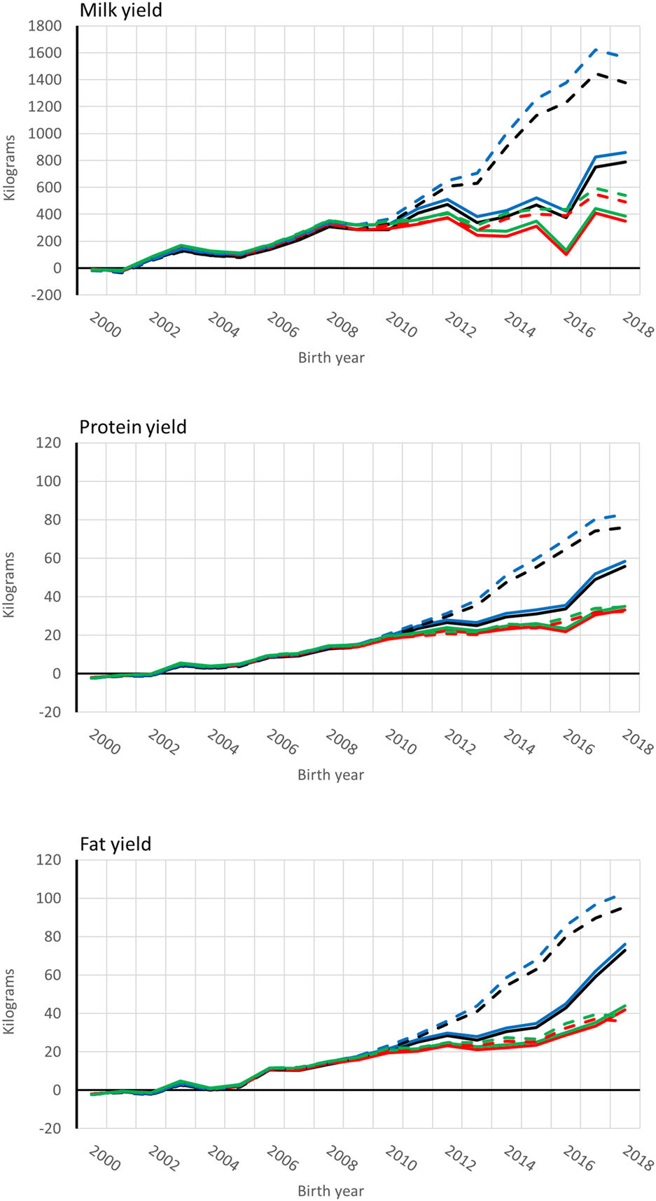
Average [genomic] breeding value of bulls by birth year in 305-d milk, protein, and fat yield (kg). Each bull had at least 50 daughters. Solid and dashed lines are from the model runs with full and reduced (minus four production year) data. Models are ssUPG—single-step GTBLUP with UPG accounted in H−1 (blue lines), ssMF—single-step GTBLUP with MF (black lines); pUPG-pedigree BLUP with UPG accounted in A−1 (green lines), and pMF—pedigree BLUP with MF (red lines).
FIGURE 5

Average [genomic] breeding value of cows by birth year in 305-d milk, protein, and fat yield (kg). Solid and dashed lines are from the model runs with full and reduced (minus four production year) data. Models are ssUPG—single-step GTBLUP with UPG accounted in H−1 (blue lines), ssMF—single-step GTBLUP with MF (black lines); pUPG-pedigree BLUP with UPG accounted in A−1 (green lines), and pMF—pedigree BLUP with MF (red lines).
Reduction of heritability by additive variance scaling was suggested by Legarra et al. (2015) when MF are used for genomic prediction. Base populations in models with UPGs are assumed unrelated, which is contrary to MF. In order to solve that problem additive variance was suggested to be scaled by , where tr(Γ) is the sum of diagonal elements of the Γ matrix (Legarra et al., 2015). However, this is based on assumption that the current population is a homogenous mixture of all the base populations that the MF will present. In reality base populations have influence unequally to the studied population, and thus we kept the same genetic variances in the UPG and MF models.
4 Conclusion
We presented a method to utilize the same number of MF as UPG in single-step GBLUP. The Covariance functions allowed smooth extrapolation of the matrix with 29 metafounders to 148 in the pedigree of all animals. Use of increased correlation between the elements of pedigree and genomic relationship matrices. The matrix was tested in the ssGTBLUP approach and compared with UPG based ssGTBLUP. Results showed a slight improvement in prediction reliability and overprediction in the MF model over the UPG model.
Statements
Data availability statement
The data analyzed in this study was obtained from Finncattle Foundation (Finland), Finnish Breeder Association (FABA, Finland), Swedish Cattle Farmers Association (Växa), Landbrug and Fødevarer F.m.b.A (L and F), Nordic Cattle Genetic Evaluation (NAV, Denmark), Viking Genetics (Denmark), and corresponding farmers. Requests to access these datasets should be directed to the Director of Nordic Cattle Genetic Evaluation, Gert P. Aamand, gap@lf.dk.
Author contributions
AK executed the analysis and wrote the manuscript. EM did the study design. MK, GA, IS, and EM provided support during analysis execution, reviewed, and edited the manuscript. All authors contributed to the article and approved the submitted version.
Funding
Project “Genomic evaluations for Western Finncattle” financed by Luke (Finland) and Finncattle Foundation (Finland).
Acknowledgments
We acknowledge Finncattle Foundation (Finland), Finnish Breeder Association (Finland), Nordic Cattle Genetic Evaluation (Denmark), and Viking Genetics (Denmark). We kindly acknowledge two reviewers participated in production of the current manuscript.
Conflict of interest
The authors declare that the research was conducted in the absence of any commercial or financial relationships that could be construed as a potential conflict of interest.
Publisher’s note
All claims expressed in this article are solely those of the authors and do not necessarily represent those of their affiliated organizations, or those of the publisher, the editors and the reviewers. Any product that may be evaluated in this article, or claim that may be made by its manufacturer, is not guaranteed or endorsed by the publisher.
References
1
AguilarI.MisztalI.JohnsonD. L.LegarraA.TsurutaS.LawlorT. J. (2010). Hot topic: A unified approach to utilize phenotypic, full pedigree, and genomic information for genetic evaluation of Holstein final score. J. Dairy Sci.93, 743–752. 10.3168/jds.2009-2730
2
BradfordH. L.MasudaY.VanRadenP. M.LegarraA.MisztalI. (2019). Modeling missing pedigree in single-step genomic BLUP. J. Dairy Sci.102, 2336–2346. 10.3168/jds.2018-15434
3
ChristensenO. F. (2012). Compatibility of pedigree-based and marker-based relationship matrices for single-step genetic evaluation. Genet. Sel. Evol.44, 37. 10.1186/1297-9686-44-37
4
ChristensenO. F.LundM. S. (2010). Genomic prediction when some animals are not genotyped. Genet. Sel. Evol.42, 2. 10.1186/1297-9686-42-2
5
Garcia-BaccinoC. A.LegarraA.ChristensenO. F.MisztalI.PocrnicI.VitezicaZ. G.et al (2017). Metafounders are related to Fst fixation indices and reduce bias in single-step genomic evaluations. Genet. Sel. Evol.49, 34. 10.1186/s12711-017-0309-2
6
Granado-TajadaI.LegarraA.UgarteE. (2020). Exploring the inclusion of genomic information and metafounders in Latxa dairy sheep genetic evaluations. J. Dairy Sci.103 (7), 6346–6353. 10.3168/jds.2019-18033
7
KirkpatrickM.LofsvoldD.BulmerM. (1990). Analysis of the inheritance, selection and evolution of growth trajectories. Genetics124 (4), 979–993. 10.1093/genetics/124.4.979
8
KluskaS.MasudaY.FerrazJ. B. S.TsurutaS.ElerJ. P.BaldiF.et al (2021). Metafounders may reduce bias in composite cattle genomic predictions. Front. Genet.12, 678587. 10.3389/fgene.2021.678587
9
KoivulaM.StrandénI.AamandG. P.MäntysaariE. A. (2022). Accounting for missing pedigree information with single-step random regression test-day models. Agriculture12, 388. 10.3390/agriculture12030388
10
KoivulaM.StrandénI.AamandG. P.MäntysaariE. A. (2021b). Meta-model for genomic relationships of metafoundersapplied on large scale single-step random regression test-day model. Interbull Bull.56, 76–81.
11
KoivulaM.StrandénI.AamandG. P.MäntysaariE. A. (2021a). Practical implementation of genetic groups in single-step genomic evaluations with Woodbury matrix identity-based genomic relationship inverse. J. Dairy Sci.104 (9), 10049–10058. 10.3168/jds.2020-19821
12
KudinovA. A.MäntysaariE. A.AamandG. P.UimariP.StrandénI. (2020). Metafounder approach for single-step genomic evaluations of Red Dairy cattle. J. Dairy Sci.103 (7), 6299–6310. 10.3168/jds.2019-17483
13
LegarraA.AguilarI.MisztalI. (2009). A relationship matrix including full pedigree and genomic information. J. Dairy Sci.92, 4656–4663. 10.3168/jds.2009-2061
14
LegarraA.ChristensenO. F.AguilarI.MisztalI. (2014). Single Step, a general approach for genomic selection. Livestock Sci.166, 54–65. 10.1016/j.livsci.2014.04.029
15
LegarraA.ChristensenO. F.VitezicaZ. G.AguilarI.MisztalI. (2015). Ancestral relationships using metafounders: Finite ancestral populations and across population relationships. Genetics200, 455–468. 10.1534/genetics.115.177014
16
LidauerM. H.PösöJ.PedersanJ.LassenJ.MadsenP.MäntysaariE. A.et al (2015). Across-country test-day model evaluations for Holstein, nordic red cattle, and Jersey. J. Dairy Sci.98, 1296–1309. 10.3168/jds.2014-8307
17
MaP.LundM. S.NielsenU. S.AamandG. P.SuG. (2015). Single-step genomic model improved reliability and reduced the bias of genomic predictions in Danish Jersey. J. Dairy Sci.98, 9026–9034. 10.3168/jds.2015-9703
18
MacedoF. L.ChristensenO. F.AstrucJ. M.AguilarI.MasudaY.LegarraA. (2020). Bias and accuracy of dairy sheep evaluations using BLUP and SSGBLUP with metafounders and unknown parent groups. Genet. Sel. Evol.52 (47), 47. 10.1186/s12711-020-00567-1
19
MäntysaariE. A.LiuZ.VanRadenP. M. (2010). Interbull Bulletin41, 17–22.
20
MäntysaariE. A.KoivulaM.StrandénI. (2020). Symposium review: Single-step genomic evaluations in dairy cattle. J. Dairy Sci.103 (6), 5314–5326. 10.3168/jds.2019-17754
21
MäntysaariE. A.EvansR.StrandénI. (2017). Efficient single-step genomic evaluation for a multibreed beef cattle population having many genotyped animals. J. Anim. Sci.95, 4728–4737. 10.2527/jas2017.1912
22
MasudaY.TsurutaS.BermannM.BradfordH. L.MisztalI. (2021). Comparison of models for missing pedigree in single-step genomic prediction. J. Anim. Sci.99 (2), skab019. 10.1093/jas/skab019
23
MasudaY.VanRadenP. M.ShogoT.LourencoD. A. L.MisztalI. (2022). Invited review: Unknown-parent groups and metafounders in single-step genomic BLUP. J. Dairy Sci.105 (2), 923–939. 10.3168/jds.2021-20293
24
MatilainenK.StrandénI.AamandG. P.MäntysaariE. A. (2018). Single step genomic evaluation for female fertility in Nordic Red dairy cattle. J. Anim. Breed. Genet.135, 337–348. 10.1111/jbg.12353
25
McPeekM. S.XiaodongW.OberC. (2004). Best linear unbiased allele-frequency estimation in complex pedigrees. Biometrics60, 359–367. 10.1111/j.0006-341X.2004.00180.x
26
MisztalI.LourencoD. A. L.LegarraA. L. (2020). Current status of genomic evaluation. J. Anim. Sci.98, skaa101. 10.1093/jas/skaa101
27
MisztalI.VitezicaZ. G.LegarraA.AguilarI.SwanA. A. (2013). Unknown‐parent groups in single‐step genomic evaluation. J. Anim. Breed. Genet.130, 252–258. 10.1111/jbg.12025
28
PatryC.DucrocqV. (2011). Evidence of biases in genetic evaluations due to genomic preselection in dairy cattle. J. Dairy Sci.94, 1011–1020. 10.3168/jds.2010-3804
29
PoulsenB. G.OstersenT.NielsenB.ChristensenO. F. (2022). Predictive performances of animal models using different multibreed relationship matrices in systems with rotational crossbreeding. Genet. Sel. Evol.54 (1), 25–17. 10.1186/s12711-022-00714-w
30
PřibylJ.MadsenP.BauerJ.PřibylováJ.ŠimečkováM.VostrýL.et al (2013). Contribution of domestic production records, Interbull estimated breeding values, and single nucleotide polymorphism genetic markers to the single-step genomic evaluation of milk production. J. Dairy Sci.96 (3), 1865–1873. 10.3168/jds.2012-6157
31
QuaasR. L.PollakE. J. (1981). Modified equations for sire models with groups. J. Dairy Sci.64, 1868–1872. 10.3168/jds.S0022-0302(81)82778-6
32
SilvaA. A.SilvaD. A.SilvaF. F.CostaC. N.LopesP. S.CaetanoA. R.et al (2019). Autoregressive single-step test-day model for genomic evaluations of Portuguese Holstein cattle. J. Dairy Sci.102 (7), 6330–6339. 10.3168/jds.2018-15191
33
StrandénI.LidauerM. (1999). Solving large mixed linear models using preconditioned conjugate gradient iteration. J. Dairy Sci.82, 2779–2787. 10.3168/jds.S0022-0302(99)75535-9
34
StrandénI.MäntysaariE. A. (2020). Bpop: An efficient program for estimating base population allele frequencies in single and multiple group structured populations. AFSci.29 (3), 166–176. 10.23986/afsci.90955
35
StrandénI.VuoriK. (2006). “RelaX2: Pedigree analysis program,” in Proceedings of the 8th World Congress on Genetics Applied to Livestock Production, 13-18 August 2006 (Belo Horizonte, MG, Brazil: Instituto Prociência), 27–30.
36
TaskinenM.MäntysaariE. A.AamandG. P.StrandénI. (2014). “Comparison of breeding values from single-step and bivariate blending methods,” in Proceedings of the 10th World Congress on Genetics Applied to Livestock Production, August 2014 (Vancouver, BC, Canada: WCGALP), 17–22.
37
TijaniA.WiggansG. R.Van TassellC. P.PhilpotJ. C.GenglerN. (1999). Use of (co) variance functions to describe (co)variances for test day yield. J. Dairy Sci.82 (1), 22610–22614. 10.3168/jds.S0022-0302(99)75228-8
38
VanRadenP. M. (2008). Efficient methods to compute genomic predictions. J. Dairy Sci.91, 4414–4423. 10.3168/jds.2007-0980
39
VitezicaZ. G.AguilarI.MisztalI.LegarraA. (2011). Bias in genomic predictions for populations under selection. Genet. Res.93, 357–366. 10.1017/S001667231100022X
40
WiggansG. R.ColeJ. B.HubbardS. M.SonstegardT. S. (2017). Genomic selection in dairy cattle: The USDA experience. Annu. Rev. Anim. Biosci.5 (1), 309–327. 10.1146/annurev-animal-021815-111422
41
WiggansG. R.VanRadenP. M.CooperT. A. (2011). The genomic evaluation system in the United States: Past, present, future. J. Dairy Sci.94 (6), 3202–3211. 10.3168/jds.2010-3866
42
XiangT.ChristensenO. F.LegarraA. (2017). Technical note: Genomic evaluation for crossbred performance in a single-step approach with metafounders. J. Anim. Sci95, 1472–1480. 10.2527/jas.2016.1155
Appendix 1: Representation of the Φpre matrix used in formula to compute the K matrix.
1 STY - birth year of the group standardized as , where yearMF is the year of the MF, yearmin = 1950 and yearmax = 2021.
Summary
Keywords
genetic groups, genomic evaluation, red dairy cattle, finncattle, co-variance function
Citation
Kudinov AA, Koivula M, Aamand GP, Strandén I and Mäntysaari EA (2022) Single-step genomic BLUP with many metafounders. Front. Genet. 13:1012205. doi: 10.3389/fgene.2022.1012205
Received
05 August 2022
Accepted
31 October 2022
Published
21 November 2022
Volume
13 - 2022
Edited by
Martino Cassandro, University of Padua, Italy
Reviewed by
Andres Legarra, INRAE Occitanie Toulouse, France
Ivan Pocrnić, University of Edinburgh, United Kingdom
Updates
Copyright
© 2022 Kudinov, Koivula, Aamand, Strandén and Mäntysaari.
This is an open-access article distributed under the terms of the Creative Commons Attribution License (CC BY). The use, distribution or reproduction in other forums is permitted, provided the original author(s) and the copyright owner(s) are credited and that the original publication in this journal is cited, in accordance with accepted academic practice. No use, distribution or reproduction is permitted which does not comply with these terms.
*Correspondence: Andrei A. Kudinov, andrei.kudinov@luke.fi
This article was submitted to Livestock Genomics, a section of the journal Frontiers in Genetics
Disclaimer
All claims expressed in this article are solely those of the authors and do not necessarily represent those of their affiliated organizations, or those of the publisher, the editors and the reviewers. Any product that may be evaluated in this article or claim that may be made by its manufacturer is not guaranteed or endorsed by the publisher.