Estimating heritability of complex traits from genome-wide association studies using IBS-based Haseman–Elston regression

Exploring heritability of complex traits is a central focus of statistical genetics. Among various previously proposed methods to estimate heritability, variance component methods are advantageous when estimating heritability using markers. Due to the high-dimensional nature of data obtained from genome-wide association studies (GWAS) in which genetic architecture is often unknown, the most appropriate heritability estimator model is often unclear. The Haseman–Elston (HE) regression is a variance component method that was initially only proposed for linkage studies. However, this study presents a theoretical basis for a modified HE that models linkage disequilibrium for a quantitative trait, and consequently can be used for GWAS. After replacing identical by descent (IBD) scores with identity by state (IBS) scores, we applied the IBS-based HE regression to single-marker association studies (scenario I) and estimated the variance component using multiple markers (scenario II). In scenario II, we discuss the circumstances in which the HE regression and the mixed linear model are equivalent; the disparity between these two methods is observed when a covariance component exists for the additive variance. When we extended the IBS-based HE regression to case-control studies in a subsequent simulation study, we found that it provided a nearly unbiased estimate of heritability, more precise than that estimated via the mixed linear model. Thus, for the case-control scenario, the HE regression is preferable. GEnetic Analysis Repository (GEAR; http://sourceforge.net/p/gbchen/wiki/GEAR/) software implemented the HE regression method and is freely available.

Introduction

So-called “missing heritability” can occur due to various reasons, such as small sample size, underrepresented variant spectrum, experimental design, and improper methodological assumptions (Manolio et al., 2009). Because of the high-dimensional nature of genome-wide association study (GWAS) data, in which the number of markers (M) is far greater than the number of individuals (N), estimating heritability is difficult. For instance, if the statistical power is insufficient, variants associated with a small effect may not be captured under a stringent p-value threshold (~ 10⁻⁸). This obstacle can be partially bypassed by implementing the mixed linear model, which uses the genetic relationship between individuals estimated from single nucleotide polymorphism (SNP) markers in lieu of fitting hundreds of thousands of markers together (Yang et al., 2010). Nevertheless, it has been recently disputed how an estimator should be adjusted under genetic architecture. Speed et al. (2012) suggested using a weighted genetic relationship matrix under different genetic architecture, which is often unknown. As demonstrated in large-scale empirical data studies (Lee et al., 2013), Speed's ad-hoc weighing method depends on the genetic architecture and does not often outperform plain weight methods upon comparison. As the genetic architecture, such as the relationship between variant frequency and variant effect, is often unknown, criteria should be established to justify the model used to estimate heritability.

For GWAS, as many samples are collected to study diseases, many studies eventually adopt a case-control design. Due to ascertainment in case-control studies, scale transformation is necessary. Without scale transformation, the heritability on the observed scale can be greater than 1, rendering the estimated heritability meaningless, as it is not representative of its heritability on the liability scale, which is more interpretable (Falconer, 1966) for disease data. An equation (Lee et al., 2011) that transforms heritability from the observed scale to the liability scale has been proposed (as the equation was indexed as the 23rd equation in Sang Hong Lee's paper, it is henceforth denoted as Hong23) and was investigated under the infinitesimal model, for which the number of casual loci is infinite. However, in practice, disease loci are reasonably limited for many diseases (Yang et al., 2011), which raises the question of whether or not Hong23 works well for mixed linear model estimates if the infinitesimal model does not hold.

All of the above concerns are related to the heritability estimated via variance component methods implemented thus far in mixed linear models. The Haseman–Elston (HE) regression is a prestigious method for estimating variance components (Haseman and Elston, 1972). The HE regression, a well-known tool for linkage studies that uses identity by descent (IBD) (Lynch and Walsh, 1998; Hill and Weir, 2011) scores, however, seems a rusty weapon in the genomics analysis armory of the GWAS era. This is because the HE regression relies on relatedness measured on IBD but not identity by state (IBS). Although IBS has been employed for linkage analysis, such as under affected-pedigree-member design (Lange, 1986b; Weeks and Lange, 1988; Bishop and Williamson, 1990), its performance is largely dependent on marker polymorphisms and may cause high false positives when ad-hoc weighting functions or incorrect frequencies are adopted. As an underrepresented concept of the linkage era, IBS is neither well-adapted to linkage studies nor employed in the original HE regression framework.

Taken together, the following questions remain.

(1) Can the HE regression be applied to the IBS content such as for GWAS? If the answer is affirmative, what is the theoretical basis and the genetic interpretation in this new context?

(2) An equilibrium has been established between the HE regression and the variance component method (Sham et al., 2002) for linkage studies. Does this equilibrium stand for high-dimensional data such as GWAS data and what are its assumptions?

(3) If the IBS-based HE regression is applied to case-control studies, can it estimate heritability better than the mixed linear models?

(4) Given the recent dispute regarding heritability estimation of complex traits, can HE regression provide further justification?

Recently, a new theory using like-standardized IBS has paved another route to assess genetic relatedness (Ritland, 1996; Powell et al., 2010; Yang et al., 2010) between unrelated individuals (conventional sense). The IBS score resembles the conventional IBD score (Powell et al., 2010), which raises the question of whether this IBS score can be used in the HE regression for unrelated individuals. In this study, by replacing the IBD scores with standardized IBS scores, we used the HE regression to conduct association studies for GWAS data. Assuming random mating, biallelic loci, and additive genetic effects only on the genetic architecture of quantitative trait loci (QTLs) underlying a complex trait, this report establishes the theoretical basis for using the HE regression for GWAS. Two generic scenarios were investigated, and their regression coefficients were derived and have genetically meaningful interpretations. In scenario I, the IBS score was assessed via a marker that was in linkage disequilibrium (LD) with a QTL. This enabled the HE regression to be a tool for single-marker GWAS. In scenario II, IBS score was assessed on multiple markers, each of which could be in LD with multiple QTLs. This allowed the HE regression to be used to estimate the variance component tagged by markers.

The second scenario has implications for estimation of heritability for complex trait using whole genome-wide markers together, similar to the mixed linear model (Yang et al., 2010; Lee et al., 2011). Using an analytical method that establishes the equivalence between the IBS-based HE regression and the mixed linear model, a simple criterion is proposed to justify the estimates in this study. A similar equivalence between the HE regression and the variance component analysis with the mixed linear model was determined in the context of linkage analysis (Sham and Purcell, 2001). In this study, their equivalence is established under the context of GWAS, and the conditions for equivalence are explored analytically as well as in silico. After extending the established HE regression into case-control scenarios, we demonstrated that Hong23 fits the estimate from the HE regression better than that from the mixed linear model.

Furthermore, as the IBS-based HE regression uses least squares, it is advantageous in its computational efficiency and is N (N is the sample size) times faster than the mixed linear model. In order to facilitate the application, the HE regression algorithm for GWAS data was implemented in Java software, GEnetic Analysis Repository (GEAR), which is freely available online.

As the first half of this report is focused on establishing the mathematical basis of the IBS-based HE regression, many mathematical symbols are introduced (Table 1). In the text below, the HE regression is the IBS-based HE regression unless explicitly noted otherwise.

TABLE 1

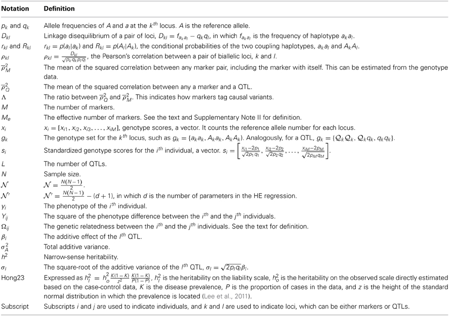
Table 1. Notation definitions.

Theory of the IBS-Based HE Regression

For an individual, the phenotype is denoted as y_i, which follows the normal distribution of N(μ_y, σ²_y), and the genotype is x_i = [x_i1, x_i2, …, x_iM], in which M is the number of markers. For the i^th individual, the genotype at the k^th locus is x_ik, which counts the reference alleles at the k^th locus. The reference allele is denoted as A_k and the alternative is a_k. The frequency of A_k is p_k and the frequency of a_k is q_k. g_k is the set of possible genotypes, say {a_ka_k, A_ka_k, A_kA_k}, at the k^th locus. Consequently, a_ka_k, A_ka_k, and A_kA_k are coded as 0, 1, and 2, respectively. After standardization, x_i is expressed as $s_i=\left[\frac{x_{i1}-2p_1}{\sqrt{2p_1{q}_1}},\frac{x_{i2}-2p_2}{\sqrt{2p_2{q}_2}},\dots ,\frac{x_{iM}-2p_M}{\sqrt{2p_M{q}_M}}\right]$. For x_ik, given a genotype of a_ka_k, A_ka_k, and A_kA_k, their standardized scores are $\frac{-2p_k}{\sqrt{2p_k{q}_k}},\frac{q_k-p_k}{\sqrt{2p_k{q}_k}}$, and $\frac{2q_k}{\sqrt{2p_k{q}_k}}$, respectively. The additive effect of the l^th QTL is denoted as β_l. Throughout the study, we assume a polygenic model with L QTLs.

The IBS-Based HE Regression

Haseman and Elston (1972) proposed a linear model, Y_ij = μ + bπ_ij + e_ij, for detecting linkage between a marker and a QTL in a full-sib design. Y_ij represents the squared difference between a pair of full sibs, and π_ij is the proportion of IBD at an observed marker locus; μ is the intercept of the regression, b is the regression coefficient, and e_ij is the residual. The mathematical expectation of the regression coefficient is b = −2(1 − 2c)² σ²_A, in which c is the recombination fraction between the marker locus and the QTL, and σ²_A is the additive genetic variance of the QTL.

Now consider a sample consisting of N unrelated individuals. If the phenotype for the i^th individual is y_i, we can modify the HE original regression as below

$\begin{array}{cc}{Y}_{ij}=\mu +b{\Omega }_{ij}+e_{ij}& (1)\end{array}$

in which Y_ij = (y_i − y_j)² represents the squared difference, Ω_ij is the measure of the genetic relatedness of a pair of individuals, and e_ij is the residual. Given N unrelated individuals, there are such individual pairs. Ω_ij is the similarity score between a pair of individuals based on the IBS, as recently proposed (Powell et al., 2010; Yang et al., 2010).

For the linear model in Equation (1), the expectation of the regression coefficient is $E(b)=\frac{cov(Y_{ij},{\Omega }_{ij})}{var({\Omega }_{ij})}$. var(Ω_ij) is the variance of the genetic relatedness. cov(Y_ij, Ω_ij) = E(Ω_ijY_ij) − E(Ω_ij)E(Y_ij) = E(Ω_ijY_ij) because E(Ω_ij) = 0 [see the definition for Ω_ij in section The Derivation of var(Ω_ij) and Effective Number of Markers (M_e)], and $E\left({\Omega }_{ij}{Y}_{ij}\right)={\Sigma }_{k=1}^M{\Sigma }_{x_{ik}\in g_k}{\Sigma }_{x_{jk}\in g_k}{s}_{ik}{s}_{jk}{\left[E\left(y_i|x_{ik}\right)-E\left(y_j|x_{jk}\right)\right]}^{2}p\left(x_{ik}\right)p(x_{jk})$ is the mathematical expectation of the joint distribution for Ω_ij and Y_ij. In order to derive var(Ω_ij) and cov(Y_ij, Ω_ij), we need to introduce the haplotype distribution of a biallelic loci pair (section Haplotypes of a Biallelic Loci Pair). When the haplotype is constructed on a pair of markers, it leads to the derivation of var(Ω_ij) [section The Derivation of var(Ω_ij) and Effective Number of Markers (M_e)]; when the haplotype is constructed for a marker and a QTL, it leads to E(y_i|x_ik), the conditional expectation of the phenotype based on a marker [section The Derivation of E(y_i|x_ik)].

Derivations of var(Ω_ij) and E(y_i|x_ik)

Haplotypes of a biallelic loci pair

For a pair of biallelic loci, there are four haplotype phases, and their conditional probabilities are as summarized in Table S1. r_kl = p(a_l|a_k) and R_kl = p(A_l|A_k) are defined as the conditional probabilities of the haplotypes in the coupling phases, such as a_ka_l and A_kA_l, respectively; 1 − r_kl and 1 − R_kl represent the conditional probabilities of the alleles in their repulsion phases, such as a_kA_l and A_ka_l, respectively. D_kl = f_AkAl − p_kp_l, in which f_AkAl is the frequency of the haplotype A_kA_l; D_kl is the covariance between the loci, quantifying the LD between them.

The correlation of a pair of biallelic loci can be expressed as a 2 × 2 correlation

$\begin{array}{cc}{\rho }_{kl}=\frac{D_{kl}}{\sqrt{p_k{q}_k{p}_l{q}_l}}& (2)\end{array}$

ρ²_kl is often used to parameterize the LD of a loci pair (Hill and Robertson, 1968). For more LD parameterization, please refer to Devlin and Risch (1995) and Wray (2005).

Once the conditional probabilities of the haplotypes are defined, it is straightforward to obtain the joint probabilities of the genotypes for a pair of loci. For example, under random mating, the probability of the genotype A_kA_kA_lA_l is p(A_kA_kA_lA_l) = p(A_kA_k|A_lA_l)p(A_kA_k) = p(A_l|A_k)p(A_k) p(A_l|A_k)p(A_k) = p²_kR²_kl. Analogously, this leads to the joint probabilities of the other eight two-locus genotypes (See Table 2).

TABLE 2

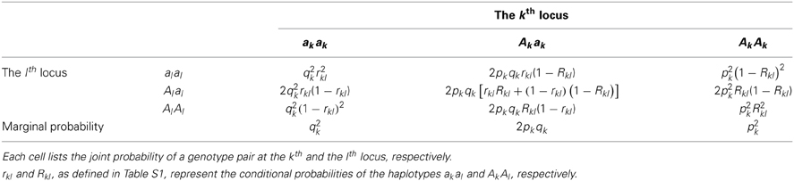
Table 2. The joint distribution of two loci.

The derivation of var(Ω_ij) and effective number of markers (M_e)

For a sample consisting of unrelated individuals, their pairwise genetic relationships, say additive genetic relationships, can be estimated with genetic markers, such as SNP markers (Powell et al., 2010; Yang et al., 2010). The genetic relatedness Ω_ij between the i^th individual and the j^th individual is measured by the dot product of their standardized genotypes and then divided by the number of markers.

$\begin{array}{cc}{\Omega }_{ij}=\frac{s_i.s_j}{M}=\frac{1}{M}{\Sigma }_{k=1}^M\frac{(x_{ik}-2p_k)}{\sqrt{2p_k{q}_k}}\frac{(x_{jk}-2p_k)}{\sqrt{2p_k{q}_k}}& (3)\end{array}$

The possible relatedness scores of a pair of individuals are summarized in Table 3A, totaling nine products. After combining the same score values, there are seven unique terms as in Table 3B. It is easy to derive that E(Ω_ij) = 0 and $var\left({\Omega }_{ij}\text{}\right)=\frac{1}{M^2}{\Sigma }_{k=1}^M{\Sigma }_{l=1}^{M}cov\left({\Omega }_{ijk},{\Omega }_{ijl}\right)$, in which cov(Ω_ijk, Ω_ijl) = E(Ω_ijkΩ_ijl) − E(Ω_ijk)E(Ω_ijk) = E(Ω_ijkΩ_ijl) because E(Ω_ij.) = 0.

TABLE 3A

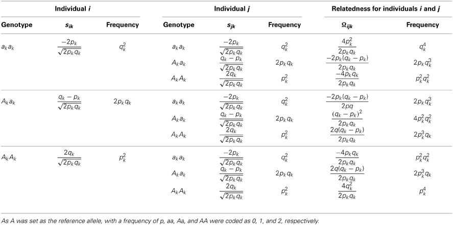
Table 3A. The joint distribution of the genetic relatedness between individuals i and j.

TABLE 3B

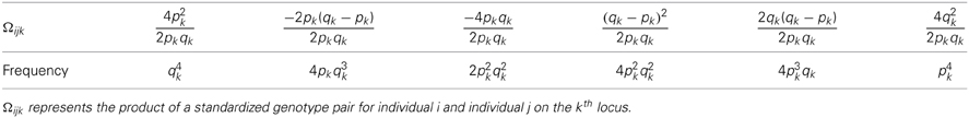
Table 3B. A reorganization of Table 3A to illustrate the relatedness joint distribution of a pair of individuals.

Ω_ij is informative in revealing hidden relatedness. For example, for the duplicated individual in the sample, E(Ω_ij) = 1; for first-degree relatives, E(Ω_ij) = 0.5; for second-degree relatives, E(Ω_ij) = 0.25. Consequently, it can control the entry of samples that are under the expected cutoff for relatedness.

After some additional algebra (see Supplementary Note I), we arrived at the following equation.

$\begin{array}{cc}cov\left({\Omega }_{ijk},{\Omega }_{ijl}\right)={\rho }_{kl}^2& (4)\end{array}$

When the k^th locus and the l^th locus are in linkage equilibrium, cov(Ω_ijk, Ω_ijl) = 0; when the k^th locus and the l^th locus are at the same locus, cov(Ω_ijk, Ω_ijl) = 1.

$\begin{array}{cc}var\left({\Omega }_{ij}\right)=\frac{1}{M^2}{\Sigma }_{k=1}^M{\Sigma }_{l=1}^M{\rho }_{kl}^2=\frac{1}{M}+\frac{1}{M^2}{\Sigma }_{k=1}^M{\Sigma }_{l\ne k}^M{\rho }_{kl}^2& (5)\end{array}$

The distribution of ρ²_kl varies with p_k and p_l (Wray, 2005). We can also interpret var(Ω_ij) as the mean of the squared Pearson's correlation between the markers along the genome, denoted as ρ²_M.

For simplicity of the following derivation, the concept of an effective number of markers, M_e, is introduced here. Intuitively, as markers are often in linkage disequilibrium, the real number of “independent” markers is smaller than the total number of the markers genotyped. This concept was previously introduced under the context of risk prediction (Purcell et al., 2009), and M_e was evaluated using Monte Carlo simulation. As indicated in Supplementary Note II, 1/var(Ω_ij) is the mathematical expectation of the effective number of markers evaluated under the simulation method (Purcell et al., 2009). For example, for 100 equifrequent biallelic loci, if the correlation for each pair of consecutive markers is 0, 0.25, 0.5, and 0.75, the effective number of markers is approximately 100, 90, 61, and 29, respectively. Real GWAS data are often at a magnitude of 10⁴ (Vinkhuyzen et al., 2013).

The derivation of E(y_i|x_ik)

The expected phenotype of y_i given genotype x_ik depends on the QTL genotype, say the l^th locus, in LD with x_ik. Assuming a biallelic QTL in LD with the marker, the conditional expectation of the marker is E(y_i|x_ik = A_kA_k) = Σ_xilgls_ilp(x_il|x_ik = A_kA_k), in which g_l = {_{l l}, _lq_l, q_lq_l}, and E(y_i|x_ik = A_kA_k) = β_l × R_kl² + 0 × 2R_kl (1 − R_kl) − β_l × (1 − R_kl)² = (2R_kl − 1)β_l. Analogously, we can derive the expected values of E(y_i|x_ik = A_ka_k) = (R_kl − r_kl)β_l and E(y_i|x_ik = a_ka_k) = (1 − 2r_kl)β_l (See Table 4). Once E(y_i|x_ik) is defined, the distribution of E(Y_ij|x_ik, x_jk) can be tabulated as in Table 5.

TABLE 4

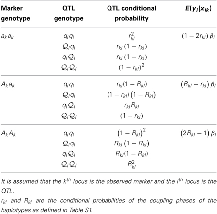
Table 4. The expected phenotype conditional to one's genotype on the observed marker.

TABLE 5

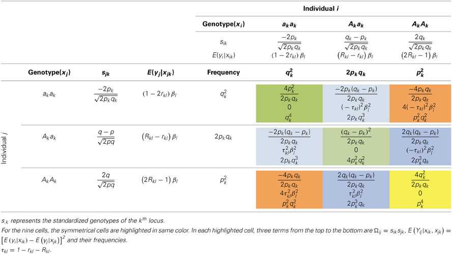
Table 5. The joint distribution of E(Ω_ij) and E(Y_ij|x_i, x_j) for one marker and one QTL.

Deriving the Mathematical Expectation of the Regression Coefficient

In this section, we investigated two scenarios to derive the expected value of the regression coefficient for Equation (1). In scenario I, genetic similarity is estimated at a single marker, which is in LD with one or more QTLs. In scenario II, genetic similarity is estimated based on M markers, each of which can be in LD with L QTLs.

Scenario I: one marker and one QTL

Under the scenario of one marker, say the k^th marker, and one QTL, say the l^th QTL, since var(Ω_ijk) = 1, E(b) = E(Ω_ijY_ij), which is E(Ω_ijY_ij) = Σ_xikΣ_xjks_iks_jk[E(y_i|x_ik) − E(y_j|x_jk)]²p(x_ik)p(x_jk). Consequently, we can derive the regression coefficient as

$\begin{array}{l}E\left(b\right)=E\left({\Omega }_{ij}{Y}_{ij}\right)={\Sigma }_{x_{ik}}{\Sigma }_{x_{jk}}{s}_{ik}{s}_{jk}[E\left(y_i|x_{ik}\right)\hfill \\ {-E\left(y_j|x_{jk}\right)]}^{2}p\left(x_{ik}\right)p(x_{jk})=\frac{-2p_k\left(q_k-p_k\right)}{2p_k{q}_k}{\tau }_{kl}^2{\beta }_l^{2}2p_k{q}_k^3\hfill \\ +\frac{-2p_k\left(q_k-p_k\right)}{2p_k{q}_k}{\left(-{\tau }_{kl}\right)}^2{\beta }_l^{2}2p_k{q}_k^3+\frac{-4p_k{q}_k}{2p_k{q}_k}4{\tau }_{kl}^2{\beta }_l^2{p}_k^2{q}_k^2\hfill \\ +\frac{-4p_k{q}_k}{2p_k{q}_k}4{\left(-{\tau }_{kl}\right)}^2{\beta }_l^2{p}_k^2{q}_k^2+\frac{2q_k\left(q_k-p_k\right)}{2p_k{q}_k}{\tau }_{kl}^2{\beta }_l^{2}2p_k^3{q}_k\hfill \\ +\frac{2q_k\left(q_k-p_k\right)}{2p_k{q}_k}{\left(-{\tau }_{kl}\right)}^2{\beta }_l^{2}2p_k^3{q}_k\hfill \end{array}$

and

$\begin{array}{cc}E(b)=-4{\tau }_{kl}^2{p}_k{q}_k{\beta }_l^2& (6)\end{array}$

in which τ_kl = 1 − r_kl − R_kl.

When the QTL overlaps with the marker, or the correlation between the QTL and the marker is 1, E(b) = −4p_kq_k β²_l because r_kl = R_kl = 1. When the QTL is in linkage equilibrium with the marker, r_kl = q_l and R_kl = p_l, 1 − r_kl − R_kl = 0, and consequently E(b) = 0.

According to Table S1, $r_{kl}+R_{kl}=\left(q_l+\frac{D_{kl}}{q_k}\right)+\left(p_l+\frac{D_{kl}}{p_k}\right)=1+\frac{D_{kl}}{p_k{q}_k}$. Consequently, the expression of Equation (6) can be rearranged as $E(b)=-4{\left(\frac{D_{kl}}{p_k{q}_k}\right)}^2{p}_k{q}_k{\beta }_l^2$. The correlation of a pair of biallelic loci ${\rho }_{kl}=\frac{D_{kl}}{\sqrt{p_k{q}_k{p}_l{q}_l}}$ [Equation (2)], and consequently E(b) = − 2ρ²_klσ²_l, in which ${\sigma }_l=\sqrt{2p_l{q}_l}{\beta }_l$. Alternatively, we can write

$\begin{array}{cc}E(b)=-2{\rho }_{kl}^2{\sigma }_l^2.& (7)\end{array}$

In the GWAS context, squared LD (Pearson's correlation) is in lieu of the recombination fraction for linkage. The mathematical expectation of the regression coefficient resembles the one in the original HE regression. However, it should be noted that here the interpretation of the regression coefficient is based on linkage disequilibrium and association, whereas the original interpretation is based on linkage between the marker and the QTL.

When multiple QTLs are in LD with the marker, the conditional expectation for y_i given x_ik is $E\left(y_i|x_{ik}=A_k{A}_k\right)={\Sigma }_l^L(2R_{kl}-1){\beta }_l,E\left(y_i|x_{ik}=A_k{a}_k\right)={\Sigma }_l^L(R_{kl}-r_{kl}){\beta }_l$, and $E\left(y_i|x_{ik}=a_k{a}_k\right)={\Sigma }_l^L(1-2r_{kl}){\beta }_l$, respectively. The joint distribution of Ω_ij and Y_ij is as summarized in Table S2, which resembles Table 5. Still using E(Ω_ijY_ij) = Σ_xikΣ_xjks_iks_jk[E(y_i|x_ik) − E(y_j|x_jk)]²p(x_ik)p(x_jk), the regression coefficient can be derived as below.

$\begin{array}{cc}\begin{array}{l}E(b)=\frac{-2p_k\left(q_k-p_k\right)}{2p_k{q}_k}{\left[{\Sigma }_{l=1}^L{\tau }_{kl}{\beta }_l\right]}^{2}2p_k{q}_k^3\hfill \\ +\frac{-4p_k{q}_k}{2p_k{q}_k}4{\left[{\Sigma }_{l=1}^L{\tau }_{kl}{\beta }_l\right]}^2{p}_k^2{q}_k^2\hfill \\ +\frac{2q_k\left(q_k-p_k\right)}{2p_k{q}_k}{\left[{\Sigma }_{l=1}^L{\tau }_{kl}{\beta }_l\right]}^{2}2p_k^3{q}_k\hfill \\ +\frac{-2p_k\left(q_k-p_k\right)}{2p_k{q}_k}{\left[{\Sigma }_{l=1}^L-{\tau }_{kl}{\beta }_l\right]}^{2}2p_k{q}_k^3\hfill \\ +\frac{-4p_k{q}_k}{2p_k{q}_k}4\left[{\Sigma }_{l=1}^L-{\tau }_{kl}{\beta }_l\right]p_k^2{q}_k^2\hfill \\ +\frac{2q_k\left(q_k-p_k\right)}{2p_k{q}_k}{\left[{\Sigma }_{l=1}^L-{\tau }_{kl}{\beta }_l\right]}^{2}2p_k^3{q}_k\hfill \\ =-4p_k{q}_k{\left[{\Sigma }_{l=1}^L{\tau }_{kl}{\beta }_l\right]}^2\hfill \end{array}& (8)\end{array}$

Equation (8) can be rearranged as

$\begin{array}{cc}E\left(b\right)=-2{\Sigma }_{l_1=1}^L{\Sigma }_{l_2=1}^L{\rho }_{k{l}_1}{\rho }_{k{l}_2}{\sigma }_{l_1}{\sigma }_{l_2}.& (9)\end{array}$

It is easy to see that when L = 1, Equation (9) can be simplified to Equation (7).

Scenario II: multiple markers and multiple QTLs

When the genetic relatedness matrix is constructed with M markers, each of which may be in LD with L QTLs, the HE regression becomes Y_ij = a + bΩ_ij, in which ${\Omega }_{ij}=\frac{1}{M}{\Sigma }_k^M{s}_{ik}{s}_{jk}$. For convenience, Ω_ijk denotes the relatedness fraction constructed with the k^th marker between the i^th and the j^th individuals. According to the definition of the regression coefficient, $b=\frac{Cov({\Omega }_{ij},Y_{ij})}{var({\Omega }_{ij})}$.

$\begin{array}{l}cov({\Omega }_{ij},Y_{ij})=\frac{1}{M}cov({\displaystyle \sum _{k=1}^M{\Omega }_{ijk}},Y_{ij})=\frac{1}{M}{\displaystyle \sum _{k=1}^{M}cov}({\Omega }_{ijk},Y_{ij})\hfill \\ =\frac{1}{M}{\displaystyle \sum _{k=1}^M-}4p_k{q}_k{[{\Sigma }_{l=1}^L{\tau }_{kl}{\beta }_l]}^2\hfill \end{array}$

$var\left({\Omega }_{ij}\right)={\Sigma }_{k=1}^M{\Sigma }_{l=1}^{M}cov\left({\Omega }_{ijk},X_{ijl}\right)/M^2$, in which cov(Ω_ijk, X_ijl) = ρ_kl², as expressed in Equation (4).

$\begin{array}{cc}E(b)=\left\{\frac{{\Sigma }_{k=1}^M-4p_k{q}_k{\left[{\Sigma }_{l=1}^L{\tau }_{kl}{\beta }_l\right]}^2}{M}\right\}/\left\{\frac{{\Sigma }_{k=1}^M{\Sigma }_{l=1}^M{\rho }_{kl}^2}{M^2}\right\}& (10)\end{array}$

After rearrangement

$\begin{array}{cc}E\left(b\right)=-2{\sigma }_A^2\Lambda +\Delta & (11)\end{array}$

in which and $\Delta =-2{\Sigma }_{k=1}^M(\text{}{\Sigma }_{l_1=1}^L{\Sigma }_{l_2\ne l_1}^{L}2{\rho }_{k{l}_1}{\rho }_{k{l}_2}\sqrt{p_{l_1}{q}_{l_1}{p}_{l_2}{q}_{l_2}}{\beta }_{l_1}{\beta }_{l_2}\text{})/M$, summarizing the between-locus variance. is the average squared LD between a marker and a QTL across the genome, and ${\overline{\rho }}_M^2=\frac{{\Sigma }_{k=1}^M{\Sigma }_{l=1}^M{\rho }_{kl}^2}{M^2}$ is the averaged LD between every pair of markers, including the LD between each marker to itself. The interpretation of Equation (11) will be clear in Simulation III and Simulation IV.

If the phenotype is standardized, heritability equals the additive variance component. It is straightforward to obtain an estimate of the heritability for a single QTL, as in scenario I, or all QTLs, as in scenario II (See Supplementary Note IV)

$\begin{array}{cc}E\left(-\frac{b}{2}\right)=h^2\Lambda & (12)\end{array}$

The Sampling Variance of the Regression Coefficient

The sum of square error (SSE) is

$SSE=var\left(Y_{ij}\right)-{\widehat{b}}^{2}var\left({\Omega }_{ij}\right)$

var(Y_ij) = 8σ⁴_y (Supplementary Note III), and ${\widehat{b}}^{2}var\left({\Omega }_{ij}\right)=4{\sigma }_A^4{\Lambda }^{2}var\left({\Omega }_{\text{ij}}\right)=4{\sigma }_A^4\frac{{\overline{\rho }}_Q^4}{{\overline{\rho }}_M^2}$

$SSE=8{\sigma }_y^4-4{\sigma }_A^4.$

, in which and d is the number of the regression coefficient (here d = 1).

For scenario I, as only one marker is used, var(Ω_ij) = 1 and ρ²_M = 1.

Given the current GWAS data, which incorporates thousands of individuals and often up to one million markers, it is reasonable to assume and 8M_e » 4σ⁴_A Λ².

$\begin{array}{cc}{\widehat{\sigma }}_b\approx \sqrt{\frac{16M_e}{N(N-1)}}\approx \frac{4}{N}\sqrt{M_e}& (15)\end{array}$

For real GWAS data with about one million markers, $M_e=\frac{1}{var\left({\Omega }_{ij}\right)}=\frac{1}{{\overline{\rho }}_M^2}$ ranges from 30,000 to 50,000 markers due to the strong LD pattern (Vinkhuyzen et al., 2013).

When the phenotype is standardized, the sampling variance of the regression coefficient is half of the additive variance component.

$\begin{array}{cc}{\widehat{\sigma }}_{h^2}=\frac{1}{2}{\widehat{\sigma }}_b\approx \frac{2}{N}\sqrt{M_e}& (16)\end{array}$

The Mathematical Expectation of the HE Regression Intercept

The expectation of the intercept is E(Y_ij) = E[(y_i − y_j)²] = E(y_i²) + E(y_j²) − 2E(y_iy_j). E(y_i²) = var(y_i) − E(y_i)², E(y_j²) = var(y_j) − E(y_j)², E(y_iy_j) = cov(y_i, y_j) + E(y_i)E(y_j). As the individuals are not related to each other, assuming no common environment, cov(y_i, y_j) = 0. So, E(Y_ij) = var(y_i) + var(y_j) = 2σ²_A + 2σ²_e, twice the phenotypic variance. The negative ratio between the regression coefficient and the intercept provides an estimate of the heritability if the phenotype is not standardized.

The derived regression coefficients and their sampling variance at the completion of the derivation are summarized in Table 6.

TABLE 6

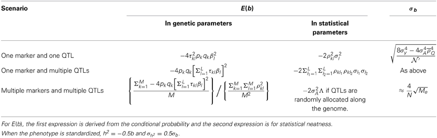
Table 6. Summary of the derivations.

The Additive Variance Component Structure of a Quantitative Trait Without Ascertainment

The additive variance of a trait is defined as ${\sigma }_A^2={\Sigma }_{l=1}^{L}2p_l{q}_l{\beta }_l^2+{\Sigma }_{l_1=1}^L{\Sigma }_{l_2\ne l_1}^{L}2{\rho }_{l_1{l}_2}\sqrt{p_{l_1}{q}_{l_1}{p}_{l_2}{q}_{l_2}}{\beta }_{l_1}{\beta }_{l_2}$. However, for a complex trait with polygenic genetic architecture, if the QTLs are randomly allocated along the genome, ${\sigma }_A^2={\Sigma }_{l=1}^{L}2p_l{q}_l{\beta }_l^2$ (Supplementary Note V), a phenomenon that the between-locus covariances tradeoff. This is often true for a trait without ascertainment or selection. When each QTL is tagged perfectly and randomly allocated along the genome, Λ = 1. Equation (11) zeros out the Δ term and directly gives the unbiased estimate of twice negative of the additive variance. Removing the scale makes the heritability estimate unbiased. In practice, due to imperfect LD, the heritability is reduced to h²Λ.

In fact, the HE regression and the mixed model are equivalent and can agree on the heritability estimate (see Simulation III). However, this equivalence can be disturbed when QTL effects are not randomly distributed (Simulation IV).

Extension to Case-Control GWAS Data

Like the debut application of the original HE regression for schizophrenia (Elston et al., 1973), the IBS HE regression is also extended to case-control GWAS data in this study. However, due to scale issues and ascertainment (Dempster and Lerner, 1950; Falconer, 1966), the estimated heritability needs to be transformed to the liability scale, which is genetically meaningful for ascertained samples. One transformation was proposed by Lee et al. (2011), denoted here as Hong23. It is expressed as $h_l^2=h_o^2\frac{K(1-K)}{z^2}\frac{K(1-K)}{P(1-P)}$, in which h²_l is the heritability on the liability scale, h²_o is the heritability on the observed scale directly estimated based on the case-control data, K is the prevalence of the disease, P is the proportion of the cases in the data, and z is the height of the standard normal distribution in which the prevalence K is located.

Once the heritability is estimated by the HE regression on the observed scale with Hong23, it can be easily transformed from the observed scale to the liability scale. Simulation studies will be conducted to investigate whether the HE regression better estimates heritability than does the mixed linear model (Simulation IV).

In addition, Y in the HE regression can also be expressed as a cross-product, and then E(b) = −2p_kq_kτ²_klβ²_l, which is half that of Equation (7) (See Supplementary Note VI).

Monte Carlo Simulation Results

In the Monte Carlo simulation, we will investigate the precision of the derived equations.

Simulation I: One Marker and One QTL [Evaluation of Equation (7)]

This simulation investigated the accuracy of Equation (7) for a single-marker application. One thousand unrelated individuals were simulated. One marker and one QTL were simulated, both of which were equifrequent and biallelic. The heritability of the QTL was 0.5. The LD between the marker and the QTL was set at three levels: ρ = 0.25, ρ = 0.5, and ρ = 0.75. The single marker was used to construct the genetic relatedness, Ω. Then a single-marker-based HE regression was conducted. After standardizing the phenotype, the negative half of the regression coefficient returned the unbiased heritability estimate.

As indicated by Equation (7), given ρ = 0.25, ρ = 0.5, and ρ = 0.75, the regression coefficient expectation was −0.062, 0.125, and 0.57, respectively. After 100 rounds of simulation, the derived expectation of the regression coefficient, as well as the sampling variance (Table 6), were in good agreement with the simulation results listed in Table 7. This simulation indicates that the single-marker HE regression is a competitive tool for QTL mapping.

TABLE 7

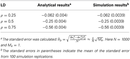
Table 7. Simulation evaluations of Equation (7).

Simulation II: Statistical Power of the Single-Marker HE Regression

For the single-marker HE regression, as the expectation and the sampling variance of the regression coefficient were already derived, a t-test could be constructed as $t=\frac{h^2{\rho }_{kl}^2}{2/N}$, in which the linkage disequilibrium between the k^th marker and the l^th QTL is ρ_kl. When the sample size is sufficiently large, the t-test approaches the z-score distribution, and the non-centrality parameter of χ²₁ is consequently $N\frac{h^2{\rho }_{kl}^2}{4}·N{h}^2{\rho }_{kl}^2~{\chi }_1^2$, a χ²-test with one degree of freedom. In Table 8, the required sample size to detect association with a SNP for a GWAS (type-I error rate of 10⁻⁸) and the required sample size to detect a QTL are indicated.

TABLE 8

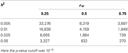
Table 8. The sample size required for the single-marker HE regression to detect a QTL associated with the target marker.

In contrast, for a conventional one-marker association linear regression, y_i = μ + b_ks_ik + e_i, if the phenotype and the genotypes are both standardized, E(b_k) = ρ_klβ_l, and its standard error is ${\sigma }_{b_k}=\sqrt{\frac{{\sigma }_e^2}{N{\sigma }_{s_k}^2}}$, a t-test can be constructed as $t={\rho }_{kl}{\beta }_l/\sqrt{\frac{{\sigma }^2\left(e\right)}{N{\sigma }^2\left(s_k\right)}}=\sqrt{\frac{N{h}^2{\rho }_{kl}^2}{1-h^2{\rho }_{kl}^2}}$. Taking the square of the t statistic, the non-centrality parameter of χ²₁ is $\frac{N{h}^2{\rho }_{kl}^2}{1-h^2{\rho }_{kl}^2}\approx N{h}^2{\rho }_{kl}^2~{\chi }_1^2$.

These two χ² tests differ by the factor $N\frac{h^2{\rho }_{kl}^2}{4}$. Once $N>\frac{4}{h^2{\rho }_{kl}^2}$, the single-marker HE regression is more powerful than the conventional liner regression; otherwise, the conventional linear regression method is more powerful. As listed in Table 9, given that the heritability of a QTL is 0.01, if the LD between the target marker is low (ρ_kl = 0.25), medium (ρ_kl = 0.5), or high (ρ_kl = 0.75), the sample size required to allow HE to outperform the linear regression is 6400, 1600, and 712, respectively. If the heritability is even smaller, say h² = 0.001, the required sample size is 12,800, 3200, and 1423 to make the HE regression more powerful under the low, medium, and high LD, respectively.

TABLE 9

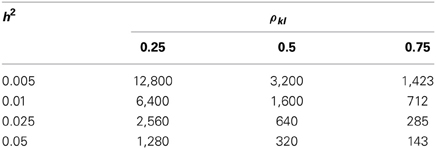
Table 9. The required sample size that makes the HE regression more powerful than the conventional single-marker linear regression.

Depending on the sample size, heritability, and LD patterns between the QTL and the target marker, the power of the HE regression may or may not be greater than the conventional linear regression. However, when the sample size is large, or the heritability of the QTL is large, HE regression is a more powerful tool for association studies. These results are based on the assumption that the real sampling variance agrees with the derived theoretical result.

Simulation III: The All-Marker HE Regression and the Mixed Linear Model are Equivalent [Δ = 0 in Equation (11)]

In this simulation, 100 equifrequent and biallelic QTLs were simulated, and the additive effect of each QTL was sampled from N(0, 1). Four LD levels (ρl₁, l₂ = 0, 0.25, 0.5, 0.75) were adopted for each of two consecutive QTLs, and the effective number of markers decreased correspondingly (M_e ≈ 100, 90, 61, 29). One thousand unrelated individuals were simulated, and the genetic relatedness of each pair of individuals was estimated on these 100 QTLs. The heritability of the simulated polygenic model was 0.5, which is calculated as $h^2=\frac{{\sigma }_A^2}{{\sigma }_A^2+{\sigma }_e^2}$. And ${\sigma }_A^2={\Sigma }_{l=1}^{L}2p_l{q}_l{\beta }_l^2+{\Sigma }_{l_1=1}^L{\Sigma }_{l_2\ne l_1}^{L}2{\rho }_{l_1{l}_2}\sqrt{p_{l_1}{q}_{l_1}{p}_{l_2}{q}_{l_2}}{\beta }_{l_1}{\beta }_{l_2}$.

Both the HE regression and the mixed linear model were employed to estimate the additive variance component. The mixed linear model (Yang et al., 2010) can be expressed as y_i = μ + x_ija_j + e_i, where y_i is the phenotype of the i^th individual, μ is the mean, x_ij is the indicator variable with values of 0, 1, or 2 depending on the reference allele counts, and e_j is the residual. Restricted maximum likelihood (REML) was employed to estimate the variance components of the mixed linear model (Yang et al., 2010).

As shown in Table 10, the estimated heritability from either the HE regression or the mixed linear model was equal and not biased, demonstrating the equivalence between the HE regression and the mixed linear model when the QTLs are randomly distributed regardless of their pairwise LD.

TABLE 10

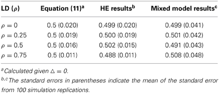
Table 10. Simulation evaluations of Equation (11) and comparison between the HE regression and the mixed linear model method (Δ = 0).

E(b) = −2σ²_A Λ (ignoring Δ) sheds light on the inference of the general LD pattern between the tagged markers and the causal variance. $\Lambda =\frac{{\overline{\rho }}_Q^2}{{\overline{\rho }}_M^2}$, and ρ²_M can be estimated from markers. If the heritability of the trait is known (not likely though), it is possible to estimate ρ²_Q. For example, the heritability of height is estimated at around 0.8 (Visscher et al., 2006; Perola et al., 2007) in linkage, but is 0.4 as estimated in an association study (Yang et al., 2010). If the estimate from linkage was considered to be the true heritability, $\widehat{\Lambda }$ = 0.5. Assuming the effective number of markers is M_e = 10,000, ρ²_M = 0.0001, ρ²_Q = $\widehat{\Lambda }$ρ²_M = 0.00005. The average absolute value of the LD between a QTL and a marker is 0.007.

Simulation IV: When the HE Regression and the Mixed Linear Model are Not Equivalent [when Δ ≠ 0 in Equation (11)]

The general setting for this simulation was similar to the last one, but the QTL effects were sorted such that the additive effects were increased along the simulated chromosomal segment. The covariance between any two QTLs can be predicted by cov. The heritability is defined as $h^2=\frac{{\sigma }_A^2}{{\sigma }_A^2+{\sigma }_e^2}$, in which ${\sigma }_A^2={\Sigma }_{l=1}^{L}2p_l{q}_l{\beta }_l^2+{\Sigma }_{l_1=1}^L{\Sigma }_{l_2\ne l_1}^{L}2{\rho }_{l_1{l}_2}\sqrt{p_{l_1}{q}_{l_1}{p}_{l_2}{q}_{l_2}}{\beta }_{l_1}{\beta }_{l_2}$. Different from the last simulation, $\Delta =-2{\Sigma }_{k=1}^M({\Sigma }_{l_1=1}^L{\Sigma }_{l_2\ne l_1}^{L}2{\rho }_{k{l}_1}{\rho }_{k{l}_2}{\sigma }_{l_1}{\sigma }_{l_2})/M\ne 0$.

With this set-up, which is not likely to be true in practice but illustrates an extreme case, the HE regression and the mixed model gave very different estimations. With increased correlation between markers, the HE gave inflated estimates and the mixed model gave deflated estimates. Although both methods gave biased estimates, Equation (11) still could predict the results of the HE regression correctly (See Table 11).

TABLE 11

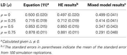
Table 11. Simulation evaluations of Equation (11) when the covariance summation is not zero (Δ ≠ 0).

Simulation V: Application to Case-Control Data

The HE regression was applied to case-control data. A polygenic model of L equifrequent diallelic QTLs was simulated, and each locus was in Hardy–Weinberg equilibrium and any pair of QTLs was in linkage equilibrium. The heritability on the liability scale was h²_l, the heritability on the liability scale. The effect of each QTL was sampled from N(0, σ²_b), and σ²_b = h_l² /[2 × p × (1 − p) × L], in which p = 0.5. The phenotype of each individual under the liability scale was scaled to unit. The ascertainment of cases on the liability scale was K. Individuals were sampled from the described reference population until 1000 cases and 1000 controls were recruited.

The heritability on the liability scale was 0.5. In order to cover a broad range of scenarios, three levels of QTL number, L = 100, 1000, and 10,000, and three levels of disease prevalence at the population level, K = 0.1, 0.01, and 0.001, were adopted. Nine scenarios were simulated in total, and 30 independent simulation replications were implemented for each scenario.

The genetic relationship matrix was constructed using all individuals and the allele frequencies were estimated from the sample. The genetic additive variance components were estimated with the HE regression and the mixed model method. As the directly estimated variance component was on the observed scale and could be greater than 1, we employed both the REML and non-constrained REML for mixed model methods, which allowed the heritability to be greater than 1.

As illustrated in Figure 1, the estimated h²_l was compared across all three methods. In general the HE regression resulted in a more precise estimate than that of the REML and non-constrained REML. For the mixed model methods, either with or without constraints, REML often underestimated the variance components. The bias was caused by two factors: the number of QTLs (in each row panel) and the prevalence of the disease (in each column panel). With fewer QTLs, a lower prevalence could exacerbate underestimation by the mixed model.

FIGURE 1

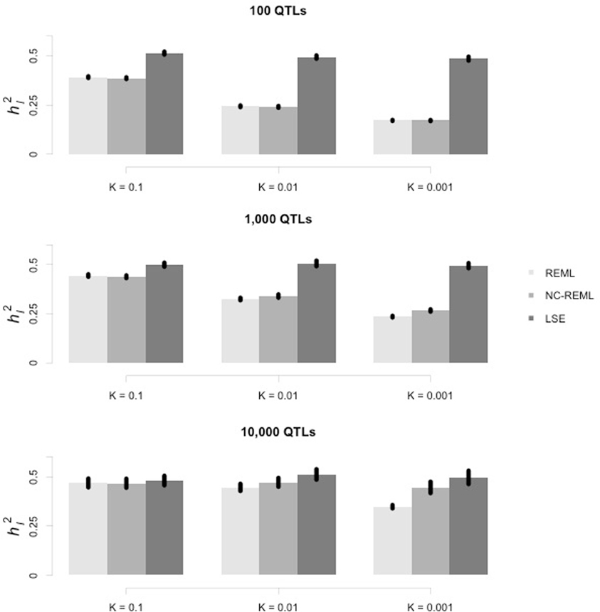
Figure 1. Estimation of heritability on the liability scale using the HE regression and mixed linear model methods. In each row, from left to right, each panel represents the case-control sample simulated under the same heritability on the liability scale (h²_l) but with different prevalence. In each panel, the vertical axis indicates the estimated heritability on the liability scale (h²_l), whereas the horizontal axis indicates which of the three methods (REML, non-constrained REML, and HE regression [least square estimate]) was used. The standard error of the mean (SEM) is indicated at the top of each bar.

Conclusion

The analytical results summarized in Table 6 were evaluated using Monte Carlo simulation, and were highly precise in general. The single-marker HE regression is a competitive tool for QTL mapping, particularly with a large sample size (Simulations I, II). The HE regression and the mixed model method were equivalent, with both providing a precise heritability estimate for a typical polygenic trait (Simulation III). However, if QTL effects are correlated, neither the HE regression nor the mixed model method gave an unbiased estimate (Simulation IV). For case-control studies, the HE regression should be preferred in general (Simulation V).

Genetic Analysis Repository (GEAR)

In order to facilitate application of the HE regression method to estimate complex trait heritability, GEAR software was developed. GEAR was developed on Java and can run across many operating systems, such as Windows, Mac, and Linus/Unix, as long as a Java virtual machine is available. GEAR has been demonstrated to function in the following situations.

(1) It can generate genetic relatedness of unrelated individuals, as formulated in Equation (3), based on whole-genome markers.

(2) It can estimate the effective number of markers based on a genetic-relatedness matrix.

(3) It can estimate heritability with the HE regression. GEAR can read genotype data saved in PLINK binary format (Purcell et al., 2007).

GEAR can be downloaded from the website: https://sourceforge.net/projects/gbchen/files/GEAR/

The online GEAR manual can be found at https://sourceforge.net/p/gbchen/wiki/GEAR/

Discussion

Historically, linkage was the major tool for QTL mapping of complex traits since the 1970s, which was gradually replaced by association analysis when GWAS became popular (The Wellcome Trust Consortium, 2007). The transmission/disequilibrium test (TDT; Ott, 1989; Spielman et al., 1993) triggered the transition from linkage to association for family-based studies. In the year 2000, generalized TDT was proposed (Laird et al., 2000), which is robust for population stratification. Shortly after that, population-based design emerged as the major flow in genetic data, and GWAS became the leading method for estimating heritability up until now. Extension of the original HE regression to association studies can be seen as an effort to increase the diversity of GWAS analysis tools.

In this study, we established a theory for a modified HE regression, in which IBS scores replace IBD scores. Although IBS is used to detect IBD in linkage studies (Lange, 1986a,b; Bishop and Williamson, 1990), it is considered to be a way of inferring IBD for relatives, such as sib pairs, when founder genotypes are unavailable. In this study, IBS served as the key concept to detect association of unrelated samples rather than relatives. Linkage and association have both been proposed to estimate heritability of complex traits. For example, for height, the heritability estimated from linkage studies is around 0.8 (Visscher et al., 2006; Perola et al., 2007), but around 0.4 from association studies (Yang et al., 2010). Thus, far there is no clear conclusion regarding the fundamental difference between the heritability estimated from these two kinds of methods. Despite their mathematical similarity, application, and interpretation differences should be appreciated.

Under various scenarios, the mathematical expectations of the regression coefficients, as well as the sampling variances, were derived. There is substantial mathematical similarity between the IBD HE regression and the IBS HE regression. For example, for both models under the single-marker scenario, their regression coefficients can be expressed in a unified form, E(b) = − 2ρ² σ²_A. As these two models are based on different genetic mechanisms, the interpretations of their respective regression coefficients are reasonably different. In the IBD-based HE regression, E(b) = −2(1 − 2c)² σ_Al², 1 − 2c ranges from 0 to 1; whereas in the IBS-based HE regression, E(b) = −2τ²_kl σ_Al², in which τ_kl, ranges from −1 to 1. As the values of r and R rely upon the allele frequencies of the biallelic marker and the biallelic QTL, they reach either −1 or 1 only given that the marker has the same allele frequency as that of the QTL. However, after taking the square, both (1 − 2c)² and τ² lie between 0 and 1, inclusive.

Equation (11), E(b) = −2σ²_A Λ (ignoring Δ), provides a possible way to estimate the LD pattern between causal loci and markers. If the true heritability is not readily known, it is possible to estimate ρ²_Q, the average LD between QTLs and markers. As demonstrated in simulation III, it may be possible to estimate ρ². However, the causal loci can be in any possible form, such as SNPs, chromatin markers, or methylation markers, and different methods capture genetic variation in different forms. In practice, the obstacle in estimating ρ² lies in how heritability estimated from different methods, such as linkage and association, or genotyping platforms, such as SNP markers and methylation markers, can be connected to each other. Equation (11) sheds light on the investigation for how QTLs are distributed along the genome.

Application of the HE regression to heritability estimation of complex traits revealed that the HE regression seems to be equivalent to the mixed model approaches in general (Δ = 0). A similar equivalence was previously established for linkage analysis (Sham and Purcell, 2001). However, for GWAS data, it should be noted that the equivalence is conditional on the genetic architecture of a trait. As indicated in the simulation, the equivalence stands only for typical polygenic genetic architecture, which may be true for many traits without ascertainment or selection, such as height (Yang et al., 2010). However, when substantial covariance exists between causal loci, the equivalence does not stand and neither the HE regression nor the mixed model method gave unbiased estimates. The equivalence may break down under other circumstances that have not been investigated. In real studies, this kind of covariance may be a result of selection in active regions, such as HLA loci, which harbors many signals; then, the HE regression and the mixed model estimates may differ. The equivalence may break down under other circumstances that have not been investigated in this study.

In GWAS, many samples are collected for complex diseases, which are often in a case-control design. Complex disease prevalence is often low; consequently, the cases are under strong ascertainment, which disrupts the assumptions underlying the mixed linear model. As observed in the simulation studies, the HE regression is more precise in estimating heritability than the mixed linear model for case-control studies across a broad range of scenarios. Use of HE regression is advantageous when the disease prevalence is low and the number of causal loci is few. In their original work, Lee et al. (2011) assumed an infinitesimal model of complex diseases. However, when this assumption was disrupted during simulation (likely in practice as well), the mixed linear model method gave biased estimates of heritability. Thus, whenever possible, the HE regression method is preferable to estimate heritability of complex traits.

As derived in this work, the HE regression and the mixed model method are equivalent under polygenic genetic architecture. In other words, when the estimates generated by these two methods significantly differ for the same data, caveats should be presented. As investigated in the simulation, the real heritability may lie between the estimates of these two methods. Speed et al. (2012) previously investigated the assumptions underlying the mixed model method and proposed alternative weighting methods to adjust the heritability estimation. However, as their weighting method depends on genetic architecture, which is often unknown, it is difficult to justify which weighting method is appropriate to adopt for certain data (Gusev et al., 2013). Thus, simply comparing the estimates from the HE regression and the mixed model method may offer an alternative way of justification.

It should be noted that the HE regression method is on the basis of the least square framework rather than the maximal likelihood framework as many mixed model based on (Yang et al., 2010; Speed et al., 2012; Lee et al., 2013). As a numerical method, maximal likelihood methods give estimates optimizing the likelihood under the assumptions, which may break down in practice. Given recent interests in comparing estimates with or without imputation for the genome (Gusev et al., 2013), controversial results have been observed. It is not sure what the increased or decreased estimation of heritability indicates after imputation. A reasonable guess will be that the local covariance structure, as indicated in Equation (11), changes and eventually bring out different estimates. The proposed IBS HE regression, which depends on fewer assumptions compared with maximal likelihood methods, may help melt the controversy.

In practice, undocumented relatedness may creep into samples, and eventually bring about suspiciously high relatedness. As discussed previously (Powell et al., 2010), Equation (3) gives a score of 0 for a pair of unrelated individuals, 0.5 for first-degree relatives, and 1 for duplicated individuals or monozygotic twins. It seems easy to eliminate related individuals if a cutoff, say a relatedness of less than 0.05, is applied to the sample. For association studies, population stratification may increase false positive rates. To reduce the threat of population stratification, phenotypes can be adjusted by principal components (Price et al., 2006) and then fit into the HE regression. If a sample is admixed, the power of the HE regression may be reduced if, in the ancestral populations, the allele frequency spectrums are different from each other or genetic heterogeneity exists in the genetic architecture of the underlying trait in question. More investigation will be required to overcome this challenge.

The variance components have often been estimated via REML (Yang et al., 2010; Lee et al., 2011). Given its various merits, REML is computationally expensive, particularly for large sample sizes. The computational complex is on the scale of O(tN³), which indicates that it is cubic to the sample size and t rounds of iterations. The time complex of the HE regression is far lower, asymptotically O(2N²), given two parameters, the intercept and the regression coefficient, included in the model. Given the large sample sizes often employed in GWAS, the computational burden can be dramatically reduced. Although the HE regression method is derived on a simple-regression scenario, its extension to a multiple-regression scenario is straightforward. For instance, the genetic relatedness between each pair of individuals can be constructed on each chromosome and then all chromosome-based relatedness scores can be fit into the regression framework. In addition, the difference between a pair of phenotypes can also be expressed as a cross product and squared sum (Sham and Purcell, 2001).

Author Contributions

Guo-Bo Chen conceived the study, derived the equations, conducted the simulation studies, and calculated the analytical results. Guo-Bo Chen developed and maintained the GEnetic Analysis Repository (GEAR) software. Guo-Bo Chen wrote the manuscript.

Conflict of Interest Statement

The author declares that the research was conducted in the absence of any commercial or financial relationships that could be construed as a potential conflict of interest.

Acknowledgments

This article benefited greatly from detailed feedback by reviewers. Thanks to Professors Peter M. Visscher and Naomi R. Wray for helpful discussion. Thanks to Mr. Zhi-Xiang Zhu for contributing to GEAR. The publication fee was in part covered by Frontiers Publishing Grants and by Australia National Health and Medical Research Council Grant 1011506 to Peter M. Visscher and Naomi R. Wray.

Supplementary Material

The Supplementary Material for this article can be found online at: http://www.frontiersin.org/journal/10.3389/fgene.2014.00107/abstract

References

Bishop, D. T., and Williamson, J. A. (1990). The power of identity-by-state methods for linkage analysis. Am. J. Hum. Genet. 46, 254–265.

Pubmed Abstract | Pubmed Full Text

Dempster, E. R., and Lerner, I. M. (1950). Heritability of threshold characters. Genetics 35, 212–236.

Pubmed Abstract | Pubmed Full Text

Devlin, B., and Risch, N. (1995). A comparison of linkage disequilibrium measures for fine-scale mapping. Genomics 29, 311–322. doi: 10.1006/geno.1995.9003

Pubmed Abstract | Pubmed Full Text | CrossRef Full Text

Elston, R. C., Kringlen, E., and Namboodiri, K. K. (1973). Possible linkage relationships between certain blood groups and schizophrenia or other psychoses. Behav. Genet. 3, 101–106. doi: 10.1007/BF01067650

Pubmed Abstract | Pubmed Full Text | CrossRef Full Text

Falconer, D. S. (1966). The inheritance of liability t o certain diseases, estimated from the incidence among relatives. Ann. Hum. Genet. 29, 51–76.

Gusev, A., Bhatia, G., Zaitlen, N., Vilhjalmsson, B. J., Diogo, D., Stahl, E. A., et al. (2013). Quantifying missing heritability at known GWAS loci. PLoS Genet. 9:e1003993. doi: 10.1371/journal.pgen.1003993

Pubmed Abstract | Pubmed Full Text | CrossRef Full Text

Haseman, J. K., and Elston, R. C. (1972). The investigation of linkage between a quantitative trait and a marker locus. Behav. Genet. 2, 3–19. doi: 10.1007/BF01066731

Pubmed Abstract | Pubmed Full Text | CrossRef Full Text

Hill, W. G., and Robertson, A. (1968). Linkage disequilibrium in finite populations. Theor. Appl. Genet. 38, 226–231. doi: 10.1007/BF01245622

Pubmed Abstract | Pubmed Full Text | CrossRef Full Text

Hill, W. G., and Weir, B. S. (2011). Variation in actual relationship as a consequence of Mendelian sampling and linkage. Genet. Res. (Camb.). 93, 47–64. doi: 10.1017/S0016672310000480

Pubmed Abstract | Pubmed Full Text | CrossRef Full Text

Laird, N. M., Horvath, S., and Xu, X. (2000). Implementing a Unified Approach Tests of Association to family-based tests of association. Genet. Epidemiol. 19, S36–S42. doi: 10.1002/1098-2272(2000)19:1+<::AID-GEPI6>3.0.CO;2-M

Pubmed Abstract | Pubmed Full Text | CrossRef Full Text

Lange, K. (1986a). A test statistic for the affected-sib-set method. Ann. Hum. Genet. 50, 283–90. doi: 10.1111/j.1469-1809.1986.tb01049.x

Pubmed Abstract | Pubmed Full Text | CrossRef Full Text

Lange, K. (1986b). The affected sib-pair method using identity by state relations. Am. J. Hum. Genet. 39, 148–150.

Pubmed Abstract | Pubmed Full Text

Lee, S. H., Wray, N. R., Goddard, M. E., and Visscher, P. M. (2011). Estimating missing heritability for disease from genome-wide association studies. Am. J. Hum. Genet. 88, 294–305. doi: 10.1016/j.ajhg.2011.02.002

Pubmed Abstract | Pubmed Full Text | CrossRef Full Text

Lee, S. H., Yang, J., Chen, G.-B., Ripke, S., Stahl, E. A., Hultman, C. M., et al. (2013). Estimation of SNP heritability from dense genotype data. Am. J. Hum. Genet. 93, 1151–1155. doi: 10.1016/j.ajhg.2013.10.015

Pubmed Abstract | Pubmed Full Text | CrossRef Full Text

Lynch, M., and Walsh, B. (1998). Genetics and Analysis of Quantitative Traits. Sunderland, MA: Sinauer Associates, Inc.

Manolio, T. A., Collins, F. S., Cox, N. J., Goldstein, D. B., Hindorff, L. A., Hunter, D. J., et al. (2009). Finding the missing heritability of complex diseases. Nature 461, 747–753. doi: 10.1038/nature08494

Pubmed Abstract | Pubmed Full Text | CrossRef Full Text

Ott, J. (1989). Statistical properties of the haplotype relative risk. Genet. Epidemiol. 6, 127–130. doi: 10.1002/gepi.1370060124

Pubmed Abstract | Pubmed Full Text | CrossRef Full Text

Perola, M., Sammalisto, S., Hiekkalinna, T., Martin, N. G., Visscher, P. M., Montgomery, G. W., et al. (2007). Combined genome scans for body stature in 6,602 European twins: evidence for common Caucasian loci. PLoS Genet. 3:e97. doi: 10.1371/journal.pgen.0030097

Pubmed Abstract | Pubmed Full Text | CrossRef Full Text

Powell, J. E., Visscher, P. M., and Goddard, M. E. (2010). Reconciling the analysis of IBD and IBS in complex trait studies. Nat. Rev. Genet. 11, 800–805. doi: 10.1038/nrg2865

Pubmed Abstract | Pubmed Full Text | CrossRef Full Text

Price, A. L., Patterson, N. J., Plenge, R. M., Weinblatt, M. E., Shadick, N. A., and Reich, D. (2006). Principal components analysis corrects for stratification in genome-wide association studies. Nat. Genet. 38, 904–909. doi: 10.1038/ng1847

Pubmed Abstract | Pubmed Full Text | CrossRef Full Text

Purcell, S., Neale, B., Todd-Brown, K., Thomas, L., Ferreira, M. A. R., Bender, D., et al. (2007). PLINK: a tool set for whole-genome association and population-based linkage analyses. Am. J. Hum. Genet. 81, 559–575. doi: 10.1086/519795

Pubmed Abstract | Pubmed Full Text | CrossRef Full Text

Purcell, S. M., Wray, N. R., Stone, J. L., Visscher, P. M., O'Donovan, M. C., Sullivan, P. F., et al. (2009). Common polygenic variation contributes to risk of schizophrenia and bipolar disorder. Nature 460, 748–752. doi: 10.1038/nature08185

Pubmed Abstract | Pubmed Full Text | CrossRef Full Text

Ritland, K. (1996). Estimators for pairwise relatedness and individual inbreeding coefficients. Genet. Res. 67, 175–185. doi: 10.1017/S0016672300033620

Pubmed Abstract | Pubmed Full Text | CrossRef Full Text

Sham, P. C., and Purcell, S. (2001). Equivalence between Haseman-Elston and variance-components linkage analyses for sib pairs. Am. J. Hum. Genet. 68, 1527–1532. doi: 10.1086/320593

Pubmed Abstract | Pubmed Full Text | CrossRef Full Text

Sham, P. C., Purcell, S., Cherny, S. S., and Abecasis, G. R. (2002). Powerful regression-based quantitative-trait linkage analysis of general pedigrees. Am. J. Hum. Genet. 71, 238–253. doi: 10.1086/341560

Pubmed Abstract | Pubmed Full Text | CrossRef Full Text

Speed, D., Hemani, G., Johnson, M. R., and Balding, D. J. (2012). Improved heritability estimation from genome-wide SNPs. Am. J. Hum. Genet. 91, 1011–1021. doi: 10.1016/j.ajhg.2012.10.010

Pubmed Abstract | Pubmed Full Text | CrossRef Full Text

Spielman, R. S., McGinnis, R. E., and Ewens, W. J. (1993). Transmission test for linkage disequilibrium: the insulin gene region and insulin-dependent diabetes mellitus (IDDM). Am. J. Hum. Genet. 52, 506–516.

Pubmed Abstract | Pubmed Full Text

The Wellcome Trust Consortium. (2007). Genome-wide association study of 14,000 cases of seven common diseases and 3,000 shared controls. Nature 447, 661–678. doi: 10.1038/nature05911

Pubmed Abstract | Pubmed Full Text | CrossRef Full Text

Vinkhuyzen, A. A. E., Wray, N. R., Yang, J., Goddard, M. E., and Visscher, P. M. (2013). Estimation and partition of heritability in human populations using whole-genome analysis methods. Annu. Rev. Genet. 47, 75–95. doi: 10.1146/annurev-genet-111212-133258

Pubmed Abstract | Pubmed Full Text | CrossRef Full Text

Visscher, P. M., Medland, S. E., Ferreira, M. A. R., Morley, K. I., Zhu, G., Cornes, B. K., et al. (2006). Assumption-free estimation of heritability from genome-wide identity-by-descent sharing between full siblings. PLoS Genet. 2:e41. doi: 10.1371/journal.pgen.0020041

Pubmed Abstract | Pubmed Full Text | CrossRef Full Text

Weeks, D. E., and Lange, K. (1988). The affected-pedigree-member method of linkage analysis. Am. J. Hum. Genet. 42, 315–326.

Pubmed Abstract | Pubmed Full Text

Wray, N. R. (2005). Allele frequencies and the r2 measure of linkage disequilibrium: impact on design and interpretation of association studies. Twin Res. Hum. Genet. 8, 87–94. doi: 10.1375/1832427053738827

Pubmed Abstract | Pubmed Full Text | CrossRef Full Text

Yang, J., Benyamin, B., McEvoy, B. P., Gordon, S., Henders, A. K., Nyholt, D. R., et al. (2010). Common SNPs explain a large proportion of the heritability for human height. Nat. Genet. 42, 565–569. doi: 10.1038/ng.608

Pubmed Abstract | Pubmed Full Text | CrossRef Full Text

Yang, J., Weedon, M. N., Purcell, S., Lettre, G., Estrada, K., Willer, C. J., et al. (2011). Genomic inflation factors under polygenic inheritance. Eur. J. Hum. Genet. 19, 807–812. doi: 10.1038/ejhg.2011.39

Pubmed Abstract | Pubmed Full Text | CrossRef Full Text