Path Choice Models in Stochastic Assignment: Implementation and Comparative Analysis

In assignment models, a key role is played by the path choice simulation that evaluates the path chosen by users in relation to the perceived paths and relative costs. This study deals with the effects of the implementation of some most adopted path choice models (Logit, Weibit, Probit, and Gammit) within a Stochastic User Equilibrium assignment procedure. Some considerations on parameters needed to make results comparable and the method used to estimate them are also suggested some extensions based on Weibit model are proposed. Results obtained both on a test network and on a real one are reported.

1 Introduction

In this study, the simulation of the users’ path choice behavior is evaluated by considering different random utility models (RUM).

Path choice is simulated once the origin and destination of the travel, the departure time, and the transport mode have been defined. It is a component of assignment models that can be formulated as a combination of a demand model and a supply model that, in the search for equilibrium between demand and supply, leads to a fixed-point problem (Cantarella, 1997). It is generally assumed that users perceive trip time or cost in a random form. Different authors have considered the statistical distributions of the perceived trip times as belonging to different families.

Starting from the generalized extreme value (GEV) class of models, proposed by McFadden (1978), many models for path choice have been formulated, such as multinomial Logit, C-Logit, path-size Logit, nested Logit, cross-nested Logit, and link-nested models (Manski and McFadden, 1981; Ben-Akiva and Lerman, 1985; Cascetta et al., 1996; Ben-Akiva and Bierlaire, 1999), where Gumbel-distributed random costs are considered. The main advantage of assuming the GEV distributions is that these models are closed under maximization, which means a simple and tractable choice function. Castillo et al. (2008) introduced a closed-form expression for the choice probabilities in the case of independent Weibull-distributed random costs.

By introducing a more general structure of the covariance matrix of the joint distribution of the random residuals (and of the utilities), Daganzo and Sheffi (1977), Sheffi (1985), Rosa and Maher (2002), Yai et al. (1997), and Sheffi and Powell (1982) analyzed the probit model that assumes a normal distribution. Cantarella and Binetti (2002) analyzed the gammit model that assumes a gamma distribution in order to avoid positive perceived utility values, as allowed by a normal distribution. Recently, considering the lack of information on one or more alternatives, other classes of path choice models have been proposed, such as quantum utility models (QUM) (Vitetta, 2016; Di Gangi and Vitetta, 2018) and fuzzy utility models (De Maio and Vitetta, 2015).

Aim of this study is to analyze the effects of the practical implementation of different path choice models based on random utility theory (Logit, Weibit, Probit, and Gammit) within a stochastic user equilibrium (SUE) assignment procedure. Particular attention was paid to the parameters needed to make results from different models comparable. The path choice models are crucial for the assignment models, both for private vehicles (Cantarella and Fiori, 2022; Wang et al., 2019; Di Gangi et al., forthcoming) and transit (Nuzzolo and Comi, 2016; Nuzzolo and Comi, 2018). There are two main approaches: explicit path enumeration or implicit path enumeration (Quattrone and Vitetta, 2011). In implicit field can be cited (Russo and Vitetta, 2003; Antonisse et al., 1989) while in explicit field can be cited (Fosgerau et al., 2013; Mai et al., 2015; Comi and Polimeni, 2022). A review on path choice models is reported in (Prashker and Bekhor, 2004) and (Prato, 2009).

The main original contributions of this study are as follows:

• extensions of a stochastic loading procedure based on path costs following a Weibull distribution with the implementation of a weibit loading procedure that does not require explicit path enumeration;

• some considerations on how to define model parameters in order to make results comparable;

• a comparison of the performances of the considered models obtained both on a test and on a real network.

The advantage in using a Weibull distribution is twofold: 1) the choice probability can be calculated in a closed form, and 2) the dependence of the variance on the path cost allows having different variance values for different o/d pairs, overcoming the issue of Logit models where the variance is the same for all o/d pairs.

Considering the structure of this article, in Section 2, after the description of some requirements for path choice models (2.1), a short summary of the considered RUM (2.2) and some operational considerations regarding the implementation of the considered path choice models (2.3) are described. In Section 3, which concerns stochastic network assignment, an extension based on the weibit model is reported, particularly a loading procedure that does not require explicit path enumeration. In Section 4, some results obtained by carrying out tests both on a simple network (4.1) and on a real network (4.2) are presented. In this last case, results are compared by considering the performances obtained on a real system. Finally, Section 5 contains a summary of the obtained results and some indications for further developments.

2 Modeling Path Choice Behavior

2.1 Requirements for Path Choice Models

Following (Cantarella et al., 2020), some requirements useful in classifying path choice models are, for the convenience of the reader, summarized in the following, where the classification of the requirements is carried out both from a mathematical and modeling point of view. It is worth noting that these requirements hold whatever is the theory behind the path choice models. In this paper, path choice models derived from the theory of random utilities will be considered.

2.1.1 Mathematical Requirements

Under the assumptions of linear utility functions, mathematical requirements allow effectively modeling any choice behavior. Considering, in particular, a path choice model, the main requirements are the continuity and monotonicity of the utility function. Then, the model can be specified by a function if the values and random residuals of the perceived utility are assumed distributed as continuous random variables with a nonsingular covariance matrix. In order to guarantee that small changes of path costs induce small changes of choice probabilities, the continuity of the path choice model must be assured (note that if the model is also differentiable, the Jacobian is continuous). This feature, assured by commonly used joint probability density functions, guarantees the continuity of the resulting arc flow function. Thus, it is useful to state the existence of SUE. The assurance that an increase in cost of a path corresponds to a decrease of its choice is given by the monotonicity of the path choice function. More generally, the path choice function should be nonincreasing monotone with respect to path costs. This feature guarantees the monotonicity of the resulting arc flow function. Thus, it is useful to state the uniqueness of the solution of SUE. If any change of the scale of the utility does not affect the model, the choice model has the independence from linear transformations of utility property.

2.1.2 Modeling Requirements

Modeling requirements are also useful to effectively simulate path choice behavior. Considering the similarity of perception of partially overlapping paths allows us to avoid counter-intuitive results. In the case of two partially overlapping paths, a positive covariance between them can simulate their similarity because they are likely not perceived as two totally separated paths. This covariance can be specific to the distribution (e.g., Probit and Gammit) or can be induced through modifications of utilities (e.g., C-Logit, path-size Logit, and C-Weibit; the latter is introduced later in this article).

Considering the network model, if an arc can be divided into subarcs, redefining arc costs so that path costs are not affected, this does not affect the perceived utility or random residual distribution of paths and, consequently, choice probabilities. Because this requirement makes reference to the features of the distribution of the sum of random variables, two approaches can be identified to specify perceived utility distribution: 1) direct formulations of probabilistic path choice models, where the distribution of path-perceived utility or random residuals is explicitly specified, and 2) indirect formulations, where path-perceived utility or random residual distribution is specified as a linear combination of arc-perceived utilities (specifying their distribution), even though the analysis of path choice behavior is still carried out at the path level. The independence from arc segmentation mainly requires the use of reproductive random variables. For instance, the sum of several independently distributed normal random variables is still a normal random variable, with the mean given by the sum of the means and variance by the sum of the variances. This feature is also shown by independently distributed gamma random variables with the same variance-to-mean ratio. In both cases, if the arcs in a path are further segmented, provided that the mean path cost and the variance are not affected by segmentation, the resulting path-perceived utility distribution (and then the choice probability) is not affected by segmentation. Generally, the arc flow function with any arc-formulated choice model can be easily computed, if arc-perceived utilities are assumed independently distributed, through Monte Carlo techniques (introduced by Burrel, 1968; see also Sheffi, 1985). Traveling along a path, users perceive a cost that is usually considered a negative utility. The negativity of perceived utility assures that no user perceives a positive utility to travel along any path. This feature can be assured by assuming lower bounded random distributions (for instance log-normal or gamma). If this feature is not presented, it means that a nonelementary path may be a better choice than the elementary path within it, possibly leading to unrealistic situations (a part from some algorithmic drawbacks).

2.1.3 Notations

For the convenience of the reader, Table 1 reports the symbols (grouped by type) used throughout the article (in any case, the meaning of each symbol is recalled each time it is used).

TABLE 1

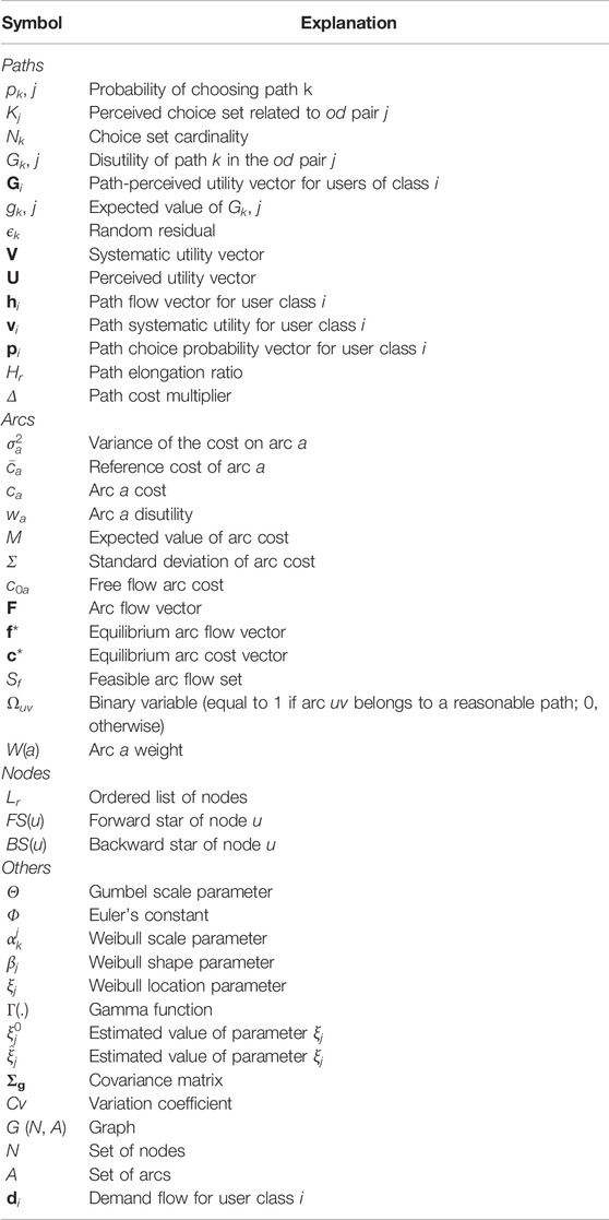
TABLE 1. Symbols.

2.2 Random Utility Path Choice Models

Given an origin/destination (o/d) pair j, the analyst evaluates the probability p_k,j of choosing path k belonging to the perceived choice set of paths K_j. Disutility G_k,j can be expressed as follows:

$G_{k,j}=g_{k,j}+{ϵ}_k(1)$

where g_k,j = E [G_k,j] is the expected value of the disutility (cost) of path k and ϵ_k is the random residual.

Possible models for the evaluation of probabilities (deriving from the hypotheses on random variable G_k,j distribution) are described in the following. Even if they can be classified on the basis of the requirements described in Section 2.1, for the sake of simplicity, description is here conducted on the basis of the existence (or not) of a closed form to define choice probabilities.

2.2.1 Closed-Form Probability Formulation

Multinomial Logit and Weibit model assumptions entail that the covariance matrix of the joint distribution of the random residuals (and of the utilities) is a diagonal matrix with nonzero entries. From a mathematical point of view, Multinomial Logit and Weibit models satisfy the continuity and monotonicity requirements, but independence from linear transformations of utility requirements are not satisfied. From a modelistic point of view, the requirements regarding the similarity of perception of partially overlapping paths are not satisfied because of the general structure of the covariance matrix. In addition, independence from arc segmentation is not assured, and perceived utility distribution is specified in path. The negativity of perceived utility requirement is formally satisfied by multinomial weibit but not by multinomial logit because random residuals, following a Gumbel distribution, can assume negative values (that is a positive disutility), which implies a decrease in path cost.

2.2.1.1 Multinomial Logit

In the Multinomial Logit model, it is assumed that the path costs G_k,j are identical and independently distributed as a Gumbel random variable.

In particular, utility can be expressed as G_k,j = −(g_k,j + ϵ_k), where − g_k,j = E [G_k,j] is the expected value of the utility (cost) of path k, and random residuals -ϵ_k are independently and identically distributed (i.i.d.) as a Gumbel random variable of zero mean and scale parameter θ (Ben-Akiva and Lerman, 1985; Domencich and McFadden, 1975).

The marginal probability distribution function of each random residual can be written as follows Cascetta (2009):

$F_{{ϵ}_k}\left(x\right)=\mathit{exp}\left[-\mathit{exp}\left(-\theta x-\mathrm{\Phi }\right)\right](2)$

where Φ is the Euler’s constant. For multinomial logit, it is assumed that the mean and variance of the Gumbel distribution are, respectively, as follows:

$E\left[{ϵ}_k\right]=0;\mathit{Var}\left[{ϵ}_k\right]=\frac{{\pi }^2}{6\cdot {\theta }^2}\forall j(3)$

The specification of probability for Multinomial Logit is as follows:

$p_{k,j}=\frac{\mathit{exp}\left(-{\theta }_j\cdot g_{k,j}\right)}{{\mathrm{\Sigma }}_{h\in K_j}\mathit{exp}\left(-{\theta }_j\cdot g_{h,j}\right)}(4)$

where θ_j is the distribution parameter related to the choice set K_j.

2.2.1.2 Multinomial Weibit

The Weibit model assumes that the path costs G_k,j are independently distributed as a $Weibull({\xi }_j,{\alpha }_k^j,{\beta }_j)$ random variable, and its probability density function is as follows:

$f\left(x\right)=\frac{{\beta }_j}{{\alpha }_k^j}{\left(\frac{x-{\xi }_j}{{\alpha }_k^j}\right)}^{\left({\beta }_j-1\right)}\cdot \mathit{exp}\left[-{\left(\frac{x-{\xi }_j}{{\alpha }_k^j}\right)}^{\left({\beta }_j\right)}\right](5)$

where

• ${\alpha }_k^j$ is a scale parameter;

• β_j is a shape parameter;

• ξ_j is a location parameter.

The mean and variance are, respectively, as follows:

$E\left[G_{k,j}\right]={\xi }_j+{\alpha }_k^j\cdot \mathrm{\Gamma }\left(1+\frac{1}{{\beta }_j}\right)=g_{k,j}(6)$

$\mathit{Var}\left[G_{k,j}\right]={\left({\alpha }_k^j\right)}^2\left[\mathrm{\Gamma }\left(1+\frac{2}{{\beta }_j}\right)-{\mathrm{\Gamma }}^2\left(1+\frac{1}{{\beta }_j}\right)\right](7)$

where Γ(.) is the gamma function.

The specification of probability for Multinomial Weibit is (Castillo et al., 2008) as follows:

$p_{k,j}=\frac{{\left(g_{k,j}-{\xi }_j^0\right)}^{-{\beta }_j}}{{\mathrm{\Sigma }}_{h\in K_j}{\left(g_{h,j}-{\xi }_j^0\right)}^{-{\beta }_j}}{g}_{k,j}\ge {\xi }_j^0\forall k\in K_j(8)$

where ${\xi }_j^0$ is an estimated value of parameter ξ_j.

2.2.2 Not Closed-Form Probability Formulation

From a mathematical point of view, Probit and Gammit models satisfy the continuity, monotonicity, and independence from linear transformations of utility requirements. From a modelistic point of view, the requirements regarding the similarity of perception of partially overlapping paths are satisfied because they allow for the general structure of the covariance matrix. In addition, independence from arc segmentation is assured, and perceived utility distribution is specified in arc. Because a closed form is not available for the choice behavior model, an unbiased estimate of arc flows can be computed through a Monte Carlo technique by successively averaging several loading to the shortest paths (Sheffi, 1985; Burrel, 1968). The Monte Carlo technique is used as a numerical tool to compute the path choice probabilities or to enhance the corresponding arc flows. To apply this approach, by virtue of independence from arc segmentation, the path-perceived utility distribution is derived from independently distributed arc random costs. For practical purposes, to apply the Probit or the Gammit model, path-perceived utilities G_i can be specified through arc utilities g, whose expected values are the opposite of arc costs, E [g] = −c, say: ${\mathbf{G}}_i={\mathbf{B}}_i^T\mathbf{g}$, where B_i is the arc-path incidence matrix for user class i. If the arc-perceived utilities are independently Normal or Gamma distributed with diagonal covariance matrix Σ_g, the resulting path-perceived utilities are still Normal or Gamma distributed with covariance matrix $\mathbf{\Sigma }={\mathbf{B}}_i^T{\mathbf{\Sigma }}_{\mathbf{g}}{\mathbf{B}}_i$ with nonnull covariance for each pair of partially overlapping paths. Negativity of perceived utility is assured only for gammit because, for probit, random residuals, following a normal distribution, can assume negative values (that is a positive disutility), which implies a decrease in path cost.

2.2.2.1 Probit

The Probit model or multinomial probit model (MNP) results when the random residuals in Eq. 1 are assumed to be multivariate normally distributed with zero mean and arbitrary covariance matrix (Daganzo, 1983). The utility vector U (index of o/d pair is omitted to simplify notation) of dimension N_k is therefore MVN(V, Σ), and its probability density function is therefore the following:

$f\left(\mathbf{V},\mathbf{\Sigma }\right)={\left[{\left(2\pi \right)}^{N_k}\cdot \left|\mathbf{\Sigma }\right|\right]}^{-\frac{1}{2}}\mathit{exp}\left[-\frac{1}{2}{\left(\mathbf{U}-\mathbf{V}\right)}^T{\mathbf{\Sigma }}^{-1}\left(\mathbf{U}-\mathbf{V}\right)\right](9)$

where V is the systematic utility vector.

With the MNP model, the choice probability of path k belonging to the perceived choice set of paths K_j of cardinality N_k is expressed by the following:

$\begin{array}{ll}\hfill p_{k,j}& ={\int }_{U_1<U_k}\dots {\int }_{U_k=-\infty }^{\infty }\dots \hfill \\ \hfill & \dots {\int }_{U_{N_k}<U_k}\frac{exp\left[-\frac{1}{2}{\left(\mathbf{U}-\mathbf{V}\right)}^T{\mathbf{\Sigma }}^{-1}\left(\mathbf{U}-\mathbf{V}\right)\right]}{{\left[{\left(2\pi \right)}^{N_k}\cdot \left|\mathbf{\Sigma }\right|\right]}^{\mathrm{1/2}}}d{U}_1\dots d{U}_{N_k}\hfill \end{array}(10)$

2.2.2.2 Gammit

The Gammit model is obtained by assuming that perceived disutilities are jointly distributed as a nonnegative “shifted” multivariate gamma, with the mean equal to the path costs g_k,j and path covariance matrix Σ. Path formulations of the gammit model may be undetermined because the covariance matrix alone does not completely define the joint probability density function of a multivariate gamma random variable. The adopted formulation was proposed by Cantarella and Binetti (2002). It is an arc formulation that overcomes this drawback and, at the same time, assures independence of arc segmentation and rule out positive perceived utilities for any paths. As in Cantarella and Binetti (2002), let ${\bar{c}}_a$ be the (strictly positive) reference cost on arc a. It is assumed that $0<{\bar{c}}_a\le c_a$, with c_a being the arc cost. The perceived disutility of arc a (−w_a) is assumed distributed as a non-negative shifted gamma variable with the mean given by the arc cost, c_a, variance by ${\sigma }_a^2=\theta {\bar{c}}_a$, proportional to reference arc costs ${\bar{c}}_a>0$, and shifting factor obtained as the difference between the arc cost and reference cost, $(c_a-{\bar{c}}_a)$:

$-w_a\sim \left(c_a-{\bar{c}}_a\right)+Gamma\left({\alpha }_a=\frac{{\bar{c}}_a}{\theta },\beta =\theta \right)(11)$

where α_a and β are, respectively, the shape parameter and the rate parameter of the gamma function.

This means that the arc-perceived disutility is the sum of a nonnegative deterministic term that can depend on arc flows and a nonnegative stochastic term independent from arc flows. The assumption on arc reference costs yields that the corresponding reference cost ${\bar{g}}_k$ on path k is strictly positive and not greater than the path cost, $0<{\bar{g}}_k\le g_k$. Finally, the perceived disutility on path k is marginally distributed as a nonnegative shifted gamma variable:

$-u_{k,j}\sim \left(g_{k,j}-{\bar{g}}_{k,j}\right)+Gamma\left({\alpha }_{k,j}=\frac{{\bar{g}}_{k,j}}{\theta },\beta =\theta \right)(12)$

2.3 Implementation of Path Choice Models

This section focuses on some operational considerations regarding the implementation of the considered path choice models. At the end, an application to a simple test network is conducted in order to compare the performances of the considered models. The parameters used to perform the application depend on the considered model. Then, in this section, the parameters needed to implement each model are identified.

2.3.1 Logit

Logit models are based on the Gumbel distribution and, considering Section 2.2.1.1, are characterized only by the parameter θ, which is estimated starting from the variance of path costs G_k as in Eq. 3. In particular, if Sdev [G_k] is the standard deviation of path cost, a variation coefficient Cv can be introduced as follows:

$Cv=\frac{Sdev\left[G_k\right]}{E\left[G_k\right]}(13)$

It is possible to define the parameter of the Gumbel distribution from Eq. 3 as follows:

$\mathit{Var}\left[G_k\right]={\left(Cv\cdot E\left[G_k\right]\right)}^2\Rightarrow \theta =\frac{\pi }{\sqrt{6}\cdot Cv\cdot E\left[G_k\right]}(14)$

Thus, for the implementation of a logit model, the independent variable to be assumed is Cv.

2.3.2 Weibit

Weibit models are based on a Weibull distribution characterized by three parameters ${\xi }_j,{\alpha }_k^j,{\beta }_j$ (see Section 2.2.1.2).

An estimate of the parameter ξ_j $({\widehat{\xi }}_j)$, suggested in Castillo et al. (2008), is the minimum possible travel time ${\xi }_j^0$ associated with the o/d pair j, that is, ${\widehat{\xi }}_j={\xi }_j^0$.

Starting from Eq. 6, parameter ${\alpha }_k^j$ can be written as follows:

${\alpha }_k^j=\frac{g_{k,j}-{\widehat{\xi }}_j}{\mathrm{\Gamma }\left(1+\frac{1}{{\beta }_j}\right)}(15)$

and replacing Eq. 15 in Eq. 7 yields the following:

$\mathit{Var}\left[G_k\right]={\left(\frac{g_{k,j}-{\widehat{\xi }}_j}{\mathrm{\Gamma }\left(1+\frac{1}{{\beta }_j}\right)}\right)}^2\left[\mathrm{\Gamma }\left(1+\frac{2}{{\beta }_j}\right)-{\mathrm{\Gamma }}^2\left(1+\frac{1}{{\beta }_j}\right)\right](16)$

Once the value of variance is assumed, the value of β_j can be calculated from Eq. 16. Once β_j is known, replacing its value in Eq. 15, it is possible to compute the value of ${\alpha }_k^j$. One example of the procedure for the estimation of the value of β_j is shown in Algorithm 1, where the secant method, which does not require the calculation of derivatives, is used.

Referring to Algorithm 1, the initialization involves to set: 1) the variables b₀ and b₁, 2) the threshold value ι to stop the algorithm, and 3) the initial value of objective function F_n. The procedure is iterated while the objective function F_n is less than ι. At each iteration, a value of β_j is obtained, is calculated the variance corresponding to such a value and when the difference with assumed variance is less than ι the procedure is stopped.

Algorithm 1. Procedure for the estimation of the Weibull distribution parameters.

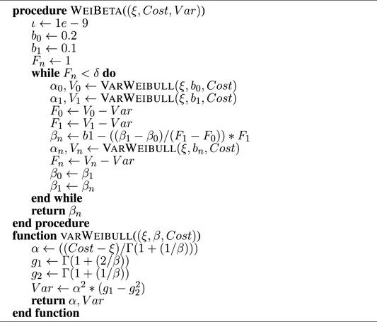
For a practical purpose, owing to a numerical problem that can occur if the difference $(g_{k,j}-{\xi }_j^0)$ is equal to zero, that is, k is the minimum path, a fraction of the minimum cost is considered by means of a multiplier δ < 1, so that:

${\widehat{\xi }}_j=\mathit{min}\left(g_{i,j}\right)\cdot \delta \forall i\in o{d}_j(17)$

Because weibit variance depends, by means of parameter ${\alpha }_k^j$, on the value of path cost, in order to estimate a value of β_j common for all paths making up the choice set of o/d pair j, the arithmetic average of the costs of the paths belonging to the choice set has been considered an estimate of expected value E [G_k], so that:

$\mathit{Var}\left[G_k\right]={\left(Cv\cdot \frac{1}{|K_j|}\sum _{k\in K_j}{g}_{k,j}\right)}^2(18)$

where K_j is the choice set related to the o-d pair j.Thus, for the implementation of a weibit model, the independent variables to be assumed are Cv and δ.

2.3.3 Probit

As discussed in 2.2.2, the path-perceived utility distribution is derived from independently distributed arc random costs that, for the Probit model, follow a normal distribution characterized by the two parameters μ and σ. For a specific case, the expected value and standard deviation can be expressed as follows:

$\mu =c_a;\sigma =Cv\cdot c_{0a}(19)$

where

c_a is the arc cost;

c_0a is the free flow arc cost;

Cv is the variation coefficient.

As discussed above, the Monte Carlo technique is implemented by successive averaging several loading to the shortest paths, so a Nit number of samples have to be carried out. Thus, for the implementation of a probit model, the independent variables to be assumed are Cv and Nit.

2.3.4 Gammit

As discussed in 2.2.2, the path-perceived utility distribution is derived from independently distributed arc random costs that, for the Gammit model, follow a gamma distribution. Following the formulation adopted in 2.2.2.2, a gamma distribution is based on two parameters, which are the following: α > 0 (shape parameter) and β > 0 (rate parameter), and the expected value and variance can be expressed as follows:

$E\left[X\right]=\alpha /\beta ;\mathit{Var}\left[X\right]=\alpha /{\beta }^2(20)$

For a specific case, the expected value and variance can be expressed as follows:

$E\left[X\right]=c_a;\mathit{Var}\left[X\right]={\left(Cv\cdot c_{0a}\right)}^2(21)$

where

c_a is the arc cost;

c_0a is the free flow arc cost;

Cv is the variation coefficient.

Thus, the distribution parameters can be estimated as follows:

$\alpha =\frac{{\left(c_a\right)}^2}{{\left(Cv\cdot c_{0a}\right)}^2};\beta =\frac{c_a}{{\left(Cv\cdot c_{0a}\right)}^2}(22)$

In addition, in this case, the Monte Carlo technique is implemented by successive averaging several loading to the shortest paths, so a Nit number of samples have to be carried out. Thus, for the implementation of a gammit model, the independent variables to be assumed are Cv and Nit.

3 Stochastic Network Assignment

Transportation supply models express how user behavior affects network performances. They are usually based on congested network models, that is, a graph G (N, A) with a transportation cost c_a and a flow f_a associated to each arc a in set A. Let B_i be the arc-path incidence matrix for user class i with entries b_ak = 1 if arc a belongs to path k, b_ak = 0 otherwise; d_i ≥ 0 be the demand flow for user class i; h_i ≥ 0 be the path flow vector for user class i, with entries h_k, k ∈ K_i; f ≥ 0 be the arc flow vector, with entries f_a, a ∈ A; c be the arc cost vector, assumed below with nonnegative entries c_a, a ∈ A; g_i ≥ 0 be the path cost vector for user class i, with entries w_k, k ∈ K_i; the following three equations completely describe the transportation supply:

$\mathbf{f}={\mathrm{\Sigma }}_i{\mathbf{B}}_i{\mathbf{h}}_i(23)$

$\mathbf{c}=\mathbf{c}\left(\mathbf{f}\right)(24)$

${\mathbf{g}}_i={\mathbf{B}}_i^T\mathbf{c}\forall i(25)$

The function in Equation 24 is defined as the arc cost function. Path choice behavior can be simulated by assuming that users’ perception of path costs, for each user class, can be expressed by the perceived utility vector U_i modeled as a random variable given by the sum of the expected value, or systematic utility, v_i and a random residual following the random utility theory. The cost attributes associated to a path allow specifying the path systematic utility:

${\mathbf{v}}_i=-{\mathbf{g}}_i(26)$

The probability of choosing path k for user class i is given by the probability of path j being the maximum perceived utility one. Hence, the choice probability vector p_i depends on the systematic utility (and the parameters of the random residual distribution):

${\mathbf{p}}_i={\mathbf{p}}_i\left({\mathbf{v}}_i\right)(27)$

Path flows are thus:

${\mathbf{h}}_i={\mathbf{d}}_i{\mathbf{p}}_i(28)$

A probabilistic choice model, derived from the random utility theory, specifies Equation 27. Thus, relation p_i (v_i) is a function.

Combining the above equations yields the path-flow model:

${\mathbf{h}}_i={\mathbf{d}}_i{\mathbf{p}}_i\left({\mathbf{g}}_i\right)(29)$

Under mild assumptions, utility distribution parameters (apart the mean) do not depend on systematic utility values (invariant or additive choice models), and this function can be proved monotone increasing with symmetric positive semidefinite Jacobian with respect to path systematic utilities (Cantarella, 1997).

All usually adopted probabilistic choice functions give strictly positive probabilities and are continuous and continuously differentiable with respect to systematic utility. Moreover, if the parameters of the perceived utility pdf do not depend on systematic utility values, the resulting choice function, called invariant, is monotone increasing with respect to systematic utility with symmetric (semidefinite positive) Jacobian (Cantarella (1997); Cascetta (2009)) and choice probabilities depend on differences between systematic utility values only. The (stochastic) arc flow function with a constant demand is obtained by combining supply model (23) and (25) with the path-flow model (29):

$\mathbf{f}={\mathrm{\Sigma }}_i{\mathbf{d}}_i{\mathbf{B}}_i{\mathbf{p}}_i\left({\mathbf{B}}_i^T\mathbf{c}\right)(30)$

that gets values in the feasible arc flow set S_f that is nonempty (if the network is connected), compact (since closed and bounded, if only elementary paths are considered), and convex. The arc flow function (30) is a general model of stochastic assignment to uncongested networks, or SUN for short, and the solution of the SUN depends on the considered choice model. In the case of the logit and weibit family of choice models, either path choice set should be explicitly defined (path enumeration), or for a logit family of path choice model, an implicit procedure such as Dial’s algorithm (Dial, 1971) can be adopted. In general, considering the probit or gammit family of choice models, the computation of the arc flow function (30) requires the well-known Monte Carlo algorithm (Cascetta, 2009). In the following of the paper, some original extensions of the SUN procedure based on path costs following a Weibull distribution are described. Explicit path enumeration can be avoided by considering existing algorithms. Dial’s algorithm (Dial, 1971) is one of the most effective and popular procedures for a logit-type stochastic traffic assignment because it does not require path enumeration over a network. Leaving out the problem associated to the definition of “efficient paths”, which sometimes produces unrealistic flow patterns (Bell, 1995; Leurent, 2005; Si et al., 2010), the attention is here focused on a way to compute the weight associate to each arc considering path costs following a Weibull distribution.

As stated in Castillo et al. (2008), assuming that the costs are independent Weibull, the variance for different costs is different. The variance is, however, functionally dependent on the location parameter so that higher mean cost results in higher variance of the cost. This property may seem quite natural in many applications. But because of the functional dependence, it is not possible to choose the variance independent of the mean for the different choice alternatives. So by representing the costs in a suitable logarithmic form in a logit model or in linear form in a Weibull model lead to the same choice probabilities.

Considering Leurent (2005), in a similar way, it is possible to define the impedance A(a) to be associated to arc a = {u, v} from the expression of probability (8) as follows:

$A\left(a\right)={\left(g_{k,j}-{\xi }_j^0\right)}^{-{\beta }_j}(31)$

To evaluate arc impedance, it is necessary to define a path containing the arc a = {u, v} in order to estimate the values of parameters β and α; a path is chosen including arc a = {u, v} between the shortest path connecting origin r with the tail node u and shortest path connecting the head node v with destination s. Thus, the value of the path cost to be considered in computing impedance is given by g_k,j = C_r(u) + c_uv + C_s(v), where C_r(u) is the cost of the shortest path from origin r to node u, c_uv is the cost of arc a = {u, v}, and C_s(v) is the cost of the shortest path from node v to destination s. Considering the procedure introduced in point 2.3.2, introducing a variation coefficient Cv = σ/μ, the variance can be estimated as ${\sigma }^2={(Cv\cdot g_{k,j})}^2$ and ξ₀ is estimated as a fraction of the cost of the shortest path connecting o/d pair rs. Once the variance is known, it is possible to estimate β and α, as seen in 2.3.2, and to calculate arc impedance A(a) following Equation 31. Thus, once the shortest paths from origin node r to all nodes n, yielding the reference access costs C_r(n), and the shortest paths from destination node s to all nodes n, yielding the reference access costs C_s(n) (based on the reference arc travel costs c_uv), are computed, the adaptation of the steps of the loading procedure (Dial, 1971; Leurent, 2005), referred to o/d pair rs, can be expressed as shown in Algorithm 2, where H_r is the elongation ratio (a cost multiplier) and Ω_uv is a binary variable (equal to 1 if arc uv belongs to a reasonable path; 0, otherwise), introduced in order to obtain efficient paths in network loading (Leurent, 2005).

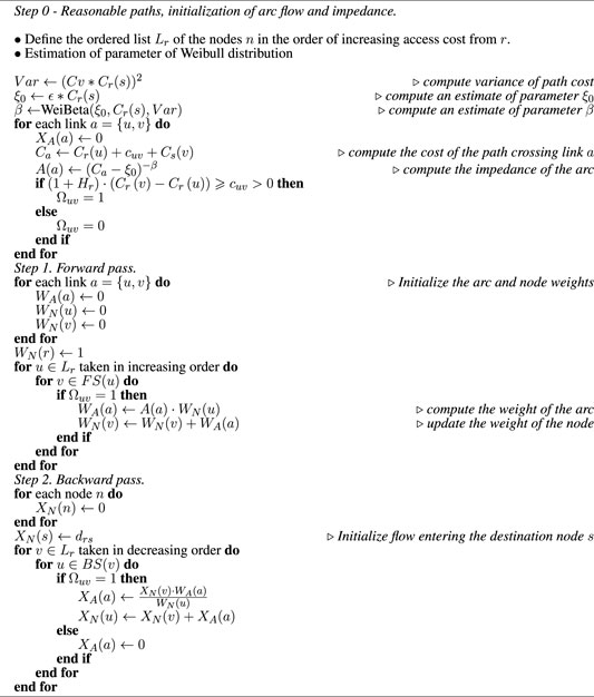
The weibit network loading summarized in Algorithm 2 allows obtaining the arc flow without the explicit path enumeration. In step 0, after the variable initialization and established an origin r and a destination s, the impedance of each arc a is evaluated. Moreover, the belonging of the arc to a reasonable path is evaluated. Step 1 consists of a forward pass where the weight of each arc is calculated. Finally, step 2 consists of a backward pass allowing the calculation of the flow on each arc.

Algorithm 2. Implicit weibit loading procedure.

The path choice models here considered are also used to model congested situations taking into account the variability of costs as described in the following.SUE assignment can effectively be expressed by fixed-point models given by the arc flow function (30) and the arc cost function Eq. 24:

$\mathbf{f}\ast =\mathbf{f}\left(\mathbf{c}\ast ,\mathbf{d}\right)\in S_f(32)$

$\mathbf{c}\ast =\mathbf{c}\left(\mathbf{f}\ast \right)\in \mathbf{c}\left(S_f\right)(33)$

where S_f is the feasible arc flow set.Algorithms based on the method of successive averages (MSA) (Cantarella, 1997) and (Cascetta, 2009) are the most used ones to solve fixed-point models for SUE assignment because they can accommodate any choice model based on random utility theory and are suitable for large-scale applications.Their basic iteration requires the computation of the cost function Eq. 24 to get arc costs from arc flows and the computation of the arc flow function Eq. 30 to get arc flows from arc costs.Applying the MSA leads to the MSA-FA solution algorithm based on the following recursive equation:

${\mathbf{f}}^k={\mathbf{f}}^{k-1}+\alpha \left(\mathbf{f}\left(\right.(\mathbf{c}\left({\mathbf{f}}^{k-1}\right)-{\mathbf{f}}^{k-1}\right).(34)$

Convergence may be proved if the Jacobian of the arc cost function is symmetric (Cantarella, 1997).

4 Experiments

4.1 Application to a Test Network

The first experiment on a test network was carried out with the aim to compare the performance of the considered models in terms of path choice probabilities in a SUN context. The considered network was a 4 × 4 square network, and in order to simplify the interpretation of the results, only one o/d pair was considered. It is depicted in Figure 1, and the characteristics of the arcs are shown in Table 2. Paths for the o/d pair 1001–2016 were considered, and the list of paths is shown in Table 3, where the first six paths in terms of cost are considered. The choice of the number of considered paths derives from considerations on the number of paths potentially used by the users in order to maximize the coverage between the generated and used paths. From literature (e.g., Cascetta et al., 1996), the number of paths was less than 8. Moreover, the analyses reported in (Cascetta et al., 1996) highlight that the use of the first six paths is a reasonable compromise.

FIGURE 1

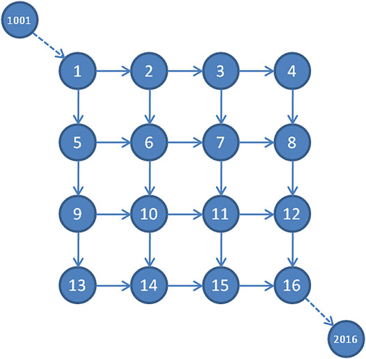
FIGURE 1. Considered test network.

TABLE 2

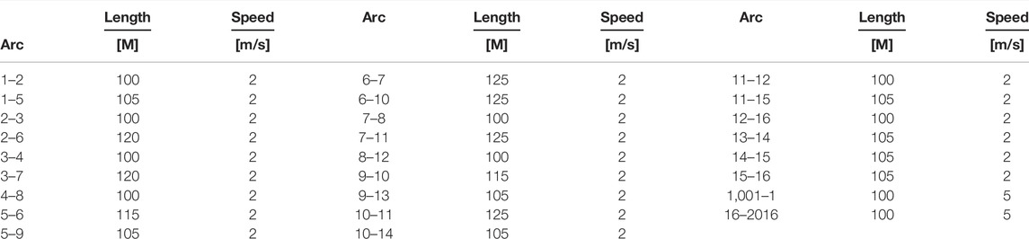
TABLE 2. Characteristics of the arcs of the test network.

TABLE 3

TABLE 3. Considered paths of the test network.

Tests were carried out by considering a set of values for the independent variables above defined for each considered model. Considered values of independent variables are shown in Table 4.

TABLE 4

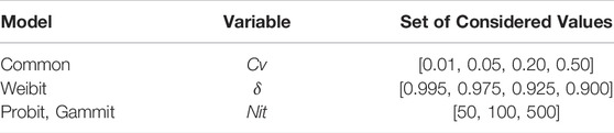
TABLE 4. Considered values of the independent variables.

It is worth noting that Cv is used to compute the variance of: path costs → logit and weibit; arc costs → probit and gammit.

4.1.1 Models With Explicit Path Enumeration

The path set considered in this application is obtained with an explicit path enumeration and a selective approach. Then, among all available paths, the first k ones with respect to the path cost are considered. In this application, we set k = 6. Reported results are at first a comparison among choice probabilities obtained for the shortest path for each of the considered models. Then, the probabilities obtained for each one of the six paths are compared. The explanation of the notation adopted in the figures for the considered model is the following:

- Logit → Logit model.

- WMinyyy → Weibit model where, to estimate β, variance is computed considering the minimum value of path costs and yyy indicates the value of δ (0.995, 0.975, 0.925, and 0.900).

- WMedyyy → Weibit model where, to estimate β, variance is computed considering the mean value of path costs and yyy indicates the value of δ (0.995, 0.975, 0.925, and 0.900).

- Probxxx → Probit model where xxx indicates the number of carried out samples Nit (010, 050, 100, and 500).

- Gamxxx → Gammit model where xxx indicates the number of carried out samples Nit (010, 050, 100, and 500).

Comparing logit with weibit models, as shown in Figure 2, the lower the value of parameter δ is, the closer are weibit models to logit one.

FIGURE 2

FIGURE 2. Path choice probabilities depending on Cv for path 0: Logit vs. Weibit models.

Considering probit and gammit (Figure 3), their behavior is quite similar and a large number of iterations Nit is useful if the variance of costs, that is, the value of Cv, increases.

FIGURE 3

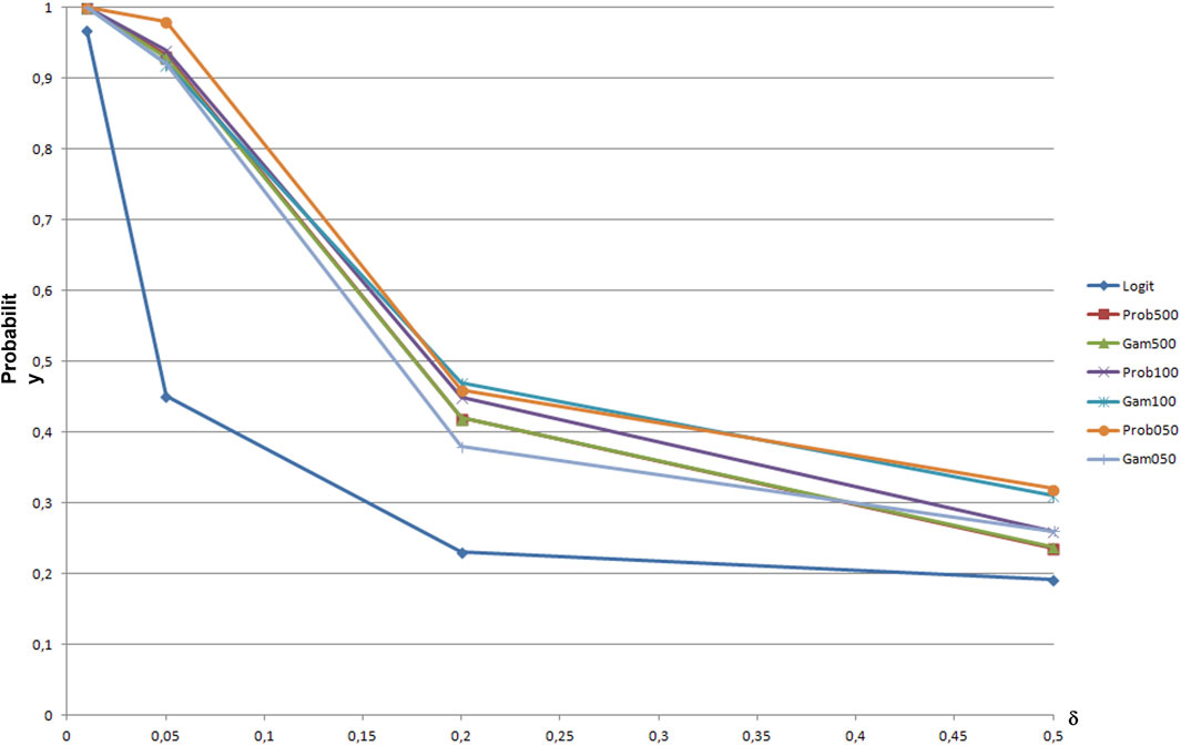
FIGURE 3. Path choice probabilities depending on Cv for path 0: Logit vs. Probit and Gammit models.

In Figure 4 all models are compared considering WeibMed model with δ = 0.995 and gammit and probit with Nit = 500. It can be seen how probit and gammit practically coincide and that the weibit model is quite closer to probit and gammit ones.

FIGURE 4

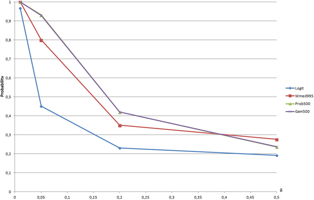
FIGURE 4. Path choice probabilities depending on Cv for path 0: Logit vs. Weibit, Probit, and Gammit best models.

This last comparison has been conducted among all considered paths in Figure 5, and it can be seen that at the increase of variance, differences diminish.

FIGURE 5

FIGURE 5. Path choice probabilities depending on Cv for each path: Logit vs. Weibit, Probit, and Gammit best models.

4.1.2 Weibit Model Without Explicit Path Enumeration

In this case, tests have been carried out by considering a value of δ = 0.995 and the set of variation coefficient Cv = {0.05, 0.20, 0.50}. A first attempt has been conducted to define the value of the cost multiplier H so that the algorithm considered the largest number of arcs in the network and to make a reasonable comparison between explicit and implicit versions of Weibull path choice. For the considered network, a value of H = 0.4 has been considered because, for lower values, only 50% of links result with flows greater than zero, as shown in Figure 6.

FIGURE 6

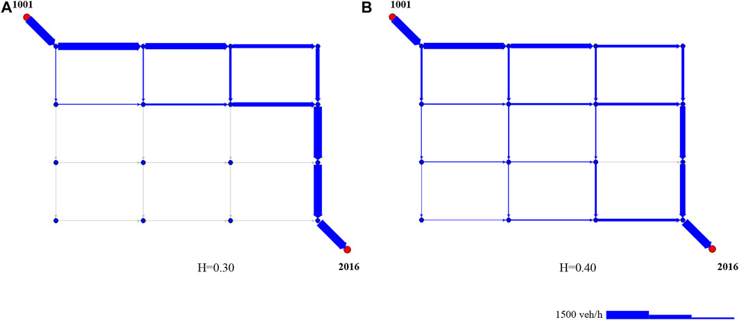
FIGURE 6. Link considered in the implicit loading procedure for values of H =0.30 (A) and H =0.40 (B).

Results are shown by means of a scatter diagram (dots are connected by lines to improve readability) reported in Figure 7, where for each link indicated in the horizontal axis, the values of flows obtained for the two weibit models, with path enumeration (explicit) and without path enumeration (implicit).

FIGURE 7

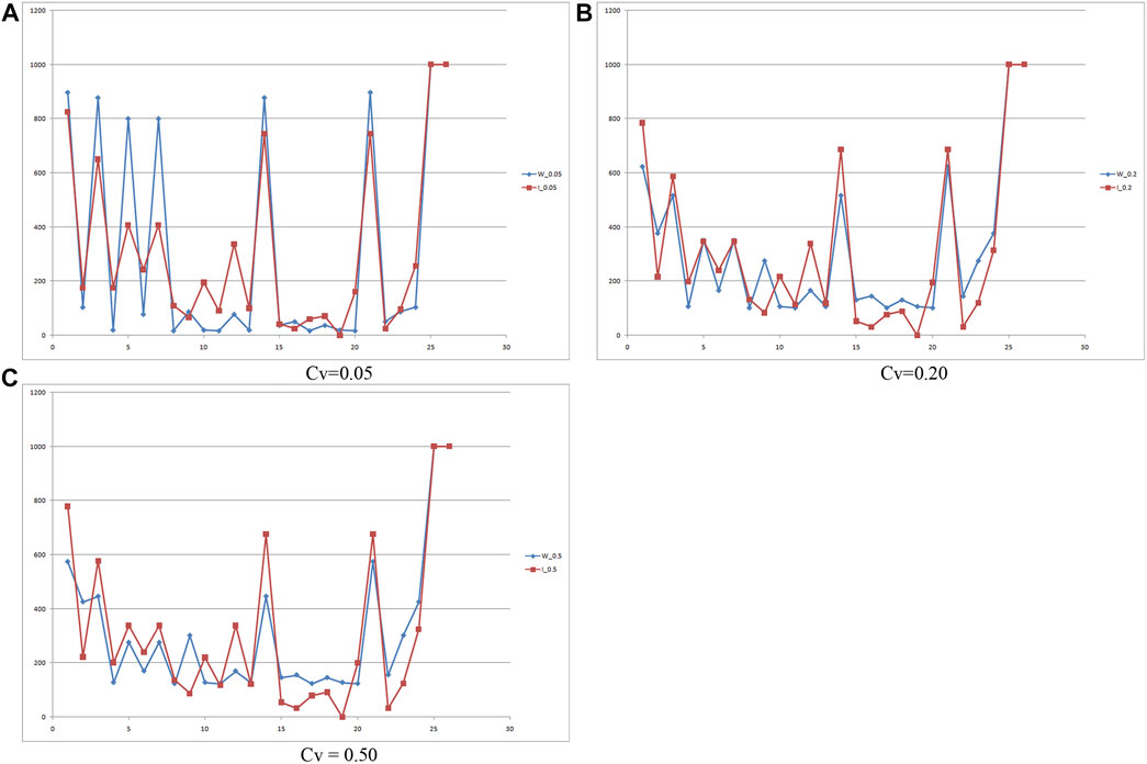
FIGURE 7. Comparison of link flows for values of (A-C) Cv = 0.05, 0.20, 0.50 explicit vs. implicit weibit models.

To compare the values of flows obtained by the explicit Weibit model (f_i) with the implicit one $({\widehat{f}}_i)$, the values of some statistical indicators have been considered: mean squared deviation (MSD), root-mean-square deviation (RMSD), normalized mean-square deviation (NMSD), and normalized root-mean-square deviation (NRMSD).

$MSD=\frac{1}{n}{\mathrm{\Sigma }}_{i=1,n}{\left(f_i-{\widehat{f}}_i\right)}^2(35)$

$RMSD=\sqrt{\frac{1}{n}{\mathrm{\Sigma }}_{i=1,n}{\left(f_i-{\widehat{f}}_i\right)}^2}(36)$

$NMSD=\frac{1}{n}{\mathrm{\Sigma }}_{i=1,n}{\left(\frac{f_i-{\widehat{f}}_i}{f_i}\right)}^2(37)$

$NRMSD=\sqrt{\frac{1}{n}{\mathrm{\Sigma }}_{i=1,n}{\left(\frac{f_i-{\widehat{f}}_i}{f_i}\right)}^2}(38)$

Numerical values are reported in Table 5, where lower values indicate less residual variance.

TABLE 5

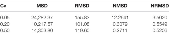
TABLE 5. Comparison of flows explicit weibit vs. implicit weibit.

4.2 Application to a Real Network

This section concerns the comparison of results obtained, in a real context, considering the above-described models applied in a SUE framework in order to explore the capability of reproducing counted flows. Application to a real network allows evaluating model performance on the field by comparing estimated flows with measured ones. Experiments here described have been conducted by considering the road network of Salerno, a town of about 130,000 inhabitants located in southern Italy. The road network has been schematized by means of a graph with 526 nodes and 1,147 arcs connecting 61 internal zones and 13 external ones. Comparisons have been performed by considering observed flows obtained by means of surveys conducted on 69 survey sections. In the adopted stochastic network loading, within the MSA procedure, for those models requiring explicit enumeration of paths, paths have been generated using De la Barra procedure (De La Barra et al., 1993). For each o/d pair, a maximum number of 2,000 iterations have been conducted, considering at most 10 paths not exceeding the 25% of the shortest paths free flow time. Reported results refer to an application considering the values of the independent variables shown in Table 6.

TABLE 6

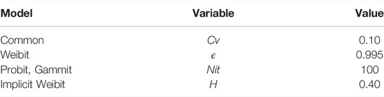
TABLE 6. Considered values of the independent variables in the application to the network of Salerno.

In the MSA-FA algorithm, among the indicators eligible for a stop test (Sheffi, 1985), it has been considered the maximum percentage deviation of flows on arc i, between flow assigned at iteration k $(f_i^k)$ and average flow of previous iteration $({\bar{f}}_i^{k-1})$

$\frac{f_i^k-{\bar{f}}_i^{k-1}}{f_i^k}(39)$

To compare the values of SUE flows obtained by the models (f_i) with the measured ones $({\widehat{f}}_i)$ in the n survey sections, the values of the statistical indicators described in 4.1.2 have been considered. The observed vs. simulated flows reported in Figure 8 summarize the accuracy of the simulation in relation to the type of model used. The goodness of the forecast is represented by any point of the bisector (for which the simulated flow is the same as the observed one). The points on the graph are slightly scattered, and this scattering varies according to the type of model. The goodness of fit is quite high for each model, with values ranging from 0.65 (Logit) to 0.79 (implicit Weibit). Note that the results obtained with probit and gammit are very similar in value.

FIGURE 8

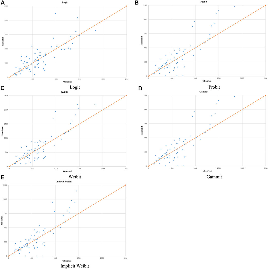
FIGURE 8. Comparison of link flows: observed vs. simulated. (A) Logit (B) Probit (C) Weibit (D) Gammit (E) Implicit Weibit.

Moreover, Table 7 reports, for each model, the frequencies of the bias grouped into intervals with an amplitude of 250 vehicles/h. It emerges that most of the errors are overestimation errors. In particular, the interval 0–500 contains most of the errors with the implicit Weibit that has about 43% of the errors in the interval [0–250) and the Logit that has about 44% of the errors in the interval [250–500). Note that the Logit and the implicit Weibit are the worst in flows underestimation. In this experiment, the worst model in flows overestimation is the Logit model.

TABLE 7

TABLE 7. Bias frequencies (%).

Another graphical analysis (Figure 9) of the obtained results is performed using the Tukey mean-difference plot (also known as Bland–Altman plot), which provides a visual assessment of the shift between two different distributions of values (in this case, between the observed and simulated flows) (Cleveland, 1993). Referring to Figure 9, the y-axis reports the differences (bias) between the observed and simulated flows whereas the x-axis reports the means between such values. The continuous line represents the average value of the bias (Δ), whereas the two dashed lines are the boundaries of the confidence interval. By considering a significance of 95%, the lower limit (l_l) and the upper limit (l_u) are calculated as follows:

$\begin{array}{cc}\hfill l_l=\mathrm{\Delta }-1.96& \cdot \sigma \hfill \\ \hfill l_u=\mathrm{\Delta }+1.96& \cdot \sigma \hfill \end{array}(40)$

FIGURE 9

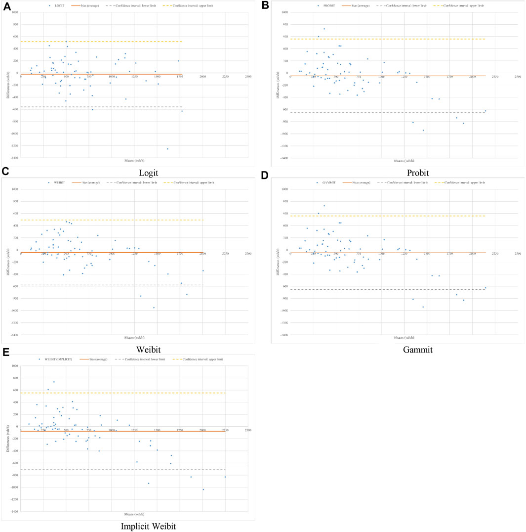
FIGURE 9. Comparison of link flows: Bland–Altman plot.

Considering the logit model (Figure 9A) emerges that the bias ranges from about −1,250 vehicles/h (underestimation) to about 515 vehicles/h (overestimation), although there are errors in under- and overestimation, as discussed above, most of the values fall within the confidence interval (three values are less than l_l). The bias for Probit and Gammit models (Figures 9B,D) presents some points less than l_l and some ones greater than l_u. The weibit model (Figure 9C) suffers from some minor underestimation errors, but most points are within the confidence interval. The implicit weibit (Figure 9E) has values less than l_l and other ones greater than l_u.

The results obtained in terms of NRMSD for each MSA-FA experiment are reported in Table 8 for the considered path choice models, where Iter indicates the number of iteration of the MSA procedure and Time is the time in second needed to carry out the SUE procedure.

TABLE 8

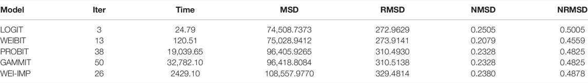
TABLE 8. Results for MSA-FA experiments on a real network of Salerno.

5 Conclusion and Future Developments

Some short comments can be made on the basis of the obtained results. In the Monte Carlo technique, the greater the variance is, the more is the number of samples to be carried out. Practically, a value of Nit = 100 gives acceptable results. Considering the weibit model, a value of parameter δ closer to one (confirming the estimate of the parameter ξ_j, suggested in Castillo et al. (2008)) provides values close to those obtained with models that consider covariance such as probit and gammit, especially in case of a very low variance of path costs. The results obtained with the probit and gammit models practically do not differ from each other considering both the test network and the real one. Considering the minimum path (but also other paths for which it is the same, as shown with regard to the test network in Figure 5), choice probabilities obtained with the weibit model are closer to those obtained with the probit/gammit models than to those obtained with the logit models. About the real network, the best results are obtained by considering the C-weibit model by taking a time that differs by two orders of magnitude from that taken with probit. It is clear that the analysis conducted cannot be considered exhaustive or definitive and that the results, although indicative, also depend on the considered application to reality. The main purpose of this work was to illustrate the hypotheses to be considered for a practical application of the considered models and to provide an example of the results that can be obtained by indicating also an order of magnitude of the bias that can be expected and of the necessary computing resources, in terms of time, considering a standard situation. A study involving other types of models, which is under development, consists of extending a similar analysis taking into account other Logit and Weibit derived models (i.e., path-size logit, C-Logit, mixed Logit, Logit–Probit, and Weibit–Gammit) and QUM. An extension to multitype vehicle assignment to consider autonomous vehicles is also under development.

Data Availability Statement

The original contributions presented in the study are included in the article. Further inquiries can be directed to the corresponding author.

Author Contributions

MDG and AP contributed to the conception and design of the study. MDG performed the statistical analysis and wrote the first draft of the manuscript. MDG and AP wrote sections of the manuscript. All authors contributed to manuscript revision, read, and approved the submitted version.

Conflict of Interest

The authors declare that the research was conducted in the absence of any commercial or financial relationships that could be construed as a potential conflict of interest.

Publisher’s Note

All claims expressed in this article are solely those of the authors and do not necessarily represent those of their affiliated organizations or those of the publisher, the editors, and the reviewers. Any product that may be evaluated in this article or claim that may be made by its manufacturer is not guaranteed or endorsed by the publisher.

Acknowledgments

The authors wish to thank the reviewers for their suggestions, which were most useful in revising the article.

References

Antonisse, R. W., Daly, A. J., and Ben-Akiva, M. (1989). Highway Assignment Method Based on Behavioral Models of Car Drivers’ Route Choice. Transp. Res. Rec. 1220, 1–11.

Google Scholar

Bell, M. G. H. (1995). Alternatives to Dial's Logit Assignment Algorithm. Transp. Res. Part B Methodol. 29, 287–295. doi:10.1016/0191-2615(95)00005-X

CrossRef Full Text | Google Scholar

Ben-Akiva, M., and Bierlaire, M. (1999). “Discrete Choice Methods and Their Applications to Short Term Travel Decisions,” in Handbook of Transportation Science. International Series in Operations Research & Management Science. Editor R. W. Hall (Boston, MA: Springer US), 5–33. doi:10.1007/978-1-4615-5203-1_2

CrossRef Full Text | Google Scholar

Ben-Akiva, M., and Lerman, S. R. (1985). “Discrete Choice Analysis: Theory and Application to Travel Demand,” in Transportation Studies (Cambridge, MA, USA: MIT Press).

Google Scholar

Burrel, J. (1968). “Multiple Route Assignment and its Application to Capacity Restraint,” in Proceedings of the 4th International Symposium on the Theory of Road Traffic Flow (Karlsruhe, Germany: Leutzbach W, Baron P), 229–239.

Google Scholar

Cantarella, G. E. (1997). A General Fixed-Point Approach to Multimode Multi-User Equilibrium Assignment with Elastic Demand. Transp. Sci. 31, 107–128. doi:10.1287/trsc.31.2.107

CrossRef Full Text | Google Scholar

Cantarella, G. E., and Binetti, M. G. (2002). Stochastic Assignment with Gammit Path Choice Models. Transp. Plan. 64, 53–67. doi:10.1007/0-306-48220-7_4

CrossRef Full Text | Google Scholar

Cantarella, G. E., and Fiori, C. (2022). Multi-vehicle Assignment with Elastic Vehicle Choice Behaviour: Fixed-point, Deterministic Process and Stochastic Process Models. Transp. Res. Part C Emerg. Technol. 134, 103429. doi:10.1016/j.trc.2021.103429

CrossRef Full Text | Google Scholar

Cantarella, G. E., Watling, D. P., de Luca, S., and Di Pace, R. (2020). Dynamics and Stochasticity in Transportation Systems. Amsterdam, Netherlands: Elsevier.

Google Scholar

Cascetta, E., Nuzzolo, A., Russo, F., and Vitetta, A. (1996). “A Modified Logit Route Choice Model Overcoming Path Overlapping Problems. Specification and Some Calibration Results for Interurban Networks,” in Proceedings of the Thirteenth International Symposium on Transportation and Traffic Theory (Lyon, France: Lesort, J.B.), 697–711.

Google Scholar

Cascetta, E. (2009). “Transportation Systems Analysis,” in Springer Optimization and its Applications. 2 edn (Boston, MA: Springer US). doi:10.1007/978-0-387-75857-2

CrossRef Full Text | Google Scholar

Castillo, E., Menéndez, J. M., Jiménez, P., and Rivas, A. (2008). Closed Form Expressions for Choice Probabilities in the Weibull Case. Transp. Res. Part B Methodol. 42, 373–380. doi:10.1016/j.trb.2007.08.002

CrossRef Full Text | Google Scholar

Cleveland, W. S. (1993). Visualizing Data. Troy, Ohio: Hobart Press.

Google Scholar

Comi, A., and Polimeni, A. (2022). Estimating Path Choice Models through Floating Car Data. Forecasting 4 (2), 525–537. doi:10.3390/forecast4020029

CrossRef Full Text | Google Scholar

Daganzo, C. F., and Sheffi, Y. (1977). On Stochastic Models of Traffic Assignment. Transp. Sci. 11, 253–274. doi:10.1287/trsc.11.3.253

CrossRef Full Text | Google Scholar

Daganzo, C. F. (1983). Stochastic Network Equilibrium with Multiple Vehicle Types and Asymmetric, Indefinite Link Cost Jacobians. Transp. Sci. 17, 282–300. doi:10.1287/trsc.17.3.282

CrossRef Full Text | Google Scholar

de la Barra, T., Perez, B., and Anez, J. (1993). “Multidimensional Path Search and Assignment,” in PTRC Summer Annual Meeting, 21st, 1993 (Manchester, England: University of Manchester), Vol. P 366, 307–320.

Google Scholar

De Maio, M. L., and Vitetta, A. (2015). Route Choice on Road Transport System: A Fuzzy Approach. Ifs 28, 2015–2027. doi:10.3233/IFS-141375

CrossRef Full Text | Google Scholar

Di Gangi, M., and Vitetta, A. (2018). “Specification and Aggregate Calibration of a Quantum Route Choice Model from Traffic Counts,” in New Trends in Emerging Complex Real Life Problems: ODS, Taormina, Italy, September 10–13, 2018. AIRO Springer Series. Editors P. Daniele, and L. Scrimali (Cham: Springer International Publishing), 227–235. doi:10.1007/978-3-030-00473-6_25

CrossRef Full Text | Google Scholar

Di Gangi, M., Polimeni, A., and Belcore, O. M. (forthcoming). C-Weibit Discrete Choice Model: A Path Based Approach. International Conference on Optimization and Decision Science (ODS2022), Firenze (Italy), August 30-September 2, 2022. Springer.

Google Scholar

Dial, R. B. (1971). A Probabilistic Multipath Traffic Assignment Model Which Obviates Path Enumeration. Transp. Res. 5, 83–111. doi:10.1016/0041-1647(71)90012-8

CrossRef Full Text | Google Scholar

Domencich, T. A., and McFadden, D. (1975). Urban Travel Demand: A Behavioral Analysis. Amsterdam: North-Holland Publishing. Number: Monograph.

Google Scholar

Fosgerau, M., Frejinger, E., and Karlstrom, A. (2013). A Link Based Network Route Choice Model with Unrestricted Choice Set. Transp. Res. Part B Methodol. 56, 70–80. doi:10.1016/j.trb.2013.07.012

CrossRef Full Text | Google Scholar

Leurent, F. (2005). Contributions to the Logit Assignment Model. Transp. Res. Rec. 1493, 207–212.

Google Scholar

Mai, T., Fosgerau, M., and Frejinger, E. (2015). A Nested Recursive Logit Model for Route Choice Analysis. Transp. Res. Part B Methodol. 75, 100–112. doi:10.1016/j.trb.2015.03.015

CrossRef Full Text | Google Scholar

Manski, C. F., and McFadden, D. (1981). Structural Analysis of Discrete Data with Econometric Applications. Cambridge: The MIT Press.

Google Scholar

McFadden, D. (1978). “Modeling the Choice of Residential Location,” in Spatial Interaction Theory and Residential Location. Editors A. Karlqvist, L. Lundqvist, and J. W. Weibull (Amsterdam: North-Holland), 72–77.

Google Scholar

Nuzzolo, A., and Comi, A. (2018). A Subjective Optimal Strategy for Transit Simulation Models. J. Adv. Transp. 2018, 1–10. doi:10.1155/2018/8797328

CrossRef Full Text | Google Scholar

Nuzzolo, A., and Comi, A. (2016). Individual Utility‐based Path Suggestions in Transit Trip Planners. IET Intell. Transp. Syst. 10, 219–226. doi:10.1049/iet-its.2015.0138

CrossRef Full Text | Google Scholar

Prashker, J. N., and Bekhor, S. (2004). Route Choice Models Used in the Stochastic User Equilibrium Problem: A Review. Transp. Rev. 24, 437–463. doi:10.1080/0144164042000181707

CrossRef Full Text | Google Scholar

Prato, C. G. (2009). Route Choice Modeling: Past, Present and Future Research Directions. J. Choice Model. 2, 65–100. doi:10.1016/S1755-5345(13)70005-8

CrossRef Full Text | Google Scholar

Quattrone, A., and Vitetta, A. (2011). Random and Fuzzy Utility Models for Road Route Choice. Transp. Res. Part E Logist. Transp. Rev. 47, 1126–1139. doi:10.1016/j.tre.2011.04.007

CrossRef Full Text | Google Scholar

Rosa, A., and Maher, M. (2002). “Algorithms for Solving the Probit Path-Based Stochastic User Equilibrium Traffic Assignment Problem with One or More User Classes,” in Transportation and Traffic Theory in the 21st Century. Editor M. A. P. Taylor (Bingley, UK: Emerald Group Publishing Limited), 371–392. doi:10.1108/9780585474601-019

CrossRef Full Text | Google Scholar

Russo, F., and Vitetta, A. (2003). An Assignment Model with Modified Logit, Which Obviates Enumeration and Overlapping Problems. Transportation 30, 177–201. doi:10.1023/A:1022598404823

CrossRef Full Text | Google Scholar

Sheffi, Y., and Powell, W. B. (1982). An Algorithm for the Equilibrium Assignment Problem with Random Link Times. Networks 12, 191–207. doi:10.1002/net.3230120209

CrossRef Full Text | Google Scholar

Sheffi, Y. (1985). Urban Transportation Networks: Equilibrium Analysis with Mathematical Programming Methods. Englewood Cliffs, N.J: Prentice-Hall.

Google Scholar

Si, B.-F., Zhong, M., Zhang, H.-Z., and Jin, W.-L. (2010). An Improved Dial's Algorithm for Logit-Based Traffic Assignment within a Directed Acyclic Network. Transp. Plan. Technol. 33, 123–137. doi:10.1080/03081061003643705

CrossRef Full Text | Google Scholar

Vitetta, A. (2016). A Quantum Utility Model for Route Choice in Transport Systems. Travel Behav. Soc. 3, 29–37. doi:10.1016/j.tbs.2015.07.003

CrossRef Full Text | Google Scholar

Wang, J., Peeta, S., and He, X. (2019). Multiclass Traffic Assignment Model for Mixed Traffic Flow of Human-Driven Vehicles and Connected and Autonomous Vehicles. Transp. Res. Part B Methodol. 126, 139–168. doi:10.1016/j.trb.2019.05.022

CrossRef Full Text | Google Scholar

Yai, T., Iwakura, S., and Morichi, S. (1997). Multinomial Probit with Structured Covariance for Route Choice Behavior. Transp. Res. Part B Methodol. 31, 195–207. doi:10.1016/S0191-2615(96)00025-2

CrossRef Full Text | Google Scholar