Ensemble Models of For-Hire Vehicle Trips

Ensemble forecasting is class of modeling approaches that combines different data sources, models of different types, with different assumptions, and/or pattern recognition methods. By comprehensively pooling information from multiple sources, analyzed with different techniques, ensemble models can be more accurate, and can better account for different sources of real-world uncertainties. The share of for-hire vehicle (FHV) trips increased rapidly in recent years. This paper applies ensemble models to predicting for-hire vehicle (FHV) trips in Chicago and New York City, showing that properly applied ensemble models can improve forecast accuracy beyond the best single model.

1 Introduction

The advent of for-hire vehicles (FHVs), such as Uber, Didi, and Lyft is a new occurrence, and the share of FHV in all trips (0.5% in 2017 in the United States (Federal Highway Administration, 2017)) remains low compared to existing modes of transport, but the FHV continues to grow at a rapid rate, and their numbers have already became significant in some areas. Nearly 10% Americans use FHV in any given month in 2017 (Conway et al., 2018); in New York City in particular, the number of FHVs tripled between 2010 and 2019 (Roberton et al., 2020). At this rate of growth, and with the help of autonomous vehicle technology, the FHV will likely become a significant mode of transport, which might cause conflicts with the existing transport system. Empirical research finds FHV to be a significant contributor to traffic congestion (Erhardt et al., 2019), and increases vehicle emission (Roberton et al., 2020), therefore a better understanding of FHV trips is needed.

In addition to conventional models, various machine learning models are increasingly used in transport studies to predict the flow of people (Liu et al., 2021; Ou et al., 2020) and for-hire vehicles (Luo et al., 2020). The current transport modeling practice relies heavily on a single model. When predictions made by alternative models appear not as accurate, even when the performance difference between models were small, these alternative model assumptions are generally discarded. But discarding models that appear to underperform is not a prudent approach to modeling. As McCullagh and Nelder (1989) put it: “Data will often point with almost equal emphasis on several possible models, and it is important that the statistician recognize and accept this.” Model predictions are inherently probabilistic, so relying on a single model assumption is not the best approach.

Our theory of ensemble forecasting (Wu and Levinson, 2021) suggests that there might be room for improvement in both forecast accuracy and reliability by adopting ensemble models. Ensemble forecasting is a modeling approach that combines outputs from different models that use different assumptions or methods of pattern recognition, so that more information can be extracted from available data, and different model assumptions also provide checks and balances for each other. The idea of ensemble forecasting originated in weather forecasting, and has significantly improved forecasting accuracy. There has been very little awareness, and limited use of ensemble models in transport modeling (Wu and Levinson, 2021).

This paper focuses on FHV trips data as proof of concept, and tests the use of different algorithms as base models, and different ensemble models to combine base models in predicting the trip production, attraction, and flow of FHVs between places. The goal is to test whether combining different base models will be able to produce forecasts that are more accurate and reliable, than any individual base model. If ensemble models indeed perform better than the single-model approach, then perhaps prevalent modeling approaches in the four-step transport planning models, at least in the prediction for trip production and attraction can be improved, by the adoption of ensemble models.

2 Data and Methods

2.1 Data

This paper uses For-hire Vehicle (FHV, from ride-hailing companies such as Uber and Lyft) data from New York City and Chicago. On the data side, New York City data includes 239 taxi zones, which provides less training data for models predicting trip production and attraction, when compared to 794 census tracts in the Chicago data; ensemble models for New York City would also have less data to calibrate meta-learners. This smaller data size does not pose a significant issue for predicting flows, as the origin-destination matrix of 2,392 = 57, 121 zone pairs is a sufficiently large number.

Chicago

Data for select For-hire Vehicle trips are available for Chicago (totalling 794 census tracts) (Chicago Data Portal, 2019). This dataset includes trip details such as pick-up and drop-off locations, which can be used to tally the number of trip production, attraction within different zones, and the number of trips between zones.

Trips may begin or end outside the City of Chicago area; these internal-external (or external-internal) trips constitute a small percentage of total trip numbers, and are excluded from the dataset. We extract trips that took place on 26 consecutive Wednesdays in the first half of 2019, and use the average daily trips numbers for models to predict average daily trips.

Explanatory variables include social demographic, and locational factors of a zone. The percentage of non-family households, number of jobs and workers, and the median household income within a zone describe social demographic characteristics of an area. For each location, we include the number of jobs reachable within 30 min via transit as an additional explanatory variable. This “access to jobs” variable characterizes an area in terms of its land use and the provision of public transport. Explanatory variables used in models are listed below.

• 30 min transit access to jobs

• Percentage of households that are not family units

• Median household income

• Number of workers in the area

• Number of jobs in the area

• Size of the area, in sqrkm

• Road distance between origin and destination zone (in the flow model)

New York City

New York City For-hire Vehicle (FHV, rideshare companies such as Uber and Lyft) trips data comes from the NYC Taxi and Limousine Commission (TLC, 2017). The FHV trips data covers the City of New York area, totalling 239 taxi zones.

Trips may begin or end outside the City of New York area; these internal-external (or external-internal) trips presumably constitute a small percentage of total trip numbers, and are excluded from the dataset. We extract trips that took place on 30 consecutive Wednesdays, beginning in the July 2017, for models to predict average daily trips.

Explanatory variables include social demographic, and locational factors of a zone. The list of explanatory variables used for New York City are the same as the ones used in Chicago, but aggregated to New York City taxi zones, which are generally larger than census tracts uses in Chicago. The same “access to jobs” variable used in Chicago is also applied for New York City.

2.2 Models

Conventional modeling method uses a single base model for predictions. We compare the performance of these base models with different ensemble methods that combine base models. This paper uses the R programming language. Packages “neuralnet,”“randomForest,”“gbm” and “rpart” are used for machine learning models, and base R is used for conventional models. The list below shows the category of models used to predict travel demand.

• Base models (Linear, Classification Tree (CT), Random Forest (RF), Gradient Boosting Machine (GBM), Neural Network (NN)¹)

• Simple ensemble models combine outputs from base models. Ensemble models with simple rules use the arithmetic, or the weighted average of different base model predictions as the ensemble model prediction. The simple arithmetic average in particular has been shown to be robust in empirical studies (Winkler, 1989), and often produces better accuracy than using performance-based weights for combining models (Kang, 1986; Elliott, 2011).

• Meta-learner ensemble models (stacking) (Wolpert, 1992) calibrates a higher level model (meta-learner) to combine forecasts made by different base models. Each time, the training data is divided into two parts, with one part used to train the base models, and the other part used to calibrate the meta-learner. To compensate for the reduced size of training data for base models, multiple base models and meta-learners are trained, by repeatedly dividing the training data (e.g. k-fold cross-validation (Chand et al., 2016), k = 3 in this paper). Three types of meta-learners are used, namely the linear, gradient boosting machine, and random forest meta-learners.

• The ensemble of ensembles approach recognizes that ensemble methods combining base models are themselves single algorithms, and therefore have limitations of their own. This method combines different ensemble methods, and is an ensemble of ensembles. The goal is to reduce the dependence on any single one of the ensemble methods. The ensemble of ensembles can be implemented in many different ways; in this paper we use an ensemble of ensembles method that averages outputs from the three meta-learners.

Model performance is evaluated by measuring the difference between predicted and observed values in a separate testing dataset. Both the mean absolute error (MAE) and mean square error (MSE) measure the size of prediction errors, with the MSE focusing more on large errors. Ideally a good model would have low MAE, low MSE, and a small dispersion of prediction errors (standard deviation)

2.3 Trip Production and Attraction

Models predict the average daily number of trips produced and attracted to each of the 794 zones (census tracts) within the City of Chicago area, and each of the 239 taxi zones within New York City, using demographic and locational data as explanatory variables.

We divide the data into training and testing datasets to evaluate the performance of different models. The trip production and attraction zones are divided into two mutually exclusive groups, data in one group is used to train models, and data in the other group is used to test model performance. Generally a zone with many trips previously would continue to have a high trip volume later in time; machine learning models can identify this trend in making predictions and substitute predictions with historical trip numbers, so it would be insufficient to separate training and testing data by time. In this study, the training and testing data are separated spatially, to prevent machine learning models from ‘memorizing’ specific zones. Any zone in the training dataset will not appear again in the testing dataset.

To evaluate the model performance, we repeat the whole process (including splitting the data into training and testing, model calibration and validation) 400 times to obtain a distribution of model performance metrics. All taxi zones in New York City and census tracts in Chicago are divided into two mutually exclusive groups, so data in one group is used to training models, and data in the other group is used for testing model performance.

2.4 Flow Model

Models predict the average daily number of trips between any pair of zones, using descriptive statistics from both the origin and destination zones, and the road distance between the two zones.

Generally the number of trips between two zones are reciprocal, as more trips in one direction often suggest a similar amount of trips in the other direction. So it would not be sufficient to divide training and testing data based on trip pairs alone, for example, including one origin-destination pair in the training data does not exclude trips in the other direction from this origin-destination pair in the testing data. In this study, the entire data is divided into training and testing datasets based on unique trip origins.

We vary the size of training data to test the performance of different models. For each sample size, the model is calibrated on 90 different training samples, and each time applied to 100 testing samples, to obtain a distribution of performance metrics to evaluate model performance.

3 Results

3.1 Trip Production and Attraction

Chicago

Different base and ensemble models have different performance in predicting the average daily number of trips produced from, and attracted to each zone. Figure 1 shows the mean absolute error, and Figure 2 shows the mean square error of different models in predicting trip production. The stability of model performance, as measured by standard deviation of absolute error is shown in Figure 3. Model performance follows identical patterns in predicting trip production and attraction. Figures showing model performance in predicting trip attraction are included in Supplementary Appendix A.

FIGURE 1

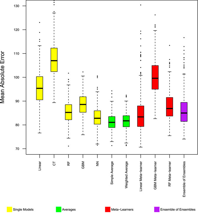
FIGURE 1. Model performance in predicting trip production—Chicago MAE. Distribution of mean absolute error from 400 experiments. Boxes span 25th to 75th percentile, whiskers extend to max/min of the values, excluding outliers (1.5 box heights away from box edges, which are shown as dots).

FIGURE 2

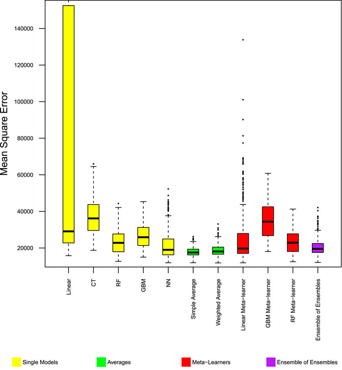
FIGURE 2. Model performance in predicting trip production—Chicago MSE. Distribution of mean square error from 400 experiments. Boxes span 25th to 75th percentile, whiskers extend to max/min of the values, excluding outliers (1.5 box heights away from box edges, which are shown as dots).

FIGURE 3

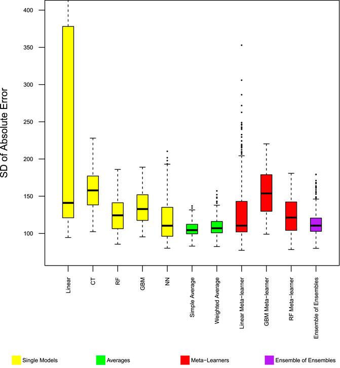
FIGURE 3. Model performance in predicting trip production—Chicago SD absolute error. Distribution of standard deviation of absolute error from 400 experiments.

Among the base models, the linear model has better performance than the classification tree, but has lower performance than other machine learning models. Within the 400 repeated experiments, the linear model has the highest chance to produce large errors.

Ensemble models with simple rules, namely simple average, and weighted average of the base models, improved MAE and MSE beyond the best base model. Figures 1, 2 show these two ensemble models (color coded green) to have the fewest cases where the models have large error measures. In the 400 repeated experiments, these two ensemble models have the most stable performance accuracy between cases, as shown by the standard deviation of absolute error in Figure 3.

Ensemble models with more complex rules, including meta-learners and ensemble of ensembles did not work as well as simple rules ensemble models, and did not significantly improve the mean absolute error of the base models. The linear combination meta-learner and ensemble of ensembles both have lower MSE than the base models. The gradient boosting machine and random forest machine meta-learners provided no noticeable improvement from base models.

New York City

In predicting trip production and attraction in New York City, only the simple average ensemble model is able to improve model performance beyond the best single model (linear). The linear stacking model has similar performance as the best single model. When the classification tree, which has especially low performance in this case, is removed as one of the base models, the simple average of the 4 remaining base models perform better than the best single model (linear) in terms of MAE and MSE, and “no worse” in the stability of model performance. Weighted average ensemble models, and RF, GBM stacking models performed worse than best single model. The ensemble of ensembles method, which averages RF, GBM and linear meta-learners also performed worse than the best single model.

Model performance in predicting trip production is shown in Figures 4, 5, 6. Model performance in predicting trip attraction has identical patter as in predicting trip production, and is shown in Supplementary Appendix A.

FIGURE 4

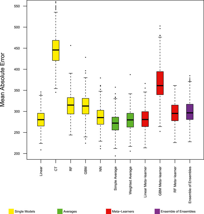
FIGURE 4. Model performance in predicting trip production - NYC MAE. Distribution of mean absolute error from 400 experiments. Base models exclude the classification tree.

FIGURE 5

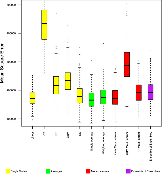
FIGURE 5. Model performance in predicting trip production - NYC MSE. Distribution of mean square error from 400 experiments. Base models exclude the classification tree.

FIGURE 6

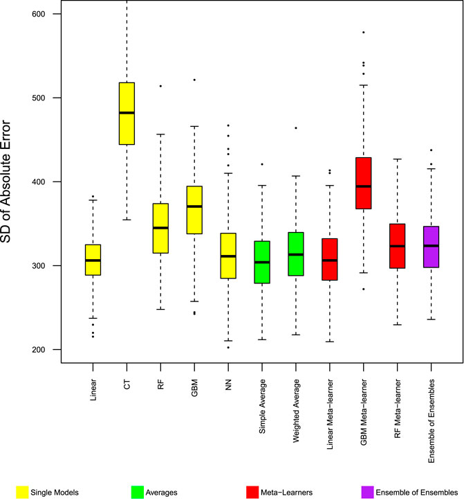
FIGURE 6. Model performance in predicting trip production—NYC SD absolute error. Distribution of SD of absolute error from 400 experiments. Base models exclude the classification tree.

3.2 Flow Model

In predicting the average daily flow of FHV, ensemble models with simple rules provide no improvement from the best single model prediction, but accuracy of these ensemble models are generally similar to the best single model. On the other hand, the weighted average ensemble model scored well (although not the best) on all three measures. The weighted average ensemble model improves forecast accuracy beyond the best single model when the training sample size is small; once the sample size increases, the weighted average becomes less accurate than the best single model prediction.

Model performance in predicting the flow of FHVs is shown in Figure 7 and Figure 8. Among the base models, the gradient boosting machines has the best performance in MAE, MSE, and in the standard deviation of absolute errors. The neural network has good performance in the MAE measure, but very high MSE in predicting flow, suggesting many large errors in neural network predictions. Meta-learner ensemble models (stacking) are able to improve model performance beyond the best single model. Meta-learner ensemble models improved the mean square error beyond the best base model, suggesting a reduction in large errors. Mean absolute error of stacking models is a slight, but not significant, improvement beyond the best base model.

FIGURE 7

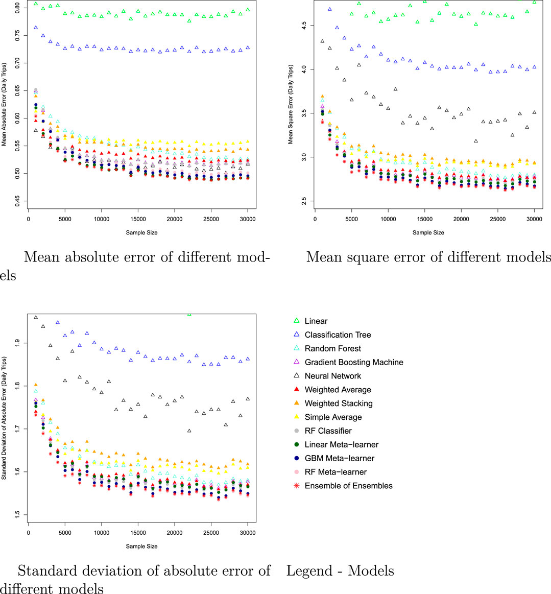
FIGURE 7. Model performance in predicting Chicago FHV flow; Every dot is the average of 90 experiments, each with 100 testing samples.

FIGURE 8

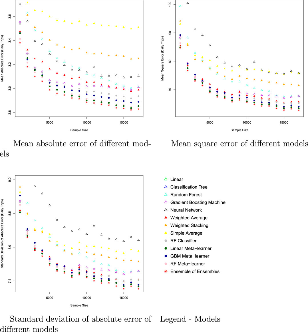
FIGURE 8. Model peformance in predicting New York City FHV flow; Every dot is the average of 90 experiments, each with 100 testing samples.

Among different stacking ensemble models, the linear meta-learner has the best accuracy (MAE and MSE), and produces forecasts with the most stable accuracy. Ensemble of ensembles, averaging three stacking ensemble models (Linear, RF, GBM meta-learners), improves accuracy beyond the best stacking ensemble models.

4 Base Vs. Ensemble Models

How much model performance gain can be achieved from ensemble models is relevant for its potential application. The extent of model accuracy improvement from ensemble models in Chicago are shown in Figure 9; the data in New York city has similar patterns, and is included in Supplementary Appendix B.

FIGURE 9

FIGURE 9. Performance improvement from the best base model—Chicago MAE

With increasing sample sizes, the amount of accuracy improvement provided by ensemble models has diminishing returns, so as sample size grows, each additional unit of data improves the model less. An initial drop in the performance improvement from stacking ensemble models can be observed in Figure 9 for Chicago (and also in New York City), which shows that at certain levels of training data size, the amount of improvement obtainable from ensemble models is reduced. This can be explained by the difference in how fast base models and meta-learners improve their accuracy: if the best base model rapidly improves with more training data, and the meta-learners were to have a slower rate of improvement than the base model, then the gaps between the best base model and the ensemble models will be reduced, resulting in the noticeable kink in the performance improvement. Diminishing returns set in as performance improvement per unit of extra training data drops, and may eventually disappear, in the base models, and the meta-learners are able to further improve upon base models. For this reason, the extent of accuracy improvement with meta-learners generally increases with the size of training data to a point.

On the other hand, if the meta-learner improves faster than the best base model, then the amount of performance improvement from ensemble models will not diminish with more training data, and the kinks in Figure 9 will not appear.

5 Conclusion

This article explores the possibility of improving transport models by adopting ensemble models, by testing ensemble models on For-hire Vehicle (FHV) data, and comparing the performance of ensemble models with the conventional single model approach. The results show that under the right conditions, ensemble models have better performance than the best base model. Since linear models are still widely used for prediction purposes, this paper shows the efficacy of ensemble models, and its potential for wider adoption in transport modeling.

The amount of training data available is a significant factor in the relative performance of ensemble models and base models. In the case of predicting trip production and attraction, with a small training sample size, the simple averages combining rule outperforms other ensemble models and base models, producing both more accurate, and more reliable forecasts. Stacking ensemble rules provide little to no improvement from the best single model. This is possibly because stacking models require sufficient data to be calibrated; with a small sample size, both the base models and meta-learners are not adequately calibrated. We also find the linear meta-learner to have robust performance, in that, although providing no significant improvement, the ensemble models have similar performance to the best single model.

With sufficient data available in predicting FHV flow, meta-learner ensemble models improve model performance beyond the best single model. In most cases the ensemble of ensembles has the best performance. The neural network model has low mean absolute error, but also a significant amount of large errors, which resulted in a high MSE. So reliance on a single model based on one set of performance measure can be risky.

Ensemble models, especially robust ensemble algorithms such as linear meta-learner and the ensemble of ensembles, can generally improve model performance. Ensemble models are also well rounded in performance, providing a good balance between forecast accuracy, large and small errors, and stability of forecast accuracy. In general, ensemble models are either better, or “no worse,” than the best single model forecast. However, discretion is needed in applying ensemble models under different scenarios. In cases without enough data to calibrate models, simpler and robust ensemble models become preferable.

The comparison between ensemble models and the single-model approach shows that, relying on a single model is not the best modeling practice, even when a single model appears to have the best performance; further performance gains can be obtained by combining models with different assumptions or pattern recognition methods. Removing base models with particularly low performance improved the ensemble model. More research is needed to further develop ensemble methods, and to systematically select base models.

Ensembles are more complex than single-models, requiring more effort both in model calibration and interpretation of results. Compared to single models, it is more difficult to explain ensemble model outputs to the general public, or even to people with some technical understanding of modeling. These attributes of ensemble models may have slowed its adoption in transport modeling.

In other disciplines, most notably in the weather forecasting, continuous improvement in modeling methods, and the use of ensemble models (and also better measurement data) have significantly improved forecast accuracy over the years (Blum, 2019). While the single-model approach still has its value in analysis roles, it has outlived its historical role in forecasting. It is time to move on to better modeling methods. Although further tests are needed to evaluate the effectiveness of ensemble models under various circumstances, and to refine ensemble methods under actual use scenarios, we believe ensemble models should be properly recognized and considered as a formal transport modeling approach.

Data Availability Statement

Publicly available datasets were analyzed in this study. This data can be found here: https://www1.nyc.gov/site/tlc/about/tlc-trip-record-data.page.

Author Contributions

HW and DL contributed to conception and design of the study. HW performed the modeling and analysis. HW wrote the first draft of the manuscript. DL reviewed and edited the manuscript. DL supervised the research. All authors contributed to manuscript revision, read, and approved the submitted version.

Conflict of Interest

The authors declare that the research was conducted in the absence of any commercial or financial relationships that could be construed as a potential conflict of interest.

Publisher’s Note

All claims expressed in this article are solely those of the authors and do not necessarily represent those of their affiliated organizations or those of the publisher, the editors, and the reviewers. Any product that may be evaluated in this article, or claim that may be made by its manufacturer, is not guaranteed or endorsed by the publisher.

Supplementary Material

The Supplementary Material for this article can be found online at: https://www.frontiersin.org/articles/10.3389/ffutr.2022.876880/full#supplementary-material

Footnotes

¹Neural Network with a single layer and six neurons.

References

Blum, A. (2019). The Weather Machine: A Journey inside the Forecast. New York City: Ecco.

Google Scholar

Chand, N., Mishra, P., Rama Krishna, C., Shubhakar Pilli, E., and Chandra Govil, M. (2016). “A Comparative Analysis of Svm and its Stacking with Other Classification Algorithm for Intrusion Detection,” in Proceeding of the 2016 International Conference on Advances in Computing, Communication, & Automation (ICACCA)(Spring), Dehradun, India, April 2016 (IEEE), 1–6. doi:10.1109/icacca.2016.7578859

CrossRef Full Text | Google Scholar

Chicago Data Portal, (2019). Transportation Network Providers - Trips. Chicago: City of Chicago. URL Available from: https://data.cityofchicago.org/Transportation/Transportation-Network-Providers-Trips/m6dm-c72p.

Google Scholar

Conway, M., Salon, D., and King, D. (2018). Trends in Taxi Use and the Advent of Ridehailing, 1995-2017: Evidence from the US National Household Travel Survey. Urban Sci. 2 (3), 79. doi:10.3390/urbansci2030079

CrossRef Full Text | Google Scholar

Elliott, G. (2011). Averaging and the Optimal Combination of Forecasts. San Diego: Manuscript, Department of Economics, UCSD.

Google Scholar

Erhardt, G. D., Roy, S., Cooper, D., Sana, B., Chen, M., and Castiglione, J. (2019). Do transportation Network Companies Decrease or Increase Congestion? Sci. Adv. 5 (5), eaau2670. doi:10.1126/sciadv.aau2670

PubMed Abstract | CrossRef Full Text | Google Scholar

Federal Highway Administration (2017). 2017 National Household Travel Survey (NHTS).

Google Scholar

Kang, H. (1986). Unstable Weights in the Combination of Forecasts. Manag. Sci. 32 (6), 683–695. doi:10.1287/mnsc.32.6.683

CrossRef Full Text | Google Scholar

Liu, C. H., Piao, C., Ma, X., Yuan, Y., Tang, J., Wang, G., et al. (2021). “Modeling Citywide Crowd Flows Using Attentive Convolutional Lstm,” in Proceeding of the 2021 IEEE 37th International Conference on Data Engineering (ICDE), Chania, Greece, April 2021 (IEEE), 217–228. doi:10.1109/icde51399.2021.00026

CrossRef Full Text | Google Scholar

Luo, W., Zhang, H., Yang, X., Lin, B., Yang, X., Zang, L., et al. (2020). “Dynamic Heterogeneous Graph Neural Network for Real-Time Event Prediction,” in Proceedings of the 26th ACM SIGKDD International Conference on Knowledge Discovery & Data Mining, August 2020, 3213–3223. doi:10.1145/3394486.3403373

CrossRef Full Text | Google Scholar

McCullagh, P., and Nelder, J. (1989). Generalized Linear Models.

Google Scholar

Ou, J., Sun, J., Zhu, Y., Jin, H., Liu, Y., Zhang, F., et al. (2020). “Stp-trellisnets: Spatial-Temporal Parallel Trellisnets for Metro Station Passenger Flow Prediction,” in Proceedings of the 29th ACM International Conference on Information & Knowledge Management, October 2020, 1185–1194. doi:10.1145/3340531.3411874

CrossRef Full Text | Google Scholar

Roberton, J., Schmidt, S., and Stiles, R. (2020). Emissions from the Taxi and For-Hire Vehicle Transportation Sector in New York City.

Google Scholar

TLC (2017). New York City FHV Trip Record Data. New York City: NYC Taxi and Limousine Commission. URL Available from: https://www1.nyc.gov/site/tlc/about/tlc-trip-record-data.page.

Google Scholar

Winkler, R. L. (1989). Combining Forecasts: A Philosophical Basis and Some Current Issues. Int. J. Forecast. 5 (4), 605–609. doi:10.1016/0169-2070(89)90018-6

CrossRef Full Text | Google Scholar

Wolpert, D. H. (1992). Stacked Generalization. Neural Networks 5 (2), 241–259. doi:10.1016/s0893-6080(05)80023-1

CrossRef Full Text | Google Scholar

Wu, H., and Levinson, D. (2021). The Ensemble Approach to Forecasting: A Review and Synthesis. Transportation Res. C: Emerging Tech. 132, 103357. doi:10.1016/j.trc.2021.103357

CrossRef Full Text | Google Scholar