 Arslan Ali Syed
 Florian Dandl
 Bernd Kaltenhäuser
 Klaus Bogenberger
94% of researchers rate our articles as excellent or good
Learn more about the work of our research integrity team to safeguard the quality of each article we publish.
Find out more
METHODS article
Front. Future Transp., 14 June 2021
Sec. Transportation Systems Modeling
Volume 2 - 2021 | https://doi.org/10.3389/ffutr.2021.681451
Ride hailing (RH) services have become a common mode of transportation in the last decade. Usually, statistical tools are used to improve their performance, whereby the tools typically divide the whole operational area into multiple regions. These tools usually assume that the regions are independent of each other even though vehicles from one region can be used to serve neighboring regions, thereby a method is required that consistently relates vehicle demand and supply between geographically neighboring regions or to the whole operating area. This hinders tapping into the full potential of region-based performance improvement techniques like the repositioning of idle vehicles. Therefore, we develop an innovative reachability function-based method that coherently builds a relation among all regions in the form of a spatial density of the measured quantity. We use it to calculate the differences of vehicle supply and demand for the whole operational area in the form of an imbalance density. Based on this, we derive a novel repositioning formulation that significantly reduces both the overall vehicle imbalances and the total distance of repositioning trips, and thus improves the long-term RH performance. We test the approach in an agent-based simulation for an RH scenario with automated vehicles, using open-source New York City taxi data as demand. The approach shows a remarkable improvement over the state of the art repositioning strategies that balance the fleet over the individual regions. Furthermore, we introduce kernel-based key performance indicators (KPIs) that can be calculated at the time of making repositioning decisions. We also show the correlation of the KPIs with long-term performance gains. We expect that these KPIs can benefit future statistical (machine learning) approaches for repositioning.
In the last decade, the widespread usage of smartphones coupled with the availability of high-speed mobile internet has led to many new and innovative use cases. Among these applications, the emergence of private-sector mobility service providers (MSPs)—also known as transportation network companies (TNCs) like Uber, Lyft, and DiDi—is a major development in how people interact with transportation networks.
Competitive prices, ease of transport, and seamless steps from requesting a ride to the final payment has caused wide-spread acceptance and large-scale usage of MSPs for regular trips. Especially in areas with a poor public transport system, these services represent a viable alternative to private vehicles. However, the easy to use apps and public availability of MSP vehicles has significantly induced additional demand contributing to an increase of vehicle kilometers traveled (VKT) and possibly an increase in congestion (Henao and Marshall, 2019; Kaltenhäuser et al., 2020). To reduce the overall VKT, spatially and temporally overlapping customers can be combined into single trips, i.e., shared-ride Mobility on Demand (MOD), which could be strengthened by regulation (Dandl et al., 2021). However, non-shared rides still contribute the most in current MOD services (Henao and Marshall, 2019; Hyland and Mahmassani, 2020). We also focus on a non-shared MOD service model and refer to it as a ride hailing (RH) service in the current contribution.
With the increasing share of MSPs for passenger transportation, there is also a significant growth in the scientific literature for improving their efficiency. The majority of these studies focuses on improving the aspect of online matching or the dynamic assignment of vehicles to customer requests. Simulation studies compare various dynamic assignment strategies to improve the overall service quality and profit of the MSPs. Some of them also utilize the repositioning of idle vehicles to vehicle-deficient regions to increase the number of served customers; this process is also denoted by rebalancing or relocation in the literature. In the current work, we use the words zones and regions interchangeably for a disjoint set cover of the whole operation area.
The periodic repositioning of idle vehicles to appropriate regions generally increases the number of total customers served at the expense of empty VKT (Dandl et al., 2019). It requires the selection of idle vehicles and their respective destinations. Generally, repositioning methods do not integrate the granularity level of raw coordinates because 1) it makes the solution space intractable and 2) forecasts of supply and demand are not available at this resolution. Hence, the general approach is to divide the city into various regions and make repositioning decisions according to forecasts for these regions. However, many region-based repositioning methods do not consider spatial proximity of the regions when comparing forecasts of demand and supply. Because a customer in a region without vehicles can also be picked up by a vehicle from a surrounding region it might not be necessary to equalize the demand and supply imbalance in each individual region, but consider a bigger picture and the relations of regions depending on the sizes of regions and the acceptable user waiting time. Although some works indirectly considered inter-regional relations with reinforcement learning (RL) strategies, an explicit relationship based on inter-regional distances is still lacking (Mao et al., 2020). More importantly, a clear-cut optimization formulation is needed that consistently considers the impact of a repositioning decision on the destination region as well as on its surrounding regions.
Therefore, the primary purpose of this study is to develop a general repositioning procedure that coherently looks at the spatio-temporal vehicle-demand imbalances of regions considering their respective surrounding regions. We introduce a novel heat-map or kernel density estimation (KDE)-based repositioning strategy that considers the impact of repositioning decisions on the regions idle vehicles originate from and drive to as well as their surrounding regions. Even though we study the developed repositioning approach on the RH scenario with autonomous vehicles (AVs), the fundamental procedure of using KDE is general and can be applied to other MOD service models as well.
The rest of the paper is structured as follows. The next section presents the necessary background and literature review of the dynamic assignment problem along with a brief delineation of current work. Then, Section 2 presents details of the studied MOD mode and associated repositioning problem. Section 3 describes the adoption of KDE for the density-based repositioning method and the related computational complexity when used for general repositioning without regions. Afterward, we present a computationally feasible procedure to the above method using regions. Subsequently, Section 4 shows the numerical experiments used to evaluate the effectiveness of the presented repositioning approach. The last section then presents the summary, limitations, and possible future directions.
The core operational problem for MODs is part of the class of stochastic dynamic vehicle routing problems (SDVRP), or more specifically it is related to the well known multi-depot dynamic dial-a-ride problem (D-DARP), where the current location of a vehicle can be assumed to be the depot for that specific vehicle (Agatz et al., 2012; Toth and Vigo, 2014). Commonly, studies use rolling horizon strategies which are also referred to as batching to deal with the dynamic aspect of SDVRP. The requests are temporally accumulated for specific time periods and then the same methods as used for the static problems (where all the customer requests are known in advance) are applied. Therefore, there is a growing interest in operations research for both static and dynamic variants of DARP (Ho et al., 2018).
Generally, research dealing directly with the SDARP focused on comparatively small sized artificial data with a significantly large time horizon for acceptance or rejection of a request. The large time horizon exponentially increases the number of possible combinations, making the problem much more difficult to solve. MOD services in large cities deal with thousands of vehicles and customers, but the time window for replying to a customer is considerably short and customers do not accept long waiting times. This highly dynamic behavior of MOD services makes the assignment problem much easier to solve than a traditional multi-depot SDARP, allowing significant pruning of the search space for the MOD assignment problem.
A significant number of works used the above observation for simulating MOD scenarios with actual data. Hyland and Mahmassani (2018) and Maciejewski et al. (2016) studied various batch-based assignment strategies for vehicle assignment. Alonso-Mora et al. (2017a) presented an interesting general approach for a large scale ride sharing (RS) scenario inside Manhattan using open source New York City (NYC) taxi data with a 30 s batching period. They explicitly pruned the search space by first developing a graph of possible trips and then solving a set cover problem for assigning trips to vehicles. Engelhardt et al. (2019) developed a similar algorithmic approach for a shared ride scenario with lower demand densities on a larger operating area in Munich, Germany. Some other researchers tried using DARP metaheuristic approaches for dynamic simulation of real data (Syed et al., 2019b; Erdmann et al., 2019).
It is generally known from operations research literature that including statistical information inside the dynamic problem significantly improves the overall solution quality (Toth and Vigo, 2014). We see a growing interest of using past experiences to improve the overall MOD performance. Two general approaches in this regard are 1) explicitly using modern machine learning (ML) techniques and 2) specific rule-based incorporation of the statistical information. The ML-based approaches are still comparatively new to the field. Works by Nazari et al. (2018), Hamzehi et al. (2019) tried to solve the basic assignment problem using reinforcement learning (RL) while (Syed et al., 2019a; Hottung and Tierney, 2019) improved ALNS using ML methods. Al-Kanj et al. (2020) developed a dynamic programming approach for a combined dispatch, recharge, and repositioning problem and tested it on a regular grid inside New Jersey. Mao et al. (2020) presented an RL-based approach for the repositioning problem inside Manhattan using NYC taxi data and NYC taxi zones as repositioning regions. They showed that the trained RL agent produced results within analytical upper and lower bounds of the optimal solution. However, both Al-Kanj et al. (2020) and Mao et al. (2020) used a simplified customer-vehicle assignment due to a very low temporal resolution of 15 min. Besides, these approaches require thousands of iterations in order to learn a good policy which makes it difficult to directly adopt bigger agent-based simulations with thousands of requests and small time steps.
Due to the rule-based utilization of statistical information, a majority of works used the repositioning or efficient routing of vehicles. Usually the objectives include either serving more customers or increasing the overall profit with the least possible increase in VKT. One strategy is to use short-term forecasts alongside the batch assignment problem to move idle vehicles to demand-intensive regions (Sayarshad and Chow, 2017; Dandl et al., 2019) or to maneuver the en-route vehicles in RS through regions expecting new customers (Alonso-Mora et al., 2017b). Repositioning aims at moving idle vehicles from areas where no demand is expected to areas where vehicles are likely needed. The idea is the same as relocation in carsharing systems (Weikl and Bogenberger, 2013; Weikl and Bogenberger, 2015), but do not require staff and are therefore much cheaper and frequent. RH studies periodically solve repositioning problems that are completely separate from the batch optimization (Pavone et al., 2012; Fagnant et al., 2015; Dandl and Bogenberger, 2019; Winter et al., 2020). They solve an optimization problem to determine the number of idle vehicles that needs to be repositioned from one region to another. To solve a single instance of the problem, some of the works use heuristics to distribute the vehicles to neighboring zones (Fagnant and Kockelman, 2014), while the majority use some commercial solver to solve discrete optimization problems (Alonso-Mora et al., 2017a; Wallar et al., 2018; Dandl and Bogenberger, 2019). The objective function generally includes a combination of repositioning VKT and a measure of regional imbalances.
Whether the repositioning is done alongside the batch optimization or completely separately, most of the repositioning formulations do not consider the size and proximity of the regions to determine the imbalance in the system. This leads to two major issues:
• Region-based repositioning algorithms try to balance as many regions as possible with minimum extra VKT (Pavone et al., 2012) or balance adjacent regions (Fagnant and Kockelman, 2014), while ignoring the fact that for many smaller regions a vehicle from the neighboring regions can be assigned to the customer. As shown in Figure 1, many smaller regions in the center and the lower town could be balanced by sending vehicles to only some of the regions. Instead, the algorithms tried to balance all regions independently, irrespective of proximity.
• As a consequence of the above point, short repositioning trips are prioritized, which can lead to larger areas (such as the Upper West Side and Upper East Side in Figure 1) remaining highly imbalanced although idle vehicles could have been repositioned there.
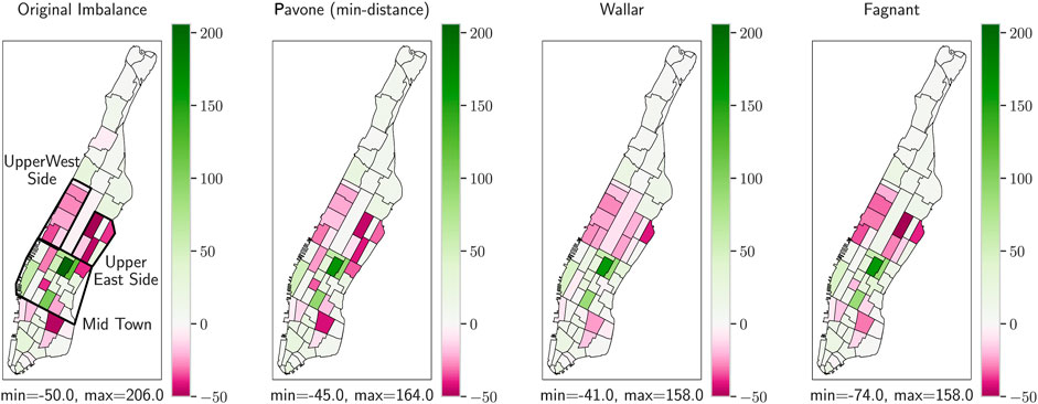
FIGURE 1. An instance of the mid-term repositioning inside Manhattan, New York City using methods of Pavone et al. (2012), Wallar et al. (2018), and Fagnant and Kockelman (2014). The positive values represent taxi zones with surplus of vehicles while negative values correspond to zones with a deficiency of vehicles. The algorithms treated each zone independently and preferred repositioning to zones around the surplus zones while leaving the areas in the upper west and east sides highly deficient.
Perhaps some of the ML-based repositioning works by Al-Kanj et al. (2020), Mao et al. (2020) could be said to have implicitly considered the above observations. However, the exact regional relationships and why they are built during the training process remain unclear. Combined request-assignment and repositioning approaches (Sayarshad and Chow, 2017; Hyland et al., 2019) consider the assignment to nearby regions explicitly. However, it is possible that operators might want to keep request assignment and repositioning separate as they have very different dynamics: requests require immediate actions whereas forecasts of demand and supply for a longer time horizon evolve much slower over time. In a separate repositioning approach, Pouls et al. (2020) introduced a binary reachability parameter, which is 1 if a vehicle from one region can reach another region within a maximum waiting time.
We use a concept partially similar to Pouls et al. (2020), but instead of time-based reachability, we use distance-based reachability to introduce a 2D vehicle density function. The function consistently models inter-regional relationships while considering the sizes and proximity of individual regions and resolves both of the above issues. It uses ideas from KDE to better model distance-based inter-regional relationships than spatially independent zones. The general nature and simple formulation of the density term provides the major advantage of linking any regional measurement that is expected to affect other regions and the overall operational area; thus, it can significantly improve the performance of any future MOD contribution that uses measurements based on inter-regional relations.
Second, we apply the density term to the repositioning of idle vehicles in the MOD services. First, the regional vehicle imbalances are measured using customer forecasts and the available idle vehicles. A positive or negative regional weight is assigned according to the surplus or deficiency of vehicles, respectively. Next, a 2D linear kernel or vehicle reachability function (VRF), representing the area from which a vehicle at the center of the region can pick up a customer, is used as the reachability function inside the above mentioned density method. Then, we formulate a multi-objective repositioning problem, where the importance of the imbalance density has to be optimized against the repositioning VKT. This whole procedure is analogous to the balancing of weights inside a weighted KDE, where the imbalance density can be looked at as a 2D heat-map of the vehicle imbalance.
Finally, the repositioning approach presented can pave the way for more advanced operational strategies. Even though we use pre-defined regions for computational efficiency, the method will probably show its full potential with a more refined forecast granularity and artificial intelligence (AI)-based algorithms. The introduced instant repositioning rewards are likely to help AI-based (and non-myopic dynamic programming) algorithms because it is generally difficult to evaluate the long-term effectiveness of repositioning decisions at a given time. Therefore, we present the correlations of served customers and density-based KPIs which can be used as indicators of long-term rewards in an AI-based algorithm.
We compare the performance with multiple methods to study the benefits of the developed repositioning methods. Since there is no comprehensive study comparing the performance of major repositioning strategies on the NYC dataset, we resorted to our own testing of multiple methods. Due to the required implementation effort and the number of iterations required for training, it is difficult to compare against dynamic programming and RL-based methods. Therefore, the first method chosen is the min-distance approach by Pavone et al. (2012). It was originally named the adaptive real-time rebalancing policy by Pavone et al. (2012) and aims at equally distributing excess vehicles among regions with minimal repositioning VKT. The second method by Wallar et al. (2018) maximizes the number of customers received by repositioned vehicles after reaching the destination zone. We also test the commonly used heuristic method of Fagnant and Kockelman (2014) which tries to balance the expected demand and idle vehicles in the neighboring zones. The dynamic simulation experiments of min-distance performed significantly better than the other two methods. For presentation purposes, the current paper only includes the results of the min-distance method, and the descriptions and comparisons with all methods are attached as Supplementary Material.
This section presents the formal definitions, assumptions, and the dynamic MOD service problems focused on in the current study.
The studied RH service has the following characteristics:
• Each customer i dynamically requests a ride at time
• A customer can only be picked up within the maximum waiting time,
• Any customer that cannot be picked up before
• A customer pick-up delay is defined as the difference between the actual arrival time of the vehicle at
• The fleet consists of homogeneous AVs that do not need recharging or refueling.
• The assignment of vehicles to customers is controlled by a central fleet controller (FC).
• A fleet of fixed size n.
• Only a single customer request can be served at a time.
The dynamic setting means that at time t, the FC is not aware of requests i with
The FC in a dynamic setting tries to get as close as possible to the static optimal solution by proactively sending vehicles to regions where higher customer demands are expected rather than assigning it to an explicitly known customer demand. Therefore, we define two problems that the FC should address: the vehicle assignment problem, where vehicles are assigned routes that include picking-up and dropping-off requests, and the vehicle repositioning problem, where vehicles are moved within the operating area based on expected demand. As expected demand is stochastic, assignments to explicit customer requests are typically prioritized.
Figure 2 illustrates the dynamism related to the control of the MOD fleet. Based on the vehicle states (positions, on-board customers, and assigned routes), the set of known requests, and the forecasts of future demand, the FC tries to find optimal solutions to the vehicle assignment and repositioning problems, and plans vehicle routes. The vehicles follow these plans until the control process is performed again.
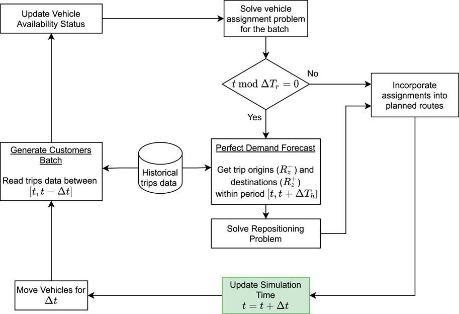
FIGURE 2. Dynamic fleet control for a MOD service.
The overall performance or effectiveness of a specific strategy can only be evaluated after all the customer requests are received. Therefore, we quantify the service quality in terms of total monetary profit based on traveled distances as overall objective of the dynamic RH scenario. We study a system, in which every served customer i must pay a fixed cost ζ and a variable cost of
With the above definitions, for a set of all the served customer requests
where
We batch the new requests for 30 s before assigning them to the vehicles. The FC solves an optimization problem on the batched requests, which we refer to as vehicle control optimization (VCO). Since the superordinate problem is dynamic and the overall objective of the FC is to maximize the profit in Eq. 1, the objective function in VCO can be different from Eq. 1 with additional terms for statistical data. However, we keep the objective in VCO the same as the actual profit for the sake of simplicity. Thus, the batch optimization problem is described as follows.
The FC first checks for the availability of the vehicles, i.e., the time and the position when and where a vehicle could be assigned a new task. If the vehicle is already serving some customers, then it finds the drop-off time and location of the last customer in the vehicle’s path (Hyland and Mahmassani, 2018). Then the VCO maximizes Eq. 1 for the batched requests
• Each request is served at most by one vehicle.
• At most one pick-up is assigned to each vehicle.
• For a served request i the pick-up time is before
We assume that any request that could not be matched with a vehicle in the current batch, will be most likely not matched in the future batches as well. Since vehicles en-route to drop off customers are viewed as available, this assumption would be invalid only if another customer was both picked up and dropped off within this time frame and the respective vehicle would be very close to the request’s pick-up location. For simplicity, all the unassigned requests are immediately rejected and removed from future batches.
In a dynamic MOD scenario, the spatio-temporal distributions of customer demand and vehicle availability play a major role in improving the overall service quality. After dropping off a customer, vehicles might wait a long time before getting another customer, despite the fact that there are many unserved customers in other parts of the city. Therefore, a general repositioning problem tries to minimize this supply and demand gap by routing the idle vehicles to areas with expected vehicle deficit. Ideally, a repositioning algorithm should consider every possible coordinate inside the city for this purpose. However, demand (and for larger forecast horizons, supply as well) forecasts are usually not available on such a fine granularity, and dealing with an algorithm on such a level poses a significant computational challenge.
Typically, vehicle supply and demand are forecast for discrete regions or zones within the operational area. The region-based approach also limits the possible destinations of repositioning vehicles. Let Z denote a disjoint set of regions in the operating area. As shown in Figure 2, the FC periodically calls its repositioning algorithm after every
Let t be the simulation time when the repositioning algorithm is performed. First, the supply and demand are forecast in each zone for a temporal horizon
Next, the FC calculates the regional supply-demand imbalance weights
Let surplus zones
Based on the zone-based solution
It should be noted that most region-based repositioning algorithms assume that a single repositioned vehicle changes the weight imbalance by one:
where
The subsequent section derives a vehicle density-based repositioning method for calculating the flow matrix
This section presents the solution approaches used in the current study. It starts with a brief description of the KDE and how it is modified to obtain a density term for MOD services. Then it uses the density term for the repositioning of idle vehicles. Finally, it introduces KDE-based KPIs to evaluate repositioning assignments.
KDE is a well known non-parametric probability density function (pdf) estimator first introduced by Parzen (1962), Chen (2017). KDE tries to automatically adopt itself to the shape of the underlying density function. If
where
There are many smooth kernels that are generally used in KDE, e.g., triangular, Gaussian, triweight, etc. However, we interpret the kernel function in terms of an approximation to the maximum reachable distance by a single vehicle. Any vehicle located at the center of the kernel will have the highest probability of serving a customer at the center, that will become smaller as the Euclidean distance of the customer pick-up location increases. Thus, in this study we use the simple triangular function, given as:
We use the Euclidean norm in the above equation, i.e.,
The fundamental usage of KDE is to estimate the underlying pdf of a dataset without any assumption that the pdf belongs to a parametric family. KDE adopts the shape of the estimated pdf directly from the data, making it a very useful tool for data drawn from complicated distributions. The most important parameter of a KDE, i.e., h, is usually calculated automatically using various approaches to reduce the asymptotic mean integrated square error (AMISE). The data are center and the overall spread of the estimated pdf is heavily dependent on the choice of bandwidth h (the spread of a single data point) (Grodzevich and Romanko, 2006).
The motivation of using a KDE-inspired approach for the repositioning problem is to balance the distribution of available vehicles (supply) according to the customer distribution (demand), such that the maximum number of customers could be served with least VKT. KDE seamlessly combines the impacts of neighboring data points through kernels. Since the bandwidth h defines the spread of the kernel function, we can interpret it as an approximation of the maximum reachable (servable) distance of a single vehicle (customer request). Similarly, we can refer to the kernel function as reachability (servability) function for the vehicles (customer requests). This naturally eliminates the fundamental limitation of region-based repositioning approaches that treat each region separately without due regard to the proximity of other regions. However, using the above mentioned KDE formulation and approach directly leads to some major inconsistencies as described below:
1. The major focus of bandwidth selection algorithms in KDE is to find a h that would improve the estimate of the underlying probability density function of the random variable. Thus, in the case of customer and vehicle geographical locations, it would only mean to estimate a h that would provide a good estimate of the probability density for generating the customer and vehicle locations. Such a h would not correspond with our interpretation of h as the reachable distance of the vehicle.
2. The customer and vehicle data in an RH scenario are dynamic and thus the underlying density of their location is expected to change in every repositioning throughout the day and week and thus, the value of h derived from bandwidth estimation algorithms can vary significantly, which may lead to long-term inconsistent decisions.
3. Even for a single instance of the repositioning problem, the values of bandwidth h obtained from an algorithm might be significantly different for the customer and vehicle distributions. Thus, even if we reposition idle vehicles to close the gap between the customer and vehicles KDE, the repositioned vehicles still may not serve the intended customer because of different bandwidths. For example, consider the case when customers’ and vehicles’ KDE have bandwidths of 500 m and 2 km, respectively. The algorithm will falsely reposition very few vehicles assuming that the vehicles have a reachability of 2 km, which may not be applicable due to the average speed in the area of operation.
4. Since the KDE is normalized with the number of available data points (Eq. 4) to make the integral unity, the scales of customers and vehicles KDE might be significantly different. For example, consider a case with 100 expected customers and 300 idle vehicles with KDEs calculated using Eq. 4. The algorithm would try to unnecessarily send a high number of vehicles close to the expected customers, as the customers KDE would be on a similar scale as the idle vehicles KDE due to normalization.
To resolve issues 1 and 2, instead of using a data-driven value of h calculated through bandwidth estimation algorithms, we select h according to the network state (size of the operating area, average speed, etc.) and RH service quality (maximum waiting time). For issue 3, we notice that a major problem is caused by normalization of the KDE on the same scale such that
where k is the triangular kernel given in Eq. 6. The above equation does not represent a pdf, however, it has a useful property of
If individual points are aggregated in a set of points
with
Ideally, density-based repositioning should use raw coordinates of forecast customers in Eq. 7 to distribute the idle vehicles. However, such a repositioning method would not be computationally feasible even if the exact locations of the future customers are known (see Supplementary Material for a more elaborate discussion). Therefore, this section derives a reachability function-based repositioning with regions (RFRR) approach based on Eq. 8. The derived RFRR formulation is also applicable to any regional forms, e.g., predefined equidistant bins. However, we use the centroids of the official taxi zones in the historical dataset for aggregation. Figure 3 presents the general flow of the overall procedure. The aggregated supply and demand are first assigned to zone centroids, which are then used to calculate an imbalance density function using Eq. 8. Afterward a multi-objective repositioning problem—as described in this section—is solved which minimizes the imbalance density and repositioning VKT.
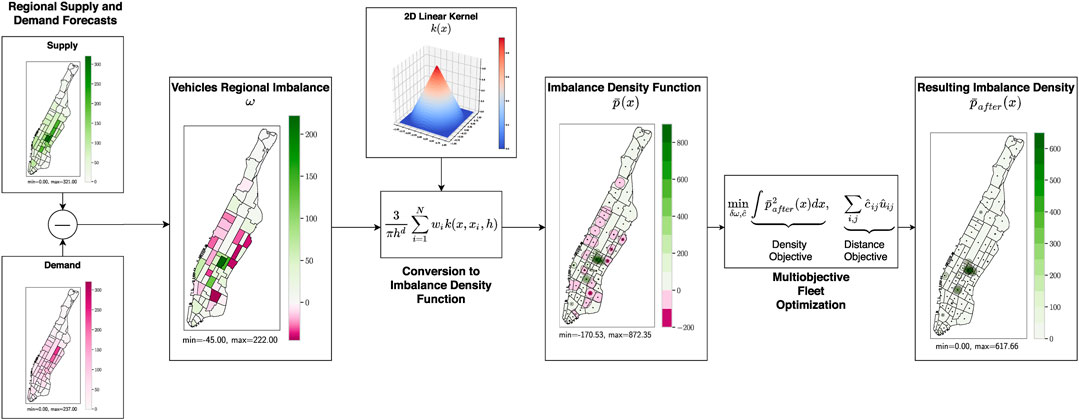
FIGURE 3. The flow of the reachability function-based repositioning (RFR) strategy with vehicle supply and demand aggregated over zone centroids.
We first introduce a general version that purely aims at minimizing the supply-demand imbalance density and the repositioning distance objectives without any restriction on zones—contrary to the traditional restriction of sending vehicles only from surplus to deficiency regions. Because of the ability to send vehicle to or from any region, we will refer to the formulation in the current section as RFR with regions and full flow (RFRRf). The next section will introduce a formulation with constraints on origin and destination regions.
Consider a region-based repositioning problem as defined in Section 2.5. Let
where
For calculating the difference between supply and demand densities in Eq. 9i, we use the integral of squared deviation as it puts more importance on high imbalance values than other metrics, e.g., the integral of absolute deviation. Additionally, it significantly reduces the computational effort as described below:
With the definition of matrix
The constant term
where
Furthermore, another advantage of the formulation is that it is not even necessary to use the same bandwidth h for all zones or the complete day. According to the statistics of the zone, the bandwidth or reachability can be chosen differently. For example, for the outskirts of a city or low traffic zones, we can choose a larger bandwidth as the vehicle can pick up a customer from larger distances. Conversely, for the zones with lower traffic speeds (near the city center), we can choose smaller bandwidths.
It should also be noted that as h approaches zero (no overlap of the kernel functions),
In this form, the measurement of the imbalance of a region is independent of the imbalances in other regions. However, it is still quite different from the traditional repositioning formulation that applies the balancing of regions as constraints of the optimization problem and minimizes the repositioning VKT (Pavone et al., 2012; Alonso-Mora et al., 2017a). Because of the multi-objective formulation in Eq. 9 and the square of zone weights in Eq. 14, the obtained repositioning problem will give a higher preference to balancing the regions with higher imbalances—allowing the vehicles to be sent to far off regions as well, in contrast to traditional repositioning that limits it to the closest regions as described in Section 1.1.
Since the vehicle supply and demand densities are more general than the regional surplus and deficiency, the flow of vehicles in the RFRRf formulation was kept general—to and from all regions irrespective of local imbalances—to allow the minimization of overall density. However, since we use integral squared deviation to reduce the computational effort for the density objective (Eq. 12), even small differences in the density objective could be overemphasized during the optimization process. Secondly, the regional demands vary significantly during night and day hours; during the early morning hours with little to no demand, the RFRRf formulation would try to distribute all vehicles evenly throughout the city to decrease the imbalance density. This could lead to increased repositioning of vehicles without a significant increase in the overall performance. Thus, this section presents formulations that restrict the flow of vehicles from certain regions based on local imbalance to lower the above effects. We put these restrictions in two steps:
1. Since the RFRRf formulation is general, it even allows for the repositioning of vehicles from deficiency zones to other zones. This will lower the short-term density, but may make even available vehicles in the deficient zones busy with repositioning; ultimately, leading to decreased performance gain. Thus, we limit this effect by changing the constraint in Eq. 9e with the following:
The above constraints restrict the negative changes in a zone (the outflow of vehicles) at zero if the original zone weight is negative (i.e., deficient zone). Since this formulation only allows for the outflow of vehicles from surplus (zones with positive weights), we refer to this formulation as RFRRp.
2. As final step to zone-based restrictions, we only allow the repositioning of vehicles from surplus to deficiency zones. We refer to this formulation simply by RFRR. The previously described RFRRp allowed the repositioning from surplus zones to all zones which could still cause excessive repositioning VKT. Even though bringing a higher number of vehicles to a zone can benefit if demand and supply forecasts contain uncertainties, it can cause unnecessary repositioning especially when most zones are not balanced. Therefore, the following RFRR approach can limit unnecessary repositioning further while simultaneously simplifying the formulation the number of variables and the required matrix sizes are decreased.
Notice the decrease in the size of flow variables matrix
The presented repositioning approach in Eq. 9 is a multi-objective optimization problem. We first present the approach where we give the highest preference to the density objective. In the subsequent section we formulate the problem for finding the pareto fronts.
If the priority of objectives is known beforehand in a multi-objective optimization problem, the lexicographic method is generally used (Chang, 2015). One major advantage of the method is that it gives a pareto optimal solution without the need of scaling the individual objectives. In a lexicographic method, the problem is solved separately, first for the highest priority objective. Then, the already solved objectives with the optimal values are put as constraints while solving the problem for the next objective. Since we use separate variables
The weighted sum method is a well known multi-objective method, where individual objectives are multiplied by constant weights for relative importance. The assigned weights help to move over pareto front solutions. However, as the units and the magnitude of the individual objectives may vary for different problem instances, it requires a meaningful scaling of the individual objectives. In the current study, we use the well-known approach of scaling the objectives using nadir and utopian values (Grodzevich and Romanko, 2006). Thus, the multi-objective function in Eq. 16a can be written as:
where
The utopian and nadir points are obtained from the pareto optimal set of solutions. This set is usually obtained by optimizing the individual objectives with the original constraints. The lower bounds of the individual objectives form the utopian point and the upper bounds form the nadir point.
In the current problem formulation, it is sufficient to consider two extreme pareto solutions for finding the utopian and nadir points. The distance objective
Generally, because of the dynamic nature of RH services, the benefits of a repositioning decision cannot be evaluated until the realization of the actual customer demand in the system. For a repositioning algorithm, it is usually difficult to evaluate the long-term impacts of a decision. Therefore, the goal is to empirically show the correlations between various KPIs and long-term repositioning performance. Following the same zone definitions as in Section 2.5, we introduce the following KPIs:
where
In this study, the correlation of these KPIs, which can be evaluated instantaneously (before and after the decision to reposition), and long-term fleet performance are analyzed. In general, repositioning only generates costs for sending the vehicle to another place in the operating area at the time of the decision. Assigning instantaneous rewards, which estimate the benefits over the course of time, can be very useful for approximate dynamic programming approaches like reinforcement learning.
Before applying the suggested methods in a dynamic simulation, it is useful to understand the basic principles and differences of the various suggested approaches on concrete static instances. This is also very important for analyzing the aggregated long-term simulation outcomes. Therefore, the current section presents numerical experiments on static instances.
We use the open source NYC taxi data to generate the static repositioning scenario from November 13, 2018. The data are geographically aggregated into NYC taxi zones for privacy reasons. The definition and shape of these zones are already provided and for consistency we use the same zones for repositioning. We only considered the trips originating and ending in the Manhattan area of the city, which constitutes 63 taxi zones.
Since the geographical distribution of customer origins and destinations varies significantly between morning and evening, we generate test cases by accumulating the customer requests from two time periods: from 9 to 9:15 am and from 6 to 6:15 pm. For the two periods, we generate idle cars by taking the destination zones of randomly picked customer requests from the 1 h period before 9 am and 6 pm, respectively. According to the trip data, we have a total of 3,265 and 4,409 customers for 9 am and 6 pm, respectively.
In this section, we keep the bandwidth h as 1.5 km, which equals a maximum allowed pick-up delay of
We first experiment with increasing values of γ. As shown in Figure 4, the repositioning problem has conflicting objectives which is apparent from the pareto front in distance vs. density plots. With varying values of γ, the solution values build the pareto front. As described in Section 3.5.2, the PBD solutions form the end points of the pareto front for each method. It can be observed that the region-focused min-distance method is not on the pareto fronts of either method and RFRRf provides the best compromise between the two objectives. Thus, VRF-based methods provide a better compromise of the vehicle balance density and distance objectives.
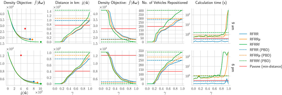
FIGURE 4. The impacts of increasing γ on the suggested RFRR methods for the static problem instances taken from morning (9 a.m.) and evening (6 p.m.). The instances use 500 idle vehicles and RFRR bandwidths (h) of 1.5 km. The calculation time does not include the time required for the PBD step, which is provided separately in the plots.
Figure 4 also shows that with
Figure 4 also shows that as more zone restrictions are put in the RFRRf formulation via RFRRp and RFRR, the density objective becomes worse. However, RFRRf (and RFRRp to a lesser degree) achieves slightly better density objectives by compromising a significant number of repositioning vehicles and VKT. This is apparent from the pareto front in Figure 4, where the difference of
For the 9 am scenario, we see that all VRF-based approaches produce better density objectives than the min-distance method. The same PBD solutions of Figure 4 are visualized on the map in Figure 5. It can be seen that the min-distance strategy treated the regions individually and tried to distribute the excess vehicles equally among regions while minimizing the VKT. This left the zones in the upper east and west side regions highly deficient. In comparison, VRF-based methods focus on the overall distribution, and thus, send more vehicles to the upper east and west sides. Notice that since the RFRRf can send vehicles from and to all possible combinations of regions to decrease the density objective, the RFRRf minimum region deficiency weight in Figure 5 is even less than the original zone imbalance weights. The reason is that the RFRRf method even repositioned some idle vehicles from the deficiency regions to minimize the imbalance density.
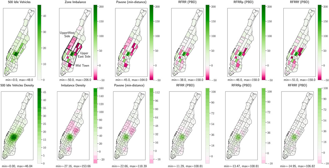
FIGURE 5. Results of various repositioning methods for a 9 am static case. The first row shows the zone counts for the idle vehicles and the imbalances while the second row shows the heat-map of densities calculated using Eq. 8 with
In the dynamic simulation, the number of available idle vehicles keeps changing according to customer demands. Therefore, Figure 6 shows the experiment with a growing number of idle vehicles. We generate new vehicles using the same procedure as described in the previous section and incrementally add them to the idle vehicle weights. The most important observations are:
• Looking at the density objective, we observe that for all the VRF methods there is a critical number of vehicles at which the density objective is the least, and the possible benefit from the applied repositioning method is maximum. We will refer to this point as vehicle saturation point (VSP).
• We also observe that the VRF-based methods can change the absolute value of imbalance density
• For fleet sizes larger than the VSP, the density objective increases as the additional vehicles contribute more toward increasing the surplus then being used to fulfill the vehicle deficiency, which is evident by comparing the values of total surplus
• Compared to the min-distance method, the VRF-based methods perform much better for balancing the deficiency value
• Since we use integral square deviation for the density objective in Eq. 9i, all the VRF-based methods are equally sensitive for both surplus and deficiency, not just for deficiency. Therefore, we observe that RFRRp and RFRRf keep repositioning more vehicles to balance the surplus density for the added vehicles even when
• The RFRR method provides the best compromise among all methods. With a lower number of idle vehicles, it repositions enough vehicles—more than the min-distance method and similar in amount to RFRRf and RFRRp—to reduce vehicle deficiency, i.e.,
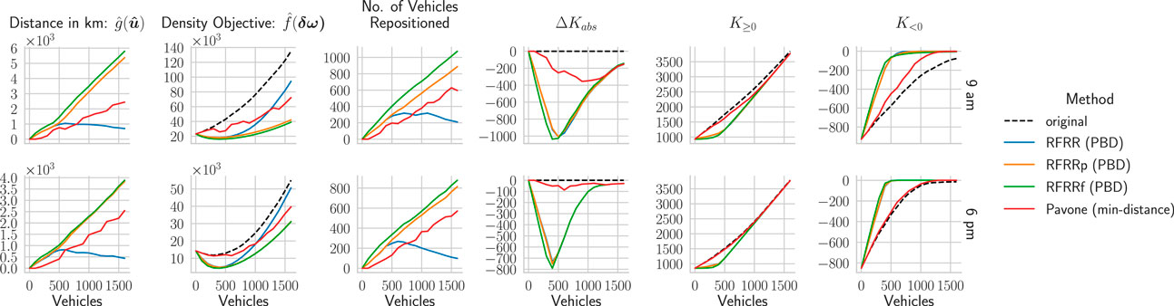
FIGURE 6. The impacts of increasing the number of idle vehicles on the suggested RFRR methods for the static problem instances taken from morning (9 a.m.) and evening (6 p.m.). The values of the original position correspond to the values without any repositioning. Additionally,
We use an agent-based simulation environment for our experiments. The environment consists of three types of agents: operator, customers, and vehicles controlled by the operator. Each scenario with particular parameter setting is simulated for one week of data. For the first day of the simulation, the same initial vehicle positions are used for all the scenarios. However, considering that the simulation takes some time to warm up and distribute the vehicles more naturally than the initial distribution, the simulations include a warm-up period of 1 h.
In each simulation step, the time t is incremented by 1 s and the system state is updated accordingly. For the vehicle-customer assignment, the system state consists of vehicles’ current locations, the newly generated customers, and the information regarding currently serving, fulfilled, or expired customer requests. The new requests are batched every 30 s after which the batch assignment problem is solved. Similarly, after every
For solving the optimization problems, we use the commercial MIP solver CPLEX with its Python API. The rest of the data processing and simulation is written in Python 3.7.
We use the same NYC taxi data from November 12, 2018 to November 18, 2018. As described in Section 4.1, the data do not provide the exact start and end location of a trip, rather the trips are aggregated over areas of different sizes called NYC taxi zones. The trip data and the definition and shape of these zones are provided by the authorities and for consistency we use the same zones for repositioning. We only considered the trips originating and ending in the Manhattan borough. Furthermore, we filtered probable false trip records in the data with speeds below 1 m/s or above 30 m/s.
We extract the drivable street network from OpenStreetMap data using the Python library called OSMnx (Boeing, 2017). For reducing the computational efforts, we first simplify the network using the built in OSMnx simplification procedure that keeps only the intersection and end-point nodes. We define all nodes as boarding nodes that are only connected to roads of the classes “living street”, “residential”, “primary”, “secondary”, and “tertiary”. The NYC taxi data are disaggregated by assigning the pick-up and drop-off locations of the aggregated customers data to boarding nodes in the respective zones randomly.
We assign link travel times using the free-flow speeds already provided for the links. If any link does not have speed information we set it as 25 mph (approximately 40 km/h). In order to replicate realistic travel times, the speeds of all links were scaled after every 15 min according to the average speeds by comparing the free-flow and recorded travel times of the actual trips from the NYC taxi data in the last 15 min (see Section 1 of Supplementary Material for details of the scaling procedure). Additionally, we use a maximum customer waiting time
Following a similar experimental approach to the static results section, we first concentrate on the long-term impacts of the presented repositioning approaches with varying values of γ and the total fleet size while keeping a fixed kernel bandwidth h of 1.5 km. We also fix the profit parameters in Eq. 1, i.e.,
Figure 7 shows the overall results of the simulated week. As shown in Figure 7A, the repositioning distance, served customers, and the overall profit increases with γ. The performances of all the presented kernel-based methods surpass that of the traditional min-distance strategy for higher values of γ. Additionally, the value of γ gives a good benchmark on how much an MSP is willing to reposition vehicles for long-term profit gains.
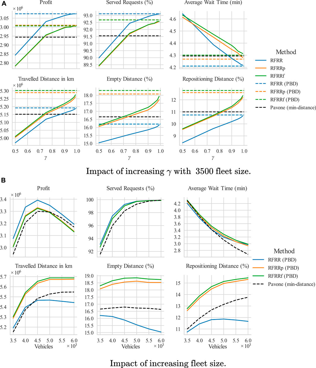
FIGURE 7. Results of one week of simulation on NYC data from November 12–18, 2018. The empty distance consists of both customer pick-up and the repositioning distances. In (A) the plots only include evaluations until
In the studied framework, en-route repositioning vehicles cannot be re-assigned by myopic customer-vehicle batch optimizations (unaware of demand and supply forecasts) before coming close to the destination. Therefore, increasing vehicle balance through repositioning has two trade-offs: 1) these vehicles are not available for customer assignment thereby reducing the effective fleet size; 2) the repositioning trips are empty thereby generating costs without immediate revenue. Only if these trips generate additional revenue by serving more customers, can more profit can be achieved. Therefore, we notice that in Figure 7A the extra repositioning distances in RFRRp and RFRRf kept vehicles more busy than RFRR for all values of γ, leading to fewer served customers and less profit than the RFRR approach.
Figure 7B compares the performance with varying fleet size. The first observation is the profit term. For all the repositioning methods, increasing the fleet sizes increases the overall profit as the operator can serve more customers. However, after the saturation points (i.e., 4,500 vehicles), increasing the fleet size decreases the profit because of the increase in the maintenance costs with fleet size without more customers to serve. We also observe that the presented kernel-based approaches outperform the min-distance strategy for all fleet sizes. RFRR (PBD) performs the best among them indicating a higher priority to eradicate vehicle deficits than to balance vehicle surplus over the operating area.
Interestingly, even though the major aim of the min-distance method is to reduce the repositioning VKT, the focus on strictly distributing the excess vehicles equally among regions and reducing immediate repositioning VKT ultimately leads to more repositioning VKT in the long-term. There are a few reasons contributing to this result. First, the density-based algorithms aim to minimize the overall imbalance in the whole operating area instead of individual zones, which can produce better vehicle distributions and therefore less repositioning for the subsequent repositioning problem instances. Moreover, some short repositioning trips between small neighboring zones might not improve the overall balance of demand and supply and are not recommended by the density-based algorithms. Additionally, it might be sufficient to choose a destination that is closer to the idle vehicles than a small-sized deficit zone as vehicles from the nearby zone can cover that area as well. Furthermore, as observed in Section 4.2, the min-distance strategy repositions unnecessarily more vehicles with an increasing number of idle vehicle to balance excess vehicles equally. This would be especially problematic at off-peak times when there is a higher number of idle vehicles. In light of the above observation, the superior performance of the RFRR method (PBD) in Figure 7B is clearly understandable, where the repositioning distances are less and served customers are more than the min-distance method. The better customer coverage inherent in the RFRR method leads to overall decreased repositioning distances in the long-term.
Lastly, we evaluate the impacts of increasing repositioning on the profit components. Figure 8 evaluates the performance of the whole week for increasing value of base price (ζ), unserved penalty (ξ), and γ while keeping distance-based fare (
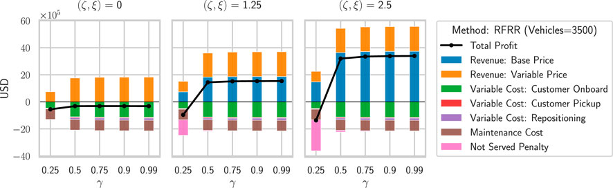
FIGURE 8. Impact of increasing the relative importance of density objective (γ), base customer fare (ζ), and the future adjustment cost for not serving a customer (ξ).
Using the simulation of the week, we study the correlation of KPIs in Section 3.6 with the long-term effect of repositioning decisions. Every time a repositioning algorithm is called, we calculate the KPIs using the zone weights returned from the repositioning solution. Then we look at the correlation of calculated KPIs with the actual number of served or unserved customers within different time periods after the repositioning step; the different time periods can have different correlations, since it takes some time for vehicles to reach their destinations.
Figure 9 shows the correlations of KPIs with the customer statistics. Since we simulated multiple fleet sizes, we also observe correlations by scaling the customer stats by fleet sizes. As shown in Figure 9B,
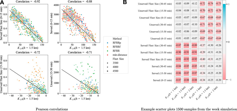
FIGURE 9. Correlation of instantaneous integral KPIs with long-term customer service quality.
The comparison of
Lastly, we study the relation of kernel bandwidths (h) and the maximum allowed customer pick-up time (
Figure 10 presents results for a fleet size of 4,500 vehicles. It indeed illustrates that for a very short waiting time of 2 min, a kernel bandwidth h of 2 km serves approximately 3–4% fewer customers. For larger maximum waiting times, the number of served customers converges for different bandwidths. Simulations with smaller fleet sizes (unsaturated demand) showed the same behavior.
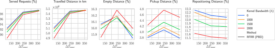
FIGURE 10. The impact of changing the maximum allowed waiting time
For accurate forecasts, the bandwidth parameter generates a trade-off between empty repositioning and pick-up distances. For larger bandwidths, vehicle repositioning considers the area that a vehicle can cover for a pick-up trip—defined as the empty VKT a vehicle has to make to pick up an assigned customer request. For a larger h, the pick-up VKT will be increased as the vehicles will have to cover a larger area. Figure 10 shows that the sum of pick-up and repositioning in our simulations is nearly constant for different bandwidth values, which is a sign that the forecast accuracy is really high; in this case study, future trip data within the future horizon of 30 min were aggregated thereby producing a forecast with perfect accuracy for the given spatial and temporal precision. As the forecasts typically show stochastic errors, prioritizing pick-up distance over repositioning distance should typically produce lower shares of empty miles in practice.
In conclusion, we presented a kernel or reachability function-based repositioning approach for RH services. Using 2D kernel functions, we introduced the concept of a 2D imbalance density, which consistently describes the imbalances of the overall operation area irrespective of the definition of individual zones. The density function naturally takes into account the proximity and inter-region distances. This method was utilized to introduce an innovative repositioning formulation that removed a fundamental problem in earlier repositioning approaches; they considered each zone individually whereas our approach considers the proximity of other regions.
With the 2D density function, we presented three repositioning formulations: RFRR, RFRRp, and RFRRf, which showed a significant improvement over the state of the art strategies. Among all the methods, RFRR performed the best from which we concluded that even though the presented formulations take into account the overall operation area in the form of density, the performance is further increased by restricting the flow of vehicles from surplus to deficiency regions only.
We also introduced kernel-based KPIs and showed their correlations with long-term fleet performance.
The service models and operational forms of MOD services are vast. The study design clearly demarcates the assumed MOD mode (AV-based RH service without pooling), the associated profit objective, and the experimented NYC taxi dataset. For simplicity, we derived the future customer regional statistics directly from the data; in real RH applications, such perfect knowledge of future customers may not be available. The performance of the presented strategy should be evaluated with realistic, erroneous forecasts using techniques like machine learning (Ke et al., 2017). Additionally, the assignment of a vehicle to a customer in the studied scenario is a highly dynamic problem. We used a specific strategy with a specific objective function for assignment. A different assignment strategy can also change the results. Similarly, we used simplistic scaling of travel times using the ratio of total travel duration. While such scaling is more realistic than free-flow speeds, it does not represent reality. It is possible that a simulated vehicle is able to pick up a customer on time, but in reality, it is not able to do that. Thus, the simulated performance for specific fleet size can differ from the actual Manhattan data. Lastly, there is also no guarantee that the approach will behave similarly in other cities with a much larger operating area, as the Manhattan area is small compared to other cities, in which RH services are operated.
With the above limitations, the presented work is a significant scientific step toward improved repositioning and a better fleet utilization. Future research should focus on using the presented approach in different operation areas with more realistic travel times, datasets, and vehicle assignment objectives to confirm the usefulness of the presented strategy.
In the current work, we also limited the kernel bandwidths to fixed lengths, while in reality, the reachable distance of vehicles differs significantly throughout the day. Future works should focus on using an adaptive kernel bandwidth according to the current network speed. In theory, the method could even work with different speeds and thereby differing reachability bandwidths for the areas in the network. Similarly, we used a specific forecast period (30 min) and definition of zone imbalances for measuring the 2D imbalance density. We expect that studying different forecast periods and zone weights can improve the performance further. It might also be interesting to consider available parking spots (as in Winter et al., 2020) and define the reachability around likely parking locations to find suitable destinations of repositioning vehicles.
Finally, the density model can be applied whenever stochastic spatio-temporal information is used. This could help to further improve other recent developments like multiple repositioning time horizons (e.g., Albert et al., 2019; Dandl et al., 2020) or combined assignment and repositioning with dynamic programming (e.g., Al-Kanj et al., 2020). Moreover, with the presented definition of the 2D imbalance density and the long-term performance KPIs, we expect that modern machine learning algorithms can benefit significantly. These algorithms have proven performance for learning relations among multitudes of variables. Since an effective fleet control and repositioning strategy will have to consider multiple short-term and long-term performance indicators, we expect that a statistical technique can significantly improve the overall performance.
Publicly available datasets were analyzed in this study. This data can be found here: New York City Yellow Taxi data. The used data is from 12th to 18th November, 2018. https://www1.nyc.gov/site/tlc/about/tlc-trip-record-data.page.
AAS: Conceptualization, methodology, software, formal analysis, writing—original draft, writing—review and editing, and visualization. FD: Conceptualization, methodology, software, formal analysis, writing—original draft, and writing—review and editing. BK: Conceptualization, writing—review and editing, and supervision. KB: Conceptualization, writing—review and editing, and supervision.
The authors declare that the research was conducted in the absence of any commercial or financial relationships that could be construed as a potential conflict of interest.
The Supplementary Material for this article can be found online at: https://www.frontiersin.org/articles/10.3389/ffutr.2021.681451/full#supplementary-material
Agatz, N., Erera, A., Savelsbergh, M., and Wang, X. (2012). Optimization for Dynamic Ride-Sharing: A Review. Eur. J. Oper. Res. 223, 295–303. doi:10.1016/j.ejor.2012.05.028
Al-Kanj, L., Nascimento, J., and Powell, W. B. (2020). Approximate Dynamic Programming for Planning a Ride-Hailing System Using Autonomous Fleets of Electric Vehicles. Eur. J. Oper. Res. 284, 1088–1106. doi:10.1016/j.ejor.2020.01.033
Albert, M., Ruch, C., and Frazzoli, E. (2019). Imbalance in Mobility-On-Demand Systems. ACM Trans. Spat. Algorithms Syst. 5, 1–22. doi:10.1145/3325914
Alonso-Mora, J., Samaranayake, S., Wallar, A., Frazzoli, E., and Rus, D. (2017a). On-demand High-Capacity Ride-Sharing via Dynamic Trip-Vehicle Assignment. Proc. Natl. Acad. Sci. USA 114, 462–467. doi:10.1073/pnas.1611675114
Alonso-Mora, J., Wallar, A., and Rus, D. (2017b). “Predictive Routing for Autonomous Mobility-On-Demand Systems with Ride-Sharing,” in 2017 IEEE/RSJ International Conference on Intelligent Robots and Systems (IROS) September 24–28, 2017 Vancouver, BC, Canada:(IEEE), 3583–3590.
Boeing, G. (2017). Osmnx: New Methods for Acquiring, Constructing, Analyzing, and Visualizing Complex Street Networks. Comput. Environ. Urban Syst. 65, 126–139. doi:10.1016/j.compenvurbsys.2017.05.004
Chang, K.-H. (2015). “Multiobjective Optimization and Advanced Topics,” in e-Design Boston:Academic Press, Elsevier, 1105–1173. doi:10.1016/B978-0-12-382038-9.00019-3
Chen, Y.-C. (2017). A Tutorial on Kernel Density Estimation and Recent Advances. Biostatistics Epidemiol. 1, 161–187. doi:10.1080/24709360.2017.1396742
Dandl, F., and Bogenberger, K. (2019). Comparing Future Autonomous Electric Taxis with an Existing Free-Floating Carsharing System. IEEE Trans. Intell. Transport. Syst. 20, 2037–2047. doi:10.1109/TITS.2018.2857208
Dandl, F., Engelhardt, R., Hyland, M., Tilg, G., Bogenberger, K., and Mahmassani, H. S. (2021). Regulating Mobility-On-Demand Services: Tri-level Model and Bayesian Optimization Solution Approach. Transportation Res. C: Emerging Tech. 125, 103075. doi:10.1016/j.trc.2021.103075
Dandl, F., Hyland, M., Bogenberger, K., and Mahmassani, H. S. (2020). “Dual-horizon Forecasts and Repositioning Strategies for Operating Shared Autonomous Mobility Fleets,” in Annual Meeting of the Transportation Research Board January 12–16, 2020 Washington, DC.
Dandl, F., Hyland, M., Bogenberger, K., and Mahmassani, H. S. (2019). Evaluating the Impact of Spatio-Temporal Demand Forecast Aggregation on the Operational Performance of Shared Autonomous Mobility Fleets. Transportation 46, 1975–1996. doi:10.1007/s11116-019-10007-9
Engelhardt, R., Dandl, F., Bilali, A., and Bogenberger, K. (2019). “Quantifying the Benefits of Autonomous On-Demand Ride-Pooling: A Simulation Study for munich, germany,” in 2019 IEEE Intelligent Transportation Systems Conference (ITSC) October 27–30, 2019 Auckland, New Zealand:(IEEE), 2992–2997.
Erdmann, M., Dandl, F., and Bogenberger, K. (2019). “Dynamic Car-Passenger Matching Based on Tabu Search Using Global Optimization with Time Windows,” in 2019 8th International Conference on Modeling Simulation and Applied Optimization (ICMSAO) April 15–17, 2019 Manama, Bahrain:(IEEE), 1–5.
Fagnant, D. J., Kockelman, K. M., and Bansal, P. (2015). Operations of Shared Autonomous Vehicle Fleet for austin, texas, Market. Transportation Res. Rec. 2563, 98–106. doi:10.3141/2536-12
Fagnant, D. J., and Kockelman, K. M. (2014). The Travel and Environmental Implications of Shared Autonomous Vehicles, Using Agent-Based Model Scenarios. Transportation Res. Part C: Emerging Tech. 40, 1–13. doi:10.1016/j.trc.2013.12.001
Grodzevich, O., and Romanko, O. (2006). Normalization and Other Topics in Multi-Objective Optimization Toronto, Canada: The Fields Institute for Research in Mathematical Sciences (FIELDS).
Hamzehi, S., Bogenberger, K., Franeck, P., and Kaltenhäuser, B. (2019). “Combinatorial Reinforcement Learning of Linear Assignment Problems,” in 2019 IEEE Intelligent Transportation Systems Conference (ITSC) (IEEE), 3314–3321.
Henao, A., and Marshall, W. E. (2019). The Impact of Ride-Hailing on Vehicle miles Traveled. Transportation 46, 2173–2194. doi:10.1007/s11116-018-9923-2
Ho, S. C., Szeto, W. Y., Kuo, Y.-H., Leung, J. M. Y., Petering, M., and Tou, T. W. H. (2018). A Survey of Dial-A-Ride Problems: Literature Review and Recent Developments. Transportation Res. B: Methodological 111, 395–421. doi:10.1016/j.trb.2018.02.001
Hottung, A., and Tierney, K. (2019). “Neural Large Neighborhood Search for the Capacitated Vehicle Routing Problem,” in Proc. 24th Eur. Conf. Artif. Intell. - ECAI 2020 29 August – 8 September, 2020.
Hyland, M., Dandl, F., Bogenberger, K., and Mahmassani, H. (2019). Integrating Demand Forecasts into the Operational Strategies of Shared Automated Vehicle Mobility Services: Spatial Resolution Impacts. Transportation Lett. 12, 671–676. doi:10.1080/19427867.2019.1691297
Hyland, M., and Mahmassani, H. S. (2018). Dynamic Autonomous Vehicle Fleet Operations: Optimization-Based Strategies to Assign Avs to Immediate Traveler Demand Requests. Transportation Res. Part C: Emerging Tech. 92, 278–297. doi:10.1016/j.trc.2018.05.003
Hyland, M., and Mahmassani, H. S. (2020). Operational Benefits and Challenges of Shared-Ride Automated Mobility-On-Demand Services. Transportation Res. A: Pol. Pract. 134, 251–270. doi:10.1016/j.tra.2020.02.017
Kaltenhäuser, B., Werdich, K., Dandl, F., and Bogenberger, K. (2020). Market Development of Autonomous Driving in germany. Transportation Res. Part A: Pol. Pract. 132, 882–910. doi:10.1016/j.tra.2020.01.001
Ke, J., Zheng, H., Yang, H., and Chen, X. (2017). Short-term Forecasting of Passenger Demand under On-Demand Ride Services: A Spatio-Temporal Deep Learning Approach. Transportation Res. Part C: Emerging Tech. 85, 591–608. doi:10.1016/j.trc.2017.10.016
Maciejewski, M., Bischoff, J., and Nagel, K. (2016). An Assignment-Based Approach to Efficient Real-Time City-Scale Taxi Dispatching. IEEE Intell. Syst. 31, 68–77. doi:10.1109/mis.2016.2
Mao, C., Liu, Y., and Shen, Z.-J. (2020). Dispatch of Autonomous Vehicles for Taxi Services: A Deep Reinforcement Learning Approach. Transportation Res. Part C: Emerging Tech. 115, 102626. doi:10.1016/j.trc.2020.102626
Nazari, M., Oroojlooy, A., Snyder, L., and Takác, M. (2018). “Reinforcement Learning for Solving the Vehicle Routing Problem,” in Advances in Neural Information Processing Systems December 3, 2018Curran Associates Inc, 9839–9849.
Parzen, E. (1962). On Estimation of a Probability Density Function and Mode. Ann. Math. Statist. 33, 1065–1076. doi:10.1214/aoms/1177704472
Pavone, M., Smith, S. L., Frazzoli, E., and Rus, D. (2012). Robotic Load Balancing for Mobility-On-Demand Systems. Int. J. Robotics Res. 31, 839–854. doi:10.1177/0278364912444766
Pouls, M., Meyer, A., and Ahuja, N. (2020). “Idle Vehicle Repositioning for Dynamic Ride-Sharing,” in Computational Logistics. Vol. 12433 of Lecture Notes in Computer Science. Editors E. Lalla-Ruiz, M. Mes, and S. Voß (Cham: Springer International Publishing), 507–521. doi:10.1007/978-3-030-59747-4_33
Sayarshad, H. R., and Chow, J. Y. J. (2017). Non-myopic Relocation of Idle Mobility-On-Demand Vehicles as a Dynamic Location-Allocation-Queueing Problem. Transportation Res. E: Logistics Transportation Rev. 106, 60–77. doi:10.1016/j.tre.2017.08.003
Syed, A. A., Akhnoukh, K., Kaltenhaeuser, B., and Bogenberger, K. (2019a). “Neural Network Based Large Neighborhood Search Algorithm for Ride Hailing Services,” in EPIA Conference on Artificial Intelligence September 3–6, 2019 Vila Real, Portugal:Springer, 584–595. doi:10.1007/978-3-030-30241-2_49
Syed, A. A., Kaltenhaeuser, B., Gaponova, I., and Bogenberger, K. (2019b). “Asynchronous Adaptive Large Neighborhood Search Algorithm for Dynamic Matching Problem in Ride Hailing Services,” in 2019 IEEE Intelligent Transportation Systems Conference (ITSC) October 27–30, 2019 Auckland, New Zealand:IEEE, 3006–3012.
Toth, P., and Vigo, D. (2014). Vehicle Routing: Problems, Methods, and Applications Philadelphia: Society for Industrial and Applied Mathematics (SIAM) Publications.
Wallar, A., Van Der Zee, M., Alonso-Mora, J., and Rus, D. (2018). “Vehicle Rebalancing for Mobility-On-Demand Systems with Ride-Sharing,” in 2018 IEEE/RSJ International Conference on Intelligent Robots and Systems (IROS) October 1–5, 2018 Madrid, Spain:IEEE, 4539–4546.
Weikl, S., and Bogenberger, K. (2015). A Practice-Ready Relocation Model for Free-Floating Carsharing Systems with Electric Vehicles - Mesoscopic Approach and Field Trial Results. Transportation Res. Part C: Emerging Tech. 57, 206–223. doi:10.1016/j.trc.2015.06.024
Weikl, S., and Bogenberger, K. (2013). Relocation Strategies and Algorithms for Free-Floating Car Sharing Systems. IEEE Intell. Transport. Syst. Mag. 5, 100–111. doi:10.1109/mits.2013.2267810
Keywords: repositioning, correlation, vehicle imbalance, vehicle distribution, ride sharing, ride hailing, kernel density estimation, mobility on demand
Citation: Syed AA, Dandl F, Kaltenhäuser B and Bogenberger K (2021) Density Based Distribution Model for Repositioning Strategies of Ride Hailing Services. Front. Future Transp. 2:681451. doi: 10.3389/ffutr.2021.681451
Received: 16 March 2021; Accepted: 03 May 2021;
Published: 14 June 2021.
Edited by:
Francesco Viti, University of Luxembourg, LuxembourgReviewed by:
Tai-Yu Ma, Luxembourg Institute of Socio-Economic Research, LuxembourgCopyright © 2021 Syed, Dandl, Kaltenhäuser and Bogenberger. This is an open-access article distributed under the terms of the Creative Commons Attribution License (CC BY). The use, distribution or reproduction in other forums is permitted, provided the original author(s) and the copyright owner(s) are credited and that the original publication in this journal is cited, in accordance with accepted academic practice. No use, distribution or reproduction is permitted which does not comply with these terms.
*Correspondence: Arslan Ali Syed, YXJzbGFuLnN5ZWRAdHVtLmRl
Disclaimer: All claims expressed in this article are solely those of the authors and do not necessarily represent those of their affiliated organizations, or those of the publisher, the editors and the reviewers. Any product that may be evaluated in this article or claim that may be made by its manufacturer is not guaranteed or endorsed by the publisher.
Research integrity at Frontiers
Learn more about the work of our research integrity team to safeguard the quality of each article we publish.