Empowering Compartmental Modeling With Mobility and Shelter-in-Place Analysis

A model that is capable of handling the non-linear trend of COVID-19 throughout the US and evaluate different effects of interstate/intrastate mobility measures can help decision-makers adjust guidelines and state-wide mandates to contain the pandemic's spread. The abundance of cellular-based data has made it possible to study many aspects of users' mobility, including their travel, contact, and dwell patterns. This study uses a compartmental metapopulation model to present a correlation between the contact and mobility indices and the likelihood of being susceptible to infection. We studied the effect of travel from other states on overall infections in a destination state and observed a strong inverse correlation of 0.98 between the contact index and social awareness compartment, i.e., individuals who are no longer susceptible to infection. The shelter-in-place what-if analysis for travelers from other states on the course of infection in the destination state showed a possible reduction of over 22% in the total number of infections and death if travelers sheltered in place for 5–7 days.

1. Introduction

In December 2019, a viral infection caused by the SARS-CoV-2 virus took the world by surprise. In a span of 2 months, this virus had spread to over 20 countries worldwide (Dong et al., 2020). It was classified as the COVID-19 pandemic by the World Health Organization on February 11, 2020. Based on the Centers for Disease Control and Prevention (CDC), the first case of the novel coronavirus was introduced to the US on January 15, 2020, through travel from Wuhan, China (CDC, 2020). On January 17, 2020, CDC implemented health screening measures for travelers at several major US airports. This signifies that the effect of travel in the spreading of the novel coronavirus outbreak cannot be ignored (Wells et al., 2020).

For over a century, compartmentalized epidemiological models, generally referred to as the susceptible, exposed, infected, recovered, and dead (SEIRD) models, have been considered the best tool for modeling the trend of epidemics. These models share an ordinary differential equation (ODE) at their core; however, most epidemiological models are based on the presumption of a constant population divided into compartments and model individuals' transition from one compartment to another but do not consider travel from one location to another.

COVID-19 has occurred at a time where detailed mobility data is abundant and readily available. For example, analysis of cellular signals has made it possible to determine several mobility measures (such as mobility index, contact index, and at-home) (Cuebiq, 2020a,c), which can be used to study the effect of travels and enhance the epidemiological modeling.

This study aims to present a hybrid modeling methodology using the model presented in Bakhtiari Ramezani et al. (2021) and study the correlation of social awareness with interstate/intrastate mobility and contact indices in the US. This study also aims at determining the effect of traveling by exposed travelers to a destination state, who do not adhere to shelter-in-place guidelines, on overall exposures and infections. Section 2 provides an overview of the compartmental models and basic assumptions surrounding them. Section 3 discusses methodology and data gathering approaches used in the present work. Section 4 examines correlations between observed mobility data and modeling outcomes for the state of Alabama.

2. Background

Basic epidemiological modeling of the disease through ODEs is a challenging task for the recent pandemic due to the lack of an accurate model that can handle the non-linear behavior being observed (e.g., Chatterjee et al., 2020; Fernández-Villaverde and Jones, 2020; Jia et al., 2020; Lingzhi et al., 2020; Moghadas et al., 2020; Volpatto et al., 2020; Wang et al., 2020). What makes it even more challenging to model the COVID-19 pandemic trend is the introduction of social distancing measures, states of emergency, and stay-at-home orders.

Belik et al. (2011) have presented a model to account for movements to and from destinations based on mobility networks. They used meta-population network topology and calculated the epidemic's velocity, highlighting the importance of considering mobility in spatial epidemic models. Similarly, Pei et al. (2018) used a meta-population model to study the Spatio-temporal spreading of influenza and incorporated the mobility data into their model. Their human-centered model could predict the onset of the outbreak, its peak time, and peak intensity.

Pei et al. (2020) studied the correlation between the basic reproductive numbers and social awareness factors, including social distancing. Du et al. (2020), have used mobility data and an incubation period of 10 days to study the effect of lockdown and travel restrictions imposed on Wuhan to other cities in China and examine how these restrictions may have helped control the rate of the spreading. Similarly, Kraemer et al. (2020) used the mobility data from Wuhan to study the effects of travel restrictions on the containment of infections. They observed that Wuhan's early travel restrictions resulted in a negative growth rate for COVID-19, consequently containing the virus's spreading. On the contrary, they express doubt in the effectiveness of restrictions put in place much later in the pandemic.

As pointed out earlier in this section, many of the existing compartmental models fail to capture the non-linear epidemic trend of COVID-19. To overcome this shortcoming, Bakhtiari Ramezani et al. (2021) have presented a non-linear compartmental model for susceptible, exposed, asymptomatic, infected, recovered, dead, and quarantined (SEAIRDQ), Figure 1 capable of capturing public awareness and quarantine practices (Q). Additionally, this model accounts for asymptomatic (A) individuals, i.e., infected with no apparent symptoms. A more detailed analysis of the SEAIRDQ model and theories surrounding each compartment is provided in Bakhtiari Ramezani et al. (2021).

FIGURE 1

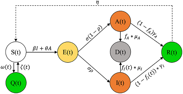
Figure 1. The SEAIRDQ compartmental model used in the present study. Individuals that are practicing social awareness (including social distancing, quarantine, shelter in place,...) are removed from the S compartment at a non-linear rate of ω(t) and are added to the quarantine (Q) compartment. On the contrary, changes in the quarantine observations are added back to the S compartment at a rate of ζ(t). In other words, parameters ω(t) and ζ(t) are polynomial functions that help in modeling the non-linear fluctuations of the susceptible compartment as the result of government orders, public awareness, and social distancing measures (Bakhtiari Ramezani et al., 2021).

3. Material and Methodology

3.1. Data

The number of daily death and reported confirmed infection cases were acquired at the county-level for each state from USA Facts (2020). This data was combined with county-level metrics (including each county's population) to get a fine level measure of the spread of the virus in each state. Aggregated county-level values were then used to model each state. Differential evolution was used to find the globally optimal solution by minimizing the errors between the observed cases and modeling outcomes.

Additionally, this study uses publicly available travel, mobility, and contact index data from Cuebiq (2020a,c). According to Lawrence (2019), location data collected from anonymous users who choose to share their location data with Cuebiq's mobile application partners are used to calculate the dwell time. The dwell time determines the length of stay of a mobile user at a particular location and the distances traveled by the user in a given period of time. We also use several of the metrics that Cuebiq has defined (Cuebiq, 2020b), as the basis of our correlation studies. These metrics include:

• Cuebiq Mobility Index (CMI): median of a derivative factor to indicate how far individuals have traveled each day. The CMI is expressed in a logarithmic scale, with a CMI of three indicating that the target study area's median users have traveled 1,000 m (or 1 km) that day.

• Cuebiq Contact Index (CCI): determines whether two or more devices have stayed within 15.2 m of each other over a five-minute period. It should be noted that individuals without a cellular device (such as students) or those who have not opted for their location information to be anonymously shared are excluded from these calculations.

• @Home or Shelter-In-Place (SIP): indicates the percentage of users with movements <100 m of movement in a day.

• Year over Year (YoY): indicated the variation of a metric (CMI, CCI, or SIP) relative to the mean of that metric over the past 365 days.

3.2. Methodology

As mentioned before, the goal of the present study is to study the effect of intrastate and interstate travels on the spread of COVID-19. It should be noted that modeling the nationwide travel effects necessitates the international travels into the US, along with the 2-weeks shelter-in-place (SIP) data to be included; however, such data was not accessible, and consequently, conducting a nationwide study was not possible.

As noted in section 3.1, due to privacy settings or availability of a cellular device, differences between the population trend captured through Cuebiq indices (such as SIP or CCI) and those estimated by the model [such as S(t), or Q(t)], are expected to exist. In order to examine the connection between epidemic and inter-state travel behavior:

1. The number of travelers from each of the 50 states to a target state was determined.

2. The number of individuals who traveled from another state and did not observe the 2-weeks shelter-in-place guideline (No-SIP) was determined.

3. To determine the probability of being exposed to infection among the No-SIPs, the compartmental model was run for each of the 50 states, and the probability of being exposed to infections was determined for travelers from each state.

4. To inform the model of realistic initial estimates for social awareness, the @Home (SIP) value of each state at the time of reporting of the first infectious case is used to set the lower bound for the initial social awareness or the quarantine compartment population (Q₀). The upper bound of Q₀ for that state is set to 99%, and a differential evolution model is then used to match the model's output with the reported cases.

5. Initial conditions (ICs) play an important role in the correct behavior of the ODEs and are one of the most prominent sources of bias in the calculations. To set the most realistic ICs:

• Model variables' bounds are chosen from reported values in the literature. If a parameter was not reported in the literature, Bayesian calibration and sensitivity analysis, as described in Bakhtiari Ramezani et al. (2021), were performed to ensure that the most suitable ranges were used.

• Differential evolution modeling is performed on the first 60 days of the data (i.e., cumulative infections and deaths) in each state.

• The trained model is used to estimate the correct ICs (A₀, S₀, Q₀, and E₀). These initial values are used to perform a history match for the whole observation period and further refine the match parameters.

6. For each day in the interstate modeling period, the daily travel data from each state is used to estimate the daily influx of exposed travelers from that state. These new exposures and the infections caused by previous travelers and otherwise normal rate of infections are used to determine the compounding effect on updated infections and deaths in the target state.

3.2.1. The Effect of Intrastate Mobility on Susceptibility

To study the correlation between intrastate mobility and susceptibility, we should first note that individuals are no longer susceptible to infection as they move to the Social Awareness compartment, Q(t). We should also note that the synchronicity of reported data (i.e., the lag between observed data and reported values) can adversely affect the results' interpretability.

Several factors affect the synchronicity of reported data and can introduce modeling biases. These may include the incubation period (the time it takes for the first symptoms to emerge), which is estimated to be between 5 and 7 days for COVID-19 (Jia et al., 2020; Volpatto et al., 2020; Bakhtiari Ramezani et al., 2021), the waiting period to be tested, and availability of the results (which was typically several days during the initial months of the pandemic outbreak), technical issues, laboratory errors, backlogs, and delay in entering the data into national databases. Consequently, the spread resulting from an event that happened at a particular date may not show itself in the data until several days later.

Additionally, since most students do not carry a cellular device to school, capturing the effect of school reopening through CCI is not readily available. To overcome this shortcoming and avoid any biases that can stem from this, we have limited the intrastate study period to the first few months following the first reported infection in the states (i.e., up until schools reopening).

3.2.2. Precautions for Travel—SIP

One of the important factors to consider while traveling from one state to another is to shelter in place for 14 days upon arrival at the destination. This section will examine the effect of interstate travel and evaluate the additional risk of infection that may be introduced as travel between the two regions takes place.

Due to the lack of high granularity data that would distinguish between the general travelers and infected travelers, using a multi-city compartmental model, such as the one suggested by Arino and van den Driessche (2003), is not possible; instead, we will examine the effect of mobility through a probability function that estimates the number of exposed travelers to a destination.

The probability of being exposed at any given date in any state is determined through the sum of all infected individuals (whether symptomatic or asymptomatic) at that date, divided by the total population of the state. Note should be taken that the number of infected individuals is not simply the number of positive cases reported at the date of interest, as this would not take the course of the illness or asymptomatic individuals into account. Instead, we will define the probability of being exposed or infected at time t, in the state s as P_s(t):

$\begin{array}{ll}{P}_s(t)=\frac{I_s(t)+A_s(t)}{N_s}& (1)\end{array}$

where I_s(t) and A_s(t) show the number of individuals at time t in the symptomatic and asymptomatic compartments in the state s, respectively, and N_s is the population of the state s.

The travelers' SIP data suggests that the majority of travelers (over 83.5%) have not adhered to the recommended SIP measures and have had displacements of more than 100 m in the first 14 days of their visit (Cuebiq, 2020c). It is important to note that the exposed individuals can spread the disease at a minimum rate of β(t) in the destination state, increasing the potential for the number of infections. As a result, the influx of inter-state travelers that fail to observe the SIP guidelines and adhere to them can pose a considerable risk of spikes in the number of cases.

It is unlikely that travelers suffering from COVID-19 symptoms, or those who have completed their incubation period, would leave for another (destination) state; as a result, we assume that travelers incoming to a destination state are merely exposed and have no initial symptoms, and will not exhibit any symptoms until their incubation period is completed, which as stated before is estimated to be between 5 and 7 days.

The product of P_s(t), Equation (1), for each state by the number of travelers per day from that state that have not observed SIP, n_s(t), gives the probable number of exposed or infected individuals that have traveled to the destination of interest on a single day:

$\begin{array}{ll}\delta E_T(t)={\displaystyle {\sum }_{s=1}^m}{P}_s(t)·n_s(t)& (2)\end{array}$

where δE_T(t) denotes the incrementally exposed individuals added to the destination state through travel and will show signs of infection following their incubation period, and m is the total number of states with travelers coming to the destination state. Each exposed traveler may become symptomatic infected or asymptomatic infected. These exposed travelers residing in the destination state and not observing SIP will expose other susceptible individuals in the destination, S(t), with the state's transmission rate, β(t), during their incubation period. Since the incubation period is between 5 and 7 days, a stacking effect will be observed; a new batch of exposed individuals traveling into the destination and not observing SIP will expose new susceptible individuals. In contrast, the previously exposed travelers will keep adding to the exposed individuals.

To accurately capture this compounding effect and complex chain of exposures and subsequent infections through travel, SEAIRDQ modeling is performed for all periods following travels, on a smaller scale model that uses the initial number of exposed travelers and the model parameters of the destination state. This incremental analysis allows for a complete breakdown of the spreading that results from travel vs. the normal course of infectious disease.

3.2.3. Model Calibration

Following Bakhtiari Ramezani et al. (2021), a Bayesian calibration study was conducted to minimize uncertainty in different modeling parameters and produce results that capture observed values of cumulative infection and death.

4. Case Study

Due to the lack of data on incoming international travels to the US, including the SIP data, this study has focused on state-level modeling and nationwide travels. A case study is conducted for Alabama to examine the correlation between intrastate and interstate mobility and contact indices with social awareness practices and examine the compounding effect of infections through exposed travelers.

We will study a baseline model, reflecting on the existing observations (including all interstate mobility trends), vs. an idealized case where inbound exposed travelers would follow SIP guidelines and self-quarantine for a minimum incubation period of 5–7 days.

4.1. Baseline Modeling

As pointed out in section 3, the correct selection of the initial conditions is critical to the ODEs. Published values and observations from mobility data were used to set the ICs and their lower/upper bounds. For example, the SIP value of 17% for AL on March 14, 2020, shows that S₀ is not the same as N, the state's total population. It should be noted that the majority of the compartmental models, except for Jia et al. (2020) and Bakhtiari Ramezani et al. (2021), take S₀ to be the same as N. The value of SIP is used as the lower bound of the initial social awareness compartment, Q₀.

4.1.1. Insights and Data

According to Division of infectious Diseases and Outbreaks (2020), several factors such as technical and laboratory errors, overcoming backlogs due to installation of new laboratory devices, and the likes, there are sudden spikes and inflation in the number of cases reported in Alabama. In order to better capture abnormalities seen in the reported data, data is analyzed in three time-segments:

• March 13, 2020–July 1, 2020

• July 1, 2020–September 1, 2020

• September 1, 2020–December 22, 2020

The cumulative number of infected individuals and deaths for Alabama is used to model each wave's peaks and starting date. Figure 2 shows the estimated symptomatic and asymptomatic infections, starting and end of SIP order and face mask mandatory order, as well as the starting date of the second and third waves in AL through December 22, 2020. Figure 3 shows a comparison between observed cumulative cases of infection and deaths in Alabama vs. those of the SEAIRDQ model. Table 1 shows a detailed comparison between estimated modeling results and the recorded cases for the state of Alabama from March 13, 2020, through December 22, 2020.

FIGURE 2

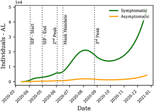
Figure 2. Distribution of the symptomatic and asymptomatic compartments using the SEAIRDQ model. Vertical lines show the starting and end of Shelter-In-Place (SIP) order and face mask mandatory order, as well as the starting date of the second peak and third peaks in AL through December 22, 2020.

FIGURE 3

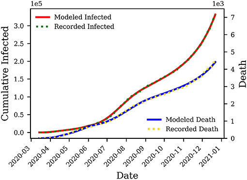
Figure 3. The cumulative infected and death cases reported vs. outputs of the SEAIRDQ model in Alabama. Accuracy of more than 99% for the confirmed infected cases, and over 98% for the deaths is observed, suggesting a close match and correctly calibrated model.

TABLE 1

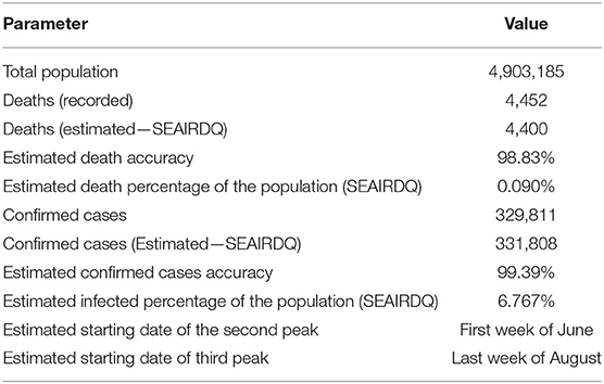
Table 1. Comparison between the recorded cases, and the outcome of the SEAIRDQ model for the state of Alabama through December 22, 2020.

4.2. Intrastate Mobility

A case study of intrastate mobility was conducted in Alabama; as noted in section 3.2.1, the intrastate mobility study is based on the first 5 months of data since initial infections were reported to avoid any bias introduced from schools reopening.

Figure 4 shows an example of the correlation study between the Q(t) compartment and the CCI in the state of Alabama. A strong inverse correlation of 98.7 between CCI and Q(t) is observed, with reporting lags of 24 days. This strong inverse correlation suggests that increased contact is inversely proportional to social awareness. It can also be observed that the SEAIRDQ model can capture the trends of social distancing (and, inversely, the contacts). This suggests that trends that are not necessarily observed through the contact metrics (such as the presence of students at schools) are also inherently captured by the model but cannot be further verified through CCI data alone.

FIGURE 4

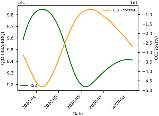
Figure 4. Correlation between CCI and Q(t) in Alabama for the 5 months proceeding the first reported case of infection in the state. A strong inverse correlation of 98.7 between CCI and Q(t) is observed, with reporting lags of 24 days, suggesting that the SEAIRDQ model can capture the trends of social distancing.

A similar study was conducted for increased intrastate mobility (i.e., increase in CMI YoY within a state) and Q(t); however, a strong correlation between the degree of mobility and susceptibility was not observed. This suggests that social awareness is not necessarily affected by mobility alone. As long as social distancing or other contact-related precautions are followed, travel will not directly influence susceptibility.

4.3. Interstate Mobility

The interstate travel with SIP measurement is publicly available on the Cuebiq website from September 28, 2020, through December 22, 2020. For this reason, we have used this available period to study the inter-state travel on the spread of COVID-19. Cuebiq reports travelers' data over 14 days; thus, overall data are divided by 14 to estimate the number of travelers per day. Figure 5 shows the average inter-state travels to Alabama from other states over this period.

FIGURE 5

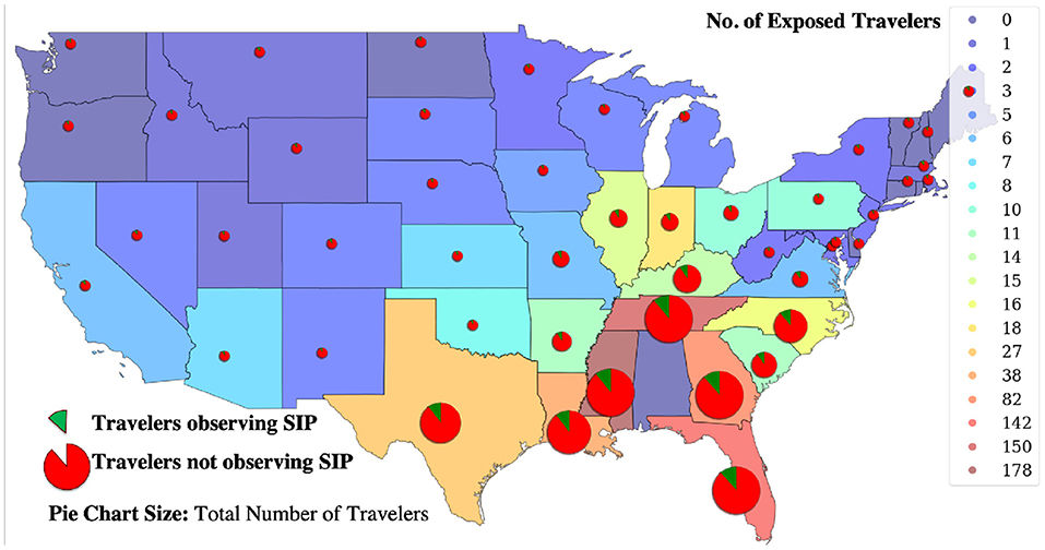
Figure 5. Average travels to Alabama and the percentage of SIP and No SIP for each origin state. The pie charts' size shows the number of travelers from each state to Alabama during the 83 days study period. Divisions of the pie chart reflect the percentage of SIP and No-SIP travelers. Individuals observing SIP are shown as green, and No-SIP individuals are denoted in red. The color scale of each state denotes the number of exposed travelers from that state. This number is determined by the probability of being exposed in the origin state at the end of 83 days of study (SIP and travel data from Cuebiq, 2020c).

The total number of interstate travelers from all states to Alabama shows 87.886 Million individuals over these 83 days with a 14-day window, averaging 75.6 thousand travelers per day, or an equivalent of 1.5% of the total population of Alabama. This means that the total travel volume to this state over the short span of 83 days is approximately 1.28 times the state's total population; thus, travel and its likelihood of amplifying the transmission cannot be ignored.

As discussed in section 3.2.2, incremental SEAIRDQ modeling is performed for each day after September 28, 2020 (the first day for which travel data is available). For each day of modeling, Equation (2) is used to estimate the daily flow of exposed individuals (yet to become fully infected) into the destination state. The total number of exposed individuals is subsequently used for E₀. Furthermore, Q₀ is taken to be zero, while I₀, and A₀ are both set to an initial seed value of one. The rest of the ICs from Alabama are used in the SEAIRDQ model for time t.

Figure 6 shows a comparison between the current symptomatic and asymptomatic infections in Alabama, reflecting the compounded effect of travels, vs. a model in which no travelers from other states were included in the model. As suggested by this figure, a considerable reduction of 53.9%, or 26, 255 individuals, could have been observed in the number of active infections if travelers from other states observed the SIP practices.

FIGURE 6

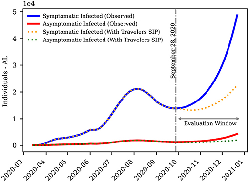
Figure 6. Effect of exposed travelers on the daily number of symptomatic and asymptomatic infections in Alabama. A reduction of 53.9%, or 26, 255 active infections, could have been observed if travelers from other states observed the SIP practices.

Figures 7, 8 show the outcome of the SEAIRDQ model on incremental travels. As noted in Figure 7, assuming that symptomatic individuals will quarantine, a potential decrease of 22.95% or roughly 76, 100 fewer infected cases could have been observed in Alabama, given all travelers from higher-risk states were to SIP for a minimum of their incubation period (5–7 days). On a similar note, according to Figure 8, cumulative death would have been reduced by 22.43%, or 989 people, if the same considerations were made.

FIGURE 7

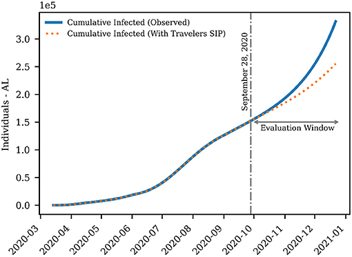
Figure 7. Effect of exposed travelers on cumulative infected individuals estimated using SEAIRDQ in Alabama. A potential decrease of 22.95% or roughly 76, 100 fewer infected cases could have been observed in Alabama, given all travelers from higher-risk states were to SIP for a minimum of their incubation period (5–7 days).

FIGURE 8

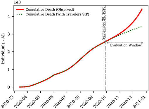
Figure 8. Effect of exposed travelers on the number of deaths in Alabama. Cumulative death would have been reduced by 22.43%, or 989 people if all travelers from higher-risk states were to SIP for a minimum of their incubation period (5–7 days).

5. Conclusion

A compartmental metapopulation model was used in the present study to analyze the correlation between social awareness compartment, Q, and contact index, CCI. It was observed that a strong inverse correlation exists between the contact index and social awareness and that the SEAIRDQ model can capture these correlations accurately. A similar correlation could not be established between Q and mobility index; this suggests that mobility by itself is not a defining factor for the spread of the disease, as long as the social distancing measures are observed. While the compartmental model was capable of capturing Q, even after school opening and ease of restrictions, lack of contact data for students and other social sectors has resulted in less apparent correlations, suggesting that CCI alone is insufficient to capture relaxation of social awareness measures. A probabilistic model was also created to estimate the number of exposed individuals traveling from other states to a destination state. Subsequent incremental modeling of travels to the destination state suggested that as much as 22% reduction in cumulative infections and deaths could be achieved, solely by observing SIP measures by travelers from other states.

Data Availability Statement

The raw data supporting the conclusions of this article will be made available by the authors, without undue reservation.

Author Contributions

SB, AA, and SR created the SEAIRDQ model, performed data acquisition, writeup and modeling. AP reviewed the work. MH, JP, PP, and XQ provided support in the present study. All authors contributed to the article and approved the submitted version.

Conflict of Interest

The authors declare that the research was conducted in the absence of any commercial or financial relationships that could be construed as a potential conflict of interest.

References

Arino, J., and van den Driessche, P. (2003). A multi-city epidemic model. Math. Popul. Stud. 10, 175–193. doi: 10.1080/08898480306720

PubMed Abstract | CrossRef Full Text | Google Scholar

Bakhtiari Ramezani, S., Amirlatifi, A., and Rahimi, S. (2021). A novel compartmental model to handle the nonlinear trend of COVID-19 epidemic. J. Comput. Biol. Med.

Belik, V., Geisel, T., and Brockmann, D. (2011). Natural human mobility patterns and spatial spread of infectious diseases. Phys. Rev. X 1, 1–5. doi: 10.1103/PhysRevX.1.011001

CrossRef Full Text | Google Scholar

CDC (2020). First Travel-Related Case of 2019 Novel Coronavirus Detected in United States. CDC.

Google Scholar

Chatterjee, S., Sarkar, A., Chatterjee, S., Karmakar, M., and Paul, R. (2020). Studying the progress of COVID-19 outbreak in India using SIRD model. Indian J Phys Proc Indian Assoc Cultiv Sci. doi: 10.1007/s12648-020-01766-8. [Epub ahead of print].

PubMed Abstract | CrossRef Full Text | Google Scholar

Cuebiq (2020a). Cuebiq Contact Index Trend. Available online at: https://public.tableau.com/profile/fabio.baraghini#!/vizhome/CMI-2_0/CI

Cuebiq (2020b). Cuebiq's COVID-19 Mobility Index (CMI). Available online at: https://help.cuebiq.com/hc/en-us/articles/360041285051-Cuebiq-s-COVID-19-Mobility-Index-CMI

Cuebiq (2020c). Travelers Shelter-In-Place. Available online at: https://public.tableau.com/profile/fabio.baraghini#!/vizhome/CMI-2_0/SIPTravelers

Division of infectious Diseases and Outbreaks (2020). Daily Number and Moving Averages of Cases by Date of Report (Statewide). Available online at: https://alpublichealth.maps.arcgis.com/apps/opsdashboard/index.html#/6d2771faa9da4a2786a509d82c8cf0f7

Dong, E., Du, H., and Gardner, L. (2020). An interactive web-based dashboard to track COVID-19 in real time. Lancet Infect. Dis. 20, 533–534. doi: 10.1016/S1473-3099(20)30120-1

PubMed Abstract | CrossRef Full Text | Google Scholar

Du, Z., Wang, L., Cauchemez, S., Xu, X., Wang, X., Cowling, B. J., et al. (2020). Risk for transportation of coronavirus disease from Wuhan to other cities in China. Emerg. Infect. Dis. 26, 1049–1052. doi: 10.3201/eid2605.200146

PubMed Abstract | CrossRef Full Text | Google Scholar

Fernández-Villaverde, J., and Jones, C. (2020). Estimating and Simulating a SIRD Model of COVID-19 for Many Countries, States, and Cities. Technical report, National Bureau of Economic Research, Cambridge, MA. doi: 10.3386/w27128

CrossRef Full Text | Google Scholar

Jia, J., Ding, J., Liu, S., Liao, G., Li, J., Duan, B. E., et al. (2020). Modeling the control of COVID-19: impact of policy interventions and meteorological factors. Electron. J. Differ. Equat. 2020, 1–24.

Google Scholar

Kraemer, M. U. G., Yang, C.-H., Gutierrez, B., Wu, C.-H., Klein, B., Pigott, D. M., et al. (2020). The effect of human mobility and control measures on the COVID-19 epidemic in China. Science 368, 493–497. doi: 10.1126/science.abb4218

PubMed Abstract | CrossRef Full Text | Google Scholar

Lawrence, C. (2019). Cuebiq on Location Data Advancements and How Privacy Plays a Role. Adelphic.

Lingzhi, M., Bouardi, H. T., Lami, O. S., Trichakis, N., Trikalinos, T., Zarandi, M. F., et al. (2020). Overview of DELPHI Model. Technical Report April, Massachusetts Institute of Technology.

Moghadas, S. M., Shoukat, A., Fitzpatrick, M. C., Wells, C. R., Sah, P., Pandey, A., et al. (2020). Projecting hospital utilization during the COVID-19 outbreaks in the United States. Proc. Natl. Acad. Sci. U.S.A. 117, 9122–9126. doi: 10.1073/pnas.2004064117

PubMed Abstract | CrossRef Full Text | Google Scholar

Pei, S., Kandula, S., and Shaman, J. (2020). Differential effects of intervention timing on COVID-19 Spread in the United States. Science Advances 6:eabd6370. doi: 10.1126/sciadv.abd6370

PubMed Abstract | CrossRef Full Text | Google Scholar

Pei, S., Kandula, S., Yang, W., and Shaman, J. (2018). Forecasting the spatial transmission of influenza in the United States. Proc. Natl. Acad. Sci. U.S.A. 115, 2752–2757. doi: 10.1073/pnas.1708856115

PubMed Abstract | CrossRef Full Text | Google Scholar

USA Facts (2020). USA Facts - US Coronavirus Cases and Deaths. Available online at: https://usafactsstatic.blob.core.windows.net/public/data/covid-19/covid_confirmed_usafacts.csv

Volpatto, D., Resende, A. C., dos Anjos, L., Silva, J., Dias, C., Almeida, R., et al. (2020). Spreading of COVID-19 in Brazil: impacts and uncertainties in social distancing strategies. medRxiv. doi: 10.1101/2020.05.30.20117283

CrossRef Full Text | Google Scholar

Wang, X., Du, Z., Pasco, R., Pierce, K., Petty, M., Fox, S. J., et al. (2020). COVID-19 Healthcare Demand Projections: Austin, Texas. Technical report, The University of Texas at Austin, Austin, TX.

Google Scholar

Wells, C. R., Sah, P., Moghadas, S. M., Pandey, A., Shoukat, A., Wang, Y., et al. (2020). Impact of international travel and border control measures on the global spread of the novel 2019 coronavirus outbreak. Proc. Natl. Acad. Sci. U.S.A. 117, 7504–7509. doi: 10.1073/pnas.2002616117

PubMed Abstract | CrossRef Full Text | Google Scholar

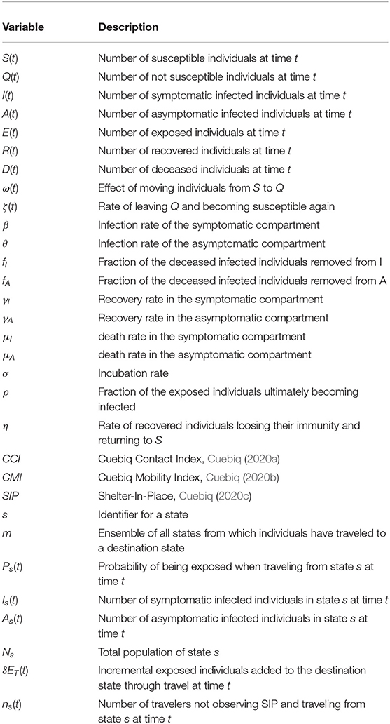
6. Nomenclature