Estimation of Traffic Flow Rate With Data From Connected-Automated Vehicles Using Bayesian Inference and Deep Learning

Connected automated vehicles (CAVs) hold promise to replace current traffic detection systems in the near future. However, traffic state estimation, particularly flow rate, poses a major challenge at low CAV penetration rates without other supporting infrastructure of sensors. This paper proposes flow rate estimation methods using headway data from CAVs. Specifically, Bayesian inference and deep learning based methods are developed and compared with a naïve method based on a simple arithmetic mean of observed headways. The proposed methods are investigated via numerical experiments to evaluate their performance with respect to the CAV penetration rate, traffic demand, and availability of historical data. The methods are further validated with real data. The results show that the Bayesian inference based method, which estimates the flow rate distribution by integrating current (real-time) data and previous knowledge, can perform well even at low penetration rates with good prior information. However, in high CAV penetration, its relative advantage to the other methods diminishes because the prior information always influences the flow rate estimation. The deep learning based method can be effective with a large amount of data to train the model; however, in low CAV penetration, it tends to converge to the mean of target output values regardless of the observed data. At last, in relatively high CAV penetration, the relative advantage of the advanced methods is negligible and in fact, the naïve method is preferred in terms of accuracy as well as efficiency.

Introduction

Traffic data collected by various detector systems is fundamental to traffic operations. Conventional detectors, such as inductive loop detectors, typically provide vehicle speed, flow rate, and occupancy at fixed locations, and traffic states can be estimated using these data. On the other hand, connected-automated vehicles (CAVs) are expected to be on our roads in the near future and fundamentally change how we sense and control traffic. CAVs can collect detailed and accurate data about themselves and the surrounding vehicles through advanced sensing, and they can share these high-resolution data in real time through V2V (vehicle-to-vehicle) or V2I (vehicle-to-infrastructure) communication. Since CAVs can collect and provide traffic data, they can replace the current infrastructure-based detector systems which are costly to install and maintain. Recognizing this potential, a number of advanced concepts of traffic control using CAVs have emerged in recent years (Hegyi et al., 2013; Roncoli et al., 2015; Han et al., 2017; Han and Ahn, 2018).

In early stages of CAV adoption, traffic data may be obtained from both traditional detectors and CAVs. However, with the high cost of detector maintenance, there may be desire for agencies to phase out traditional detectors quickly if CAV data alone can provide sufficient information. Furthermore, in many areas, detector coverage is not sufficient enough to estimate traffic states with reasonable accuracy. Thus, deriving traffic information mainly using CAV data could reduce reliance on traditional sensors and extend the data collection coverage. The initial low penetration rate of CAVs, however, is a significant obstacle to obtain reliable traffic information. To overcome this, various methods to estimate traffic states using limited data from CAVs, connected vehicles (CVs), or probe vehicles have been widely developed in the literature (Seo et al., 2017). For example, Bekiaris-Liberis et al. (2016) presented a macroscopic model-based approach to estimate density and flow rates in mixed traffic of conventional and connected vehicles. They used data of the average speed of CVs, assuming that it is similar to the average speed of the entire traffic flow, and a total flow rate from conventional detectors. The proposed method was validated via microscopic simulation considering a low penetration rate of CVs (Fountoulakis et al., 2017). Later, Bekiaris-Liberis et al. (2017) also developed a traffic state (per-lane density, on-ramp and off-ramp flows) estimation method using CV data with total flow from fixed detectors. This method was evaluated in microscopic simulation with NGSIM data (Papadopoulou et al., 2018). While these previous studies demonstrate satisfactory estimation of traffic states in low penetration of CVs, they still require conventional detectors, particularly for flow rate, albeit fewer than what the current detecting system requires.

On the other hand, Seo et al. (2015) developed a flow and density estimation method based on the Edie’s generalized definitions (Edie, 1963) only using data from probe vehicles that have ability to detect spacing with its leading vehicle. They performed a field experiment with 20 probe vehicles and verified that the proposed method could effectively capture important traffic dynamics such as queue propagation, even at a very low penetration rate of probe vehicles. Similarly, Seo and Kusakabe (2015) developed a method to estimate traffic states from probe vehicle data using the flow conservation law. They estimated the number of vehicles between two neighboring probe vehicles based on their average headways (over distance) with their respective leaders (non-probe vehicles) and the average time (over distance) interval between the probe vehicles. These methods clearly present the possibility of using CAV-only data to estimate traffic states, and the simple conservation law enhances the accuracy without any exogenous assumptions such as a fundamental diagram. However, they assumed that the relationship between a probe vehicle and its leading vehicle represents the traffic state at large, and therefore, significant error is expected when the headway deviation among vehicles is large, particularly in free-flow traffic. Thus, reliable estimation of traffic states, particularly flow rate, only using CAVs remains a major challenge.

The methods introduced above are grounded on sound traffic flow theory. Nevertheless, they show limitations in their performance or applications largely due to their limited ability to capture complex features in the traffic data. On the other hand, state-of-the-art data-driven methods have emerged to address feature complexity and to overcome data scarcity. Among them, Bayesian inference is a pioneering method in Statistics to derive results particularly when data is limited. This method estimates a conditional distribution on the observed data by integrating prior knowledge. In traffic engineering, Bayesian methods are widely used to estimate capacity (Ozguven and Ozbay, 2008), travel time (Jintanakul et al., 2009; Fei et al., 2011; Hofleitner et al., 2012), or traffic state (Neumann et al., 2013; Kim and Wang, 2016). Since traffic exhibits recurrent daily patterns, past traffic information can complement limited real-time data from CAVs. Thus, Bayesian inference is a good candidate method to estimate traffic states in a CAV environment. Nonetheless, research in this regard is largely missing in the current literature.

Another promising data-driven method is machine learning algorithms, such as deep learning. Despite its inability to provide physical insight, a notable advantage of deep learning is that it can capture complex features of data to describe a target value even if the relationship is nonlinear and too complex to describe by conventional methods. In traffic engineering, deep learning is widely used in many areas such as vehicle behavior modeling (Wei et al., 2010; Khodayari et al., 2012; Mathew and Ravishankar, 2012; Zheng et al., 2013; Papathanasopoulou and Antoniou, 2015; Simonelli et al., 2015; Lefevre et al., 2016; Motamedidehkordi et al., 2017; Zhou et al., 2017) and future traffic state predictions (Ma et al., 2015; Fusco et al., 2016; Julio et al., 2016; Polson and Sokolov, 2017). For example, Polson and Sokolov (Polson and Sokolov, 2017) developed a deep learning architecture for short-term flow prediction. The proposed model was validated with loop-detector data in the Chicago area and showed reliable prediction performance in capturing nonlinear changes of flow rate. Clearly, deep learning has the huge potential to link (sparse) CAV data to traffic states at large, but its potential has not been fully explored, including estimation and prediction of flow rate.

Based on the above review, we find that advanced data-driven methods have the potential to provide better estimation and prediction capabilities. However, a systematic investigation into their advantages and their limitations for traffic flow estimation is currently lacking. To this end, this paper aims to address 1) whether promising data-driven methods can be used to estimate traffic states, more specifically flow rates in free-flow traffic, using sparse CAV data; 2) how these methods perform in different traffic conditions (e.g., demand, CAV penetration rate); and 3) how much better these methods can perform compared to the simple average approach. Specifically, we consider three methods: 1) a naïve method that relies only on the observed CAV data as a baseline, 2) Bayesian inference based method that integrates real time CAV data and historical traffic data, and 3) deep learning based method that extracts complex relations between CAV headways and traffic state directly from large amount of data. This paper evaluates three methods through numerical experiments and validates them with real data. The evaluation results show how the performance of each model fares against others in different traffic situations (e.g., different flow rates, CAV penetration rates, etc.), casting light on in what situation each method should be preferred.

Note that we focus on estimating the flow rate in free-flow states because it is an important indicator for predicting traffic breakdown (Elefteriadou et al., 1995; Persaud et al., 1998; Han and Ahn, 2018). A major challenge is that in a free flow state, vehicle headways (both conventional vehicles and CAVs) are distributed randomly due to the randomness in vehicle arrivals (i.e., dictated by the demand). Therefore, partial CAV headway data may not represent the flow rate of traffic at large. On the other hand, in a congested state, vehicle headways show less variation as vehicles are constrained, and random arrivals are much less likely. Thus, we expect partial CAV headways to represent the flow rate better in congested traffic. In addition, speed estimation from CAV data is more straightforward as the partial CAV speed is similar to the traffic speed (Elfar et al., 2018). However, speed does not vary significantly in free-flow traffic and thus, is not a good indicator for predicting traffic breakdown.

The main findings of this paper are as follows. The proposed Bayesian inference based method can show good performance even at a low CAV penetration rate (< 20%) due to its reliance on prior (historical) information. However, as the CAV penetration or demand increases, its relative advantage to the other methods (a deep learning based method and even a simple average) wanes since the prior information will always influence the flow rate estimation. Particularly, in high CAV penetration, where real-time CAV information alone suffices for accurate flow estimation, inclusion of prior information can actually hinder the accuracy. The narrower the prior distribution is, the stronger the influence of prior information would be for flow estimation. In contrast, the deep learning based method is effective for estimating the flow rate using only CAV data when the CAV penetration rate is moderate to high (>20%). However, when the data is sparse (in light traffic or low penetration), the method produces an estimate close to the mean of the training data regardless the observed real-time data. Finally, at a relatively high CAV penetration rate (>70%), the relative advantage of the advanced methods is negligible, and in fact, the naïve method is preferred in terms of accuracy as well as efficiency.

This paper consists of five sections. Methods describes the proposed methods, and Numerical Experiment describes the numerical experiments to investigate the features of each method in various traffic conditions. In Validation With Real Data, the methods are validated with real data, and conclusion and discussion are provided in Section Conclusion and Discussion.

Methods

This section presents methods that estimate a flow rate using CAV data. Firstly, we assume a CAV will share its own state (e.g., location, speed) with roadside infrastructure and also measure surrounding vehicles (e.g., spacing, relative speed) through its sensors. In this context, we consider that the following data are available over time from CAVs, as illustrated in Figure 1.

Location, $l$, and Speed, $v$, of CAV.

Spacing between CAV and its leading vehicle, $s$.¹

FIGURE 1

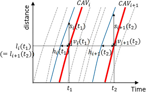
FIGURE 1. Illustration of available data from CAVs over time.

For simplicity, we also assume the data from CAVs have negligible error. Using these data, we can easily estimate (time) headway between a CAV and its leading vehicle, $h \left(=s/v\right)$. And, using headway data in a certain time interval, $T$, a flow rate will be estimated through the proposed methods in the following subsections². We assume that CAV data can be collected continuously over time and location, and thus, the flow rate can be estimated in the entire time-space domain.

Method 1: Naïve Method (Baseline)

The first method is the simplest but naïve method that relies only on observed CAV data. Other traffic information is assumed unavailable. This method will serve as the baseline to evaluate the performance of the more advanced methods, methods 2 and 3. In this method, the arithmetic mean of headways is used to estimate a flow rate, $\widehat{q}$, expressed as:

$\widehat{q}=E{\left(h\right)}^{-1}={\left(\frac{{\displaystyle {\sum }_{i=1}^N{h}_i}}{N}\right)}^{-1}(1)$

where $h_i$ is the headway between $i^{\text{th}}$ CAV and its leading vehicle, and $N$ is the number of CAVs in the time interval, $T$. Then, the standard error of $E\left(h\right)$, ${\sigma }_{E\left(h\right)}$, is

${\sigma }_{E\left(h\right)}=\frac{\delta }{\sqrt{N}}(2)$

where $\delta$ is the standard deviation of headway for all vehicles, including CAVs and conventional vehicles. Equation 2 shows that this method is affected by 1) traffic state, 2) penetration rate of CAVs, and 3) time interval, $T$: the estimated flow rate would not be precise when $\delta$ is large (e.g., in a free flow state) or $N$ is small (e.g., a low CAV penetration rate or small $T$).

Method 2: Bayesian Inference

In many instances, some historical traffic data can be available (from multiple days to years). This historical data could provide some sense of traffic state for certain time and location. Alone, it is obviously not adequate for traffic state estimation due to daily variations, but when combined with real-time data, it can improve the accuracy of traffic state estimation. In Statistics, Bayesian inference has been developed to systematically integrate a (limited) real time data and (related) other information. In a similar context, we develop a Bayesian inference based method to estimate flow rates using real time CAV data and distribution of flow rate from historical data set.

Specifically, this method derives a posterior probability distribution of flow rate with respect to the observed headways, $p\left(q|h\right)$, with a prior probability of flow rate, $p\left(q\right)$, and a likelihood function of flow rate and headway, $p\left(h|q\right)$, using Bayes’ theorem:

$p\left(q|h\right)=\frac{p\left(q\right)\times p\left(h|q\right)}{p\left(h\right)}=\frac{p\left(q\right)\times {\displaystyle {\prod }_{i=1}^{N}p\left(h_i|q\right)} }{{\displaystyle \int p\left(q\right)}\times {\displaystyle {\prod }_{i=1}^{N}p\left(h_i|q\right)} \text{d}q}(3)$

Note that the denominator is a normalizing factor to ensure that the sum of the posterior distribution equals to one. Thus, for simplicity, $p\left(q|h\right)$ can be written as,

$p\left(q|h\right)\propto p\left(q\right)\times p\left(h|q\right)=p\left(q\right)\times {\displaystyle {\prod }_{i=1}^{N}p\left(h_i|q\right)}(4)$

Notably, to estimate $p\left(q|h\right)$ by Bayesian inference, more information of $p\left(q\right)$ and $p\left(h|q\right)$ are required. Firstly, $p\left(q\right)$ represents a prior distribution of flow rate before collecting current headway data. As stated earlier, the flow rate is expected to fluctuate over time but exhibit similar daily patterns (e.g., typical AM or PM rush hour). Thus historical flow rate data for the same time of the day (and the same day of the week) would be the most reasonable choice for prior information. Note that for the prior data (and training data for Method 3), getting historical data could be a main constraint for adopting these methods. Data from existing detectors can be used if available, but additional surveying would be required if no existing data or detectors are available. Historic estimation results based on previous CAV data can be used, though there will be some transition period until sufficient data become available. Nevertheless, using CAV data with the proposed methods could reduce the efforts to collect traffic data and could estimate traffic states even in the areas without any detectors. A likelihood function represents the headway distribution with respect to flow rate. Field observations can be used to estimate this function, though this has been widely studied in the literature [see (Li and Chen, 2017) for a recent review].

These model features suggest that the estimation results will depend on the prior information. Specifically, the estimation results would suffer when the prior information provides little information (e.g., a very wide prior distribution), constrains too much (e.g., a very narrow prior distribution), or differs from the true value significantly (e.g., distinct flow rate from prior distribution). In Sections Numerical Experiment and Validation With Real Data, we will verify these features more systematically through numerical experiments and validation with real data, and provide some insight when we should expect the Bayesian inference based model to perform well or poor.

Method 3: Deep-Learning Based Method

With advancement of data processing techniques, more data-driven methods such as deep learning have been widely developed. Unlike the Bayesian approach, which requires both fundamental knowledge of traffic flow (for the likelihood function) and existing data (for the prior distribution), deep learning aims to extract outcomes (e.g., traffic flow) directly from data without relying on a physical model. Deep learning has been applied in a wide variety of disciplines due to its high accuracy when it is trained by a large amount of data, though it does not provide physical insights. Therefore, in this study, we propose a deep learning based method to estimate the flow rate directly from CAV data. Note that, in a free flow state, especially in a low CAV penetration rate, the relationship between the observed CAV data and flow rate cannot be easily described by a physical model due to the randomness in vehicle arrivals. Thus, a data-driven method, such as the one proposed in this paper, may be more effective in capturing the complex relationship.

Figure 2 presents the architecture of the proposed deep learning based method with two hidden layers (with ten nodes) and one output layer (with one node). Note that we use two hidden layers as we found during a numerical experiment that the model performance does not improve significantly with more hidden layers. Nonetheless, the architecture can be modified based on the data properties without changing the proposed framework. To train the model, initially, the input data of CAV headways, $\mathit{h}=\left(h_1, h_2,\dots ,h_N\right)$, are connected to each node in the first hidden layer through the weight matrix of ${\mathit{W}}^1=\left\{w_{\mathrm{1,1}}^1,\dots ,w_{10,N}^1\right\}$. Each node generates net input ${\mathit{n}}^1$, with bias ${\mathit{b}}^1$, and ${\mathit{n}}^1$ will be transformed to output vector ${\mathit{a}}^1$ through activation function $f^1$, as presented in the figure. Then ${\mathit{a}}^1$ becomes the input vector to the second hidden layer, and same process is repeated to generate ${\mathit{a}}^2$. The output layer has only one node that generates ${\mathit{n}}^3$, which will be transformed to a final output vector for estimated flow rates, $\widehat{\mathit{q}}$, via activation function $f^3$. The activation functions in the two hidden layers, $f^1$ and $f^2$, are rectified linear unit (ReLU) functions and the activation function in the output layer, $f^3$, is a linear function for scaling. The output vector of $\widehat{\mathit{q}}=\left({\widehat{q}}_1,\dots , {\widehat{q}}_M\right)$, where $M$ represents the number of datasets for training, will be compared with the target vector of $\mathit{q}$, the ground-truth, to tune the weights and biases through backpropagation algorithm (Rumelhart et al., 1986) that aims to minimize the objective function of mean square error (MSE), expressed as:

$\text{MSE}=\frac{{{\displaystyle {\sum }_{m=1}^M\left(q_m-{\widehat{q}}_m\right)}}^2}{M}(5)$

FIGURE 2

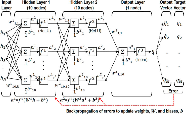
FIGURE 2. Architecture of the proposed Deep-learning method [Reconstructed from (Beale et al., 2015) and (Jun et al., 2017)].

After training, this model can estimate flow rates with a new set of headway data. Notably, the deep learning based model does not require any assumptions for traffic flow properties such as the likelihood function in the Bayesian approach. However, as we will show later, its accuracy is close to and sometimes better than the accuracy of the Bayesian approach. Note that for the proposed deep learning based method, we used a simple “vanilla” neural network with the assumption that there is no specific relationship between the order of headways and the flow rate since CAVs are randomly distributed in traffic flow. If the headway sequence is deemed significant, though unlikely in most foreseeable conditions, Recurrent Neural Network (RNN) or Long Short Term Memory (LSTM) Networks would be more suitable to estimate the flow rate. More discussion on deep learning application will be provided in the conclusion.

In the following sections, we will investigate the features of deep learning based method in detail and verify that this method can be effective for estimating the flow rate using only observed CAV data. However, when the relationship between the flow rate and CAV data are too weak (e.g., light traffic or a low CAV penetration rate), this method fails to provide meaningful results as it only aims to minimize the objective function (Eq. 5). The detailed results and insights will be presented later.

Numerical Experiment

Numerical Experiment Set-Up

To investigate the features of proposed methods, we conduct a numerical experiment in this section. For the headway data, we generate 1,000 data sets that include 100 headways for each, and each headway is randomly generated from an exponential distribution with a mean of 1.8 s (equivalent to a flow rate of 2,000 veh/hr). The cases for light and heavy traffic demand are also investigated in Section Effects of Traffic Demand on Flow Rate Estimation. Note that, we use an exponential distribution to generate random vehicle arrivals in a free flow state, but it can be changed to any distribution. The actual flow rate for each data set can be derived as a reciprocal of the mean of the 100 headways, and the 1,000 data sets represent a wide range of flow rates as illustrated in Figure 3A. Note that by the central limit theorem, the mean of the 100 headways will be approximately normally distributed with the mean of 1.8 s (the population mean) and the standard error of $0.18\left(=1.8/\sqrt{100}\right)\text{s}$. Among the 100 headway data in each data set, we randomly select headways according to the assumed penetration rate of CAVs. For example, if the penetration rate is 30%, 30 headways are used in each data set to estimate a flow rate.

FIGURE 3

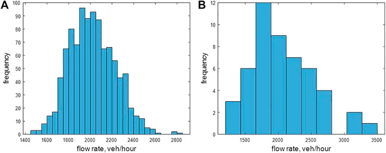
FIGURE 3. Examples of flow rate histogram (A) actual flow rate; (B) flow rate from prior distribution.

For the Bayesian inference method, additional information on the prior distribution, $p\left(q\right)$, should be defined. We consider that historical flow rates are described by a bell-shaped gamma distribution with the mean of 2,000 veh/hr and the standard deviation of 500 veh/hr to represent typical traffic features recurrent daily patterns. We assume a relatively large deviation for the initial experiment to represent a less optimistic scenario of limited prior information, but a sensitivity analysis for smaller and larger standard deviations is also conducted in Section Effects of Prior Distribution on Flow Rate Estimation. The example of 50 flow rates from the assumed prior distribution is illustrated in Figure 3B. The figure shows that the historical flow rates are more concentrated near the true mean of 2,000 veh/hr, but the range is quite large (e.g., 1,200–3,500 veh/hr), which makes it unsuitable for real-time flow rate estimation. Instead, in the Bayesian inference based method, this prior distribution will be updated with real-time CAV data for more accurate flow rate estimation. The likelihood function of headway for given flow rate, $p\left(h|q\right)$, is assumed as exponential distribution to characterize random vehicle arrivals in a free flow traffic.

For the deep learning based method, we divide 1,000 data sets into three groups: 70% for training, 15% for validation, and 15% for test.³ The validation data set is used as an extension of training to avoid overfitting and improve generalization (Piotrowski and Napiorkowski, 2013). After training, the test data set is used to estimate flow rates. Note that 150 estimated flow rates are compared against the ‘‘ground truth’’ for deep learning based method, while 1,000 flow rates are estimated and evaluated for other methods.

Overall Results and Findings

Figures 4A–C present scatter plots of ground-truth (x-axis) vs. estimated (y-axis) flow rates by each method with different CAV penetration rates (10–70%), and Figure 4D shows the root mean square error (RMSE) for each case. Note that we present RMSE instead MSE to get a better sense of error in flow rate estimation. When the penetration rate of CAV is relatively high (>70%), all three methods perform well, but at a low penetration rate (10%), each method shows different features.

FIGURE 4

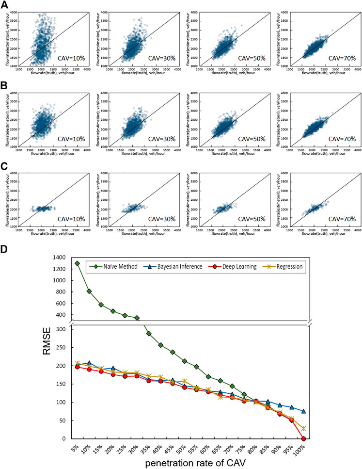
FIGURE 4. Results of numerical experiment: (A) Naïve method; (B) Bayesian inference; (C) Deep-learning; (D) RMSE vs. CAV penetration rate for each method.

The baseline, naïve method, as expected, shows dispersive results in low CAV penetration as presented in the left side of Figure 4A: the estimated flow rate exhibits a wide range of 1,000–4,000 veh/hr although the actual flow rate is within 1,500–2,500 veh/hr. This is due to the fact that the headways from CAVs at a low penetration rate have a large deviation, leading to estimate with low accuracy and precision as evidenced by a large RMSE value in Figure 4D.

The methods based on the Bayesian inference (Figure 4B) and deep learning (Figure 4C) present different features. Compared to the naïve method, the results from the Bayesian inference show the tendency, though scattered, to follow the reference line even at a low CAV penetration rate. This feature can be explained by the process of Bayesian inference, which reflects the information from both observed data (through the likelihood function) and distribution of historical ground truth (through the prior distribution): the probability of flow rate is initially determined by the prior distribution but gets updated with observed headways. Figure 5 presents an example to better illustrate the process. In this example, the actual flow rate (from 100 headways) is 2,375 veh/hr as marked by the left (red) dashed vertical line, and ten headways are available (10% penetration), with a mean of 1.06 s. Before updating with CAV data, we initially have a prior distribution, as represented by the left-most (black) curve. Note that, as assumed above, the prior distribution is a gamma distribution with a mean of 2,000 veh/hr and the deviation of 500 veh/hr. With CAV headways, we can derive a likelihood function as represented by the right-most (blue) curve. Notably, the likelihood function only contains the information from CAV data, and its mode (3,399 veh/hr) is same as the estimation by the naïve method. In the Bayesian process, we derive a posterior distribution for flow rate by incorporating the prior distribution and the likelihood function using Eq. 4: see the middle (orange) curve in Figure 5. In this example, the posterior mean is 2,467 veh/hr, and the mode is 2,376 veh/hr, both of which are closer to the actual flow rate than the prior information or observed data (naïve method).

FIGURE 5

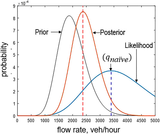
FIGURE 5. Example of Bayesian inference process.

In contrast, at a low CAV penetration rate (10%), the deep learning based method generates estimated flow rates around 2,000 veh/hr (the mean of the ground-truth) regardless the observed data (see the left-most in Figure 4C). This feature is inherent to the deep learning process as presented in Figure 2. Deep learning seeks to determine the weights and biases in the hidden layers that minimize the objective function. When the relationship between the input data (observed headways) and the target value (flow rate) is weak due to a large variation in the input data, the learning process decides that the weights are close to zero but selects the biases close to the mean of the target values in an effort to minimize the objective function. As a result, the estimated results converge to near 2000 veh/hr, the mean of the training data, even though the estimated results are unrealistic. With increasing penetration rates, however, the learning process finds stronger relations between observed headways and the target flow rates, and thus, estimates flow rates accurately and reliably as presented in Figures 4C,D. The results suggest that the deep learning based method can be an effective method only when a sufficient amount of CAV data is available (i.e., in moderate to high CAV penetration). For a deeper investigation of the deep learning based method, we also estimate flow rates using the conventional data driven method of multiple linear regression. As presented in Figure 4D, the results from the deep learning and regression are similar though the deep learning based method shows a little better performance when the penetration rate is less than 50%. This is because headways are generated from a distribution for the experiment, and both approaches find the best parameter values by minimizing error. At least in this experiment, there are no specific advantages to use the deep learning based method to estimate the flow rate from CAV data. However, the superiority of the deep learning based method will become clear in a real-world case, where we expect a more complicated relationship between the CAV headways and flow rate. The detailed results will be presented in Section Validation Results.

Lastly, it is notable that all methods improve in their performance in a nearly linear fashion as the CAV penetration rate increases; see Figure 4D. However, the naïve method improves more significantly though its RMSE values are much greater in low penetration. In high CAV penetration all methods perform well and about the same around at the penetration rate of 80%. Beyond 80%, however, the naïve method and deep learning based method appear to perform better and improve faster than the Bayesian inference based method. This result underscores the limitation of the Bayesian process, in that prior information continues to influence the estimation even when a sufficient amount of real time data is available. Obviously, if the prior distribution is significantly different from the actual flow rate, it can actually hinder accurate estimation. We should note, however, that the performance of the Bayesian inference based method could vary depending on the available prior information and model structure. In this research, the prior information is defined as a distribution of historical flow rate, and it is applied in the same way to estimate flow rate regardless of the CAV penetration rate. If the penetration rate is sufficiently high, short-term past CAV data would serve as better prior information, or real-time CAV data could be weighted more than prior information. More studies are needed in the future to explore various cases in detail.

Effects of Traffic Demand on Flow Rate Estimation

This section investigates the effects of traffic demand on estimating the flow rate. To this end, we consider three demand scenarios and generate headway data sets similar to Section Numerical Experiment Set-Up. Specifically, we generated 1,000 data sets (including 100 headways for each) from an exponential distribution randomly with different mean of 3 s (= 1200 veh/hr (low demand)), 2 s (= 1800 veh/hr (medium demand)), and 1.5 s (= 2400 veh/hr (high demand)) respectively. For each scenario, the flow rates are estimated by the three methods. For comparison, we compute the root mean square percentage error (RMSPE) for relative error as well as RMSE:

$\text{RMSPE}(\%)=100\times \sqrt{\frac{{\displaystyle {\sum }_{m=1}^M{\left(\left(q_m-{\widehat{q}}_m\right)/q_m\right)}^2}}{M}}(6)$

Figure 6 presents the RMSEs (left column) and RMSPEs (right column) for each scenario. For the naïve method, the RMSEs increase with the demand, but the relative values, RMSPE, significantly decrease with the demand increasing, especially at a low CAV penetration rate. For example, when CAV rate is 10%, the RMSPE value decreases from 38.4% (low demand) to 22.4% (high demand). This result is expected since headways in higher demand have lower deviations due to less random vehicle arrivals, and thus, a partial headway sample can represent the traffic flow rate better. This trend is also observed in the Bayesian and deep learning based methods. When the demand is high, the two data-driven methods have low RMSEs (less than 100 veh/hr) and RMSPE (less than 4.0%). The results clearly indicate that the accuracy of flow estimation is affected significantly by the demand level.

FIGURE 6

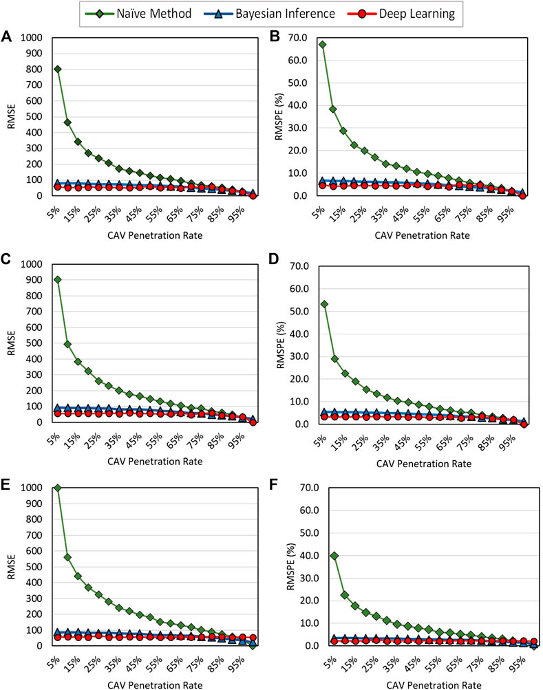
FIGURE 6. RMSE and RMSPE for different traffic demand; (A) RMSE for low demand; (B) RMSPE for low demand; (C) RMSE for medium demand; (D) RMSPE for medium demand; (E) RMSE for high demand; (F) RMSPE for high demand.

Effects of Prior Distribution on Flow Rate Estimation

As presented in Section Overall Results and Findings (with Figure 5), prior information is essential for the Bayesian inference based method. Here, we conduct an additional experiment to examine the effect of prior distribution on the flow rate estimation. Specifically, we consider three different gamma distributions as prior distributions with the same mean of 2,000 veh/hr but different deviations of 200, 500, and 800 veh/hr (referred to as small, medium, and large deviations hereafter). Thus, the [shape, scale] for each Gamma distribution are [100, 20], [16, 125] and [6.25, 320] respectively. Notably, the small deviation represents the case that historical flow rates are similar whereas the large deviation represents a wide variation in historical flow rates. Figure 7 presents RMSEs of flow rate estimation with different prior distributions. Note that the (blue) line with triangular markers is the same as the one in Figure 4D for the Bayesian inference based method. In low penetration (<35%), RMSEs are similar for the cases of small deviation and medium deviation. However, as the penetration rate increases, the RMSE improves more slowly for the small deviation case. Evidently, the prior distribution with the small deviation has greater influence on the flow estimation and actually hinders the estimation when there is sufficient real-time information. One can see in Figure 5 that a narrower prior distribution (with the same mean) would “pull” the posterior distribution closer to the prior distribution. On the other hand, the prior distribution with the large deviation does not provide much information when needed to estimate the flow rate at a low CAV penetration rate, contributing to relatively large RMSE values. However, the accuracy of flow estimation improves quickly as the real-time data becomes more available because the prior distribution has weak influence on the estimation process due to its large deviation. The results suggested that the Bayesian inference based method should be adopted with caution, considering the features of prior information and availability of real-time data (traffic demand, CAV penetration rate).

FIGURE 7

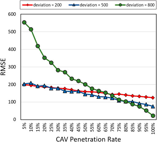
FIGURE 7. RMSE for different deviation of historical data.

Probability Distribution of Flow Rate From Bayesian Inference Based Method

One distinguishing feature of Bayesian inference is that it derives a flow rate distribution rather than a value, unlike the other methods. This means that we can use the mean or mode of the posterior distribution as a specific estimation, but also estimate the probability that the flow rate exceeds a certain value. This is a nice feature as it can be used to quantify the probability of traffic breakdown (Elefteriadou et al., 1995; Persaud et al., 1998; Evans et al., 2001; Brilon et al., 2005; Shiomi et al., 2011; Chen et al., 2014; Han and Ahn, 2018), which can be used for proactive control to prevent traffic breakdown. Thus, this feature is a notable advantage of the Bayesian inference method. For example, we consider a critical flow rate, $q_c$, at 2,200 veh/hr and estimate the probability that the flow rate exceeds $q_c$ at different penetration rates, as presented in Figures 8A–J. The x-axis is the actual flow rate, and the y-axis shows the estimated probability that $\widehat{q}>q_c$. Assuming 0.5 as the critical probability to determine the accuracy of the estimation, the four quadrants (see Figure 8A) represent different categories as: 1Q is “Hit” that $\widehat{q}>q_c$ when $q>q_c$, 2Q is the “False Alarm” that $\widehat{q}>q_c$ when $q<q_c$, 3Q is the “Correct Rejection” that $\widehat{q}<q_c$ when $q<q_c$, and 4Q is the “Miss” hat $\widehat{q}<q_c$ when $q>q_c$. The rates of Hit and False Alarm are shown in Figure 8K. The Hit rate increases with the CAV penetration rate while the False Alarm rate decreases.

FIGURE 8

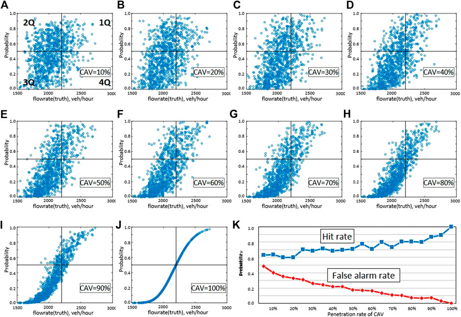
FIGURE 8. (A)–(J) Probability over critical flow rate through Bayesian inference; (K) Hit and False alarm rates.

Validation With Real Data

Data and Assumptions

The proposed methods are validated with real data. We use the NGSIM prototype data (NGSIM, 2006) for a section of I-80 near the San Francisco Bay Area, CA. This freeway section is 3,000 ft long and has six lanes, including a high-occupancy vehicle lane, and the data was collected for a 30 min period in December 2003 at the resolution of 1/15 of a second. Note that the prototype NGSIM data includes both free flow and congested traffic states.

We divide the time-space domain into 450 subsections that are 100 feet by 2 min. From the vehicle trajectories, we derive headway data at the midpoint of each subsection as shown earlier in Figure 1, and calculate the actual flow rate for each subsection using all the headways. Then, we randomly designate “CAVs” considering the penetration rate and estimate a flow rate by each method using the CAV headway data. For the Deep-learning method, 315 subsections (70%) are used for model training, and 67 and 68 subsections (15% each) are used for validation and test, respectively.

For the Bayesian inference method, prior information is required; however, historical data at the NGSIM site is not available. Instead, we investigate the flow rate near the NGSIM site to observe its general characteristics over time. Specifically, we analyzed the data in 2004 through the Performance Measurement System (PeMS, 2018) at a detector location downstream of the NGSIM site⁴. We found that historic flow rates in that area are distributed in a typical bell-shaped curve, but the distribution varies by time of day, as illustrated in Figure 9. This feature was also observed in the NGSIM data: the flow rate was similar throughout the site around the same time, but it changed over time as expected. Based on this observation, we assume that each time step (2 min in this evaluation) has a prior distribution following a gamma distribution with a mean of the average flow rate (over all locations) at that time step in the NGSIM data. The deviation of the prior distribution is assumed relatively large at 500 veh/hr to avoid the correlation between the data and the estimated prior distribution. Note that we obtained 15 prior distributions for the study duration, and each prior distribution applies to all locations. The likelihood function is used as exponential distribution as the most state is free flow state with random vehicle arrivals.

FIGURE 9

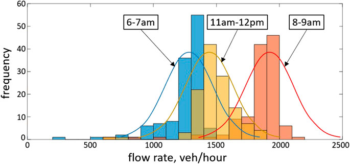
FIGURE 9. Example of distribution of historical flow rates (Detector # = 400679 on I-80, CA, July-Dec, 2004).

Validation Results

Figure 10 presents an example of the flow rate estimation results by each method with different CAV penetration rates. Similar to the numerical experiment, the naïve method shows scattered results at a low penetration rate and a large value of RMSE, but the points gradually move to the reference line with smaller RMSE as the penetration rate increases. On the other hand, the Bayesian inference method estimates well even at low penetration rates, and the RMSE steadily decreases with increasing penetration rates. This could be due to the potentially close relationship between the actual flow rates and the assumed prior distributions. Thus, to apply the Bayesian inference, the prior information should represent a general traffic state of the target site. When the traffic condition changes significantly (e.g., a sudden demand increase), the prior distribution should be redefined. Lastly, the deep learning method shows better performance particularly at a low penetration rate. Notably, compared to the multiple linear regression, the deep learning based method clearly performs better with real data, demonstrating that the deep learning based method can better describe the relationship between the CAV headway and the flow rate.

FIGURE 10

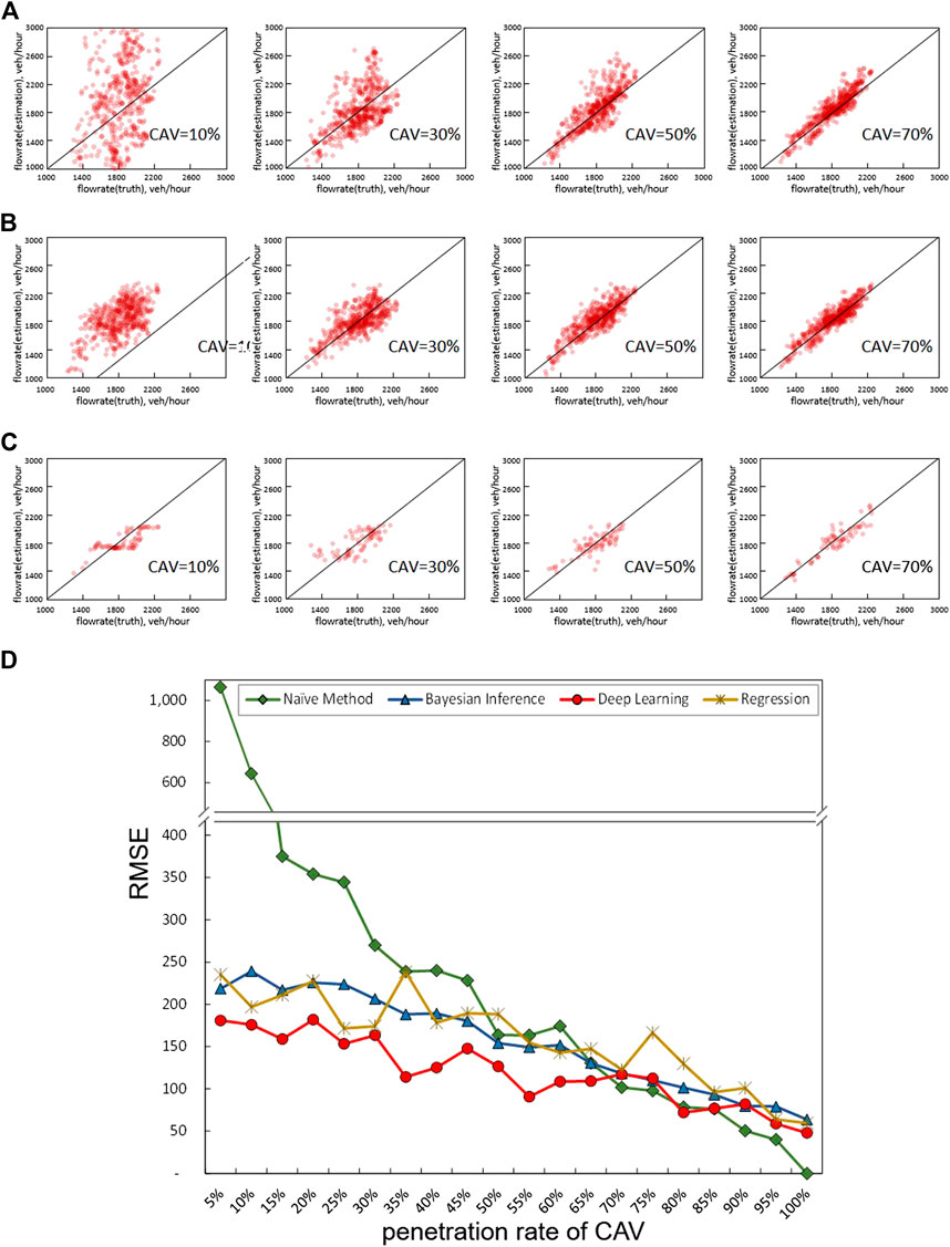
FIGURE 10. Example of validation with NGSIM data (Lane 2, I-80) with different CAV penetration rate: (A) Naïve method; (B) Bayesian inference; (C) Deep learning; (D) RMSE by penetration rate of CAV for each method.

Conclusion and Discussion

This paper presented flow rate estimation methods using headway data that can presumably be collected from CAVs. Specifically, we developed Bayesian inference and deep learning based methods and evaluated their performance against a baseline, naïve method based on the simple arithmetic mean of headways. The proposed methods were investigated by numerical experiments and validated with real data. The results show that the Bayesian inference based method can be an effective algorithm to estimate flow rate distribution by integrating current (real-time) data and previous knowledge, such as historical data. It shows good performance (in terms of accuracy and precision) with a proper prior distribution and a likelihood function even at low penetration rates (<20%). Thus, this method can be used when historical traffic information, consistent with the current traffic condition, is readily available. However, as the CAV penetration or demand increases, its relative advantage to the other methods (the deep learning based method and even the simple average) wanes because the prior information always influences the flow rate estimation. Particularly, in high CAV penetration, where real-time CAV information alone suffices for accurate flow estimation, inclusion of prior information can actually hinder the accuracy. The deep learning based method is found to perform reasonably well using only CAV data when the CAV penetration rate is moderate to high (>20%). Particularly it shows superior performance in characterizing the complicated relationship in the real world than other methods considered in this study. However, when the data is sparse (in light traffic, low CAV penetration, or a small number of data), the method produces an estimate close to the mean of the training data regardless of real-time observations. Finally, at a relatively high CAV penetration rate (>70%), the relative advantage of the advanced methods is negligible and in fact, the naïve method is preferred in terms of accuracy as well as efficiency.

To improve the proposed methods, we suggest several future research directions. For the Bayesian inference based method, we mainly used the exponential-gamma conjugate system for the prior distribution and likelihood function for analytical tractability. Though these assumptions are reasonable to address general characteristics of free-flow traffic, more site-specific functions with calibration would be necessary to apply in practice. Furthermore, probabilistic distributions of CAVs should be considered to facilitate theoretical analysis.

For the deep learning based method, we have adopted this approach to better capture the complicated relationship between sampled headways and flow rate in free-flow traffic due to randomness in vehicle arrivals. Though the deep learning based method shows better performance than the other methods considered, particularly in real world estimation, it still has significant error in low CAV penetration. Its performance may improve if other factors, such as time of day, weather, historical traffic information, are considered as input features. In addition, due to the limitation of NGSIM data, the proposed deep learning based method is validated with a small dataset, which limits the applicability of this method. An improvement of this method may be possible with a larger dataset and a deeper architecture. Notably the proposed deep learning approach shows better performance than the naïve method even though both methods use the same input data. However, considering other available data, advanced algorithms such as LSTM or Convolutional neural network should be considered to reveal hidden features in a larger dataset. In addition, this paper assumed that CAVs’ behavior is similar to the behavior of human-driven vehicles in a free flow state; however, CAVs’ behavior may be altered significantly in some situations due to advanced CAV operations (e.g., platooning, exclusive lane policy). Alternative methods should be developed in such cases. Finally, for the validation with real data, we used all observed data from the NGSIM vehicle trajectory data, some of which may be influenced by merging or lane-changing. Systematic data filtering is desirable in the future to further improve the model performance. Nonetheless, this study presents some insight into how advanced methods can be adopted to address challenges such as the one explored in this study and provides a building block for future studies.

Data Availability Statement

Publicly available datasets were analyzed in this study. This data can be found here: ITS DataHub [https://its.dot.gov/data/] and Caltrans Performance Measurement System (PeMS) [pems.dot.ca.gov].

Author Contributions

YH: conceptualization, literature review, methodology, numerical experiment, validation, results analysis, results visualization, and manuscript-draft. SA: results analysis, manuscript-revision, and supervision.

Funding

The authors gratefully acknowledge the National Science Foundation for sponsoring this research through Award CMMI 1536599.

Conflict of Interest

The authors declare that the research was conducted in the absence of any commercial or financial relationships that could be construed as a potential conflict of interest.

Footnotes

¹CAV might measure the spacing of following vehicle as well. However, in this paper, we only consider data related leading vehicle since the detected rear range is typically shorter than front range. If the behind data is available, however, proposed method can be operated with more data, and the framework and features of proposed methods are same.

²Density can be derived using spacing data of CAV through the same framework in following sections. But, for the Bayesian inference (in Bayesian Inference), enough prior knowledge and likelihood function of spacing for given density would be required.

³We also conducted the same experiment with 3,000 data set splitting into three groups of training, validation, and testing with 1,000 data set for each. The results are similar in terms of accuracy (in RMSE) and trends in the scatter plot.

⁴The NGSIM prototype data was collected in December 2003. However, the quality of the PeMS data near the NGSIM site in 2003 was not desirable according to their data quality assessment. Therefore, we used the data in 2004 instead.

References

Beale, M. H., Hagan, M. T., and Demuth, H. B. (2015). Neural network toolbox user’ s guide. Boston, MA: PWS.

Bekiaris-Liberis, N., Roncoli, C., and Papageorgiou, M. (2017). Highway traffic state estimation per lane in the presence of connected vehicles. Transportation Res. B: Methodological 106, 1–28. doi:10.1016/j.trb.2017.11.001

CrossRef Full Text | Google Scholar

Bekiaris-Liberis, N., Roncoli, C., and Papageorgiou, M. (2016). Highway traffic state estimation with mixed connected and conventional vehicles. IEEE Trans. Intell. Transport. Syst. 17, 3484–3497. doi:10.1109/TITS.2016.2552639

CrossRef Full Text | Google Scholar

Brilon, W., Geistefeldt, J., and Regler, M. (2005). “Reliability of freeway traffic flow,” in Proceedings 16th international symposium transportation and traffic theory, College Park, MA, July 19–21, 2005, 125–144. doi:10.1016/b978-008044680-6/50009-x

CrossRef Full Text | Google Scholar

Chen, X., Li, Z., Li, L., and Shi, Q. (2014). A traffic breakdown model based on queueing theory. Netw. Spat. Econ. 14, 485–504. doi:10.1007/s11067-014-9246-6

CrossRef Full Text | Google Scholar

Edie, L. (1963). “Discussion of traffic stream measurements and definitions,” in Proceedings of the second international symposium on the theory of traffic flow, London, June 1963, 139–154.

Google Scholar

Elefteriadou, L., Roess, R. P., and McShane, W. R. (1995). Probabilistic nature of breakdown at freeway merge junctions. Transp. Res. Rec. 1484, 80–89 .

Google Scholar

Elfar, A., Xavier, C., Talebpour, A., and Mahmassani, H. S. (2018). Traffic shockwave detection in a connected environment using the speed distribution of individual vehicles. Transportation Res. Rec. 2672, 203–214. doi:10.1177/0361198118794717

CrossRef Full Text | Google Scholar

Evans, J. L., Elefteriadou, L., and Gautam, N. (2001). Probability of breakdown at freeway merges using Markov chains. Transportation Res. Part B: Methodological 35, 237–254. doi:10.1016/S0191-2615(99)00049-1

CrossRef Full Text | Google Scholar

Fei, X., Lu, C.-C., and Liu, K. (2011). A bayesian dynamic linear model approach for real-time short-term freeway travel time prediction. Transportation Res. C: Emerging Tech. 19, 1306–1318. doi:10.1016/j.trc.2010.10.005

CrossRef Full Text | Google Scholar

Fountoulakis, M., Bekiaris-Liberis, N., Roncoli, C., Papamichail, I., and Papageorgiou, M. (2017). Highway traffic state estimation with mixed connected and conventional vehicles: microscopic simulation-based testing. Transportation Res. Part C: Emerging Tech. 78, 13–33. doi:10.1016/j.trc.2017.02.015

CrossRef Full Text | Google Scholar

Fusco, G., Colombaroni, C., and Isaenko, N. (2016). Short-term speed predictions exploiting big data on large urban road networks. Transportation Res. Part C: Emerging Tech. 73, 183–201. doi:10.1016/j.trc.2016.10.019

CrossRef Full Text | Google Scholar

Han, Y., and Ahn, S. (2018). Stochastic modeling of breakdown at freeway merge bottleneck and traffic control method using connected automated vehicle. Transportation Res. Part B: Methodological 107, 146–166. doi:10.1016/j.trb.2017.11.007

CrossRef Full Text | Google Scholar

Han, Y., Chen, D., and Ahn, S. (2017). Variable speed limit control at fixed freeway bottlenecks using connected vehicles. Transportation Res. Part B: Methodological 98, 113–134. doi:10.1016/j.trb.2016.12.013

CrossRef Full Text | Google Scholar

Hegyi, A., Netten, B. D., Wang, M., Schakel, W., Schreiter, T., Yuan, Y., et al. (2013). “A cooperative system based variable speed limit control algorithm against jam waves—an extension of the SPECIALIST algorithm,” in 16th International IEEE Conference on Intelligent Transportation Systems, Hague, Netherlands, October 6–9, 2013, 2, 973–978. doi:10.1109/ITSC.2013.6728358

CrossRef Full Text | Google Scholar

Hofleitner, A., Herring, R., Abbeel, P., and Bayen, A. (2012). Learning the dynamics of arterial traffic from probe data using a dynamic bayesian network. IEEE Trans. Intell. Transport. Syst. 13, 1679–1693. doi:10.1109/TITS.2012.2200474

CrossRef Full Text | Google Scholar

Jintanakul, K., Chu, L., and Jayakrishnan, R. (2009). Bayesian mixture model for estimating freeway travel time distributions from small probe samples from multiple days. Transportation Res. Rec. 2136, 37–44. doi:10.3141/2136-05

CrossRef Full Text | Google Scholar

Julio, N., Giesen, R., and Lizana, P. (2016). Real-time prediction of bus travel speeds using traffic shockwaves and machine learning algorithms. Res. Transportation Econ. 59, 250–257. doi:10.1016/j.retrec.2016.07.019

CrossRef Full Text | Google Scholar

Jun, H. J., Park, J. K., and Bae, C. H. (2017). “Deep leaning neural networks for determining replacement timing of steel water transmission pipes,” in International conference on control, artificial intelligence, robotics and optimization (ICCAIRO), Prague, Czech Republic, May 20–22, 2017 (IEEE), 219–225.

Google Scholar

Khodayari, A., Ghaffari, A., Kazemi, R., and Braunstingl, R. (2012). A modified car-following model based on a neural network model of the human driver effects. IEEE Trans. Syst. Man. Cybern. A. 42, 1440–1449. doi:10.1109/TSMCA.2012.2192262

CrossRef Full Text | Google Scholar

Kim, J., and Wang, G. (2016). Diagnosis and prediction of traffic congestion on urban road networks using bayesian networks. Transportation Res. Rec. 2595, 108–118. doi:10.3141/2595-12

CrossRef Full Text | Google Scholar

Lefevre, S., Carvalho, A., and Borrelli, F. (2016). A Learning-based framework for velocity control in autonomous driving. IEEE Trans. Automat. Sci. Eng. 13, 32–42. doi:10.1109/TASE.2015.2498192

CrossRef Full Text | Google Scholar

Li, L., and Chen, X. M (2017). Vehicle headway modeling and its inferences in macroscopic/microscopic traffic flow theory: a survey. Transportation Res. Part C: Emerging Tech. 76, 170–188. doi:10.1016/j.trc.2017.01.007

CrossRef Full Text | Google Scholar

Ma, X., Tao, Z., Wang, Y., Yu, H., and Wang, Y. (2015). Long short-term memory neural network for traffic speed prediction using remote microwave sensor data. Transportation Res. Part C: Emerging Tech. 54, 187–197. doi:10.1016/j.trc.2015.03.014

CrossRef Full Text | Google Scholar

Mathew, T. V., and Ravishankar, K. V. R. (2012). Neural network based vehicle-following model for mixed traffic conditions. Eur. Transport 52 (4), 1–15.

Google Scholar

Motamedidehkordi, N., Amini, S., Hoffmann, S., Busch, F., and Fitriyanti, M. R. (2017). “Modeling tactical lane-change behavior for automated vehicles: a supervised machine learning approach,” in 5th IEEE International conference on models and technologies for intelligent transportation systems, Naples, Italy, June, 2017 (IEEE), 268–273. doi:10.1109/MTITS.2017.8005678

CrossRef Full Text | Google Scholar

Neumann, T., Bohnke, P. L., and Touko Tcheumadjeu, L. C. (2013). “Dynamic representation of the fundamental diagram via Bayesian networks for estimating traffic flows from probe vehicle data,” in 16th IEEE conference.on intelligent transportation system ITSC. Hague, Netherlands, October 6–9, 2013. doi:10.1109/ITSC.2013.6728501

CrossRef Full Text | Google Scholar

NGSIM (2006). Next generation simulation. Available at: https://ops.fhwa.dot.gov/trafficanalysistools/ngsim.htm (Accessed September 10, 2002).

Google Scholar

Ozguven, E. E., and Ozbay, K. (2008). Nonparametric bayesian estimation of freeway capacity distribution from censored observations. Transportation Res. Rec. 2061, 20–29. doi:10.3141/2061-03

CrossRef Full Text | Google Scholar

Papadopoulou, S., Roncoli, C., Bekiaris-Liberis, N., Papamichail, I., and Papageorgiou, M. (2018). Microscopic simulation-based validation of a per-lane traffic state estimation scheme for highways with connected vehicles. Transportation Res. Part C: Emerging Tech. 86, 441–452. doi:10.1016/j.trc.2017.11.012

CrossRef Full Text | Google Scholar

Papathanasopoulou, V., and Antoniou, C. (2015). Towards data-driven car-following models. Transportation Res. Part C: Emerging Tech. 55, 496–509. doi:10.1016/j.trc.2015.02.016

CrossRef Full Text | Google Scholar

PeMS (2018). Freeway performance measurement system. Available at: http://pems.dot.ca.gov/ (Accessed July 7, 2018).

Google Scholar

Persaud, B., Yagar, S., and Brownlee, R. (1998). Exploration of the breakdown phenomenon in freeway traffic. Transportation Res. Rec. 1634, 64–69. doi:10.3141/1634-08

CrossRef Full Text | Google Scholar

Piotrowski, A. P., and Napiorkowski, J. J. (2013). A comparison of methods to avoid overfitting in neural networks training in the case of catchment runoff modelling. J. Hydrol. 476, 97–111. doi:10.1016/j.jhydrol.2012.10.019

CrossRef Full Text | Google Scholar

Polson, N. G., and Sokolov, V. O. (2017). Deep learning for short-term traffic flow prediction. Transportation Res. Part C: Emerging Tech. 79, 1–17. doi:10.1016/j.trc.2017.02.024

CrossRef Full Text | Google Scholar

Roncoli, C., Papageorgiou, M., and Papamichail, I. (2015). Motorway traffic flow optimisation in presence of vehicle automation and communication systems. Comput. Methods Appl. Sci. 38, 1–16. doi:10.1007/978-3-319-18320-6_1

CrossRef Full Text | Google Scholar

Rumelhart, D. E., Hinton, G. E., and Williams, R. J. (1986). Learning representations by back-propagating errors. Nature 323, 533–536. doi:10.1038/323533a0

CrossRef Full Text | Google Scholar

Seo, T., Bayen, A. M., Kusakabe, T., and Asakura, Y. (2017). Traffic state estimation on highway: a comprehensive survey. Annu. Rev. Control 43, 128–151. doi:10.1016/j.arcontrol.2017.03.005

CrossRef Full Text | Google Scholar

Seo, T., Kusakabe, T., and Asakura, Y. (2015). Estimation of flow and density using probe vehicles with spacing measurement equipment. Transportation Res. Part C: Emerging Tech. 53, 134–150. doi:10.1016/j.trc.2015.01.033

CrossRef Full Text | Google Scholar

Seo, T., and Kusakabe, T. (2015). Probe vehicle-based traffic state estimation method with spacing information and conservation law. Transportation Res. Part C: Emerging Tech. 59, 391–403. doi:10.1016/j.trc.2015.05.019

CrossRef Full Text | Google Scholar

Shiomi, Y., Yoshii, T., and Kitamura, R. (2011). Platoon-based traffic flow model for estimating breakdown probability at single-lane expressway bottlenecks. Transportation Res. Part B: Methodological 45, 1314–1330. doi:10.1016/j.trb.2011.05.008

CrossRef Full Text | Google Scholar

Simonelli, F., Bifulco, G. N., Martinis, V. D., and Punzo, V. (2015). “Human-like adaptive cruise control systems through a learning machine approach,” in Applications of soft computing, 240–249. doi:10.1016/j.limno.2013.04.005

CrossRef Full Text | Google Scholar

Wei, J., Dolan, J. M., and Litkouhi, B. (2010). “A learning-based autonomous driver: emulate human driver’s intelligence in low-speed car following,” in The International Society for Optical Engineering, Orlando, FL, April 5–9, 2010 (IEEE), 76930L. doi:10.1117/12.852413

CrossRef Full Text | Google Scholar

Zheng, J., Suzuki, K., and Fujita, M. (2013). Car-following behavior with instantaneous driver-vehicle reaction delay: a neural-network-based methodology. Transportation Res. Part C: Emerging Tech. 36, 339–351. doi:10.1016/j.trc.2013.09.010

CrossRef Full Text | Google Scholar

Zhou, M., Qu, X., and Li, X. (2017). A recurrent neural network based microscopic car following model to predict traffic oscillation. Transportation Res. Part C: Emerging Tech. 84, 245–264. doi:10.1016/j.trc.2017.08.027

CrossRef Full Text | Google Scholar