Quantifying and mitigating bias and increased variability when using large-scale estimates of forests for subdomains

This paper presents an empirical method to calculate a conservative discount factor when applying a large-scale estimate to an internal subset of areas (subdomains) that accounts for both the precision (variability) and potential bias of the estimate of the subset (i.e., the small area estimated within the large-scale framework). This method is presented in the context of forest carbon offset quantification and therefore considers how to conservatively adjust a large-scale estimate when applied to a subdomain within the original estimation domain. The approach outlined can be used for individual or aggregated carbon projects and allows large-scale estimates of forest stocks to be scaled down to project and stand-level results by discounting estimates to account for the potential variability and bias of the estimates. The conceptual basis for this approach is built upon a method described in Neeff’s 2021 publication and in 2024 was adopted by the American Carbon Registry for use in the Small Non-Industrial Private Forestlands (SNIPF) methodology. Although this publication uses an example dataset from the Southeastern United States and is specific to the ACR SNIPF Improved Forest Management (IFM) protocol, the intent of this study is to introduce a method that can be applied in any forest type or geography using any forest carbon offset protocol where there exist independent estimates of forest carbon stocks that overlap with the large-scale estimates. The application of this method relies on user-defined levels of risk and inventory confidence combined with the distribution of observed error. This method allows remote sensing estimates of carbon stocks to be applied to forest carbon offset quantification. By doing so, this approach can reduce the costs for forest landowners and can therefore help to increase the impact of these market-based forest carbon offset programs on forest conservation and climate change mitigation.

1 Introduction

Quantifying forest attributes at large scales has been a topic of scientific research and commercial importance for over 40 years (Justice et al., 1985; Running et al., 1995; Turner et al., 2006; Wilson et al., 2013; Cohen et al., 2017; Bell et al., 2022). Applying large-scale estimates to smaller subdomains within the original estimate can result in reduced accuracy (bias) and a loss of precision (increased variability) (Rao and Molina, 2015). This presents a major obstacle to using large-scale estimation (either model- or design-based approaches) in the context of forest carbon quantification and climate change mitigation. There have been many recent efforts to use small area estimation (SAE) techniques to improve forest attribute estimation and efficiency (Breidenbach and Astrup, 2012; Ståhl et al., 2016; Green et al., 2020; Coulston et al., 2021; Cao et al., 2022; Dettmann et al., 2022; Frescino et al., 2022). However, even SAE requires some inventory data to calibrate and constrain model estimates. Furthermore, the potential bias and increased variability of subdomain estimates using an SAE framework without inventory data remains unknown.

This paper presents an empirical method to calculate a conservative discount factor for a large-scale estimate to an internal subset of areas (subdomains) that accounts for both the precision (variability) and potential bias of the estimate of the subset (i.e., the small area estimated within the large-scale framework). This method is presented in the context of forest carbon offset quantification and therefore considers how to conservatively adjust a large-scale estimate when applied to a subdomain within the original estimation domain. The approach outlined can be used for individual or aggregated carbon projects and allows large-scale estimates of forest stocks to be scaled down to project and stand-level results by discounting estimates to account for the potential variability and bias of the estimates.

The conceptual basis for this approach is built upon a method described in Neeff (2021) and has been adopted (American Carbon Registry, 2021a) by the American Carbon Registry for use in the Small Non-Industrial Private Forestlands (American Carbon Registry, 2021b) (SNIPF). Although this publication uses an example dataset from the Southeastern United States and is specific to the ACR SNIPF IFM protocol, the approach described here can be applied in any forest type or geography using any forest carbon offset protocol where there exist independent estimates of forest carbon stocks that overlap with the large-scale estimates. The reason for this is that this method is based solely on the distribution of errors observed between a large-scale estimate and subdomains paired with concepts of statistical risk and confidence. For example, large-scale estimates of tropical forests when compared to subdomain observations will generate the same sorts of conclusions irrespective of the unique attributes of that specific forest ecosystem.

1.1 Climate change and forest loss

Forest carbon offsets are a critical tool to mitigate climate change and protect the myriad co-benefits offered by forests. Climate change combined with increasing global forest loss and degradation presents two of the greatest challenges to the functioning of ecosystems and the continued health of this planet (Core Writing Team, 2023). Globally, deforestation continues to be a driver of land use carbon emissions (Hansen et al., 2013; Curtis et al., 2018; Bullock et al., 2020), (McNulty et al., 2015; Fitts et al., 2021; Nedd and Anandhi, 2022). Current climate change mitigation policies and commitments leave a substantial gap that needs to be filled to meet stated atmospheric CO₂ goals (Shukla et al., 2022).

1.2 Forest carbon offsets

To address the dual threats of increasing global CO₂ emissions and increasing forest loss and degradation, forest carbon offset protocols have been developed to provide methodologies to account for the emission reductions and removals generated by protecting forests (American Carbon Registry, 2021b; Architecture for REDD+ Transactions, 2021; American Carbon Registry, 2023b; Climate Action Reserve, 2023; Verra, 2023). In some jurisdictions, methodologies have been approved by legislative bodies and adopted to allow businesses covered by carbon taxes or carbon caps to use offsets generated by forests to reduce their costs of complying with CO₂ emissions reduction policies (Núñez and Pavley, 2006; Compliance Offset Protocol US Forest Projects, 2015; Order of the Minister of the Environment, the Fight Against Climate Change, Wildlife and Parks dated 17 November 2022, 2021; RCW 70A.45.020: Greenhouse gas emissions reductions—Reporting requirements, 2023).

Forest carbon offsets can be generated in several distinct ways. The general frameworks for carbon offset projects occur at a project level or a jurisdictional level. Jurisdictional-level carbon projects occur across countries or large regions and attempt to measure and quantify the changes in forest carbon stocks based on large-scale estimates of baselines and activities (von Essen and Lambin, 2021). Project-level carbon projects occur at the landowner scale and typically reflect the individual’s rather than the government’s agreement to abide by the principles and rules defined in forest carbon standards.

When estimating the carbon stored in forests for the purposes of carbon offsets, there are many sources of uncertainty. These range from the uncertainty inherent in any sample, the uncertainty in any modeled projections of forest growth or forest management (i.e., growth and yield model uncertainty), and the uncertainty in the allometric equations used to convert tree measurements to volume, biomass, and carbon. Most standards ignore allometric model and growth and yield model uncertainty (though there have been proposals to include and propagate these sources of uncertainty; Holdaway et al., 2014; Vorster et al., 2020; Lin et al., 2023).

Despite these myriad sources of uncertainty, carbon offset protocols require calculating a single number to represent the climate impact that a given project has on the climate. As a result, these protocols require conservative discount factors to be calculated to ensure that any claimed climate benefits can be conservatively estimated (Architecture for REDD+ Transactions, 2021; Verra, 2023).

There are many different types of forest carbon offsets, but all generally apply similar principles to ensure the integrity of the offsets generated (Climate Action Reserve, 2019; American Carbon Registry, 2023a; The Integrity Council for the Voluntary Carbon Market, 2024). One of the consistent themes through all types of forest carbon offset programs and all sets of principles is the need to accurately and precisely quantify the actual carbon stocks and CO₂ removals and reductions claimed by a given project. The discounting of the claimed offsets is crucial when considering that offsets used by emitters are considered equivalent to emissions to balance businesses’ carbon budgets. With this context in mind, we propose a method to conservatively discount estimate(s) of a claimed climate benefit (i.e., tons of CO₂ removed from or avoided from being emitted to the atmosphere) due to engaging in a forest carbon offset project. The method outlined in this publication has been adopted by the American Carbon Registry for their Small Non-Industrial Private Forestlands methodology (American Carbon Registry, 2021b).

1.3 Forest carbon estimation methods

Accurate and precise estimates of forest carbon stocks are the foundation upon which all quantification of carbon offsets is built. The specifics of some of the overarching estimation approaches are detailed below to provide some context for how large-scale estimates are built. However, the distinctions (Gregoire, 1998; Sterba, 2009) between these methods are less important than the overarching similarity of the potential bias and increased variability that is introduced when applying a large-scale estimate to an internal subdomain.

1.3.1 Design-based estimation

Design-based (DB) estimation does not assume or require any underlying structure of the sampled population. Instead, it uses a probability sample where the probability of each sample unit’s inclusion is known. There are many ways to improve the efficiency of design-based estimation that impose more structure on the underlying data (e.g., stratification and post-stratification) or use auxiliary variables to correct sample estimates (model-assisted estimation) (Gregoire et al., 2011; Næsset et al., 2011; Ståhl et al., 2016; McConville et al., 2017; McConville et al., 2020; Wojcik et al., 2022). These DB approaches are asymptotically design-unbiased. All these techniques require that samples be available in any location where an estimate is produced.

1.3.1.1 Model-assisted estimation

A more complicated and potentially more powerful subset of design-based estimation is model-assisted (MA) estimation. This type of estimation framework is introduced here to more fully describe the space of design-based approaches. Counter-intuitively, model-assisted estimation is a design-based approach that includes modeled components.

MA methods are asymptotically design-unbiased. These methods make estimates based on models that relate auxiliary data to sample data from a probability sample. In their simplest forms, ratio and regression estimators are MA estimators. MA methods have often been used to estimate values in small areas. However, their design-unbiasedness is only asymptotic and does not hold when small areas have minimal sample sizes (< 5 samples) (Næsset et al., 2011). MA methods are not considered models that generate the population of possible values in a given location, but rather they assist in partitioning the variability of the probability design-based sample (Corona et al., 2014). MA estimates are powerful tools for estimating quantities in small areas and are often compared to design-based and composite estimators (Ståhl et al., 2016; Guldin, 2021). The equation below is a typical MA form (taken from Ståhl et al., 2016):

$\begin{array}{ll}{\widehat{\tau }}_{MA}={\displaystyle \sum _{i\in U}}{\widehat{y}}_i+{\displaystyle \sum _{i\in s}}\frac{\left(y_i-{\widehat{y}}_i\right)}{{\pi }_i}& (1)\end{array}$

In Equation 1, ${\widehat{y}}_i$ is the prediction generated by a model fitted to predictor variables for each ith observation. The second summand shows that the model-based (MB) predictions in the first summand are scaled by the difference between the observed and predicted values (as Stahl explains “this is the Horvitz-Thompson estimator of the total of deviations between observed $y_i$ and predicted values” scaled by the probability of inclusion of each observation (${\pi }_i$)). This scaling (difference estimator) causes MA estimators to be unbiased for larger sample sizes. Said another way, MA estimators correct their predictions based on the prediction error relative to the observed values from the design-based sample (see equation above).

1.3.2 Model-based estimation

Model-based (MB) inference develops relationships between predictor variables and response variables to estimate finite population parameters. These models often have low variance but may have a significant bias as they are only constrained by the data they are trained on. If assumptions are violated when they are constructed, or the input data are not representative of the feature modeled, there are no guarantees or supports that prevent a model-based estimate from exhibiting large bias in small areas. That said, large-scale model-based estimates of forest parameters have been shown to be strong predictors of forest attributes at smaller scales (McRoberts et al., 2019).

1.3.2.1 Small area (composite) estimation

Small area estimation (SAE) is a statistical estimation method designed to combine model-based or synthetic estimates with design-based estimates. As a result, SAE approaches are often called “composite estimators.” These composite estimators can take on many forms, but a fundamental feature of this approach is that the final estimate generated is a weighted combination of the design-based and model-based estimates of the parameter of interest. The weighting is based on the variance of the design-based estimate. The larger the variance, the more weight is given to the model-based estimator. The smaller the variance of the design-based estimate (hence the more precise), the more weight is given to the design-based estimator (Magnussen et al., 2017).

Using an SAE framework has been shown to create more precise and statistically unbiased estimates of finite population forest parameters (Rao and Molina, 2015; Guldin, 2021; Dettmann et al., 2022). However, applying this approach in locations where subdomains may have little or no direct samples is difficult, as the design-based variance estimates in these locations may be very large or non-existent. Because SAE uses model-based results, it is best considered a subset of model-based estimation. However, unlike a purely model-based approach, SAE constrains the model-based estimates based on the design-based estimator’s variance, protecting against large biases that purely model-based estimators might introduce (but only in cases where inventory data exist) (see Equation 2).

Equation 2 below is a typical formulation of the scaling or shrinkage factor that is used to weight model-based estimates by the sample variability of the target unit or area (taken from Dettmann et al., 2022). ${\widehat{\tau }}_d^{\mathit{\text{COMP}}}$ is the composite or small area estimator for a given domain d. ${\gamma }_d$ is the shrinkage factor that is between 0 and 1 and is based on the variability of the direct sample in that domain. The DIR superscript refers to the direct sample-based estimate and the SYN superscript refers to the synthetic model-based estimate for each domain d.

$\begin{array}{ll}{\widehat{\tau }}_d^{\mathit{\text{COMP}}}={\gamma }_d{\widehat{\tau }}_d^{DIR}+\left(1-{\gamma }_d\right){\widehat{\tau }}_d^{SYN}& (2)\end{array}$

Most literature examining SAE methods is focused on reducing the variance of estimators relative to design-based samples as opposed to evaluating the bias of the estimates (with few exceptions; Katila, 2006; Goerndt et al., 2013; Wojcik et al., 2022). Applying SAE methods is an effective way to leverage the power of design-based samples and model-based approaches even in cases where the small area matches the extent of the original survey. That is, the power of the SAE method extends beyond situations where estimates are needed for small areas but can also be used to combine estimation approaches for large areas as well (Saarela et al., 2015a; Saarela et al., 2015b; Saarela et al., 2016; Babcock et al., 2018).

1.4 Subdomain (small area) relative bias

The problem of estimating subdomain (SD) bias and increased variability occurs in any situation where an estimator and the associated uncertainty of the estimate are calculated (using either a design- or model-based approach) at a given scale, and then, this large-scale estimate is the basis of a claim for a subdomain of this large-scale estimate (this is complicated in cases of design-unbiased model-assisted or composite estimators. In these cases, the specific subdomain, while design-unbiased, may still have a bias). As an example, one may develop a model- or design-based estimate of carbon stocks for a full state in the USA. The estimate at the state level has an associated uncertainty based on the method used typically based on the underlying data used to generate the estimate (e.g., the US Forest Service Forest Inventory and Analysis plot inventory data—described below) as well as the form of the estimate. If this state-level estimate is then applied to a subset of regions (e.g., counties, ownerships, and stands) within the state, there is the potential for this estimate to be biased and have increased variability relative to the state-level estimate.

Regardless of the method used to estimate forest attributes at large scales (e.g., design-based, model-based, and composite), attempting to estimate smaller area subsets or individual unit subsets within the extent of the initial large-scale estimate results in additional estimate uncertainty. In addition, these scenarios add the potential for a bias in the smaller estimate especially when no sample data are available in the small area subset. To understand why this is, it is helpful to consider a 1:1 plot of observed vs. predicted outcomes for small areas or individual units that may be estimated using a model- or design-based approach developed for a larger area.

Figure 1 shows an example 1:1 plot for a given inferential paradigm where the x-axis is the observed values at a given location and the y-axis is the predicted value at that location. The observed values may be individual plots where the predicted values are strata averages calculated by stratified random sampling—a design-based inferential paradigm. Alternatively, the observed values could be individual plots used to train a linear regression model that is then used to predict those values—a model-based paradigm, or any of the other more sophisticated model-assisted or composite/SAE model-based approaches. The ovals labeled a and b show potential subsets of the initial full dataset that might be predicted. In oval b, the selection zone is centered around the 1:1 line, so little bias would be expected in the outcome. Oval a shows a scenario where more bias would be introduced due to the properties of the sub-sample. It is important to consider that the subset of data predicted may not be represented by the original modeled data and may be found outside of the range of variability shown by the observed points. This is possible as some subdomains will not have samples within them.

Figure 1

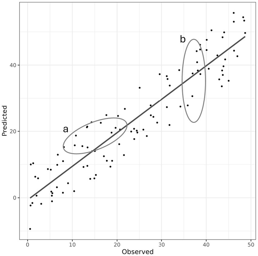
Figure 1. Example subdomains within a large-scale estimate of forest attributes. The diagonal line represents a large-scale model based on the samples (dots). Ellipse b is an unbiased subdomain—the mean of predictions in this domain will be close to the mean of observations. Ellipse a is a biased subdomain—the mean of the predictions in this domain will show a systematic bias relative to the mean of the observations.

In both model- and design-based approaches, it is assumed that individual predictions will have some error based on the underlying variability in the process described by the model or probability sample. The sub-sample of individuals or areas the estimation approach is applied to is assumed to be within the same domain as the original large-scale framework, so inherits the same underlying variability found in the large-scale estimate. However, the subdomain may have a different (larger or smaller) range of variability when compared to the domain used to build the large-scale estimate. This difference could result in a subdomain estimate that exhibits a bias relative to the large-scale estimate.

The question that motivates this research is as follows: how can we estimate the potential bias that may occur within a subdomain of a large-scale inferential framework? Furthermore, is it possible to conservatively correct the potential bias and increased variability of the subdomain using a risk-based framework to calculate a discount factor? The goal of this study is to adjust claimed climate benefits to reduce the risk of over-crediting using this information.

2 Methods

Mitigating potential bias requires estimating the size of the bias and the variability of the potential bias. Below, after defining how bias is calculated, several methods and data sources are introduced to quantify the potential size and variability of subdomain bias. In addition, because over-crediting is the primary concern in the context of carbon offset project development, a method will be introduced to protect against potential bias that inflates estimates of forest carbon stocks by applying a discount factor.

2.1 Relative bias

The first step toward calculating the potential bias that may result for estimates in a subdomain within a broader model is to define the metric that will be used to track this bias. In our case, we will use the relative bias metric for each subdomain i [defined in several publications but taken from Goerndt et al., 2011, 2013 and Wojcik et al., 2022] and shown Equation 3 below:

$\begin{array}{ll}R{B}_i=\left(\frac{{\widehat{Y}}_{iP}-{\widehat{Y}}_{\mathit{\text{iO}}}}{{\widehat{Y}}_{\mathit{\text{iO}}}}\right)\ast 100& (3)\end{array}$

where ${\widehat{Y}}_{iP}$ is the predicted mean estimate for subdomain I, and ${\widehat{Y}}_{\mathit{\text{iO}}}$ is the directly measured sample estimate of subdomain i (and is assumed to be an unbiased estimate of this subdomain). For this study, the ${\widehat{Y}}_{iP}$ prediction may come from any number of estimation approaches (e.g., model-based estimates and design-based estimates). The critical distinction being made here is that this prediction is based on an estimation frame that is larger than the directly measured estimate ${\widehat{Y}}_{\mathit{\text{iO}}}$ that is based only on samples within subdomain i (although ${\widehat{Y}}_{iP}$ may or may not include direct samples in subdomain i, there will be many more samples that inform ${\widehat{Y}}_{iP}$ outside of subdomain i).

The RB is negative when the ${\widehat{Y}}_{iP}$ is smaller than ${\widehat{Y}}_{\mathit{\text{iO}}}$ for subdomain i. RB is reported as a percentage. RB can be reported across an aggregate of all subdomains or for an individual subdomain. In cases where the variability of the bias must be expressed for a single location, the standard deviation is used. In cases where the aggregate variability is of interest, the standard error is used.

2.2 Data sources

2.2.1 Literature review

With relative bias defined, our next step is to quantify the potential bias and variability of this bias that may occur when using a larger inferential framework to predict a subdomain within this framework. We first conducted a literature review of forest attribute estimation to find cases where a large-scale estimate was applied to a subdomain within the initial framework. We further limited this search to publications that reported this large-scale prediction along with the estimate derived from direct measurements of the same area or unit results. Using this data, we can then develop a distribution of potential relative bias and estimate the mean and variability of this bias.

For most studies we examined, the emphasis is on estimator efficiency, i.e., the reduction of variance in the estimates (Mauro et al., 2017). While in most cases model results are reported either graphically or within the text, the actual numeric outcomes of the subdomain estimates made by the large-scale framework and the direct observations are not provided in a useable form (Saarela et al., 2015a; Magnussen et al., 2017; Green et al., 2020; Temesgen et al., 2021). Typical examples of this can be found in Figure 4 from ver Planck et al. (2018) and Figure 4B of Breidenbach et al. (2018). In these figures, you can visually compare the relationship between the design-based (SRS in ver Planck et al. (2018), Figure 4) and SAE [all points in ver Planck et al. (2018), Figure 4, and EBLUP in Breidenbach, Figure 4B]. The results of this literature data can be seen in the Results section below.

2.2.2 Ground truth data

The literature review data described above, while informative, are still not a perfect fit to answer the original question posed at the beginning of this analysis: what is the size and variability of potential bias when estimating a subdomain using a larger inferential framework? The reason this data does not quite answer the question posed is that it compares the design-based estimate for subdomains where the design-based sample, though it contains direct measurement plots, was never intended to be used at the scale of the subdomain in question. For example, although most counties have US Forest Service Forest Inventory and Analysis plots we can rely on to provide estimates of stocking within the county, these plots are part of a much larger United States Forest Services (USFS) FIA sampling design and the sampling design itself was not designed to make county-level estimates with a high degree of precision (Reams et al., 2005).

A more accurate comparison of potential relative bias would compare estimates of subdomains calculated from purpose-built inventories of these subdomains against estimates of these subdomains from large-scale frameworks.

Data of this sort are not always available. However, the publicly available data provided by the California Air Resources Board (CARB) forest carbon offset projects can serve this purpose. The Climate Action Reserve (CAR) and American Carbon Registry (ACR) project registries (Climate Action Reserve Registry, 2024; American Carbon Registry Registry, 2024) host data about all compliance IFM projects located in the US (Badgely et al., 2021) (Compliance IFM projects are forest carbon offset projects that have been verified and registered using a standard that has been approved and adopted by a legislative body. This contrasts with voluntary standards that are unaffiliated with regulatory jurisdictions.). Each project has a polygon vector file associated with it that shows the extent of the project. The projects also have annual Offset Project Data Reports (OPDRs) detailing the IFM-1 stocks (both aboveground and belowground live carbon stocks), as well as any confidence deductions required, and the date at which the reporting period ended, and the stock estimate was generated. The initial listing OPDR also includes the project acreage. These independent, third-party verified, and registered projects (IVRPs) were chosen as ground truth information within larger-scale inferential frameworks for the two primary reasons outlined below.

First, all IVRPs have an extensive level of quality assurance and control. This includes two rounds of independent review detailed below. During the first round of review, an independent, 3rd party verification body consisting of certified forestry professionals evaluates each project’s documentation, sampling plan, sampling implementation, field operation procedures, and data management practices. Then, all projects are required to pass a field verification where verifiers measure the forest until certain prescribed statistical quality thresholds are met based on the verification plot measurements. Finally, once the verifiers complete their review and issue a positive opinion attesting to the accuracy of the estimates for each project, the standard issuing organization (e.g., CARB or ACR) conducts a secondary review of all documentation and audit findings to ensure each project meets the program requirements. Second, these datasets are a high-quality estimate of a subdomain using a ground sample specifically designed for this subdomain.

While only the CARB compliance cap and trade system requires forest carbon project developers to post spatially explicit polygon vector files of project areas, there have been recent attempts to digitize the maps that are required to be posted using other voluntary offset standards (Karnik et al., 2024). Although other datasets contain carbon project geospatial information for projects outside of the CARB system, it is often impossible to use this project information. First, only CARB projects are required to publicly report their IFM-1 standing live carbon stocks with each verification and credit issuance. Second, only CARB projects are required to provide geographic files to show the exact project area. Filtering to only these projects allows us to have a reproducible and consistent dataset and does not require any additional assumptions. Of the total 189 active IFM projects across all protocols in the US at the time of submission, 121 of these are ARB compliance projects. Figure 2 shows the locations of all 189 active IFM projects.

Figure 2

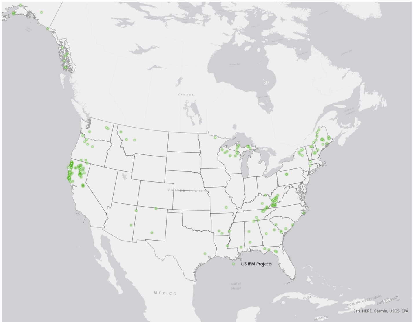
Figure 2. Location of 189 US IFM projects.

2.2.2.1 Independent verified registered project (IVRP) stock adjustments

Because all projects are on different reporting cycles, for this analysis all project IFM-1 stocks should be grown (or degrown) to match the date of the large-scale estimate to simulate a single point in time ground truth estimate. The annual growth rates were applied compounded annually for the number of fractional years between the IVRP-reported stocks and the large-scale stock reporting date. The growth rate used was estimated based on simulations using the Forest Vegetation Simulator (FVS) growth and yield model growing all plots with trees in each FVS variant forward for 10 years and calculating the average carbon stock growth (Dixon, 2002, 2022; Crookston and Dixon, 2005). This approach was chosen as a broadly representative measure of growth across the large area these large-scale frameworks are used. In addition, although geographic boundary files are required, not all IVRP shapefiles matched the reported acreage as listed in offset project listing documents. In all cases, the difference between the OPDR acres and the vector file acres was within 7.75% of the acreage reported in the OPDR. We corrected these discrepancies (based on the ratio of areas for these discrepancies) before comparing the regional inventory and the IVRP-reported stocks.

Finally, several different methods are available to calculate volume, biomass, and carbon from inventory data. For example, FVS, using the Fire and Fuels Extension, can report aboveground live carbon (and many other carbon pools) at a plot level (Rebain et al., 2022). The CARB requires the use of the component ratio level calculated at a tree level to estimate carbon stocks outside of Alaska, California, Oregon, and Washington (Compliance Offset Protocol US Forest Projects, 2015). The calculation of relative bias must use the same calculation methods as those applied in the IVRPs.

2.3 Calculating the subdomain bias discount factor

For the initial project carbon stock adjustment due to potential subdomain bias, we propose a risk-based approach that combines the distribution of IVRP stock estimates and the literature review-based distribution of potential subdomain bias. The general principle of this approach is an extension of Neeff’s (2021) proposed method and allows standard bodies or other regulatory agencies to specify the risk level they are comfortable with (Neeff, 2021).

In Neeff’s (2021) approach, the uncertainty associated with an estimate of carbon reductions or removals tons (ERTs) can be used to calculate a discount factor at a given level of risk tolerance. This approach has been adopted by both Verra and the REDD+ TREES standard (Architecture for REDD+ Transactions, 2021; Verra, 2023) (Verra is “a non-profit organization that develops and manages standards for sustainable development, climate action, and responsible business practices”; Home, 2024). REDD+ TREES is “ART’s standard for the quantification, monitoring, reporting and verification of Greenhouse Gas (GHG) emission reductions and removals from REDD+ activities at a jurisdictional and national scale” (Architecture for REDD+ Transactions, 2021). The equation below is functionally equivalent to equation 8 in Neeff (2021), the equation on page 12 of the Verra Methodology, and equation 11 in the REDD+ TREES standard. The formulation used here is as follows:

$\begin{array}{ll}d{f}_{S{D}_{var}}=\frac{\%ER{T}_{LCB}}{t_{\alpha =1-\mathit{\text{conf}}\mathit{\text{level}}\%}}\ast t_{\beta =\mathit{\text{risk}}\mathit{\text{level}}\%}& (4)\end{array}$

In this equation, the $d{f}_{S{D}_{var}}$ is the discount factor applied to ERTs due to the variability of the ERT estimate at the lower confidence bound (LCB) using a given confidence level. $d{f}_{S{D}_{var}}$ in this formulation is expressed as a percentage. $t_{\alpha =1-\mathit{\text{conf}}\mathit{\text{level}}\%}$ is the t-value of the two-sided specified confidence level (This confidence level is specified by the standard. ACR, Verra, and ART use a 90% confidence level for inventory estimates, so this would be the two-sided t-value at 10%.). This percentage difference is then scaled by the $t_{\beta =\mathit{\text{risk}}\mathit{\text{level}}\%}$ (risk value) at a chosen risk level to control for the likelihood that a given level of over-crediting risk may occur due to the variability of the ground truth data. This risk is also specified by the standard. Verra uses a 33% risk (Verra, 2023). ART uses a 30% risk (Architecture for REDD+ Transactions, 2021). ACR is using a 10% risk level for the IFM SNIPF methodology (American Carbon Registry, 2021a). The t_β value is a one-sided value as offset integrity is only concerned with over-crediting. Finally, the $\%ER{T}_{LCB}$ term represents the uncertainty of the estimate at the lower confidence bound (LCB), given the specified confidence level as a percentage of the mean reported stocks.

As with all problems of estimation and sampling, it is generally impossible to remove all risks while maintaining reasonable levels of effort, cost, and efficiency. Using a risk-based approach allows practitioners the ability to more explicitly set the appropriate level of risk and the confidence levels they are comfortable with (e.g., the inventory confidence deduction is based on an acceptable level of inventory variability and hence risk).

Equation 4 above serves as the foundation for the method described here. The Neeff approach discounts the claimed ERT based on the variability of the ERT estimate. In the case of subdomain bias, we extend this approach by treating the distribution of relative bias of the subdomain estimate as another component of the ERT estimate variability. We then can add the observed mean shift of the ground truth distribution (i.e., the bias) onto this discount factor to capture both the variability ($d{f}_{SA{E}_{var}}$) of the relative bias estimate (this variability reflects the accuracy of the large-scale inferential paradigm) and the size of the bias present (the precision of the large-scale estimate). The final discount factor calculation combines these two elements as shown in Equation 5:

$\begin{array}{ll}d{f}_{S{D}_{\mathit{\text{tot}}}}=d{f}_{S{D}_{var}}-\%ER{T}_{MS\text{.}}& (5)\end{array}$

Where the variability discount factor $d{f}_{S{D}_{var}}$ is defined above, and the $\%ER{T}_{MS}$ represents the percentage relative bias mean of ERTs. The $\%ER{T}_{MS}$ is negative when it shows the potential for over-crediting.

To calculate the relative bias for each IVRP, the first step is to apply the large-scale estimate to each IVRP within the vector file boundaries for each project. Comparing the IVRP IFM-1 stocks (grown to the date of the large-scale estimate layer) produces a relative bias percentage of the standing stocks for each project. This set of relative bias percentages is then applied to the mean stocks of the large-scale estimate layer for the full extent of the large-scale estimate. This is done as part of the process of converting the relative bias of initial carbon stocking estimates into the relative bias of ERTs. By applying the percentage relative bias at ground truth IVRP property locations to the grand mean of the large-scale estimate, we can determine both the potential variability introduced when applying a large-scale estimate to a small subdomain and we can also see the bias this may produce (all within the original large-scale estimate frame).

Once the distribution of potential large-scale estimates is calculated from the observed relative biases of all IVRPs, the distribution of potential ERT estimates is calculated by adding the difference between the original average initial stocks and the biased initial stock estimate to the original estimate of ERTs. This is done as changes in initial stocks can be considered to affect initial reductions and likely will not affect removals, i.e., the growth of the forest. In cases where the relative bias of initial stocks is negative (indicating an underestimate of stocks by the large-scale model), this will lead to under-crediting ERTs. In cases where the relative bias of initial stocks is positive (indicating an overestimate of carbon stocks by the large-scale model), this will lead to over-crediting ERTs. Table 1 shows a list of definitions that will be used throughout the steps describing this method. The full list of steps described in this method can be seen in Tables 2, 3. A flowchart that summarizes this method can be seen in Figure 3.

Table 1

Table 1. Definitions of variables used in discount factor calculation method.

Table 2

Table 2. Discount factor calculation steps for variability-only portion of discount factor df_{sd_var}.

Table 3

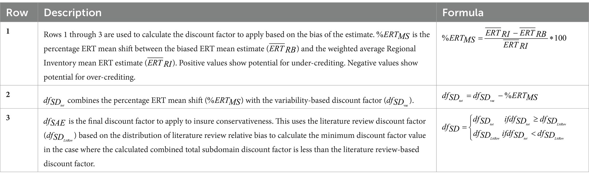
Table 3. Final calculation of discount factor based on the variability-only discount factor, the percentage mean shift, and the literature review-based discount factor calculation.

Figure 3

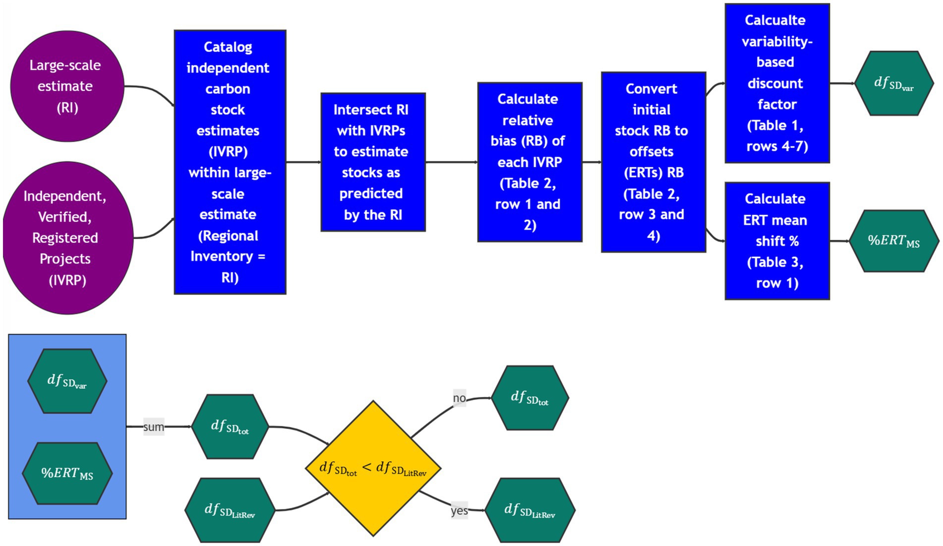
Figure 3. Subdomain bias discount factor calculation flowchart.

Example calculations for several large-scale inferential paradigms using this approach are provided in the Results and Conclusion sections to illustrate how this process is applied. That section focuses broadly on methods that generate large-scale estimates of forest attributes. By large scale, we mean state, regional, national, or global scale approaches used to quantify forest conditions. These approaches can use design- or model-based methods (or combinations of these two—e.g., composite estimates) to infer the state of forests at a given point in time. Given the scales in question, all of these methods generally require a forest inventory that provides a representative sample over the large area in question.

For model-based approaches, these data are used to train and evaluate models that predict forest attributes assuming an underlying population model. Design-based approaches use probability samples that do not assume any underlying structure to the data and instead infer population characteristics from the probability sample. National forest inventories are therefore a frequent component of large-scale inferential paradigms. For that reason, we briefly describe the structure of the NFI in the United States.

2.3.1 USFS forest inventory and analysis dataset

In the United States, the NFI is conducted by the Forest Inventory and Analysis (FIA) program (USDA Forest Service). This data source provides valuable information regarding the status of forests at regional to national scales. The sample plots are available to the public (though their exact locations are perturbed—see below). They are placed on the landscape with a sampling intensity of one plot per approximately 6,000 ac (McRoberts, 2005). The USFS FIA NFI is a random, equal probability sample. Through its design, the FIA plot network is well-suited for analyzing and quantifying forest attributes at various user-defined spatial scales (e.g., counties, states, regions, or the entire US) over time and for assessing forest changes across space. This plot network provides a basis for unbiased estimates of specific populations of interest in a consistent and timely fashion (Gray et al., 2012).

2.3.1.1 FIA plot design and measurements

The following information about the FIA program is provided as context. Most large-scale estimates (regardless of the approach used) required measured forest inventory data to train or calculate the final estimate. The FIA program adopted a standardized inventory design methodology in the year 1999 to provide uniform and consistent results across the country. They use a hexagon grid to allocate plots across all lands and ownership classes. Measurements are sorted on a panel system inside each state; thus, a subset of the state grid is measured every year. A complete cycle of panel measurement takes approximately 5 years in the eastern states and approximately 10 years in the western states. A single plot consists of a cluster of four sample points. The central plot is georeferenced, and the other three plots are located 36.6 m from the central point at 0-, 120-, and 240-degrees azimuth. A detailed description of tree individual measurements in the plots can be found in The Forest Inventory and Analysis Database description (Burrill et al., 2024).

2.3.1.2 Design-based estimates using FIA plots

Scott et al. (2005) provide documentation to obtain design-based forest attribute totals for simple random estimation, stratified estimation, and double sampling for stratification based on Phase 1 stratification. Variance estimators are also provided. The sampling error may be computed for all estimates and areas of interest although they specify that at least four plots should be included for any stratum.

2.3.1.3 Perturbed FIA coordinates

The FIA program must comply with public law prohibiting the disclosure of proprietary information. McRoberts et al. discuss why the FIA program has established additional policies of not disclosing the owner’s information and the exact location of plots (McRoberts et al., 2005). “The 2000 Interior and Related Agencies Appropriations Act (H.R.3423), which applies to information collected pursuant to Section 3(e) of the Forest and Rangelands Renewable Resources Research Act of 1978 (16U.S.C. 1,642(e)), included the FIA program in Section 1770 of the Food Security Act of 1985 (7U.S.C. 2,276)” (U.S. Code Title 16 Chapter 36 Subchapter 2 Section 1642 - Investigations, experiments, tests, and other activities - Subsection e - Forest Inventory and Analysis, 1978; U.S. Code Title 7 Chapter 55 Section 2276, 2018; de la Garza, 1985; Rep Young, 1999).

To comply with the law, FIA plot locations are perturbed (fuzzed location), and some plots are swapped with those of similar plots (similar forest type, stand size, county). All plot locations are perturbed within circular areas of radii of 1 mi. However, McRoberts et al. (2005) point out that the proportion of perturbed plots that fall more than 0.5 mi from the original location is small.

2.4 Alternative discount factor calculation form

The approach outlined above treats the variability of the sampled ground truth dataset (the IVRP population) distinctly from the mean bias observed in this population. This approach is compelling due to its simplicity and the ease of explaining how to apply the discount factor to the emission reduction tons (ERTs). Despite this simplicity, by adding the bias (% mean shift) directly to the variability-based discount factor, the above method deviates from the pure risk-based approach that Neeff outlined. An alternative approach is to use a scaled Student t-distribution method. This method allows for the selection of a risk level and for that risk to carry through the full discount factor calculation.

First, define a conservative estimate of ERT relative bias ($ER{T}_{RB,c}$). Assume the proponent uses a sample of $n$ independent ground truth carbon estimates from existing independent verified and registered carbon projects and uses these projects’ independent inventory systems to predict the carbon amount on these $n$ sites. If the proponent inventory (the regional inventory) system is unbiased, then it is expected that in half of the cases, the relative bias takes a positive value, and the other half takes a negative value. Hence, the mean of the RB project estimates ($ER{T}_{RB,\overline{x}}$) should be zero or near zero. Based on prior information collected from the literature, it is known that the distribution of $ER{T}_{RB,\overline{x}}$ is symmetric and has a shape similar to the normal distribution. A correction that makes the inventory system produce an $ER{T}_{RB,c}$, such that $ER{T}_{RB,c}=ER{T}_{RB,\overline{x}}+\mathit{\text{correction}}$, that is located to the right of the $ER{T}_{RB,\overline{x}}$, is considered conservative because the system would now be under-crediting most of the time.

As the $ER{T}_{RB,\overline{x}}$ increases (shifts to the right), the risk of over-crediting decreases. Therefore, a conservative estimate of $RB$ with a low risk of overestimation $\alpha$ is such that:

$\begin{array}{ll}P\left\{ER{T}_{RB,c}\ge 0\right\}=1-\alpha & (6)\end{array}$

To obtain a conservative $ER{T}_{RB,c}$, the $ER{T}_{RB,\overline{x}}$ needs to be shifted by a given amount ($C_{RB}$), which can be established using Equation 6 as follows:

$\begin{array}{ll}P\left\{ER{T}_{RB,\overline{x}}+C_{RB}\ge 0\right\}=1-\alpha & (7)\end{array}$

$C_{RB}=\{\begin{array}{cc}d{f}_{S{D}_{\mathit{\text{LitRev}}}}& \text{if}{\alpha }_0\le \alpha \\ t_{{\alpha }_0}^{\ast }+\mathit{\text{abs}}\left(t_{\alpha }^{\ast }\right)& \text{if}{t}_{\alpha }^{\ast }\le 0\\ t_{{\alpha }_0}^{\ast }-t_{\alpha }^{\ast }& \text{if}{t}_{{\alpha }_0}^{\ast }\ge t_{\alpha }^{\ast }\&t_{\alpha }^{\ast }\ge 0\end{array}\text{ (8)}$

where $t_{\alpha }^{\ast }=t\left(\alpha ,df,ER{T}_{RB,\overline{x}},\mathit{\text{scale}}\right)$ is the quantile of a Student t-distribution with location $ER{T}_{RB,\overline{x}}$ and scale factor $\mathit{\text{scale}}$ = standard error of $ER{T}_{RB,\overline{x}}$ (NIST/SEMATECH e-Handbook of Statistical Methods, 2023). The * represents the scaled t-distribution. $t_{{\alpha }_0}^{\ast }$ is the scaled t-value that represents the proportion of samples with negative relative bias. The three cases outlined in Equation 8 are as follows:

$\text{If }{\alpha }_0\le \alpha$

○ this case can be seen in Figure 4—Case 1 below. It represents cases where the proportion of negative RB is less than or equal to the risk level. Equivalently, $t_{{\alpha }_0}\le t_{\alpha }$. In this case, the risk of observing over-crediting is less than the defined risk threshold, and therefore, no deduction is necessary to meet the required risk tolerance. In this case, as in the primary method described above, the literature review risk level is used as the discount factor.

Figure 4

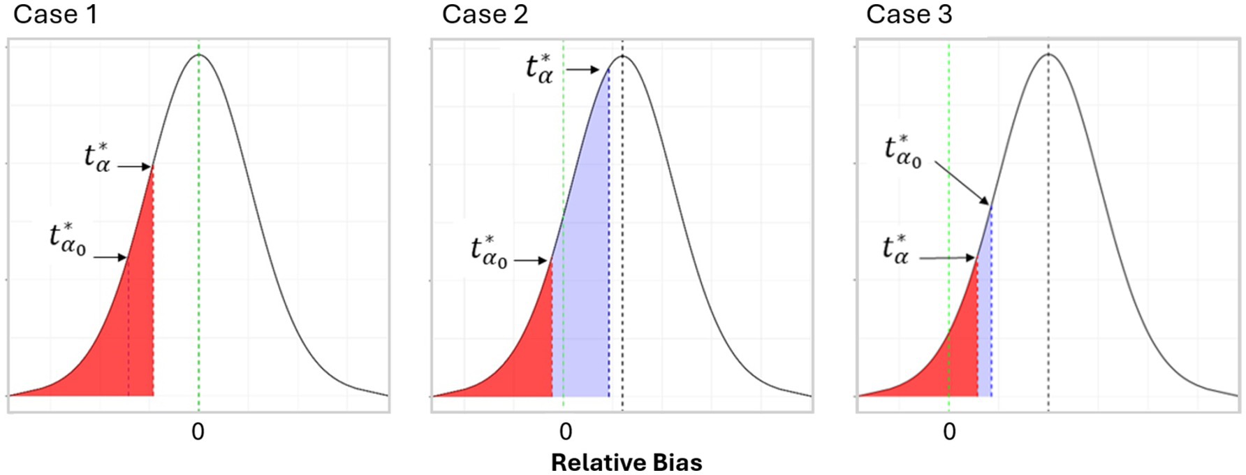
Figure 4. Example of alternative risk-based discount factor calculation method.

$\text{if }{t}_{\alpha }^{\ast }\le 0$

○ this case can be seen in Figure 4—Case 2 below. It represents cases where the t quantile that represents the risk is on the negative side of the distribution and the quantile that represents the proportion of negative RB could be in the negative or positive side of the distribution (but will always be larger than $t_{\alpha }^{\ast }$). In this case, to guarantee that the risk of over-crediting is less than or equal to α, we apply a discount factor. As a result, the discount factor is the net distance between the two quantiles. It is obtained by adding the absolute value of the scaled risk t-value to the scaled proportion of negative project t-value. Where there are higher proportions of negative relative bias values, this results in larger discount factors.

if $t_{{\alpha }_0}^{\ast }\ge t_{\alpha }^{\ast }\&t_{\alpha }^{\ast }\ge 0$

○ this can be seen in Figure 4—Case 3 below. It represents cases where the mean relative bias is positive and the t quantile for the risk level is positive, but still, the proportion of negative RB is larger than the risk level chosen. As a result, the deduction is the linear distance (or simple subtraction) between $t_{{\alpha }_0}^{\ast }$ and $t_{\alpha }^{\ast }$.

Figure 4 is a representation of various scenarios where the t quantile associated with the selected risk is compared with the t quantile linked to the sampled proportion of negative RB. The sign of these two elements needs to be considered when calculating the linear distance between them. This distance is then used as a measure of the deduction.

Note that for the two last cases in Equation 8, the formulas calculate the linear distance between the two t-values. This is the linear distance in relative bias space between the t-value for the specified risk and the t-value for the distribution portion equivalent to the sample fraction with negative relative values.

Equation 9 below shows how to calculate the quantiles $t_{\alpha }^{\ast }$ and $t_{{\alpha }_0}^{\ast }$ (Gelman et al., 2021).

$\begin{array}{ll}{t}_{\alpha }^{\ast }=ER{T}_{RB,\overline{x}}+\mathit{\text{scale}}\ast t\left(\alpha ,df\right)& (9)\end{array}$

where $t\left(\alpha ,df\right)$ is the quantile function for the t-distribution with $df$ ($df>1$) degrees of freedom.

Note that Equations 6, 7 are adaptations of equations 6–8 from the Neeff paper (Neeff, 2021).

In this formulation, $C_{RB}$ represents the adjusted amount that $ER{T}_{RB,\overline{x}}$ must be moved to have an acceptable risk of overestimation of $\alpha$. This adjustment is calculated based on the distance between the two Student t quantiles.

The deduction factor needed for emission reductions is assumed to be proportional to $C_{RB}$. That is, as Equation 10 explains, the deduction factor needs to adjust the emission reduction (ERTs) to account for possible over-crediting when estimates are done on subdomains is:

$\begin{array}{ll}ERT{s}_{adj}^{\ast }=\mathit{\text{ERTs}}\ast \left(1-C_{RB}\right)& (10)\end{array}$

Therefore, the alternative deduction factor is $\left(1-C_{RB}\right)\text{.}$

3 Results

3.1 Literature review results

Figure 5 shows the results of those studies that published both the prediction for a small area and the observed direct measurement of the same small area. While some studies produce results for large regions (e.g., the entire country and small areas within this country), other studies are more targeted to states and small areas within these states or even counties or ownerships and small areas within these areas. The list of all papers reviewed (over 60) that were considered in this analysis can be found in the References section at the end of this document.

Figure 5

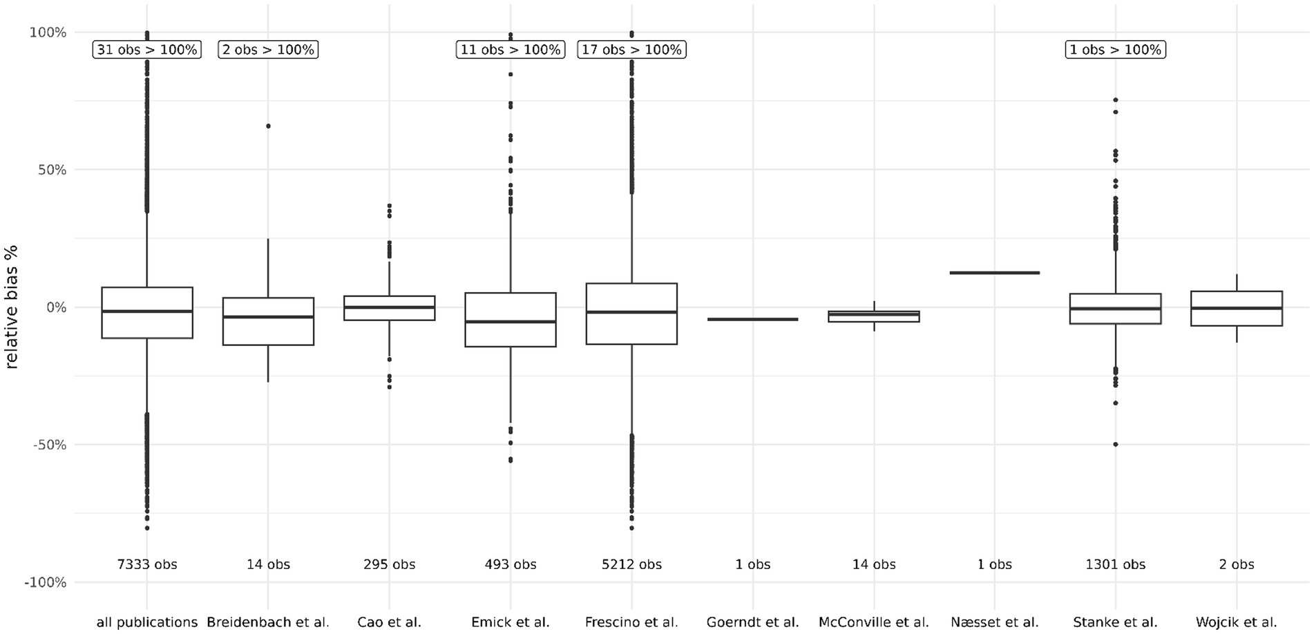
Figure 5. Distribution of relative bias from published literature. The leftmost boxplot shows all data together.

Table 4 shows the range of potential RB in 10 studies. These 10 studies resulted in 7333 datapoints that can be used to understand the expected distribution of RB. All but 4 of these 7,333 datapoints were actual estimates of small areas that also had a direct sample. The 4 remaining were only reported as the mean or were taken from a spread of points in a graph and used the min and max. Of these 7,333 datapoints, 6,823 were from composite models (SAE models), 493 were from model-based estimates, and 17 were from model-assisted estimates. Tables 5, 6 summarize these results:

Table 4

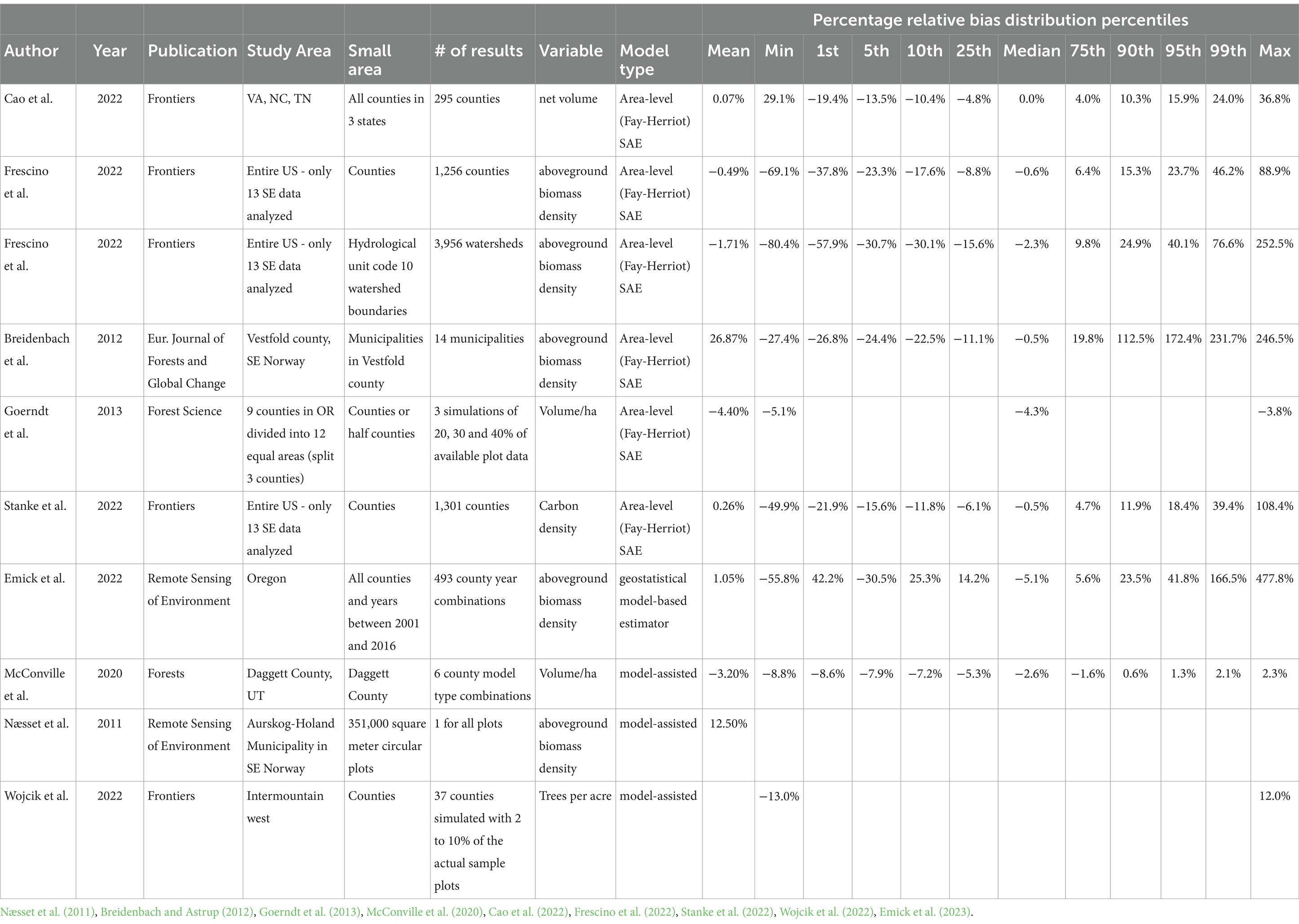
Table 4. Relative bias estimated from published literature.

Table 5

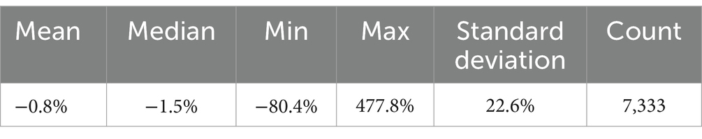
Table 5. Distribution of relative bias from data reported in published literature.

Table 6

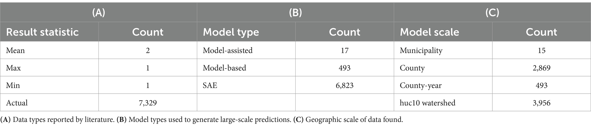
Table 6. Breakdown of published relative bias data by type.

The results of this literature review show one realization of potential bias and the uncertainty of this bias when applying a large-scale inferential paradigm to a subdomain. These results can be used to understand the distributional properties of RB and how large in magnitude a correction factor should be to obtain conservative forest attribute estimates.

3.2 Example 1: design-based stratified regional estimate

Consider the scenario where a large geographic area is broken into logical populations that reflect attributes of interest, e.g., regulatory constraints or ecological similarity. Then, a suite of remote sensing data products is combined to generate a stratification of forest land over each of these independent population areas. This stratification is then paired with an existing NFI such as the USFS FIA dataset to generate stratum level estimates that the NFI was designed to measure. Given a random or systematic grid of plot locations, this pairing of plot data with the stratification is considered a post-stratification for each independent population.

Furthermore, imagine that this large-scale inventory is the basis for the quantification of forest carbon offsets (ERTs) at the landowner scale. Given this structure, Tables 2, 3 show the formulae that describe the calculation of a discount factor to be applied to ERTs issued using the approach outlined above. Table 7 shows a worked example of this approach.

Table 7

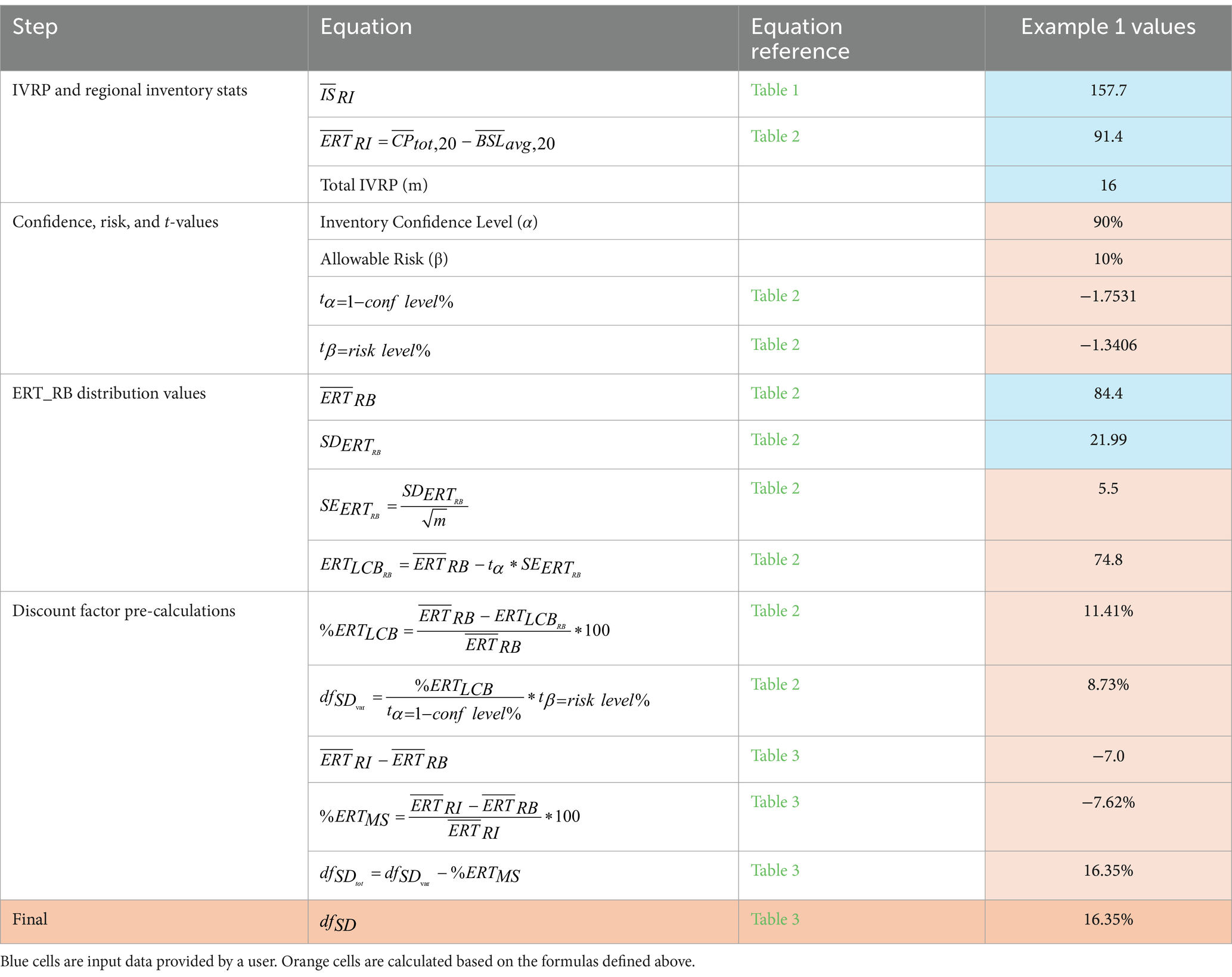
Table 7. Worked Example 1—Discount factor for large over-crediting risk from design-based regional inventory.

A graphical representation of the calculated discount factor can be seen in Figure 6A below.

Figure 6

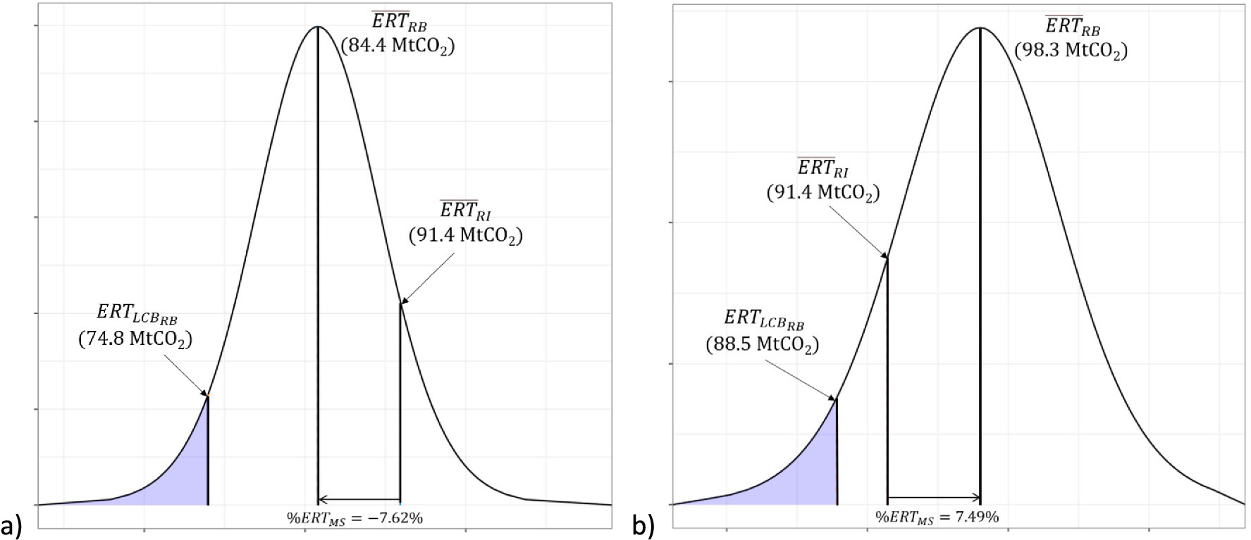
Figure 6. Graphical representation of examples 1 and 2. (A) Shows the design-based large over-crediting risk. In this figure, the initial stocks as estimated by the IVRP data were 7.62% less than the stocks estimated by the regional inventory (RI). This difference, combined with the variability-based discount, results in a 16.35% final ERT deduction factor. (B) Shows the minimal over-crediting risk associated with a model-based estimate of regional inventory stocks. The initial stock underestimate by the regional inventory results in a conservative estimate of ERTs and therefore a small discount factor.

3.3 Example 2: model-based regional estimate

The second example considers a case where a regional- or national-scale model-based estimate is used to predict initial carbon stocks, and this prediction is then used for carbon offset credit generation. In this case, assume the model is applied at a 30 m pixel level across the full project region. By adding up all pixel values and dividing them by the number of pixels, the regional inventory mean is found. A similar process as above is then applied to these results to adjust any small area over-crediting bias.

Table 8 below shows a worked example of a model-based approach. There are two notes to consider for this example:

1. The process is the same regardless of the estimation approach, i.e., model-based or design-based.

2. The example below shows a scenario with minimal over-crediting risk. Therefore, this example uses the literature review-based discount factor adjustment.

Table 8

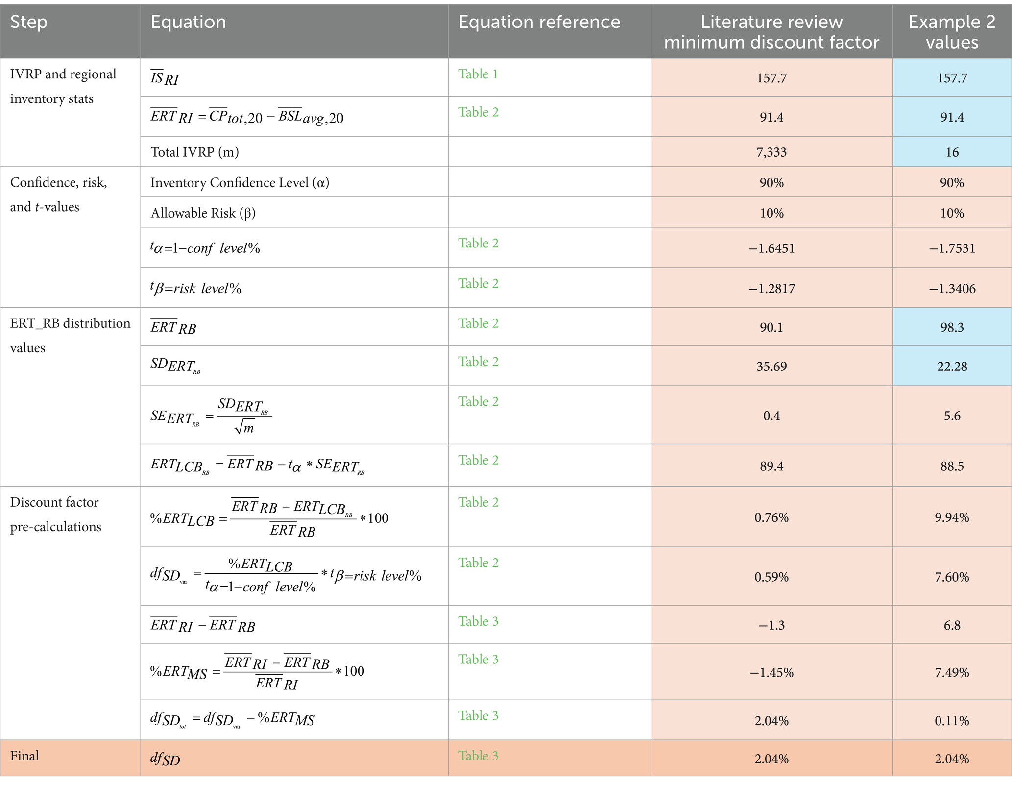
Table 8. Worked example 2—discount factor calculation for minimal over-crediting risk using the literature review results for the discount factor.

Figure 6B shows a graphical example of the discount factor adjustment calculated for example 2. In example 1, the mean ERTs when accounting for relative bias are less than the ERTs estimated in the large-scale design-based framework. In example 2, this is reversed (note the negative $\%ER{T}_{MS}$ in example 1 and the positive $\%ER{T}_{MS}$ in example 2). As a result of this difference, when subtracting the negative % from the variability discount factor, the result is less than the minimum discount factor as defined by the literature review results. As a result, in example 2, the final discount factor to be applied to the ERTs generated will be the literature review calculated discount factor. As described above, this serves as the minimum possible discount factor to protect against shortcomings based on the small sample size of the IVRP analysis.

4 Discussion

The examples above show the steps required to calculate and apply the discount factor to prevent over-crediting when using a large-scale inferential framework for smaller internal subdomains. Using this method, we treat any subdomain bias measured for the initial stock estimate as equivalent to a bias in the claimed ERTs. Said another way, if a bias in initial stocks exists, it impacts avoided emissions (reductions) instead of removals (growth).

Although only verified and issued project stocks were considered, there are still several possible problems with both the growth and area scaling adjustments. For the growth adjustment, even if we were growing for just 1 year, this assumes that no disturbances have occurred which might bias the results. Similarly, scaling the area of projects assumes that all area differences come from average stocked areas. In fact, proponents may have updated their shapefiles to remove all low stocked areas or any non-random update and this would result in a biased and inaccurate estimate. Despite these concerns, this comparison provides a robust set of 3^rd party verified carbon stocks and is the best available dataset to answer the question at hand. In addition, because of the inclusion of the variability discount, smaller datasets will result in larger deductions. This feature further protects against over-crediting.

Another potential problem with this method is that although it provides a reasonable estimate of potential bias, it cannot estimate the actual bias of the subdomains enrolled. If there is a bias in the independent projects, this may lead to biases in the estimate of potential subdomain bias and in the calculated discount factors. That said, the fact that the independent projects are also carbon projects supports the idea that these areas may represent other potential carbon project areas accurately. Further study and ground truth data to verify the findings and methods introduced here are needed to provide additional confidence in this approach.

A comparison of the original method described above and the alternative discount calculation method can be seen in Figure 7. The SE panels in Figure 7 represent the variability of the IVPR RB estimates. Because the first method relies on the variance and bias of the IVRP while the alternate method relies on the variance and proportion of the IVRP sites that have a negative relative bias, it is not possible to exactly compare these. Therefore, to make the comparison below, the average proportion of negative relative bias values was found based on 100 simulations of the distribution of possible site relative bias values based on the assumed mean bias and variance percentages. The simulations were drawn from a normal distribution. There are a few points to take from these results. First, the first proposed method (and the method adopted and published by the American Carbon Registry for use in the SNIPF methodology) results in larger discount factors as the negative bias (risk of over-crediting) increases, while the alternate method shows larger deductions even when the average bias is positive. Given the increased conservatism of the alternative method for small or no over-crediting bias situations, it is possible to remove the literature review portion of this calculation entirely. Removing this calculation will make the application of this method simpler and more internally consistent. Equation 11 shows this revised formulation.

Figure 7

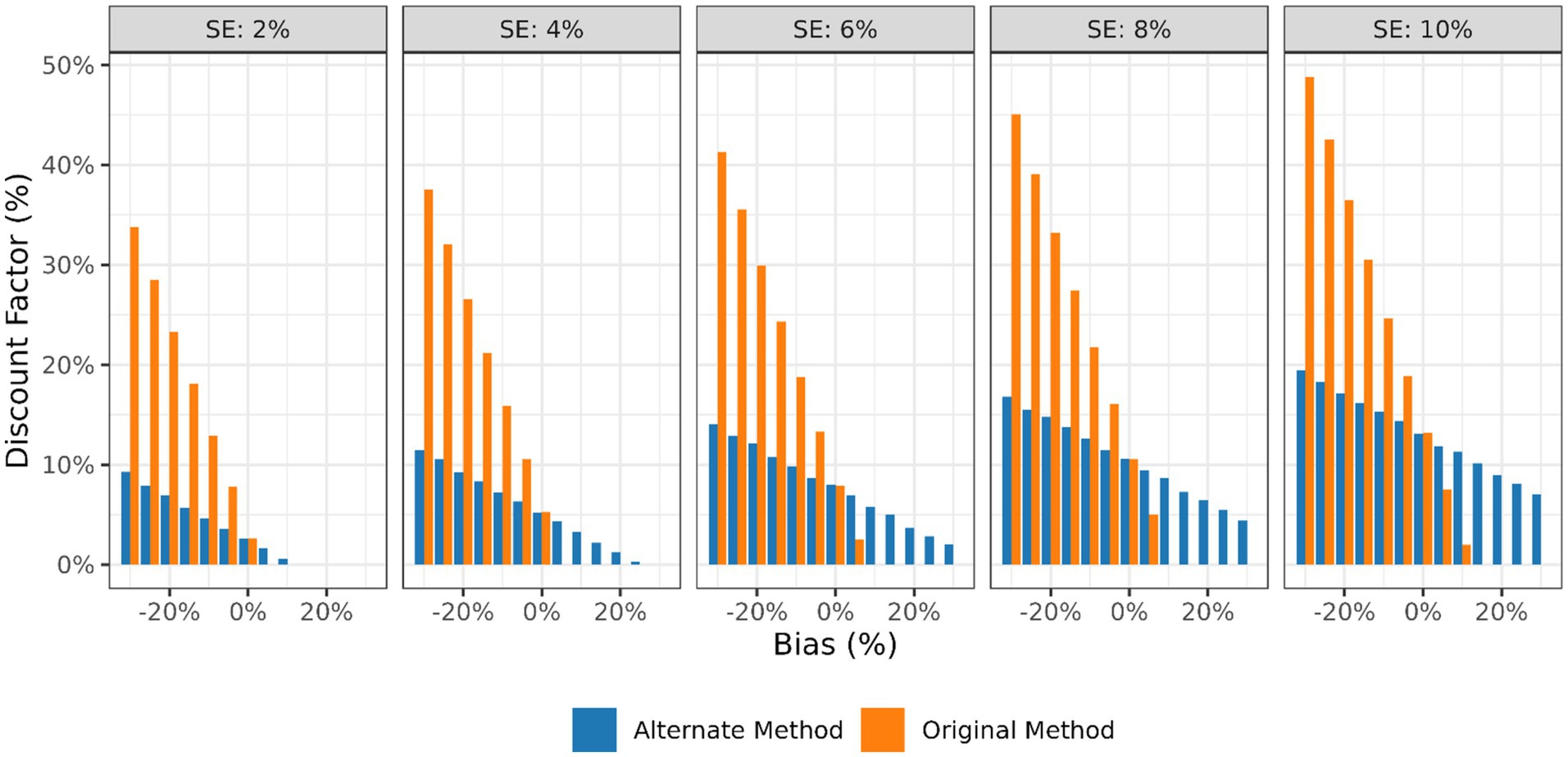
Figure 7. Comparison of original and alternate discount factor calculation methods.

Equation 11: Alternative discount factor calculation removing literature review result dependency

$C_{RB}=\{\begin{array}{cc}0& \text{if}{\alpha }_0\le \alpha \\ t_{{\alpha }_0}^{\ast }+\mathit{\text{abs}}\left(t_{\alpha }^{\ast }\right)& \text{if}{t}_{\alpha }^{\ast }\le 0\\ t_{{\alpha }_0}^{\ast }-t_{\alpha }^{\ast }& \text{if}{t}_{{\alpha }_0}^{\ast }\ge t_{\alpha }^{\ast }\&t_{\alpha }^{\ast }\ge 0\end{array}\text{ (11)}$

Further comparison of these methods reveals that the first method presents a strong relationship between the mean bias and the final deduction claimed while the alternative method relies on the proportion of negative relative bias values—which is a proxy for the mean relative bias but slightly different. The strength of the original method is its relative simplicity in incorporating the mean relative bias into the final discount factor value. The strength of the alternative method is that it more closely aligns with the risk-based framework proposed originally by Neeff. The choice of approach will be dictated by the goals of the standards body.

5 Conclusion

This paper outlines a discount factor that can be applied to estimates of carbon offsets when a large-scale estimate framework is used to estimate offsets within a subdomain. Although this publication uses an example dataset from the Southeastern United States and is specific to the ACR SNIPF IFM protocol (this method was adopted by this protocol), the intent of this study is to introduce a method that can be applied in any forest type or geography using any forest carbon offset protocol where there exist independent estimates of forest carbon stocks that overlap with the large-scale estimates. The approach breaks down the discount factor into three main components: (1) a variability-based discount factor, (2) a mean shift discount component, and (3) the discount factor associated with a review of relevant literature. By combining these components, this approach insures a conservative estimate of credit generation by projects. Using this approach, standard bodies can confidently develop offset protocols to ensure the conservativeness of offsets generated while also allowing for cutting-edge remote sensing technologies to be deployed to allow for the rapid scaling of program participation.

While this method is specific to forests and forest carbon offsets, the general framework could easily be adapted to work in other fields or for other purposes. For example, if one wanted to estimate soil contamination in small areas based on a larger-scale estimate where robust subdomain observations were available, this method could be applied. Furthermore, if one was more concerned with underestimation rather than overestimation, the signs in the formulas could be reversed to address this risk instead.

Because this method relies on independent projects to understand the potential subdomain estimation variance and bias, it is the opinion of the authors that registries and standards bodies should try to follow the lead of the CARB in requiring project area shapefiles and standing carbon stocks be made publicly available for all forest carbon offset projects at each verification. Furthermore, verifiers and registries should take care to ensure that provided project area vector files remain consistent with the actual project area as defined in the project reporting documents. Finally, the certainty of the inventory estimates should be reported to allow for a more detailed analysis of the potential bias of large-scale forest estimation frameworks.

Some may argue that the standard body should not allow any known bias or increased variance in estimates of carbon stocks and ERTs. They may further argue that all forest-based climate solutions must therefore rely on direct, ground-based samples of stocks. We believe that there is an inherent trade-off between the cost of offset project development and the participation in these projects. Because ground-based approaches become cost prohibitive when projects span large geographic extents and include many disjoint enrolled polygons, this method to account for and mitigate potential increased variability and bias is critical to improving participation in these programs and in increasing the climate and ecosystem co-benefits these programs create.

Addressing climate change and protecting forests is an immense challenge. The IPCC estimates that there is an “emissions gap” of 4 to 7 GtCO₂ needed to reduce emissions and help to stabilize warming below 1.5°C (Core Writing Team, 2023). Given the size of this emissions gap and the importance of protecting forests, it is critical that we develop tools that incentive forestland protection and can do so with high integrity at large scales. By providing a method to adjust for both the variability and bias that subdomain estimates might introduce, this method opens the door to the use of more efficient large-scale models and estimation frameworks to reduce costs for participants in forest carbon offset programs while maintaining high-integrity offsets.

Data availability statement

Publicly available datasets were analyzed in this study. This data can be found here: https://thereserve2.apx.com/myModule/rpt/myrpt.asp?r=211 and https://acr2.apx.com/myModule/rpt/myrpt.asp?r=111.

Author contributions

JG: Conceptualization, Data curation, Formal analysis, Investigation, Methodology, Project administration, Resources, Software, Supervision, Validation, Visualization, Writing – original draft, Writing – review & editing. MZ-C: Conceptualization, Formal analysis, Investigation, Methodology, Software, Validation, Visualization, Writing – review & editing. EW: Conceptualization, Data curation, Investigation, Project administration, Validation, Writing – review & editing. AB: Data curation, Investigation, Visualization, Writing – review & editing. DO’L: Conceptualization, Data curation, Software, Writing – review & editing. RK: Conceptualization, Methodology, Software, Writing – review & editing. WM: Conceptualization, Formal analysis, Investigation, Software, Writing – review & editing.

Funding

The author(s) declare that no financial support was received for the research, authorship, and/or publication of this article.

Acknowledgments

The authors would like to acknowledge the detailed and comprehensive feedback provided by the reviewers of this manuscript. Furthermore, we’d like to thank the American Carbon Registry, and specifically Kurt Krapfl, Andrew Taylor, and Gabriel Burns, for their support and consultation as we developed this approach. Till Neeff was also gracious with his time and feedback and provided the foundation that we used to build this approach. John Kershaw and Kim Iles also helped in the framing of this problem and in brainstorming potential approaches to consider. Lastly, we’d like to thank all our colleagues at Finite Carbon for their help and support in vetting this approach and providing data and suggestions during the development process.

Conflict of interest

JG, MZ-C, EW, AB, DO’L, RK, and WM were employed by company Finite Carbon.

Publisher’s note

All claims expressed in this article are solely those of the authors and do not necessarily represent those of their affiliated organizations, or those of the publisher, the editors and the reviewers. Any product that may be evaluated in this article, or claim that may be made by its manufacturer, is not guaranteed or endorsed by the publisher.

References

American Carbon Registry (2021a). Errata and clarifications of the improved Forest management on small non-industrial private forestlands. North Little Rock, AR: American Carbon Registry.

Google Scholar

American Carbon Registry (2021b). Methodology for the quantification, monitoring, reporting and verification of greenhouse gas emissions reductions and removals from small non-industrial private forestlands. North Little Rock, AR: American Carbon Registry.

Google Scholar

American Carbon Registry (2023a) Improved Forest management. American Carbon Registry. Available at: https://acrcarbon.org/wp-content/uploads/2023/03/Improved-Forest-Management-Primer.pdf (Accessed April 9, 2024).

Google Scholar

American Carbon Registry (2023b). The ACR standard: Requirements and specifications for the quantification, monitoring, reporting, verification, and registration of project-based Ghg emissions reductions and removals. North Little Rock, AR: Winrock International.

Google Scholar

American Carbon Registry Registry (2024). Available at: https://acr2.apx.com/myModule/rpt/myrpt.asp?r=111 (Accessed April 25, 2024).

Google Scholar

Architecture for REDD+ Transactions (2021) The REDD+ environmental excellence standard (TREES). Architecture for REDD+ Transactions (ART). Available at: https://www.artredd.org/wp-content/uploads/2021/12/TREES-2.0-August-2021-Clean.pdf (Accessed April 25, 2024).

Google Scholar

Babcock, C., Finley, A., Andersen, H. E., Pattison, R., Cook, B., Morton, D., et al. (2018). Geostatistical estimation of forest biomass in interior Alaska combining Landsat-derived tree cover, sampled airborne lidar and field observations. Remote Sens. Environ. 212, 212–230. doi: 10.1016/j.rse.2018.04.044

Crossref Full Text | Google Scholar

Badgely, G., Freeman, J., Hamman, J. J., Haya, B., and Cullenward, D. (2021). California improved forest management offset project database. Zenodo. doi: 10.5281/zenodo.4630684

Crossref Full Text | Google Scholar

Bell, D. M., Wilson, B., Werstak, C. Jr., Oswalt, C., and Perry, C. (2022). Examining k-nearest neighbor small area estimation across scales using National Forest Inventory Data. Front. Forests Global Change 5. doi: 10.3389/ffgc.2022.763422

Crossref Full Text | Google Scholar

Breidenbach, J., and Astrup, R. (2012). Small area estimation of forest attributes in the Norwegian National Forest Inventory. Eur. J. For. Res. 131, 1255–1267. doi: 10.1007/s10342-012-0596-7

Crossref Full Text | Google Scholar

Breidenbach, J., Magnussen, S., Rahlf, J., and Astrup, R. (2018). Unit-level and area-level small area estimation under heteroscedasticity using digital aerial photogrammetry data. Remote Sens. Environ. 212, 199–211. doi: 10.1016/j.rse.2018.04.028

Crossref Full Text | Google Scholar

Bullock, E. L., Woodcock, C., Souza, C. Jr., and Olofsson, P. (2020). Satellite-based estimates reveal widespread forest degradation in the Amazon. Glob. Chang. Biol. 26, 2956–2969. doi: 10.1111/gcb.15029

PubMed Abstract | Crossref Full Text | Google Scholar

Burrill, E. A., Christensen, G. A., Conkling, B. L., DiTommaso, A. M., Lepine, L., Perry, C. J., et al. (2024) The Forest inventory and analysis database - FIADB user guides - volume: Database description (version 9.2), nationwide forest inventory (NFI). User guide 04.2024. USDA Forest Service, p. 1042. Available at: https://www.fs.usda.gov/research/understory/forest-inventory-and-analysis-database-user-guide-nfi (Accessed April 25, 2024).

Google Scholar

Cao, Q., Dettmann, G., Radtke, P., Coulston, J., Derwin, J., Thomas, V., et al. (2022). Increased precision in county-level volume estimates in the United States National Forest Inventory with Area-Level Small Area Estimation. Front. Forests Global Change 5, 1–13. doi: 10.3389/ffgc.2022.769917

Crossref Full Text | Google Scholar

Climate Action Reserve (2019). Key accounting principles for improved Forest management projects within the Forest protocol. Climate Action Reserve. 13, 1–13.

Google Scholar

Climate Action Reserve (2023). U.S. Forest protocol. Los Angeles, CA: Climate Action Reserve.

Google Scholar

Climate Action Reserve Registry (2024). Available at: https://thereserve2.apx.com/mymodule/mypage.asp (Accessed April 25 2024).

Google Scholar

Cohen, W. B., Healey, S., Yang, Z., Stehman, S., Brewer, C., Brooks, E., et al. (2017). How similar are Forest disturbance maps derived from different Landsat time series algorithms? Forests 8:98. doi: 10.3390/f8040098

Crossref Full Text | Google Scholar

Compliance Offset Protocol US Forest Projects (2015). California Environmental Protection Agency air resources board. Available at: https://ww2.arb.ca.gov/our-work/programs/compliance-offset-program/compliance-offset-protocols/us-forest-projects/2015 (Accessed April 8, 2024).

Google Scholar

Core Writing Team (2023). Climate change 2023: Synthesis report. Contribution of working groups I, II and III to the sixth assessment report of the intergovernmental panel on climate change. Geneva, Switzerland: IPCC.

Google Scholar

Corona, P., Fattorini, L., Franceschi, S., Scrinzi, G., and Torresan, C. (2014). Estimation of standing wood volume in forest compartments by exploiting airborne laser scanning information: model-based, design-based, and hybrid perspectives. Can. J. For. Res. 44, 1303–1311. doi: 10.1139/cjfr-2014-0203

Crossref Full Text | Google Scholar

Coulston, J. W., Green, P., Radtke, P., Prisley, S., Brooks, E., Thomas, V., et al. (2021). Enhancing the precision of broad-scale forestland removals estimates with small area estimation techniques. Forestry 94, 427–441. doi: 10.1093/forestry/cpaa045

Crossref Full Text | Google Scholar

Crookston, N. L., and Dixon, G. E. (2005). The forest vegetation simulator: a review of its structure, content, and applications. Comput. Electron. Agric. 49, 60–80. doi: 10.1016/j.compag.2005.02.003

Crossref Full Text | Google Scholar

Curtis, P. G., Slay, C., Harris, N., Tyukavina, A., and Hansen, M. (2018). Classifying drivers of global forest loss. Science 361, 1108–1111. doi: 10.1126/science.aau3445

PubMed Abstract | Crossref Full Text | Google Scholar

de la Garza, E. (1985) Food security act of 1985, H.R. Available at: https://www.congress.gov/bill/99th-congress/house-bill/2100 (Accessed April 25, 2024).

Google Scholar

Dettmann, G. T., Radtke, P. J., Coulston, J. W., Green, P. C., Wilson, B. T., and Moisen, G. G. (2022). Review and synthesis of estimation strategies to meet small area needs in Forest inventory. Front. Forests Global Change 5:813569. doi: 10.3389/ffgc.2022.813569

Crossref Full Text | Google Scholar

Dixon, G. E. (2002) A User’s guide to the Forest vegetation simulator, 226.

Google Scholar

Dixon, G. (2022) Essential FVS: A User’s guide to the Forest vegetation simulator. United States Department of Agriculture, Forest Service, Forest Management Service Center. Available at: https://www.fs.usda.gov/fmsc/ftp/fvs/docs/gtr/EssentialFVS.pdf

Google Scholar

Emick, E., Babcock, C., White, G., Hudak, A., Domke, G., and Finley, A. (2023). An approach to estimating forest biomass while quantifying estimate uncertainty and correcting bias in machine learning maps. Remote Sens. Environ. 295:113678. doi: 10.1016/j.rse.2023.113678

Crossref Full Text | Google Scholar

Fitts, L. A., Russell, M., Domke, G., and Knight, J. (2021). Modeling land use change and forest carbon stock changes in temperate forests in the United States. Carbon Balance Manag. 16:20. doi: 10.1186/s13021-021-00183-6

PubMed Abstract | Crossref Full Text | Google Scholar

Frescino, T. S., McConville, K. S., White, G. W., Toney, J. C., and Moisen, G. G. (2022). Small area estimates for National Applications: a database to dashboard strategy using FIESTA. Front. Forests Global Change 5:779446. doi: 10.3389/ffgc.2022.779446

Crossref Full Text | Google Scholar

Gelman, A., Carlin, J. B., Stern, H. S., Dunson, D. B., Vehtari, A., and Rubin, D. B. (2021). Bayesian data analysis. 3rd Edn. Chapman and Hall/CRC. Available at: https://stat.columbia.edu/~gelman/book/BDA3.pdf

Google Scholar

Goerndt, M. E., Monleon, V., and Temesgen, H. (2011). A comparison of small-area estimation techniques to estimate selected stand attributes using LiDAR-derived auxiliary variables. Can. J. For. Res. 41, 1189–1201. doi: 10.1139/x11-033

Crossref Full Text | Google Scholar

Goerndt, M. E., Monleon, V. J., and Temesgen, H. (2013). Small-area estimation of county-level Forest attributes using ground data and remote sensed auxiliary information. For. Sci. 59, 536–548. doi: 10.5849/forsci.12-073

Crossref Full Text | Google Scholar

Gray, A., Brandeis, T., Shaw, J., McWilliams, W., and Miles, P. (2012). Forest inventory and analysis database of the United States of America (FIA). Biodiversity Ecol. 4, 225–231. doi: 10.7809/b-e.00079

Crossref Full Text | Google Scholar

Green, P. C., Burkhart, H., Coulston, J., and Radtke, P. (2020). A novel application of small area estimation in loblolly pine forest inventory. Forestry 93, 444–457. doi: 10.1093/forestry/cpz073

Crossref Full Text | Google Scholar

Gregoire, T. G. (1998). Design-based and model-based inference in survey sampling: appreciating the difference. Can. J. For. Res. 28, 1429–1447. doi: 10.1139/x98-166

Crossref Full Text | Google Scholar

Gregoire, T. G., Ståhl, G., Næsset, E., Gobakken, T., Nelson, R., and Holm, S. (2011). Model-assisted estimation of biomass in a LiDAR sample survey in Hedmark County, Norway. Can. J. For. Res. 41, 83–95. doi: 10.1139/X10-195

Crossref Full Text | Google Scholar

Guldin, R. W. (2021). A systematic review of small domain estimation research in forestry during the twenty-first century from outside the United States. Front. Forests Global Change 4:695929:10.3389/ffgc.2021.695929.

Google Scholar

Hansen, M. C., Potapov, P., Moore, R., Hancher, M., Turubanova, S., Tyukavina, A., et al. (2013). High-resolution global maps of 21st-century Forest cover change. Science 342, 850–853. doi: 10.1126/science.1244693

PubMed Abstract | Crossref Full Text | Google Scholar

Holdaway, R. J., McNeill, S., Mason, N., and Carswell, F. (2014). Propagating uncertainty in plot-based estimates of Forest carbon stock and carbon stock change. Ecosystems 17, 627–640. doi: 10.1007/s10021-014-9749-5

Crossref Full Text | Google Scholar

Home. (2024). Verra. Available at: https://verra.org/ (Accessed December 16, 2024).

Google Scholar

Justice, C., Townshend, J., Holben, B., and TUCKER, C. (1985). Analysis of the phenology of global vegetation using meteorological satellite data. Int. J. Remote Sens. 6, 1271–1318. doi: 10.1080/01431168508948281

Crossref Full Text | Google Scholar

Karnik, A., Kilbride, J. B., Goodbody, T. R. H., Ross, R., and Ayrey, E. (2024) An open-access database of nature-based carbon offset project boundaries. Research Square. Available at: https://doi.org/10.21203/rs.3.rs-4535931/v1

Google Scholar

Katila, M. (2006). Empirical errors of small area estimates from the multisource National Forest Inventory in eastern Finland. Silva Fennica 40, 729–742. doi: 10.14214/sf.324

Crossref Full Text | Google Scholar

Lin, J., Gamarra, J., Drake, J., Cuchietti, A., and Yanai, R. (2023). Scaling up uncertainties in allometric models: how to see the forest, not the trees. For. Ecol. Manag. 537:120943. doi: 10.1016/j.foreco.2023.120943

Crossref Full Text | Google Scholar

Magnussen, S., Mauro, F., Breidenbach, J., Lanz, A., and Kändler, G. (2017). Area-level analysis of forest inventory variables. Eur. J. For. Res. 136, 839–855. doi: 10.1007/s10342-017-1074-z

PubMed Abstract | Crossref Full Text | Google Scholar

Mauro, F., Monleon, V., Temesgen, H., and Ford, K. (2017). Analysis of area level and unit level models for small area estimation in forest inventories assisted with LiDAR auxiliary information. PLoS One 12:e0189401. doi: 10.1371/journal.pone.0189401

PubMed Abstract | Crossref Full Text | Google Scholar

McConville, K. S., Breidt, F., Lee, T., and Moisen, G. (2017). Model-assisted survey regression estimation with the lasso. J. Survey Statistics Methodol. 5, 131–158. doi: 10.1093/jssam/smw041

Crossref Full Text | Google Scholar

McConville, K. S., Moisen, G. G., and Frescino, T. S. (2020). A tutorial on model-assisted estimation with application to Forest inventory. Forests 11:244. doi: 10.3390/f11020244

Crossref Full Text | Google Scholar

McNulty, S., Wiener, S., Treasure, E., Myers, J. M., Farahani, H., Marshall, D., et al. (2015). USDA southeast regional climate hub assessment of climate change vulnerability and adaptation and mitigation strategies | CAKE: Climate adaptation knowledge exchange. Southeast Hub, Raleigh, NC: United States Department of Agriculture.

Google Scholar

McRoberts, R. E. (2005). “The enhanced Forest inventory and analysis program” in The enhanced forest inventory and analysis program - national sampling design and estimation procedures. eds. W. A. Bechtold and P. L. Patterson (Asheville, NC: U.S. Department of Agriculture, Forest Service, Southern Research Station).

Google Scholar

McRoberts, R. E., Næsset, E., Saatchi, S., Liknes, G., Walters, B., and Chen, Q. (2019). Local validation of global biomass maps. Int. J. Appl. Earth Obs. Geoinf. 83:101931. doi: 10.1016/j.jag.2019.101931

Crossref Full Text | Google Scholar

McRoberts, R. E., Holden, G. R., Nelson, M. D., Liknes, G. C., and Gormanson, D. D. (2005). Using satellite imagery as ancillary data for increasing the precision of estimates for the Forest inventory and analysis program of the USDA Forest Service. Canadian Journal of Forest Research, 36, 13.

Google Scholar

Næsset, E., Gobakken, T., Solberg, S., Gregoire, T., Nelson, R., Ståhl, G., et al. (2011). Model-assisted regional forest biomass estimation using LiDAR and InSAR as auxiliary data: a case study from a boreal forest area. Remote Sens. Environ. 115, 3599–3614. doi: 10.1016/j.rse.2011.08.021

Crossref Full Text | Google Scholar

Nedd, R., and Anandhi, A. (2022). Land use changes in the southeastern United States: quantitative changes, drivers, and expected environmental impacts. Land 11:2246. doi: 10.3390/land11122246

Crossref Full Text | Google Scholar

Neeff, T. (2021). What is the risk of overestimating emission reductions from forests – and what can be done about it? Clim. Chang. 166:26. doi: 10.1007/s10584-021-03079-z

Crossref Full Text | Google Scholar

NIST/SEMATECH e-Handbook of Statistical Methods (2023). National Institute of Standards and Technology, p. 2333

Google Scholar

Núñez, F., and Pavley, F. (2006) Assembly bill 32, California Global Warming Solutions Act of 2006. Available at: https://leginfo.legislature.ca.gov/faces/billNavClient.xhtml?bill_id=200520060AB32 (Accessed April 24, 2024).

Google Scholar

Order of the Minister of the Environment, the Fight Against Climate Change, Wildlife and Parks dated 17 November 2022 (2021) chapter Q-2, ss. 46.1, 46.5 and 46.8.2. Available at: https://www.publicationsduquebec.gouv.qc.ca/fileadmin/gazette/pdf_encrypte/lois_reglements/2022A/106043.pdf (Accessed April 8, 2024).

Google Scholar

Rao, J. N. K., and Molina, I. (2015). Small area estimation. Second Edn. Hoboken, New Jersey: John Wiley & Sons Inc.

Google Scholar

RCW 70A.45.020: Greenhouse gas emissions reductions—Reporting requirements. (2023) RCW 70A.45.0202. Available at: (https://apps.leg.wa.gov/rcw/default.aspx?cite=70A.45.020)

Google Scholar

Reams, G. A., Holden, G. R., Nelson, M. D., Liknes, G. C., and Gormanson, D. D. (2005). “The Forest inventory and analysis sampling frame” in The enhanced forest inventory and analysis program - national sampling design and estimation procedures. U.S. Department of Agriculture, Forest Service, southern Research Station (general technical report, SRS-80). eds. W. A. Bechtold and P. L. Patterson, 98.

Google Scholar

Rebain, S. A., Reinhardt, E. D., Crookston, N. L., Beukema, S. J., Kurz, W. A., Greenough, J. A., et al. (2022) The fire and fuels extension to the Forest vegetation simulator: Updated model documentation. Internal report. Fort Collins, CO: United States Department of Agriculture, Forest Service, Forest Management Service Center. Available at: https://www.fs.usda.gov/fmsc/ftp/fvs/docs/gtr/FFEguide.pdf (Accessed December 4, 2024).

Google Scholar

Rep Young, C. W. B. (1999) H.R.3423 - 106th congress (1999–2000): Department of the Interior and related agencies appropriations act, 2000. Available at: https://www.congress.gov/bill/106th-congress/house-bill/3423/all-info (Accessed April 26, 2024).

Google Scholar

Running, S. W., Loveland, T., Pierce, L., Nemani, R. R., and Hunt, E. R. Jr. (1995). A remote sensing based vegetation classification logic for global land cover analysis. Remote Sens. Environ. 51, 39–48. doi: 10.1016/0034-4257(94)00063-S

Crossref Full Text | Google Scholar

Saarela, S., Grafström, A., Ståhl, G., Kangas, A., Holopainen, M., Tuominen, S., et al. (2015a). Model-assisted estimation of growing stock volume using different combinations of LiDAR and Landsat data as auxiliary information. Remote Sens. Environ. 158, 431–440. doi: 10.1016/j.rse.2014.11.020

Crossref Full Text | Google Scholar

Saarela, S., Schnell, S., Grafström, A., Tuominen, S., Nordkvist, K., Hyyppä, J., et al. (2015b). Effects of sample size and model form on the accuracy of model-based estimators of growing stock volume. Can. J. For. Res. 45, 1524–1534. doi: 10.1139/cjfr-2015-0077

Crossref Full Text | Google Scholar

Saarela, S., Schnell, S., Tuominen, S., Balázs, A., Hyyppä, J., Grafström, A., et al. (2016). Effects of positional errors in model-assisted and model-based estimation of growing stock volume. Remote Sens. Environ. 172, 101–108. doi: 10.1016/j.rse.2015.11.002

Crossref Full Text | Google Scholar

Scott, C. T., Bechtold, W. A., Reams, G. A., Smith, W. D., Westfall, J. A., Hansen, M. H., et al. (2005). “Sample-based estimators used by the Forest Inventory and Analysis National Information Management System” in The enhanced forest inventory and analysis program - national sampling design and estimation procedures. U.S. Department of Agriculture, Forest Service, southern Research Station (general technical report, SRS-80). eds. W. A. Bechtold and P. L. Patterson.

Google Scholar

Shukla, P. R., Skea, J., Slade, R., Fradera, R., Pathak, M., Khourdajie, A. A., et al. (2022). Summary for policymakers. Climate Change 10. doi: 10.1017/9781009157926.001

PubMed Abstract | Crossref Full Text | Google Scholar

Ståhl, G., Saarela, S., Schnell, S., Holm, S., Breidenbach, J., Healey, S., et al. (2016). Use of models in large-area forest surveys: comparing model-assisted, model-based and hybrid estimation. Forest Ecosystems 3:5. doi: 10.1186/s40663-016-0064-9

Crossref Full Text | Google Scholar

Stanke, H., Finley, A. O., and Domke, G. M. (2022). Simplifying small area estimation with rFIA: a demonstration of tools and techniques. Front. Forests Global Change 5:745874. doi: 10.3389/ffgc.2022.745874

Crossref Full Text | Google Scholar

Sterba, S. K. (2009). Alternative model-based and design-based frameworks for inference from samples to populations: from polarization to integration. Multivar. Behav. Res. 44, 711–740. doi: 10.1080/00273170903333574

Crossref Full Text | Google Scholar

Temesgen, H., Mauro, F., Hudak, A., Frank, B., Monleon, V., Fekety, P., et al. (2021). Using Fay–Herriot models and variable radius plot data to develop a stand-level inventory and update a prior inventory in the Western Cascades, OR, United States. Front. Forests Global Change 4:745916. doi: 10.3389/ffgc.2021.745916

Crossref Full Text | Google Scholar

The Integrity Council for the Voluntary Carbon Market (2024) Core carbon principles, assessment framework and assessment procedure. Version 2. United Kingdom: The Integrity Council for the Voluntary Carbon Market. Available at: https://icvcm.org/assessment-framework/ (Accessed April 9, 2024).

Google Scholar

Turner, D. P., Ritts, W., Cohen, W., Gower, S., Running, S., Zhao, M., et al. (2006). Evaluation of MODIS NPP and GPP products across multiple biomes. Remote Sens. Environ. 102, 282–292. doi: 10.1016/j.rse.2006.02.017

PubMed Abstract | Crossref Full Text | Google Scholar

U.S. Code Title 16 Chapter 36 Subchapter 2 Section 1642 - Investigations, experiments, tests, and other activities - Subsection e - Forest Inventory and Analysis (1978) United States code. Available at: https://uscode.house.gov/view.xhtml?path=/prelim@title16/chapter36/subchapter2&edition=prelim (Accessed April 29, 2024).

Google Scholar

U.S. Code Title 7 Chapter 55 Section 2276 (2018) United States code. Available at: https://www.law.cornell.edu/uscode/text/7/2276 (Accessed January 21, 2025).

Google Scholar

ver Planck, N., Finley, A., Kershaw, J. Jr., Weiskittel, A., and Kress, M. (2018). Hierarchical Bayesian models for small area estimation of forest variables using LiDAR. Remote Sens. Environ. 204, 287–295. doi: 10.1016/j.rse.2017.10.024

Crossref Full Text | Google Scholar

Verra, (2023) Methodology requirements. Verified Carbon Standard - A Verra Standard. Available at: https://verra.org/documents/vcs-methodology-requirements-v4-4/.

Google Scholar

von Essen, M., and Lambin, E. F. (2021). Jurisdictional approaches to sustainable resource use. Front. Ecol. Environ. 19, 159–167. doi: 10.1002/fee.2299

Crossref Full Text | Google Scholar

Vorster, A. G., Evangelista, P., Stovall, A., and Ex, S. (2020). Variability and uncertainty in forest biomass estimates from the tree to landscape scale: the role of allometric equations. Carbon Balance Manag. 15:8. doi: 10.1186/s13021-020-00143-6

PubMed Abstract | Crossref Full Text | Google Scholar

Wilson, B. T., Woodall, C. W., and Griffith, D. M. (2013). Imputing forest carbon stock estimates from inventory plots to a nationally continuous coverage. Carbon Balance Manag. 8:1. doi: 10.1186/1750-0680-8-1

Crossref Full Text | Google Scholar

Wojcik, O. C., Olson, S., Nguyen, P. H., McConville, K., Moisen, G., and Frescino, T. (2022). GREGORY: a modified generalized regression estimator approach to estimating Forest attributes in the interior western US. Front. Forests Global Change 4:763414. doi: 10.3389/ffgc.2021.763414

Crossref Full Text | Google Scholar