Enhanced flight planning and calibration for UAV based thermal imaging: implications for canopy temperature and transpiration analysis

Leaf and canopy temperature have long been recognized as important indicators of plant water status because leaves cool when water is transpired and warm up when leaf stomata close and transpiration is reduced. Unmanned aerial vehicles (UAVs) open up the possibility to capture high resolution thermal images of forest canopies at the leaf scale. However, a careful calibration procedure is required to convert the thermal images to absolute temperatures, in addition, at high spatial resolution, the complexity of forest canopies leads to challenges in stitching overlapping thermal images into an orthomosaic of the forest site. In this study, we present a novel flight planning approach in which the locations of ground temperature references are directly integrated in the flight plan. Six UAV flight campaigns were conducted over a tropical dry forest in Costa Rica. For each flight five different calibration methods were tested. The most accurate calibration was used to analyze the tree canopy temperature distributions of five tree species. From the distribution we correlated its mean, variance, 5th and 95th percentile against individual tree transpiration estimates derived from sapflow measurements. Our results show that the commonly applied calibration provided by the cameras manufacturer (factory calibration) and empirical line calibration were less accurate than the novel repeated empirical line calibration and the factory calibration including drift correction (MAE 3.5°C vs. MAE 1.5°C). We show that the orthomosaic is computable by directly estimating the thermal image orientation from the visible images during the structure from motion step. We found the 5th percentile of the canopy temperature distribution, corresponding to the shaded leaves within the canopy, to be a better predictor of tree transpiration than the mean canopy temperature (R² 0.85 vs. R² 0.60). Although these shaded leaves are not representative of the whole canopy, they may be the main transpiration site in the heat of the day. Spatially high-resolution, validated temperature data of forest canopies at the leaf scale have many applications for ecohydrological questions, e.g., the estimation of transpiration, for comparing plant traits and modeling of carbon and water fluxes by considering the entire canopy temperature distribution in mixed-species forests.

1 Introduction

Forests play a crucial role in the Earth's climate system by influencing energy and water exchanges between the land and the atmosphere. This modulation has a significant impact on surface temperature and local/regional air temperatures (Novick and Katul, 2020). Therefore, it is vital to better understand the spatial and temporal patterns of tree water fluxes and the impact they have on tree canopy temperature. The sensitivity of tree canopy temperature to environmental changes varies between species and tree individuals due to differences in hydraulic traits (e.g., hydraulic conductivity, rooting depth, stomatal regulation) (McDowell et al., 2008). For example under drought conditions, a decreasing soil moisture content and a high vapor pressure deficit will trigger stomatal closure reducing root water uptake to avoid xylem cavitation and therefore a loss of hydraulic conductivity. Stomatal closure will cause transpiration to cease and therefore increase the canopy temperature, which is detectable within minutes. On the contrary, any visible symptoms (wilting leaves, leaf discoloration, premature leaf drop) due to water stress will appear only days to weeks later (Lawson and Blatt, 2014; Santesteban et al., 2017; Zhang et al., 2019). Acquiring canopy temperature data in forests has historically been challenging, with only a limited number of studies exploring temperature variations among different tree species (e.g., Leuzinger and Krner, 2007; Leuzinger et al., 2010; Yi et al., 2020). Other conventional in-situ methods that directly assess tree water fluxes or water status (e.g., sapflow sensors, leaf porometers, tensiometers, leaf gas exchange chambers) rely on a limited number of selected branches/trees and are unable to cover spatial variability in the crown of one tree or a whole forest stand.

Given the advancements of Unmanned Aerial Vehicles (UAV) and thermal sensor technology (i.e., ease of use, cost-effectiveness, miniaturization of sensors, increase in payload capacity and flight time), UAV appear to be well-suited for this task. Specifically, thermal imaging of forests can provide spatially high-resolution information of individual canopy temperatures while also being capable of capturing a large spatial area (more than one ha). Such data can then be of tremendous value for exploring canopy-level processes in great detail, such as evaluating stomatal behavior in response to varying environmental conditions (Farella et al., 2022), detecting stress, or relating in-situ measurements to leaf temperatures (Easterday et al., 2019). Recently, UAV-based thermal imaging has increasingly been applied to estimate transpiration of individual trees and forest stands via resolving the energy balance (Bulusu et al., 2023; Ellser et al., 2020; Marzahn et al., 2020). These studies found good correlations between UAV-based transpiration estimates and those derived from both Eddy-Covariance and sap flow measurements. Improving the accuracy of leaf temperatures might further improve such already promising approaches. UAV-borne land surface temperature estimates are also used to study the relationships between soil temperatures under canopies with different degrees of closure and related these to observed spatial patterns in soil water isotope enrichment and soil moisture content (Beyer et al., 2025). Hence, the potential of UAV-based thermal imaging for practice-oriented research and upscaling is substantial.

However, thermal imaging of forests with UAV at a leaf scale resolution comes with additional challenges. Current systems measure temperatures with lightweight uncooled thermal sensors, i.e., to save weight their operational temperature is not stabilized by additional cooling systems, which makes them sensitive to ambient conditions during flight operation causing temperature readings to drift (Kelly et al., 2019; Mesas-Carrascosa et al., 2018), e.g., in the extreme case a sudden change in ambient conditions can cause a temperature jump of up to ±10°C (Niu et al., 2020). In order to enable the full potential of thermal images, a calibration to absolute temperatures is desirable as it can be compared with external data and be further utilized to model evapotranspiration (Niu et al., 2020), to estimate stomatal conductance (Gago et al., 2015) or to simulate carbon fluxes (Kim et al., 2016). The calibration of the thermal sensor to absolute temperatures is commonly done by including temperature references within the overflight area (Maes et al., 2017; Torres-Rua, 2017; Pestana et al., 2019). These include, for example, painted metal sheets, where the surface temperature is measured by contact temperature sensors, or natural surfaces (e.g., bare wet or dry soil), where the surface temperature is monitored with infrared thermometers. If temperature references are used, multiple reference measurements are recommended to increase the calibration accuracy (Kelly et al., 2019). Compared to more open settings, e.g., plantations, where there is abundant space between the plants (Gómez-Candón et al., 2016), the visibility of temperature references on the ground is often limited in forests and therefore measurements might only be possible directly above forest clearings. Alternatively, in-situ temperature references can be omitted, and the thermal sensor is calibrated beforehand in the laboratory (Aragon et al., 2020). In this case, however, the ambient conditions during the flight are not accounted for and a validation of the acquired temperature data without additional in-situ temperature references is not possible.

To effectively survey larger areas, such as forests, it is essential to establish a flight plan composed of predefined waypoints. This plan is autonomously executed by the UAV, capturing numerous overlapping individual images of the surveyed area. These images are subsequently processed to generate a single, comprehensive georeferenced image of the area, known as an orthomosaic. At higher spatial resolutions (at the leaf scale pixel sizes of 2 - 10 cm are required), heterogeneous forests become inherently geometrically complex structures, and therefore generating the thermal orthomosaic remains challenging. This is mainly because thermal images are of low spatial resolution and low local contrast compared to visible images (Hartmann et al., 2012) and therefore provide insufficient image tiepoints (Ribeiro-Gomes et al., 2017) (i.e., points in one image which represents the same locations in an adjacent images), which are required to relate the images to each other in order to form the orthomosaic. Therefore, in some cases, studies omitted the generation of the thermal orthomosaic and only use individual thermal images (Maes et al., 2018; Smigaj et al., 2015). The number of thermal image tiepoints can be increased by image filtering (Ribeiro-Gomes et al., 2017) or by adjusting for air temperature changes during the overflight (Maes et al., 2017). Alternatively, finding the relationships between images can be improved by initializing the thermal image locations from previous processed visible images (Maes et al., 2017).

Overall, the potential of UAV-derived thermal imaging of forests has been underutilized compared to other remote sensing techniques (e.g., visible and/or hyperspectral imaging) (Ecke et al., 2022). In this study, we explore the potential of UAV's to analyze leaf temperatures at the leaf scale, with the specific objectives to (1) improve current flight planning approaches by incorporating repeated during-flight measurements of temperature references (Figure 1); (2) calibrate thermal images to absolute temperatures using different calibration techniques; (3) validate the calibrations, estimate the potential temperature drift and other sources of uncertainty, (4) process the high-resolution thermal images of forest canopies into a thermal orthomosaic, and (5) compare and interpret the obtained canopy temperatures between different species. Finally, we (6) utilize the dataset for exploring the relationships between the calibrated leaf temperatures to independently determined tree water use data (based on sap flow measurements).

Figure 1

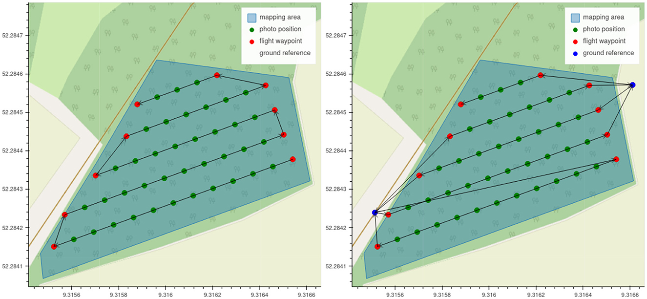
Figure 1. Classical UAV flight path for mapping areas (left) and proposed flight path including reference measurements during flight operation (right). The flight planning tool is freely available. Development and version control is available at https://git.rz.tu-bs.de/m.gerchow/flightplanner, a running instance is accessible online at https://www.isodrones.de/flightplanner/.

2 Materials and methods

2.1 Study area

The study was conducted at a tropical dry forest environment at the Estación Experimental Forestal Horizontes (10°42′46″N 85°35′46″W, 100 m a.s.l.), which is part of the Área de Conservación Guanacaste, located in the northwest of Costa Rica. The site has a mean annual temperature of 25°C and a mean annual precipitation of 1575 mm. The precipitation is highly seasonal, almost all of it occurring between May and November. The UAV flight campaigns were conducted over forest patch of 0.74 ha consisting of evergreen (e.g., Sideroxylon capiri, Swietenia macrophylla) and deciduous tree species (e.g., Guazuma ulmifolia, Astronium graveolens) (Figure 2). Data was collected between May and July 2021 at the end of the dry season and during the transition to the rainy season (Table 1).

Figure 2

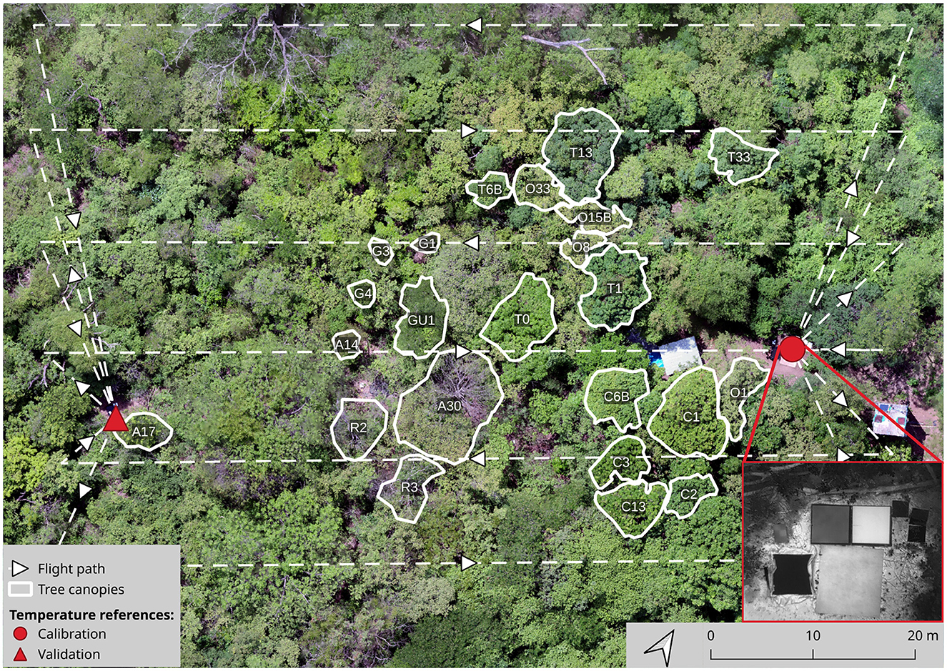
Figure 2. Overview of the study site. The study was conducted at a tropical dry forest in Costa Rica. In order to calibrate and validate the thermal sensor, two locations consisting of temperature ground references were included in the UAV flight plan. The ground references consisted of a black and white painted aluminum sheet and water reference surface (zoomed in rectangle). Twelve of highlighted trees were equipped with sapflow sensor to estimate tree transpiration.

Table 1

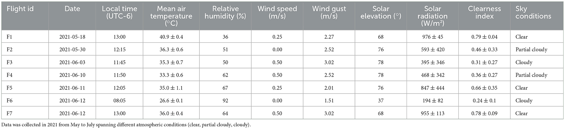
Table 1. UAV flight campaigns and environmental conditions during the flight.

2.2 UAV platform and sensors

The UAV overflights were carried out with a quadcopter (DJI Matrice 210) equipped with a combined visible and thermal camera (Zenmuse XT2). The quadcopter offered a maximum takeoff weight of 6.14 kg, including a payload up to 1.57 kg and a flight time of 38 min (no payload) to 24 min (full payload). The uncooled thermal infrared sensor (microbolometer, longwave infrared spectrum 7.5 to 13 μm) was equipped with a fixed focus lens (focal length 19 mm, field of view 32° × 26°) and offered an image resolution of 640 × 512 pixel. The thermal camera was set to the high gain mode (detectable temperature range from -25°C to 135°C) and the thermal images were saved as radiometric JPEG images (i.e., temperature calibration parameters by the manufacture and raw sensor values were stored within the image metadata). The visible camera (fixed focal length of 8 mm, field of view 57° × 42°) offered an image resolution of 4000 × 3000 pixel. When triggered, the camera captured two individual synchronized images, i.e., a thermal image and a visible image.

2.3 Flight planning

We introduced a novel, alternative flight planning approach in order to increase the number of temperature reference measurements captured in one flight. Multiple measurements are required to achieve a robust temperature calibration and to estimate the temperature drift. We extended current flight planning practices as follows: (1) we repeatedly captured temperature references located at forest clearings during the overflight by integrating the reference locations within the flight plan (Figure 2), (2) the desired image overlap and ground sampling distance is planned at a defined object height (in our case the average tree canopy height) instead of at the ground level, in this way we ensured sufficient image overlap especially at lower flight heights at the canopy level and (3) provide a graphical and user-friendly interface to rapidly plan UAV flights for arbitrary sites.

Mapping areas with UAVs requires a number of sensor parameters (the sensor's image resolution, the size of the image sensor and the focal length) and flight parameters (the area of interest, the flight height, the amount of image overlap in forward and side direction, and the flight speed during image acquisition). The provided sensor and flight parameters are processed into a set of mapping parameters (i.e., the footprint of the aerial image on the ground, the ground sample distance, the distance between photos in forward and side direction, and the time interval between photos) from which the final flight plan (GPS waypoints) is generated (Roth et al., 2018).

We introduced four additional parameters to include reference measurements in the flight plan; (1) the GPS coordinates of the ground temperature references, (2) the speed toward and away from the ground references. Our flight planner determined if a reference measurement is added to the flight plan by (3) limiting the maximum distance allowed to travel to a ground reference and (4) checking the minimum number of images acquired before a reference measurement is repeated. In this way, we avoided introducing excessive flight distances in the case a ground reference is too far away or short flight line cause too many reference measurements. The flight planner¹ generates a list of GPS waypoints, which describe the UAV flight path to capture images for the desired area based on the provided parameters (for this study Table 2). The GPS waypoints were imported into the drone's ground control application (Litchi flight app, VC Technology Ltd, London, England) and executed after stabilizing the thermal camera to ambient temperature for 20 min. Due to a limitation in the drone's waypoint functions (DJI Aircraft firmware 01.02.0450), waypoint actions (e.g., hold position and trigger image acquisition) were not supported when curved turns were enabled. Disabling curved turns increased the total flight time drastically (i.e., a full stop was required for all waypoints) and therefore curved turns were kept enabled, which required to trigger image acquisition at the ground temperature reference waypoints manually by the UAV operator (the flight plan and image acquisition of the overflight area was still executed autonomously).

Table 2

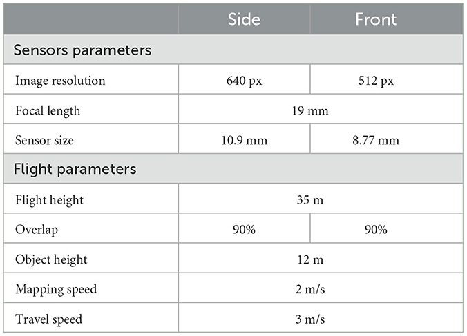
Table 2. Sensor and flight parameters used for the UAV flight planning.

2.4 Ground temperature references

The thermal camera was calibrated and validated against three different types of temperature references. The references reached different temperatures due to different optical absorption coefficients (e.g., white versus black paint). Two thin steel sheets (90 cm × 90 cm × 0.75 mm) were painted in white and black, respectively (All Purpose 2x Flat, Harris Paints, San José, Costa Rica), and insulated with an expanded polystyrene board (100 cm × 100 cm × 5 cm). Prior painting, a thermocouple (Type-T, copper-constantan) was glued to the top side of the steel sheets using thermally conductive glue (SG100X, Silverbead, Bremen, Germany). Two coatings of paint were then applied to ensure that the painted layer was thick enough to be opaque in the long wave infrared spectrum. During midday sun the black reference reached temperatures of > 70°C, which was way above the target temperature (i.e., leaf temperature). Therefore, as a third ground reference, a water surface (1 m × 1 m × 0.3 m) was added. The surface temperature was measured by submerging a thermocouple just below the surface. The reference temperatures were measured (CR1000X Datalogger, Campbell Scientific, Logan, USA) every 10 seconds during the flight. The emissivity of the painted steel sheets was determined by adjusting the emissivity of a hand-held IR thermometer (62 MAX+, FLUKE, Everett, USA) until it reached the temperature measured by the thermocouple.

We used two ground reference sites, the first consisting of three and the second of two ground temperature references, installed in natural forest clearings within the overflight area. The first site was used for calibration and consisted a black, a white and a water surface reference. The second site was used to validate the calibration and consisted of two reference surfaces: A white and a water reference surface (Figure 2).

2.5 Image processing

The acquired thermal and visible images were processed into a geometrically corrected and temperature calibrated orthomosaic. The structure-from-motion (SFM) pipeline was done in a commercial photogrammetry software (Agisoft Metashape 1.8.4) and the temperature calibrations were performed by custom Python scripts. Both images (thermal and visible) were taken simultaneously with a fixed transformation (translation and rotation) between the two sensors. Therefore, the extrinsic parameters (position and orientation) of the thermal images were inferred from the visible images by applying the fixed transformation. After the imagine alignment, ground temperature references were marked in world coordinates and projected into image coordinates. The coordinates were then used to extract the raw radiation values of the ground temperature references from the images.

The image processing steps were as follows:

1. The thermal and visible images were loaded into a multiplane layout (rigid camera rig data, Agisoft, 2023) to infer the extrinsic thermal camera parameters from the visible images.

2. The images were aligned to calibrate the intrinsic parameters, the extrinsic (location and orientation) camera parameters as well as the lens distortion coefficients.

3. The previous alignment resulted in an initial transformation from world coordinates to image coordinates. The alignment was optimized using six ground control points (GCPs). This step also ensured that subsequent orthomosaics created on different flights were aligned.

4. A marker for each temperature reference was added to a thermal image and projected onto the other images. If necessary, the projections were manually adjusted or removed if the temperature reference was not clearly visible in one of the images.

5. The location of each reference for each image was exported to an open standard file format (i.e., LabelMe JSON standard, Russell et al., 2008). From this a dataset consisting of extracted raw surface radiation values from the thermal images and corresponding logged surface temperatures in Celsius was generated.

6. The dataset was used to fit and validate the different temperature calibration methods.

7. A point cloud was generated from the camera calibration step and the point cloud was used to generate a digital elevation model.

8. Before creating the orthomosaic, the original thermal images were replaced with their temperature-calibrated version. The final geometrically referenced and temperature calibrated orthomosaic was exported as GeoTIFF.

The parameters used during image processing are given in the Supplementary Table S1.

2.6 Thermal camera calibration

Five different approaches to calibrate the thermal camera were tested to convert the raw sensor values (stored in the thermal image metadata) to absolute temperature in degree Celsius. As a first step, the dataset was filtered by removing images with a steep viewing angle of the temperature references; a viewing angle of less than 45° is generally recommended to avoid incorrect temperature readings (Nunak et al., 2015). To avoid heterogeneous temperature surfaces, reference surfaces with high standard deviations (>2°C) were also excluded (in some images a temperature reference was partially shaded or occluded and excluded in this way).

We tested two commonly used methods, (1) the camera's factory calibration and (2) the empirical line method (i.e., linear regression between the raw sensor values and logged surface temperatures), as well as three novel methods, which were based on the commonly used methods (3) a modified empirical line method in which the regression is updated each time the set of calibration references was captured (here: repeated empirical line method), (4) a modified factory calibration in which the temperature drift is estimated and corrected (here: factory calibration including drift correction), (5) a second modified empirical line method in which the slope is held constant, and only the intercept was repeatedly updated (here: constant slope repeated empirical line method).

2.6.1 Factory calibration

The factory calibration allowed us to convert the raw sensor values directly into temperatures. A set of manufacture precalibrated parameters were stored in the thermal image metadata, which allowed to convert the raw values to thermal radiation. We used a radiative transfer model to convert the thermal radiation to absolute temperatures (Aubrecht et al., 2016; Tattersall, 2021). In short, the amount of atmospheric absorption depends on the distance between the camera and the subject, the air temperature and the air's relative humidity. Before and after each flight, the reflected ambient temperature was recorded and averaged by measuring a piece of crumpled aluminum foil with the infrared thermometer (emissivity set to 1.0). Atmospheric parameters (air temperature and relative humidity) were logged by a weather station (Hobo RX3000, Onset, Bourne, USA) installed within the forest site. The distance to the subject (i.e., the ground temperature references) was set to the drones flight height (Table 2).

2.6.2 Empirical line method calibration

The raw sensor values from the thermal camera and the logged temperatures from the calibration temperature reference surfaces were used to form a linear regression (Zhou et al., 2005). The linear regression model was fitted once per flight by ordinary least squares and used afterward to convert the raw thermal images to absolute temperatures.

2.6.3 Repeated empirical line method calibration

During the overflight, the temperature surface references were captured after each flight line (Figure 2). Rather than performing the empirical line calibration once per flight, each capture of the calibration temperature reference surfaces was used to fit the linear regression model. The fitted slope and intercept were linearly interpolated in time to convert the thermal images to absolute temperatures.

2.6.4 Factory calibration including drift correction

The raw sensor values from each temperature ground reference were converted to absolute temperatures using the factory calibration. The difference between the converted temperatures and measured reference temperatures was then used to estimate the temperature drift. The difference was linearly interpolated over time and then subtracted from the initial converted temperatures to correct for the temperature drift.

2.6.5 Constant slope repeated empirical line method calibration

We modified the repeated empirical line method to update and interpolate only the intercept. The slope is calibrated once per flight and was assumed to be a constant, i.e., we assumed that the slope was independent of the ambient conditions and regarded as a per sensor value.

2.7 Statistical analysis and comparison of the calibration methods

The accuracy of each calibration was tested against the calibration temperature references (i.e., to determine the goodness of fit of the calibration model, in-sample analysis) and against the data from the validation temperature reference surfaces (i.e., to cross-validate each calibration method, out-sample analysis). In each case, the accuracy of the calibration and validation was determined by the root-mean-square error (RMSE), the mean absolute error (MAE) and the mean difference (MD) for each flight. In addition, the mean temperature difference over the flight time was analyzed to assess the method's robustness against temperature drift.

2.8 Relationships between canopy temperatures and plant water use

In order to further validate the estimated leaf temperatures, we explored the relationships between canopy temperatures and plant water use. Leaf temperatures for the selected tree individuals at one flight date (F1, Figure 3) were extracted using the shape of the canopies, which have been segmented manually using a GIS (Figure 2). We then calculated a temperature histogram for each canopy and determined mean, variance, skew, kurtosis, 5th and 95th percentile of the temperature distributions. 11 of the identified canopies were equipped with sap flow sensors (HPV-06, Implexx Sense, Melbourne, Australia).

Figure 3

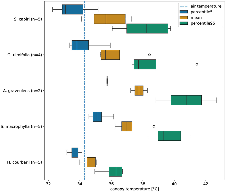
Figure 3. Boxplot of the calculated statistical parameters (5th percentile, mean and 95th percentile) from the whole canopy temperature distribution grouped by each investigated species.

Estimating tree transpiration from sap flow measurements necessitates modeling, particularly when using the heat pulse method, as applied in this study. This method models heat velocity based on convection within the transpirational stream of the trunk. To estimate tree transpiration, heat velocity must be integrated across the conductive sapwood. This procedure is error-prone due to the radial variability in sapwood conductivity, which is challenging to accurately assess, potentially leading to significant errors in transpiration estimates (Gerchow et al., 2023). Information on the processing of the sap flow data can be found in Khnhammer et al. (2023). We extracted total sap flow for the respective hour when the overflight took place [L/h] and the complete data of the overflight [L/day] for each monitored tree. We then performed a correlation analysis of the data from the two temporal representations of sap flow, respectively, and the statistical measures of the calibrated leaf temperatures. Finally, these relationships were evaluated and interpreted in terms of coefficient of determination of the fit, statistical significance and plausibility in terms of water transport and stomatal regulation processes.

3 Results

3.1 Flight planning

The flight plan generated for the study area resulted in seven approaches to the calibration and validation temperature references after each flight line. The average distance between calibration and validation location was 93 m, which took approx. 60 s of flight time (Figure 2). The total flight time was 21 min covering a distance of 1.8 km and an area of 1.1 ha. In comparison, not including temperature ground reference would result in an estimated flight time of 16 min and a distance of 1.4 km (estimations were provided by the ground control app). On average 72 thermal images of the temperature references were acquired per flight, resulting in an average of 180 references measurements (after filtering, 83 measurements were used for the calibration and 33 measurements for the validation).

3.2 Thermal image calibration

The calibration methods exhibited variations in accuracy. The common methods (i.e., factory calibration and empirical line method) overall achieved a lower calibration accuracy compared to the modified methods (i.e., repeated empirical line method, factory calibration including drift correction and constant slope repeated empirical line method). The lowest overall calibration error was obtained using the repeated empirical line method (MAE 0.6°C, Table 3). The commonly used calibration methods produced significantly larger calibration errors (MAE > 2.8°C) when compared to the modified methods where the calibration was updated during the flight (MAE < 1.1°C). The factory camera calibration achieved the lowest calibration error of the common methods (MAE 2.8°C). The common methods showed a large temperature drift during the overflight (MAE of 4.2°C at 5 min after liftoff), which decreased to an MAE of 1.8°C at 12 min after liftoff (Figure 4).

Table 3

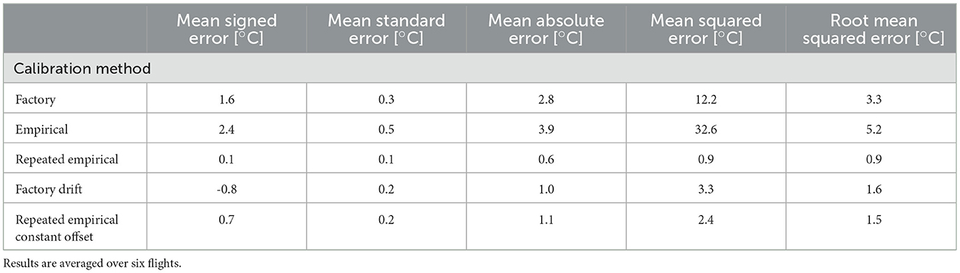
Table 3. Comparison of the accuracy of different calibration methods based on in-sample analysis.

Figure 4

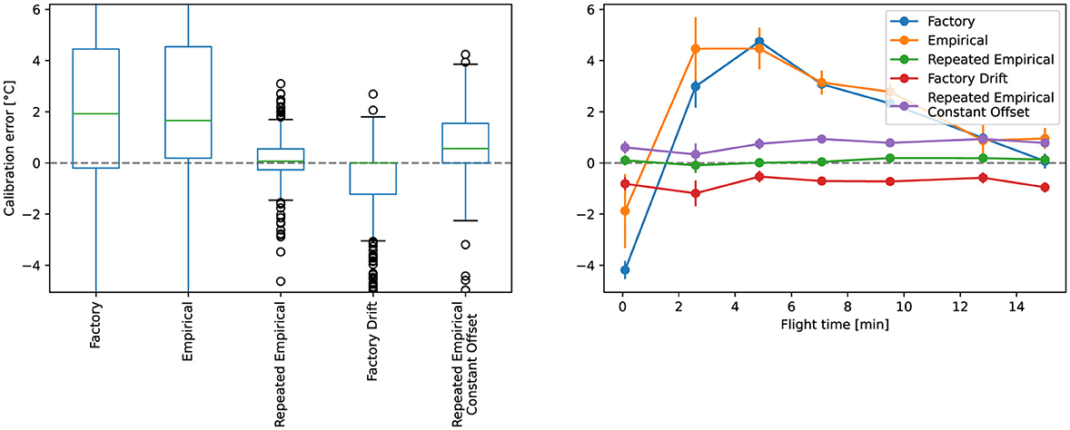
Figure 4. Calibration error averaged over all flights for each calibration methods. Commonly applied method (factory, empirical) result in higher calibration errors and temperature drift compared to proposed approaches (repeated empirical, factory drift, repeated empirical constant offset).

3.3 Validation of the thermal camera calibration

The validation of the calibration methods was done out-sample, i.e., each calibration was cross validated against temperature references not used during calibration. If the calibration was not updated during the overflight we observed significantly larger validation errors (MAE > 3.5°C) compared to the updated methods (MAE < 1.3°C) (Table 4). All calibration techniques showed a temperature drift in the validation result, i.e., the validation error was larger at the beginning of the flight and reduced over time. By applying a repeated calibration method the temperature drift was reduced on average overall flights to a maximum MAE of 2.1°C compared to max. MAE of 5.5°C for the non-repeated calibration approaches (Figure 5). The lowest validation error was achieved by the repeated empirical line method (MAE 1.5°C) and the factory camera calibration including drift correction (MAE 1.6°C) (Table 4).

Table 4

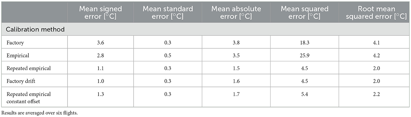
Table 4. Comparison of the accuracy of different calibration methods based on out-sample analysis (cross validation).

Figure 5

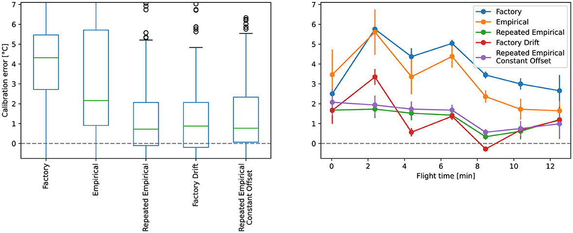
Figure 5. Validation of each applied calibration method. Commonly applied method (factory, empirical) result in higher validation errors and temperature drift when compared to proposed approaches (repeated empirical, factory drift, repeated empirical constant offset).

3.4 Image processing: photogrammetric camera calibration and thermal orthomosaic generation

Image alignment and thermal orthomosaic generation was successful for all flights. On average overall flights, a total of 380,000 tiepoints were detected in 866 images (433 visible images and 433 thermal images), 320,000 tiepoints (740 per image, 86% of total) were used for the photogrammetric calibration of the visible sensor, and 46,000 tiepoints (100 per image, 13% of total) were used for the thermal sensor. An average of 4,600 tiepoints (10 per image, 1% of total) were identified and matched between the two sensors. These tiepoints were used to estimate the rotational transformation (omega, phi, kappa) between the two image coordinate systems of the visible and thermal sensors. The mean and standard deviation averaged over all flights were -1.16 ± 0.30°, 0.84 ± 0.75°, 0.23 ± 0.07°, respectively. The average re-projection error across flights was 1.10 px, while the thermal camera re-projection error was 0.97 px, compared to a re-projection error of 1.23 px of the visible cameras (Table 5). The orthomosaic alignment between the visible and thermal bands was validated by manually matching 10 corresponding points in the visible and thermal bands, the average alignment over all flights was 6.09 ± 3.32 cm (Table 5).

Table 5

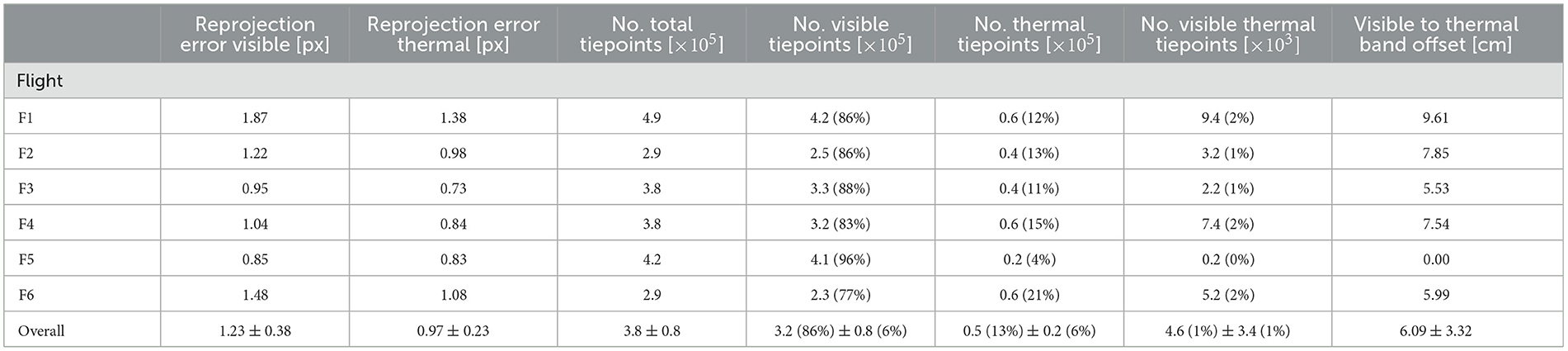
Table 5. Photogrammetric camera calibration results for each flight, including comparisons of the reprojection error, number of image tiepoints, and offset between the visible and thermal sensors.

The effect of the temperature drift is particularly evident in the thermal band generated by the non-updated calibration methods For example, the initial flight lines appear colder and the resulting orthomosaic (e.g., flight F1, Figure 6) shows a temperature gradient perpendicular to the main flight direction. The gradient also resulted in a stretched histogram of the thermal band when compared to the histogram of a calibration method that included a temperature drift correction. Individual leaves are clearly identifiable in the visible band and temperature variations at the leaf scale in the temperature band are detectable (Figure 6).

Figure 6

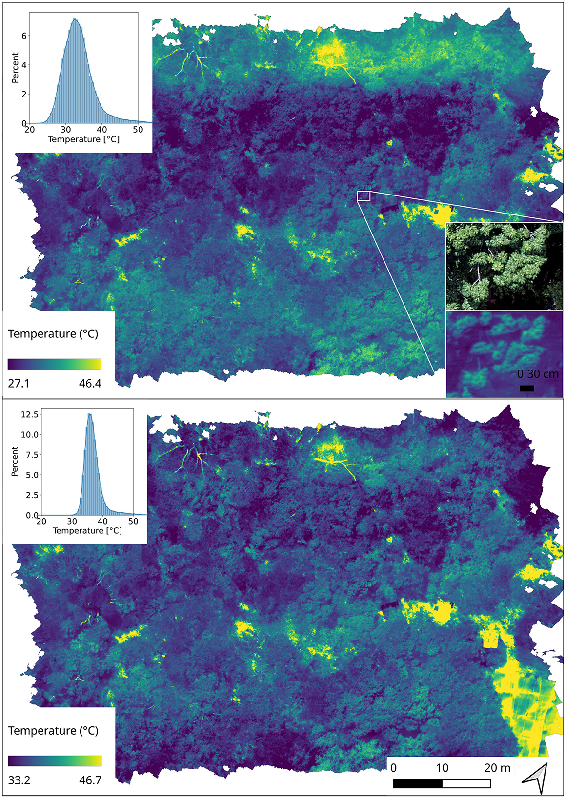
Figure 6. Thermal orthomosaic of the study site at high spatial resolution. Thermal camera temperature drift is visible in the generated orthomosaic (upper orthomosaic revealed a temperature gradient orthogonal to the main flight direction and a stretched histogram). The temperature drift was reduced by the repeated empirical line calibration (no obvious gradient or cold spots in the generated orthomosaic and a narrow histogram).

3.5 Relationship between canopy temperatures and plant water use

For an additional assessment of the derived leaf temperatures, we analyzed the relationships between canopy temperature and sap flow at the time when the UAV overflight took place. Figure 7 shows the results for the highest linear and exponential relationships, respectively, between the leaf temperature statistical measures and sap flow. The linear and exponential fits for all investigated statistical parameters of the leaf canopy temperatures are depicted in Supplementary Figure S1.

Figure 7

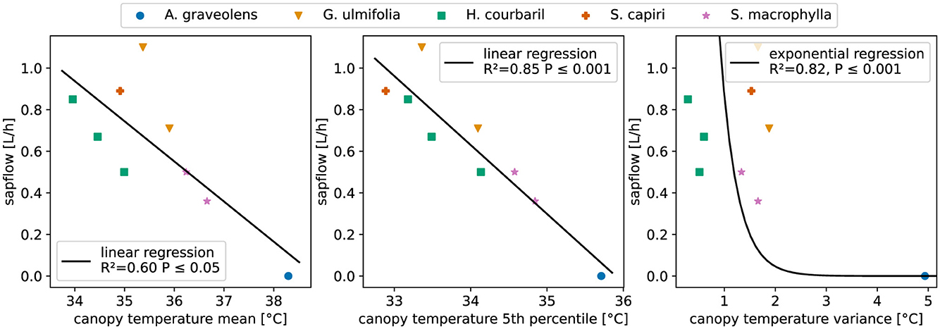
Figure 7. Linear and exponential regression analyses evaluating the relationships between mean canopy temperature, 5th percentile of canopy temperature distribution, and variance of canopy temperature, against sapflow rates.

The correlation analysis reveals that the relationship between canopy temperature and sap flow is generally better represented by an exponential relationship rather than a linear. For the analysis of the linear relationship between statistical parameters of the canopy temperature distributions and sap flow we obtained the highest correlations for the 5th percentile, with a coefficient of determination (R²) of 0.85 (p < 0.001) (Figure 7). This is followed by the mean canopy temperature (R² 0.60, p < 0.05), 95th percentile (R² 0.55, p-value < 0.05) (Supplementary Figure S1). We found no significant linear relationships for the variance, standard deviation, skew and kurtosis of the canopy temperature distribution. The highest R² for the exponential fit is found for the variance of the leaf temperature distributions, reaching an R² as high as 0.82 and a p-value lower than 0.001 (Figure 7, right). Furthermore, std (R² 0.63, p < 0.05) and the 95th percentile (R² 0.71, p < 0.01) of the leaf temperature distributions correlate well with sap flow (Supplementary Figure S1). The relationship of mean canopy temperature and sap flow is still acceptable, reaching an R² of 0.62 and a p-value < 0.05.

4 Discussion

In this study we developed a new flight planning approach to improve UAV-based thermal infrared temperature measurements, in which the locations of temperature ground references are included within the UAV flight planning and are repeatedly captured during the overflight. Especially in dense forest canopies, where a ground reference can only been captured directly from above, this allows for sufficient reference measurements. We tested five different methods to convert the thermal images to absolute temperatures and validated each calibration against the reference measurements. Further, we correlated the absolute temperatures to sapflow measurements of 11 selected trees.

4.1 Thermal image calibration and orthomosaic generation

The new flight-planning approach includes temperature ground references within the UAV flight plan. This enabled us to adjust and validate the UAVs thermal sensor calibration roughly every minute. In contrast, if temperature references are used without being included in the flight plan, they are only captured on fly over, which - depending on the flight path - significantly limits the number of reference measurements. For example, a study conducted over a peatland, where the references were not occluded due to taller objects, resulted in a total of six reference measurements per flight (Kelly et al., 2019). Alternatively, references are captured manually once at the start, on fly over, and before landing resulting in three reference measurements (Gómez-Candón et al., 2016). While our approach increases the number of reference measurements, it also increases the flight time and therefore reduces the maximum coverage of the study site. We applied a simple heuristic to decide when to add reference measurements to the flight path. In the future, a more sophisticated path planning approach using the desired photo positions, constrained by the acquisition of reference measurements and a user-defined spatial or temporal limit, should be implemented into our flight planning approach to minimize the total travel distance and thus reduce the flight time.

We tested five approaches to calibrate the thermal sensor to absolute temperatures. The two commonly used methods (namely, the camera's factory calibration and the empirical line method) suffered from significant temperature drift and proved inaccurate within the initial 12 min (roughly half of the total flight time), with average validated MAE values of 3.8°C and 3.5°C, respectively. The results of the factory calibration are consistent with the findings of Sagan et al. (2019), who reported RMSE values of 3.39°C for the factory calibration. We believe that the inaccuracies are caused by the unstable ambient temperature of the thermal sensor during the initial 12 minutes, as it changes from its initial temperature on the ground to the ambient condition during the flight. In some cases, the thermal images from the first 15 minutes are discarded or extra flight time is added without acquiring thermal images to exclude most of the temperature drift and increase the overall accuracy (Kelly et al., 2019). For our study site, this would effectively halve the useable data. Another approach is to estimate the temperature drift from corresponding pixels matched in sequentially taken thermal images (Mesas-Carrascosa et al., 2018). While this approach potentially reduces the drift, it would still require temperature references to validate absolute temperature measurements. Also, matching corresponding pixels in thermal images remains challenging (Maes et al., 2017) and temperature readings depend on the viewpoint and the respective surface type (Aubrecht et al., 2016), which would affect drift estimations.

By updating the calibration frequently (namely, the repeated empirical line method and factory calibration including drift correction) we are able to reduce the temperature drift. In the repeated empirical line method the calibration parameters are updated with each measurement of the temperature references, which reduced the average validated MAE to 1.5°C and the RMSE to 2.0°C compared to the factory calibration, which resulted in a RMSE of 4.1°C. Alternatively, the thermal sensor can be pre-calibrated against a black body target, achieving a validated in-situ accuracy of 2.6°C (Ribeiro-Gomes et al., 2017). Ideally, the target emissivity must be close to the used reference emissivity to achieve the highest possible accuracy, as a change in emissivity from 0.95 to 0.94 results in roughly a 1°C error (Aubrecht et al., 2016).

As an alternative, we tested a new approach using one temperature reference to estimate the drift of the factory calibration. In the factory calibration including drift correction we achieve the same accuracy as the updated empirical line method calibration, 1.5°C MAE versus 1.6°C MAE. The advantage is that a difference between target and reference emissivity can be included in the temperature calibration. On the other hand, the atmospheric absorption of the target's thermal radiance is modeled, requiring additional environmental parameters and introducing additional uncertainties into the calibration. On the upside, this approach only requires one temperature reference to estimate the temperature drift. In contrast, the empirical methods require at least two references differing in temperature, e.g., a white and a black painted sheet, to create a sufficient temperature span for the line fitting step. The painted temperature references do not generate a temperature span without sufficient solar radiations and therefore can not be used during low irradiance conditions (pre-dawn). As an alternative, more costly actively heated ground references could be used to create a defined stabilized temperature span (Han et al., 2020).

In the case a factory calibration is not available, i.e., the factory calibration normally comes with additional expenses, and only one temperature reference is available, which could already be available in the study site, e.g., snow (Pestana et al., 2019) or a natural water body, that usually provides a stable reference in the time span of the overflight and therefore does not need to be measured continuously. In this scenario, we suggest to use the constant slope repeated empirical line method. In which, the slope (gain) needs to be estimated once in the laboratory, or alternatively in the field against a minimum of two references; afterwards the slope is kept constant as it is independent of the thermal sensors ambient conditions. The one available reference is included using our flight planning approach to repeatedly estimate the intercept (offset). The constant slope updated empirical line method achieves the same accuracy as the factory calibration including drift correction and the updated empirical line method with an MAE value of 1.7°C.

Overall - if available - we recommend using the factory calibration with drift correction as it allows accounting for differences in target and calibration emissivity and can be applied using only once reference. While it requires additional environmental parameters to model radiance absorption, the amount of thermal radiation absorption from the atmosphere at lower flight remains low (Melis et al., 2020) and should not affect the accuracy of the calibration significantly. From our results, we conclude that the biggest challenge to achieve accurate temperature measurements is the estimation and correction of a temperature drift. Therefore, it is crucial that the end user is aware of an occurring temperature drift, which might be less profound in temperate climates, where the change in the ambient condition from the sensor stabilization time on the ground to the ambient condition during the flight might not cause a temperature change of the thermal sensor (Perich et al., 2020). However, if a temperature drift is detected, it needs to be correct to achieve reliable temperature measurements. By using ground reference with a dedicated flight planning we can account for the temperature drift, improve the overall accuracy and validate the temperature calibration.

The thermal images were aligned by transforming their pose from the high resolution visible images, this enabled us to create high resolution thermal orthomosaics of the forest canopies for all flights. While it has been shown that pre aligning thermal images from visible improves their alignment (Maes et al., 2017), we could demonstrate that sufficient tiepoints between the visible and thermal images are detectable to estimate the transformation between the visible and thermal sensor. This allowed us to align both bands in one step, without the need of additional filtering of the thermal images (Ribeiro-Gomes et al., 2017) or an additional alignment step of two independently processed bands (Awais et al., 2022), thereby reducing the overall complexity and processing time during post processing. Although the results of the orthomosaic are satisfactory on a bigger scale (canopy scale) at smaller scales (leaf scale) the thermal and visible bands showed a small spatial offset of 6 cm. The error might be caused by an imperfect synchronization between the two sensors, also suspected in Sledz and Heipke (2022). This result limits the possibility to extract single leaf temperature by identifying leaves within the visible band, nevertheless the identification of single leaves in the temperature band is possible.

4.2 Relationship between canopy temperatures and plant water use

We performed a statistical analysis of the estimated leaf temperatures with the water use of 12 trees at the study site which were equipped with sap flow sensors. We hypothesized that a relationship between the estimated leaf temperatures and sap flow should be observable, following the physical principle that increasing transpiration of water cools plant leaves, all else equal. Since for each tree, the UAV-based high resolution leaf temperature estimates provide a spatially distributed view over the entire canopy, we were able to explore various measures of the entire distribution of temperatures for each canopy, as opposed to one single temperature value for each canopy. This allows for a discussion of both species-specific- and within-tree temperature distributions.

Using the mean temperature value for each canopy resulted in acceptable R² for both the linear and exponential fit (R² of 0.60 and 0.62, respectively and p-values of < 0.05) when correlated against sapflow (Figure 7, Supplementary material S1). However, the leaf temperatures showed substantial variation within their canopy and were highly specific to each tree (Figure 3). The lowest mean leaf temperatures were found for H. courbaril (34.7°C) followed by S.capiri (35.8°C) and G. ulmifolia (36.2°C). Both tree species are evergreens, believed to have access to deep-seated water resources (Hasselquist et al., 2010; Khnhammer et al., 2023). A. graveolens (37.8°C) and S. macrophylla (37.2°C) had the highest mean leaf temperatures. A. graveolens and S. macrophylla are deciduous (or facultative deciduous) tree species, shedding their leaves regularly during the dry season. At the time of the overflights, A. graveolens and some trees of S. macrophylla were starting to shed their leaves and had low measured stomatal conductances (data not shown), indicating decreasing transpiration rates. It is further noted, that for all observed tree species the mean estimated leaf temperatures are greater than recorded air temperature (Figure 3), suggesting little or no transpiration based on the mean canopy temperatures. Indeed, the two species with the highest mean canopy temperatures, A. graveolens and S. macrophylla, also had very low sap flow rates (Figure 7), supporting this notion. In contrast, the 5th percentile of the leaf temperature distributions per species (Figure 3) show that a proportion of leaves of H. courbaril (mean of p5 = 33.7°C), G. ulmifolia (34.2°C) and S. capiri (33.5°C) are clearly below air temperature (Figure 3). For A. graveolens (35.7°C) and S. macrophylla (35.2°C), even the 5th percentile mean temperatures are above air temperature. We interpret this as differences in stomatal traits, i.e., while some species already have most of their stomata closed, others keep certain parts of their canopy transpiring. This is confirmed by the regression analysis presented in Figure 7, where it is shown that canopy temperature correlates best with sap flow when using p5 (R² of 0.85, P < 0.001). The species-specific variability of leaf temperatures also differs between the studied species. H. courbaril has the overall lowest variability of leaf temperatures, with standard deviations of 0.5°C, 0.4°C and 0.7°C for mean canopy temperature, the 5th percentile and the 95th percentile, respectively. This shows that the individual trees of H. courbaril behave relatively similar. In contrast, individual trees of S.capiri (Figure 3) behave differently (std of 1.3°C, 1.2°C and 1.6°C for mean canopy temperature, the 5th percentile and the 95th percentile, respectively). A similar pattern, but less pronounced variability was found for G. ulmifolia, A. graveolens and S. macrophylla. As all trees included in this study have a similar age and all trees within each species have similar size and assuming the derived canopy temperatures are correct, one interpretation might be that S. capiri and G. ulmifolia had different water availability and stomatal regulation traits compared to the other investigated species. In future studies, an extended database (temporally, spatially) of sap flow data vs. leaf temperatures and further plant physiological parameters (e.g., stomatal conductance, leaf water potential) could be used to investigate such species-specific relationships in greater detail.

Looking at within-tree temperature distributions, it can be observed that leaf temperatures are variable not only between individual trees and species (Figure 3) but also within each tree (Figure 8). We try to demonstrate the utility of such individual canopy temperature distribution analysis with the three examples shown in Figure 8, where the temperature distributions for one tree of S. capiri, S. macrophylla and H. courbaril are shown. First, it can be seen here that for all examples, p5 and p95 correspond to the most shaded and most sun-exposed leaves, respectively. The question here is whether the low temperatures observed are caused by transpiration or simply shading. The difficulty here is that in such an extreme climate (i.e., end of the dry season), shaded leaves might be the ones transpiring most. The existence of good correlations between p5 and sap flow might support this relationship. Second, the temperature distributions presented here can facilitate the analysis of the coupling between leaf and air temperatures within a single canopy. These results suggest that an improved understanding of this coupling will be crucial for linking leaf temperature measurements with estimates of transpiration and more generally for understanding tree physiology in the context of global climate.

Figure 8

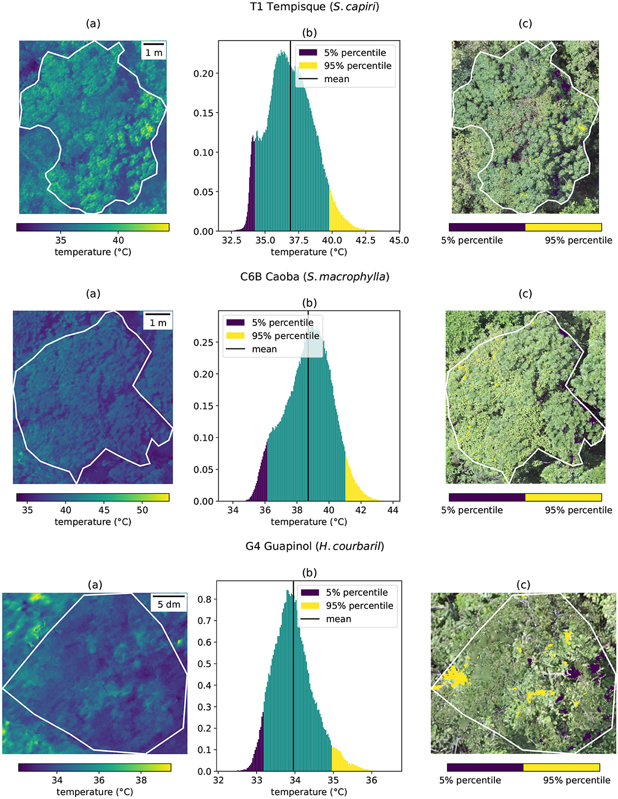
Figure 8. Cropped canopy image extracted from the orthomosaic, generated using calibrated thermal images in absolute temperatures (A). Histogram displaying the distribution of temperature pixels within the delineated canopy (B). Visible light image of the canopy highlighting regions corresponding to the 5th percentile and 95th percentile of the canopy temperature distribution (C). Three examples out of the 21 delineated canopies are shown.

4.3 Outlook

Acquiring absolute temperature with high resolution in mixed-species forest opens up the possibility of single leaf temperature extraction and detailed analysis of canopy temperature distribution. Early stress might affect only parts of the canopy (Pineda et al., 2020), which requires a detailed temperature analysis. In this study, less dense, exposed parts of the canopy reached higher temperatures than densely shaded regions (Figure 8). Many commonly measured tree measurements are carried out at the leaf scale and suffer from several disadvantages: i.) they are strongly affected by the sampling location (e.g., shaded vs sunlit leaves); ii.) it is often difficult to obtain a representative number of replicates; iii.) it is difficult to decide which parts of the canopy are representative for the whole canopy. Hence, such measurements often do not represent the spatial variability of the canopy and fail when upscaled from the measured leaves to the whole canopy. For example, the transpiration of plants is commonly estimated by the Penman-Monteith equation, for which the plant canopy is assumed to be one big leaf. The big leaf assumption, which abstracts the whole canopy into a one-layer source is in conflict with the complex structures of real canopies, where the temperature distribution varies, and consequently influence the canopy transpiration rates. The complexity of real canopies might be better captured by dividing in into sunlit and shaded leaf groups (Luo et al., 2018). High-resolution thermal images enable correlation with local leaf temperatures and might improve scaling to the real canopy.

Data availability statement

The raw data supporting the conclusions of this article will be made available by the authors, without undue reservation.

Author contributions

MG: Writing – original draft, Writing – review & editing. KK: Writing – review & editing. AI: Writing – review & editing. JM: Writing – review & editing. MB: Writing – review & editing.

Funding

The author(s) declare financial support was received for the research, authorship, and/or publication of this article. This research has been supported by the Volkswagen Foundation (contract no. A122505; reference no. 92889).

Conflict of interest

The authors declare that the research was conducted in the absence of any commercial or financial relationships that could be construed as a potential conflict of interest.

Publisher's note

All claims expressed in this article are solely those of the authors and do not necessarily represent those of their affiliated organizations, or those of the publisher, the editors and the reviewers. Any product that may be evaluated in this article, or claim that may be made by its manufacturer, is not guaranteed or endorsed by the publisher.

Supplementary material

The Supplementary Material for this article can be found online at: https://www.frontiersin.org/articles/10.3389/ffgc.2025.1457762/full#supplementary-material

Footnotes

1. ^The flight planning tool is freely available. Development and version control is available at https://git.rz.tu-bs.de/m.gerchow/flightplanner, a running instance is accessible online at https://www.isodrones.de/flightplanner/.

References

Agisoft (2023). Agisoft Metashape User Manual. Version Number: Version 2.0. St. Petersburg:Agisoft LLC.

Google Scholar

Aragon, B., Johansen, K., Parkes, S., Malbeteau, Y., Al-Mashharawi, S., Al-Amoudi, T., et al. (2020). A calibration procedure for field and UAV-based uncooled thermal infrared instruments. Sensors 20:3316. doi: 10.3390/s20113316

PubMed Abstract | Crossref Full Text | Google Scholar

Aubrecht, D. M., Helliker, B. R., Goulden, M. L., Roberts, D. A., Still, C. J., and Richardson, A. D. (2016). Continuous, long-term, high-frequency thermal imaging of vegetation: Uncertainties and recommended best practices. Agricult. Forest Meteorol. 228–229, 315–326. doi: 10.1016/j.agrformet.2016.07.017

Crossref Full Text | Google Scholar

Awais, M., Li, W., Cheema, M. J. M., Hussain, S., Shaheen, A., Aslam, B., et al. (2022). Assessment of optimal flying height and timing using high-resolution unmanned aerial vehicle images in precision agriculture. Int. J. Environm. Sci. Technol. 19, 2703–2720. doi: 10.1007/s13762-021-03195-4

Crossref Full Text | Google Scholar

Beyer, M., Iraheta, A., Gerchow, M., Kuehnhammer, K., Callau-Beyer, A. C., Koeniger, P., et al. (2025). UAV-based land surface temperatures and vegetation indices explain and predict spatial patterns of soil water isotopes in a tropical dry forest. Water Resour. Res. 61:e2024WR037294. doi: 10.1029/2024WR037294

Crossref Full Text | Google Scholar

Bulusu, M., Ellser, F., Stiegler, C., Ahongshangbam, J., Marques, I., Hendrayanto, H., et al. (2023). UAV-based thermography reveals spatial and temporal variability of evapotranspiration from a tropical rainforest. Front. Forests Global Change 6:1232410. doi: 10.3389/ffgc.2023.1232410

Crossref Full Text | Google Scholar

Easterday, K., Kislik, C., Dawson, T., Hogan, S., and Kelly, M. (2019). Remotely Sensed Water Limitation in Vegetation: Insights from an Experiment with Unmanned Aerial Vehicles (UAVs). Remote Sensing 11(16):1853. doi: 10.3390/rs11161853

Crossref Full Text | Google Scholar

Ecke, S., Dempewolf, J., Frey, J., Schwaller, A., Endres, E., Klemmt, H.-J., et al. (2022). UAV-based forest health monitoring: a systematic review. Remote Sens. 14:3205. doi: 10.3390/rs14133205

Crossref Full Text | Google Scholar

Ellser, F., Rll, A., Stiegler, C., Hendrayanto, and Hlscher, D. (2020). Introducing QWaterModel, a QGIS plugin for predicting evapotranspiration from land surface temperatures. Environm. Model. Softw. 130:104739. doi: 10.1016/j.envsoft.2020.104739

Crossref Full Text | Google Scholar

Farella, M. M., Fisher, J. B., Jiao, W., Key, K. B., and Barnes, M. L. (2022). Thermal remote sensing for plant ecology from leaf to globe. J. Ecol. 110, 1996–2014. doi: 10.1111/1365-2745.13957

Crossref Full Text | Google Scholar

Gago, J., Douthe, C., Coopman, R., Gallego, P., Ribas-Carbo, M., Flexas, J., et al. (2015). UAVs challenge to assess water stress for sustainable agriculture. Agricult. Water Managem. 153, 9–19. doi: 10.1016/j.agwat.2015.01.020

Crossref Full Text | Google Scholar

Gerchow, M., Marshall, J. D., Khnhammer, K., Dubbert, M., and Beyer, M. (2023). Thermal imaging of increment cores: a new method to estimate sapwood depth in trees. Trees 37, 349–359. doi: 10.1007/s00468-022-02352-7

Crossref Full Text | Google Scholar

Gómez-Candón, D., Virlet, N., Labb, S., Jolivot, A., and Regnard, J.-L. (2016). Field phenotyping of water stress at tree scale by UAV-sensed imagery: new insights for thermal acquisition and calibration. Preci. Agricult. 17, 786–800. doi: 10.1007/s11119-016-9449-6

Crossref Full Text | Google Scholar

Han, X., Thomasson, J. A., Swaminathan, V., Wang, T., Siegfried, J., Raman, R., et al. (2020). Field-based calibration of unmanned aerial vehicle thermal infrared imagery with temperature-controlled references. Sensors 20:7098. doi: 10.3390/s20247098

PubMed Abstract | Crossref Full Text | Google Scholar

Hartmann, W., Tilch, S., Eisenbeiss, H., and Schindler, K. (2012). Determination of the UAV position by automatic processing of thermal images. Int. Arch. Photogramm. Remote Sens. Spat. Inform. Sci. 39, 111–116. doi: 10.5194/isprsarchives-XXXIX-B6-111-2012

Crossref Full Text | Google Scholar

Hasselquist, N. J., Allen, M. F., and Santiago, L. S. (2010). Water relations of evergreen and drought-deciduous trees along a seasonally dry tropical forest chronosequence. Oecologia 164, 881–890. doi: 10.1007/s00442-010-1725-y

PubMed Abstract | Crossref Full Text | Google Scholar

Kelly, J., Kljun, N., Olsson, P.-O., Mihai, L., Liljeblad, B., Weslien, P., et al. (2019). Challenges and best practices for deriving temperature data from an uncalibrated UAV thermal infrared camera. Remote Sensing 11:567. doi: 10.3390/rs11050567

Crossref Full Text | Google Scholar

Khnhammer, K., van Haren, J., Kbert, A., Bailey, K., Dubbert, M., Hu, J., et al. (2023). Deep roots mitigate drought impacts on tropical trees despite limited quantitative contribution to transpiration. Sci. Total Environm. 893:164763. doi: 10.1016/j.scitotenv.2023.164763

PubMed Abstract | Crossref Full Text | Google Scholar

Kim, Y., Still, C. J., Hanson, C. V., Kwon, H., Greer, B. T., and Law, B. E. (2016). Canopy skin temperature variations in relation to climate, soil temperature, and carbon flux at a ponderosa pine forest in central Oregon. Agricult. Forest Meteorol. 226–227, 161–173. doi: 10.1016/j.agrformet.2016.06.001

Crossref Full Text | Google Scholar

Lawson, T., and Blatt, M. R. (2014). Stomatal size, speed, and responsiveness impact on photosynthesis and water use efficiency. Plant Physiol. 164, 1556–1570. doi: 10.1104/pp.114.237107

PubMed Abstract | Crossref Full Text | Google Scholar

Leuzinger, S., and Krner, C. (2007). Tree species diversity affects canopy leaf temperatures in a mature temperate forest. Agricult. Forest Meteorol. 146, 29–37. doi: 10.1016/j.agrformet.2007.05.007

Crossref Full Text | Google Scholar

Leuzinger, S., Vogt, R., and Krner, C. (2010). Tree surface temperature in an urban environment. Agricult. Forest Meteorol. 150, 56–62. doi: 10.1016/j.agrformet.2009.08.006

Crossref Full Text | Google Scholar

Luo, X., Chen, J. M., Liu, J., Black, T. A., Croft, H., Staebler, R., et al. (2018). Comparison of big-leaf, two-big-leaf, and two-leaf upscaling schemes for evapotranspiration estimation using coupled carbon-water modeling. J. Geophys. Res.: Biogeosci. 123, 207–225. doi: 10.1002/2017JG003978

Crossref Full Text | Google Scholar

Maes, W., Huete, A., Avino, M., Boer, M., Dehaan, R., Pendall, E., et al. (2018). Can UAV-based infrared thermography be used to study plant-parasite interactions between mistletoe and eucalypt trees? Remote Sensing 10:2062. doi: 10.3390/rs10122062

Crossref Full Text | Google Scholar

Maes, W. H., Huete, A. R., and Steppe, K. (2017). Optimizing the processing of UAV-based thermal imagery. Remote Sens. 9:476. doi: 10.3390/rs9050476

PubMed Abstract | Crossref Full Text | Google Scholar

Marzahn, P., Flade, L., and Sanchez-Azofeifa, A. (2020). Spatial estimation of the latent heat flux in a tropical dry forest by using unmanned aerial vehicles. Forests 11:604. doi: 10.3390/f11060604

Crossref Full Text | Google Scholar

McDowell, N., Pockman, W. T., Allen, C. D., Breshears, D. D., Cobb, N., Kolb, T., et al. (2008). Mechanisms of plant survival and mortality during drought: why do some plants survive while others succumb to drought? New Phytol. 178, 719–739. doi: 10.1111/j.1469-8137.2008.02436.x

PubMed Abstract | Crossref Full Text | Google Scholar

Melis, M., Da Pelo, S., Erb, I., Loche, M., Deiana, G., Demurtas, V., et al. (2020). Thermal remote sensing from UAVs: a review on methods in coastal cliffs prone to landslides. Remote Sens. 12:1971. doi: 10.3390/rs12121971

Crossref Full Text | Google Scholar

Mesas-Carrascosa, F.-J., Prez-Porras, F., Meroo de Larriva, J. E., Mena Frau, C., Agera-Vega, F., Carvajal-Ramrez, F., et al. (2018). Drift correction of lightweight microbolometer thermal sensors on-board unmanned aerial vehicles. Remote Sens. 10:615. doi: 10.3390/rs10040615

Crossref Full Text | Google Scholar

Niu, H., Hollenbeck, D., Zhao, T., Wang, D., and Chen, Y. (2020). Evapotranspiration estimation with small UAVs in precision agriculture. Sensors 20:6427. doi: 10.3390/s20226427

PubMed Abstract | Crossref Full Text | Google Scholar

Novick, K. A., and Katul, G. G. (2020). The duality of reforestation impacts on surface and air temperature. J. Geophysical Res.: Biogeosci. 125:e2019JG005543. doi: 10.1029/2019JG005543

Crossref Full Text | Google Scholar

Nunak, T., Rakrueangdet, K., Nunak, N., and Suesut, T. (2015). Thermal image resolution on angular emissivity measurements using infrared thermography. Lect. Notes Eng. Comp. Sci. 1, 323–327.

Google Scholar

Perich, G., Hund, A., Anderegg, J., Roth, L., Boer, M. P., Walter, A., et al. (2020). Assessment of multi-image unmanned aerial vehicle based high-throughput field phenotyping of canopy temperature. Front. Plant Sci. 11:150. doi: 10.3389/fpls.2020.00150

PubMed Abstract | Crossref Full Text | Google Scholar

Pestana, S., Chickadel, C. C., Harpold, A., Kostadinov, T. S., Pai, H., Tyler, S., et al. (2019). Bias correction of airborne thermal infrared observations over forests using melting snow. Water Resour. Res. 55, 11331–11343. doi: 10.1029/2019WR025699

Crossref Full Text | Google Scholar

Pineda, M., Barn, M., and Prez-Bueno, M.-L. (2020). Thermal imaging for plant stress detection and phenotyping. Remote Sens. 13:68. doi: 10.3390/rs13010068

Crossref Full Text | Google Scholar

Ribeiro-Gomes, K., Hernndez-Lpez, D., Ortega, J., Ballesteros, R., Poblete, T., and Moreno, M. (2017). Uncooled thermal camera calibration and optimization of the photogrammetry process for UAV applications in agriculture. Sensors 17:2173. doi: 10.3390/s17102173

PubMed Abstract | Crossref Full Text | Google Scholar

Roth, L., Hund, A., and Aasen, H. (2018). PhenoFly planning tool: flight planning for high-resolution optical remote sensing with unmanned areal systems. Plant Methods 14, 1–21. doi: 10.1186/s13007-018-0376-6

PubMed Abstract | Crossref Full Text | Google Scholar

Russell, B. C., Torralba, A., Murphy, K. P., and Freeman, W. T. (2008). LabelMe: a database and web-based tool for image annotation. Int. J. Comput. Vis. 77, 157–173. doi: 10.1007/s11263-007-0090-8

Crossref Full Text | Google Scholar

Sagan, V., Maimaitijiang, M., Sidike, P., Eblimit, K., Peterson, K. T., Hartling, S., et al. (2019). UAV-based high resolution thermal imaging for vegetation monitoring, and plant phenotyping using ICI 8640 P, FLIR Vue Pro R 640, and thermoMap cameras. Remote Sens. 11:330. doi: 10.3390/rs11030330

Crossref Full Text | Google Scholar

Santesteban, L., Di Gennaro, S., Herrero-Langreo, A., Miranda, C., Royo, J., and Matese, A. (2017). High-resolution UAV-based thermal imaging to estimate the instantaneous and seasonal variability of plant water status within a vineyard. Agricult. Water Managem. 183, 49–59. doi: 10.1016/j.agwat.2016.08.026

Crossref Full Text | Google Scholar

Sledz, A., and Heipke, C. (2022). Joint bundle adjustment of thermal infra-red and optical images based on multimodal matching. Int. Arch. Photogramm. Remote Sens. Spat. Inform. Sci. XLIII-B1-2022, 157–165. doi: 10.5194/isprs-archives-XLIII-B1-2022-157-2022

Crossref Full Text | Google Scholar

Smigaj, M., Gaulton, R., Barr, S. L., and Surez, J. C. (2015). UAV-borne thermal imaging for forest health monitoring: detection of disease-induced canopy temperature increase. Int. Arch. Photogramm. Remote Sens. Spat. Inform. Sci. XL-3/W3, 349–354. doi: 10.5194/isprsarchives-XL-3-W3-349-2015

Crossref Full Text | Google Scholar

Tattersall, G. (2021). gtatters/Thermimage: Thermimage v4.1.3. doi: 10.5281/zenodo.1069704

Crossref Full Text | Google Scholar

Torres-Rua, A. (2017). Vicarious calibration of sUAS microbolometer temperature imagery for estimation of radiometric land surface temperature. Sensors 17:1499. doi: 10.3390/s17071499

PubMed Abstract | Crossref Full Text | Google Scholar

Yi, K., Smith, J. W., Jablonski, A. D., Tatham, E. A., Scanlon, T. M., Lerdau, M. T., et al. (2020). High heterogeneity in canopy temperature among co-occurring tree species in a temperate forest. J. Geophys. Res.: Biogeosci. 125:e2020JG005892. doi: 10.1029/2020JG005892

Crossref Full Text | Google Scholar

Zhang, J., Huang, Y., Pu, R., Gonzalez-Moreno, P., Yuan, L., Wu, K., et al. (2019). Monitoring plant diseases and pests through remote sensing technology: a review. Comp. Electron. Agricult. 165:104943. doi: 10.1016/j.compag.2019.104943

Crossref Full Text | Google Scholar

Zhou, H.-x., Lai, R., Liu, S.-q., and Jiang, G. (2005). New improved nonuniformity correction for infrared focal plane arrays. Opt. Commun. 245, 49–53. doi: 10.1016/j.optcom.2004.09.077

PubMed Abstract | Crossref Full Text | Google Scholar