 Lina Ke1,2
 Yao Lu
 Qin Tan
- 1School of Geographical Sciences, Liaoning Normal University, Dalian, China
- 2Institute of Marine Sustainable Development, Liaoning Normal University, Dalian, China
- 3National Marine Environmental Monitoring Center, Dalian, China
Mapping coastal wetlands' spatial distribution and spatiotemporal dynamics is crucial for ecological conservation and restoration efforts. However, the high hydrological dynamics and steep environmental gradients pose challenges for precise mapping. This study developed a new method for mapping coastal wetlands using time-series remote sensing images and a deep learning model. Precise mapping and change analysis were conducted in the Liaohe Estuary Reserve in 2017 and 2022. The results demonstrated the superiority of Temporal Optimize Features (TOFs) in feature importance and classification accuracy. Incorporating TOFs into the ResNet model effectively combined temporal and spatial information, enhancing coastal wetland mapping accuracy. Comparative analysis revealed ecological restoration trends, emphasizing artificial restoration's predominant role in salt marsh vegetation rehabilitation. These findings provide essential technical support for coastal wetland ecosystem monitoring and contribute to the study of sustainability under global climate change.
1 Introduction
Coastal wetlands are the transition zone between terrestrial and marine ecosystems, providing essential ecosystem services and material productivity critical to human life and economic activities (National Research Council, 1995). Coastal wetland ecosystems face accelerated degradation and disappearance due to global climate change, rising sea levels, urban expansion, and population growth (Mao et al., 2018a,b; Ren et al., 2019; Li et al., 2022). Over 50% of global wetlands have disappeared since the 18th century, and China's coastal wetlands are also facing severe threats (Wang et al., 2012; Ma et al., 2014; Xu et al., 2019). Therefore, acquiring accurate and real-time data on the spatial distribution of coastal wetlands is crucial for optimizing ecosystem management and achieving sustainable development goals.
Remote sensing technology, with its advantages of wide observation range, extensive data acquisition, and robust data comparability, has been widely used in coastal wetland resource surveys, ecological monitoring, and ecosystem service assessment (Liu et al., 2017). Reviewing 50 years of research in wetland remote sensing, Mao et al. (2023) concluded that despite diverse trends in the field, the accurate extraction and mapping of wetland distribution remains a critical theme of wetland remote sensing research. Multi-scale wetland mapping researches continuously released and updated in recent years provide strong support for this view (Gong et al., 2010; Niu et al., 2012; Murray et al., 2019; Zhang et al., 2022; Wang M. et al., 2023).
However, the precise mapping of coastal wetlands remains an essential challenge. Hydrological dynamics and environmental gradient fluctuations make wetlands one of the most challenging land cover categories to classify accurately in global datasets (Gong et al., 2016). Frequent changes in hydrological conditions create highly dynamic wetland environments throughout the year and seasons, leading to pronounced spectral variations. These variations cause rapid transitions in vegetation communities within short distances in the transition zones between land and sea. For instance, species such as Phragmites australis (P. australis) and Suaeda salsa (S. salsa) can quickly alternate within steep environmental gradients, resulting in spectral confusion among different vegetation types and posing the challenges of classification and mapping.
Time-series remote sensing analysis combined with deep learning techniques provides a solution for precise coastal wetland mapping. Time-series images offer ample phenological information about wetland vegetation, essential for enhancing classification accuracy (Zhu and Woodcock, 2014; Kovács et al., 2022). Feature extraction from time-series images generally involves phenological feature extraction and time-series composite methods (Zhang et al., 2024). Phenological feature extraction typically employs filtering or curve-fitting techniques to reconstruct vegetation indices, capturing essential phenological information (Verbesselt et al., 2010; Cai et al., 2017). Techniques such as thresholding, curve-based analysis, and mathematical methods are commonly used (Liu and Li, 2021; Sun et al., 2021). This method is sensitive to the spatiotemporal resolution of the imagery, and the choice of reconstruction and extraction methods can significantly impact the accuracy of the extracted phenological features (Xiang et al., 2018; Xie and Zhang, 2023). Time-series composite methods aggregate remote sensing images over a defined period and use statistical techniques, such as maximum, mean, and median, to extract land cover features from the images (Ni et al., 2021; Wang Y. et al., 2023). This method may reduce the data size in the temporal dimension and extract essential features of typical wetland vegetation. However, the choice of time scale critically impacts the composite results (Wu and Wu, 2023). Extended time scales may lead to the loss of critical information, affecting wetland vegetation classification accuracy. In contrast, short time scales may increase the complexity of data processing. Consequently, refining existing time-series feature extraction methods and identifying key temporal phases (KTPs) are essential for precise wetland classification (Henderson and Lewis, 2008).
Deep learning models, with their robust capabilities in managing high-dimensional and complex data sets, show promising applications in coastal wetland mapping (O'Neil et al., 2020; Cheng et al., 2023). Several architectures, including Convolutional Neural Networks (CNNs), Generative Adversarial Networks (GANs), U-Net, DeepNet, and Transformers, have achieved impressive outcomes in wetland remote sensing mapping (Ludwig et al., 2019; Jamali et al., 2021a,b; Li et al., 2021; Zhang W. et al., 2023). Mahdianpari et al. (2020) reported that CNN-based methods achieved the highest accuracy compared to other classification algorithms, followed by the random forest (RF) model. However, the superiority of deep learning methods is not absolute. Research by Heydari and Mountrakis (2018) demonstrated that the standard machine learning methods outperformed deep learning in land cover classification using Landsat images. In addition, the extensive need for annotated data and computational resources also limits practical deep learning (Günen, 2022). Therefore, further research and assessment are needed to confirm the accuracy and effectiveness of machine learning and deep learning in coastal wetlands mapping.
As the northernmost estuarine wetland in China, the Liaohe Estuary wetland preserves a typical and intact temperate coastal wetland ecosystem and estuarine landscape. Wetland vegetation, represented by S. salsa and P. australis communities, is widely distributed here, serving as a typical example of a secondary succession of plant communities in the northern plains of China's rivers. To decrease the impact of human activities on the ecosystem, the Liaohe Estuary Reserve (simply “LER” for short) has implemented strict restriction management and ecological restoration projects in recent years. It has also been incorporated into the national park creation zone, making the LER an ideal area for precisely mapping coastal wetlands and assessing ecological restoration effects.
This paper aims to develop a coastal wetland mapping method based on time-series remote sensing imagery and a deep learning model, using the LER as a case study to verify its effectiveness. The main contributions of this paper include (1) developing a new method for temporal feature extraction and highlighting the importance of selecting KTPs and optimized features to improve classification accuracy; (2) combining Temporal Optimize Features (TOFs) with Residual Neural Networks (ResNet) to further enhance wetland classification accuracy; and (3) revealing the ecological restoration effects within the LER from 2017 to 2022 and identifying the primary sources of these restoration effects. The results provide technical support for precise monitoring of coastal wetland ecosystems, offer reference data for evaluating ecological restoration effectiveness, and are essential for managing and conserving coastal wetlands.
2 Study area and data
2.1 Study area
The LER is located in the southern region of Panjin City, Liaoning Province, China (121°28′24.58″-121°45′27.49″ E, 40°45′00″-41°05′54.13″ N), with a total area of about 120,000 hectares (Figure 1). The wetland is formed by the deposition of the Liao River, Daling River, Xiaoling River, and other rivers, mainly mudflats, with flat and open terrain and <7 meters above sea level. The average annual temperature in the study area is 8.5°C, and the average annual rainfall is 650 mm. Natural wetlands include various types, such as tidal flats, salt marshes, and shallow marine siltation. S. salsa and P. australis are two typical salt marsh vegetation types. In response to the increasing effects of climate change and human activities on coastal wetlands, the reserve manager adopted a series of conservation projects, such as “retreating to wetland”. Additionally, the reserve began enforcing prohibition management measures in 2017 to mitigate the impacts of human activities on the ecological environment. In this context, the study focused on LER in 2017 and 2022 to verify the applicability of the mapping method and to reveal the ecological restoration effect of the reserve since its prohibition. The results of this study can provide essential information and a basis for decision-making in managing the reserve's ecosystem.
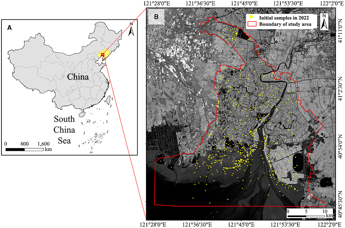
Figure 1. The location of the study area. (A) China, (B) Near-infrared (NIR) band of Sentinel-2 MSI.
2.2 Wetland classification system
This study classified the land cover types in the study area into six primary categories: S. salsa, P. australis, paddy, water, tidal flat, and impervious, based on field surveys of the study area and referencing current classification standards and existing research (Wen et al., 2011; Tan et al., 2022). These primary categories were identified using remote sensing interpretation methods. To distinguish between artificial and natural surfaces and reveal the effects of artificial restoration and natural restoration, this study further subdivided the water category into four secondary categories through visual interpretation: inland water, coastal water, aquaculture, and reservoir. The wetland classification system and its details are shown in Table 1.
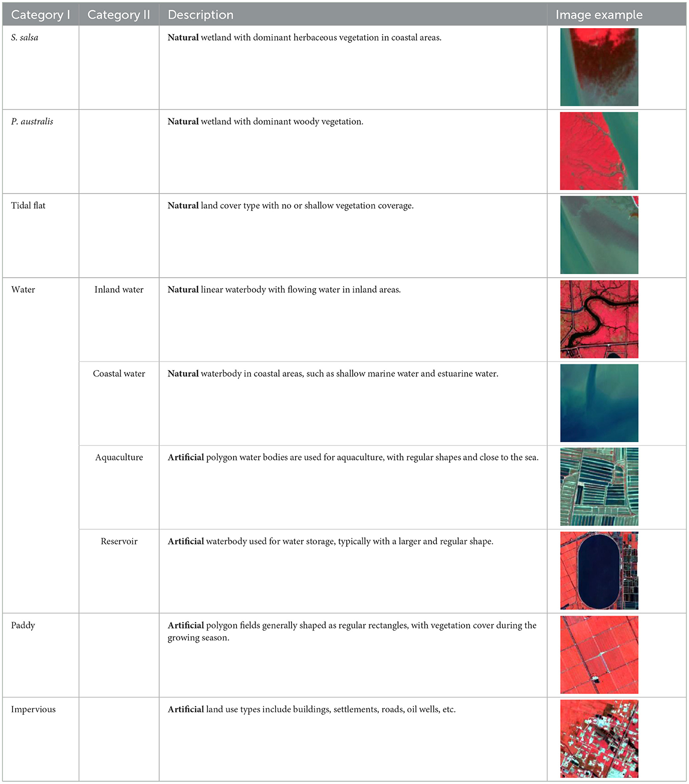
Table 1. Wetland classification system in this study.
2.3 Sample data
This study collected 1,400 initial samples, with 300 from 2017 and 1,100 from 2022. The 300 samples obtained in 2017 were based on visual interpretation of remote sensing imagery. To ensure the spatial distribution and class balance, 50 samples were uniformly selected for each land category, totaling 300. The 1,100 samples for the year 2022 were obtained through field surveys and visual interpretation. The field survey was conducted on September 28, 2022, using handheld geographic positioning systems and unmanned aerial vehicles, collecting 387 field samples. Visual interpretation of Google Earth imagery was used to supplement the data due to the concentrated distribution of the points and ensure a uniform sample distribution in the study area. All initial samples were used to construct TOFs and assess the importance of features.
To obtain sufficient samples for comprehensive training of the deep learning model, this study expanded the initial samples by referring to the method described by Wang M. et al. (2023). Specifically, the study area's remote sensing images were pre-classified using the initial samples and the RF algorithm. The classification results were then converted into vector data for manual review and modification, obtaining different land class vector patches within the study area. Based on the spatial extent of the vector patches, 3,000 samples were randomly generated for each land class, ensuring the balance and representativeness of the sample data during the training of the deep learning model. All initial and expanded sample points were merged and divided into training and validation samples at a 7:3 ratio. These samples were used to train and validate the ResNet and RF models based on different feature combinations.
2.4 Data preprocess
A total of 400 available Sentinel-2 images were obtained in this study based on the Google Earth Engine (GEE) platform, including 298 in 2022 and 102 in 2017. All images were filtered based on a cloud content of <30%, followed by cloud masking using quality assessment bands. Finally, mosaicking and clipping were performed on images with the same imaging dates, resulting in time-series image stacks for the study area of 2017 and 2022. The 2017 time-series image stack included 37 high-quality observations, while 2022 included 67 high-quality observations.
3 Methods
Figure 2 illustrates the research framework of this study. Initially, conventional single temporal features (STFs) were constructed using available images close to the field survey date, including spectral reflectance, vegetation indices, and water indices. Subsequently, TOFs were extracted by applying NDVI time-series reconstruction and Jeffries-Matusita (J-M) feature distance algorithms to time-series remote sensing images, supplementing the STFs with temporal information. To test the effectiveness of the TOFs, monthly composite features (MCFs) were extracted from time-series remote sensing imagery using the monthly average composite algorithm as a control experiment. The importance of different features was examined using the RF algorithm, and the enhancement effects of the two types of temporal features on model classification accuracy were compared. Finally, by post-processing the results of the RF model, an equal number and evenly distributed set of samples were produced, enabling the training, accuracy validation, and classification mapping of the ResNet model.
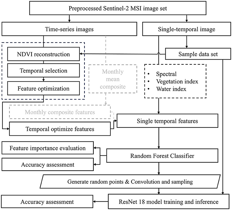
Figure 2. The research framework of this study. Dashed lines represent the control experimental group using monthly mean composite features.
3.1 TOFs extraction
3.1.1 Identification of KTPs
Seasonal and periodic variations in the spectral reflectance of vegetation during the year resulted in evident differences in the separability of land cover type samples at different temporal phases (Wang et al., 2024). Figure 3 displays histograms representing the frequency distribution of normalized vegetation indices (NDVI) for samples of S. salsa, P. australis, paddy, and tidal flats. The separation and overlap between the different categories along the horizontal axis indicate the separability between the land cover samples. As shown in Figure 3, vegetation land classes are mostly indistinguishable throughout the year, with better separability observed in July, August, and September. Therefore, selecting KTPs for classification from time-series remote sensing images is essential for improving the classification accuracy of vegetation communities.
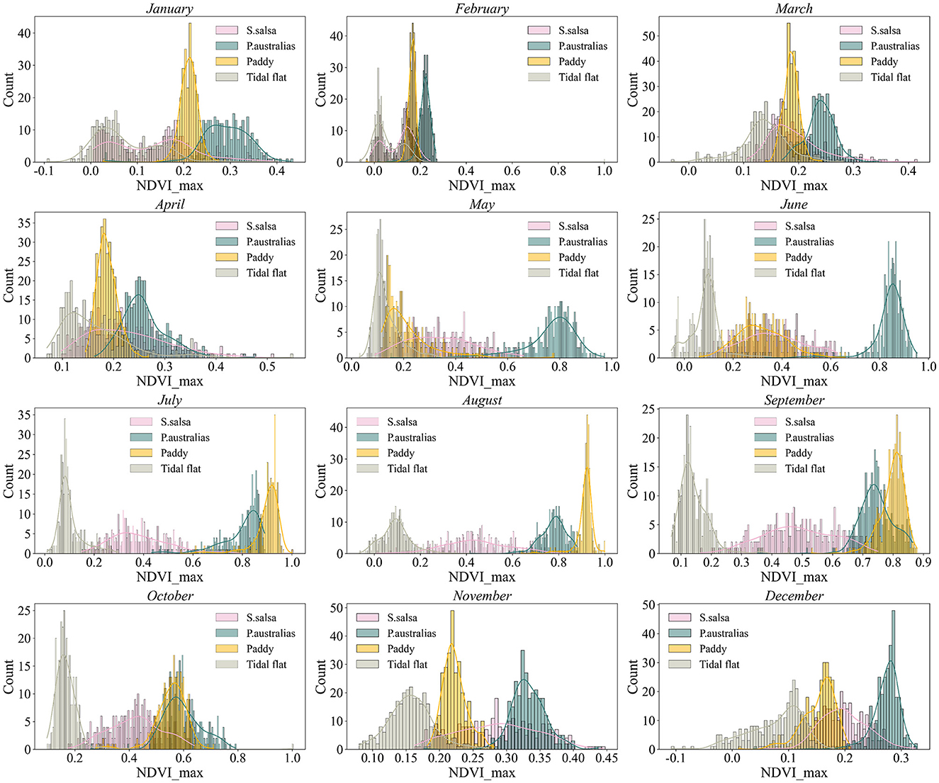
Figure 3. Variations in sample separability across different months within the year. The statistical distribution map of sample is based on sampling from the monthly maximum composited NDVI feature map.
To capture the phenological changes in coastal wetlands, researchers have filtered or fitted time-series vegetation indices due to apparent annual variations in the growth state of salt marsh vegetation (Liu and Li, 2021). This study employed the Savitzky-Golay (S-G) filtering method for the time-series reconstruction of NDVI. The spatiotemporal scale of the data does not limit this algorithm and can capture local information anomalies, effectively removing noise from the time-series data (Schafer, 2011). The expression is shown as follows in Formula (1) (Wu and Wu, 2023).
Where j is the index value in the original NDVI value, is the filtered time-series data value, Yj+i is the original time-series data value, Ci is the filter coefficient of the i-th NDVI value, obtained through least squares polynomial fitting; and m denotes the sliding window broadband (2* m +1). After several adjustments, when m =5 and the polynomial fitting order was set to 3, an ideal fitting effect on the NDVI time-series data was achieved. Thus, the difference between any two types of land classes in the time-series curve was used to determine the KTPs for the complete phenology period, as shown in Figure 4.

Figure 4. NDVI temporal reconstruction curve. The scatter points represent the average NDVI true values of the sample, while the curve represents the temporal growth curve obtained after S-G filtering and fitting. The dashed line indicates the determined KTPs.
3.1.2 Spectral separability evaluation
The J-M distance is a widely recognized measure of spectral separability (Ni et al., 2021), providing a quantitative metric for measuring the separation between two or more categories in feature space, and has been extensively applied in remote sensing image classification and feature optimization. This study calculated the J-M distance based on the Bhattacharyya distance between samples to determine the features at each KTPs. The expression is as follows in Formulas (2, 3):
Where B denotes the Bhattacharyya distance between ground sample a and ground sample b, eaand σa are the mean and standard deviation of ground sample a, respectively. JM denotes the feature distance between the two land classes of samples, reflecting the separability between the samples, with a range of [0,2]. The closer the value of the J-M distance is to 2, the better the separability between the samples. A total of eight TOFs were extracted by the above method, and the results of the separation and J-M distance calculation between the land classes are shown in Figure 5.
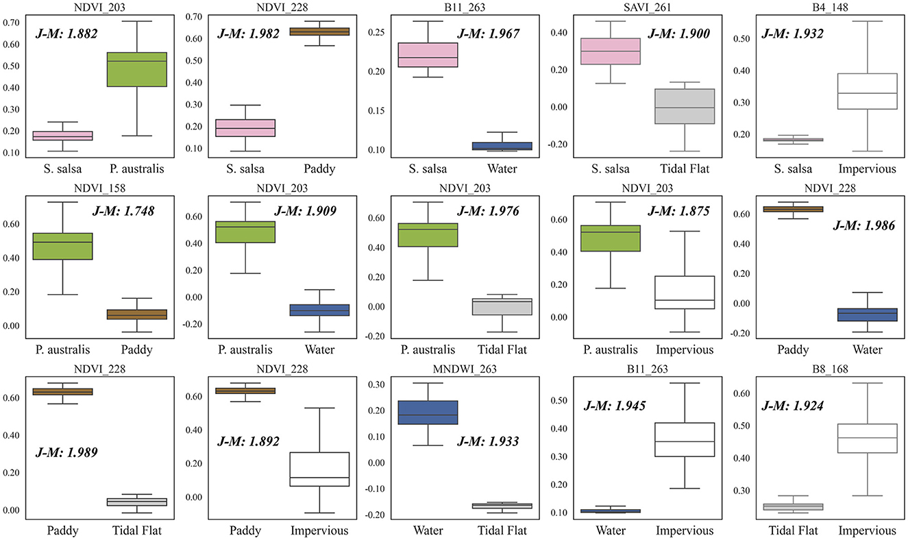
Figure 5. Separability and J-M distance of TOFs for different land cover pairs.
3.2 Random forest model
The RF model is an ensemble machine-learning algorithm known for its noise resistance, prevention of overfitting, and simplicity in model construction (Breiman, 2001). The algorithm provides a global explanation of each feature's contribution to accurate classification, allowing comparison of feature importance. The objectives of using the RF model in this study are: (1) to compare the importance of features across different feature sets, thereby confirming the effective capture of temporal remote sensing image information by TOFs; (2) to investigate differences in classification accuracy among three feature sets using typical machine learning algorithms, thus assessing the effectiveness of TOFs for classifying coastal wetlands; and (3) using the RF model with a small training sample, the study areas of 2017 and 2022 were pre-classified. A large-scale random sample set was generated for training and testing deep learning models via post-classification processing.
3.3 Residual neural network
CNN excels at remote sensing image classification, object recognition, and semantic segmentation due to its local feature extraction and spatial relationship modeling capabilities. While issues such as gradient vanishing and exploding limit its classification accuracy and training efficiency (Ma et al., 2019). ResNet addresses these issues by introducing residual connections (He et al., 2016), deepening networks, and improving model stability and training efficiency. The key of ResNet lies in its residual units and shortcut connections. Each residual unit comprises convolutional layers, batch normalization layers, and ReLU activation functions (Figure 6). The input x is processed through a shortcut, computes the residual feature F(x) = H(x) – x, and then adds it back to the input, resulting in the final output F(x) + x. This design ensures the network can learn new features while retaining original information.

Figure 6. Schematic diagram of the residual module.
This study adjusted the ResNet18 model to meet this study's specific feature input and output category requirements. Adjustments include adding a 3 × 3 convolutional layer at the input layer to handle multi-channel inputs equal to the number of features, retaining the residual blocks and pooling layers in the middle layers of ResNet18, and modifying the fully connected layer at the output layer to accommodate six output categories. The model training uses the Adam optimizer with a learning rate of 0.001 and the loss function as cross-entropy. After multiple training sessions and debugging, the study established 20 epochs as the training rounds for the model, with each batch size being 16. Under this configuration, the loss function stabilizes, indicating that the model's training process has converged. The model supports running on both GPU and CPU to ensure training efficiency and stability.
3.4 Accuracy assessment
Using a confusion matrix, this study evaluated the accuracy of coastal wetland mapping results in the LER. The accuracy metrics include user's accuracy (UA), which measures the proportion of correctly classified pixels for each class, and producer's accuracy (PA), which measures the proportion of correctly classified pixels for each class. Overall accuracy (OA) also represents the percentage of correctly classified pixels out of the total number of pixels. The confusion matrix is calculated by comparing each measured pixel in the reference image with the corresponding pixel in the classified image. The Kappa coefficient serves as a metric to evaluate the consistency of classification results, with values ranging from 0 to 1, where higher values indicate greater accuracy.
3.5 Ecological restoration effect evaluation
This study quantified the scale and sources of salt marsh vegetation ecological restoration using a land use transition matrix, distinguishing restoration into natural and artificial. Natural restoration was defined as converting natural land cover types to salt marsh vegetation, encompassing S. salsa, P. australis, tidal flat, inland water, and coastal water. Artificial restoration referred to converting artificial land use types to salt marsh vegetation, including paddies, reservoirs, aquaculture ponds, and impervious. This study evaluated the scale and direction of ecological restoration, clarified the relative contributions of natural regeneration and artificial restoration, and provided critical data support for formulating ecological restoration strategies.
4 Results
4.1 Analysis of TOFs
Figure 7 shows the ranking of the feature importance index, indicating that the accuracy of the RF model was enhanced by adding temporal information. Among the top 10 most important features, eight were temporal features, including five TOFs and three MCFs, along with two STFs, demonstrating the critical role of temporal information in model performance and the relative superiority of TOFs over MCFs and STFs. In the interval of the 10th to 20th most important features, STFs were predominant, with MCFs and TOFs each representing 2. Among the 10 least important features, MCFs constituted 6, while TOFs and STFs each comprised 2. Overall, the order of importance for the three types of features was TOFs > STFs > MCFs, and this ranking remained consistent across different model parameters (see S1 in Supplementary material).

Figure 7. Feature importance ranking results.
4.2 Classification accuracy analysis
The accuracy assessment results (Table 2) indicated that temporal features effectively enhance the overall classification accuracy of the RF model. Incorporating TOFs resulted in an 11.8% increase in OA of the RF model, accompanied by a Kappa coefficient improvement of 0.14. These enhancements surpassed the effects of MCFs on single-temporal-phase remote sensing image classification, which showed an 8.5% increase in OA and a 0.10 improvement in Kappa, respectively. The differences in accuracy highlighted the information disparities inherent in the two types of temporal features. Specifically, in terms of different land cover types (Figure 8), the inclusion of TOFs achieved the most improvement in PA for S. salsa (26.2%) and the most increase in UA for P. australis (28.3%). Meanwhile, there was no pronounced improvement in accuracy for water and tidal flat.
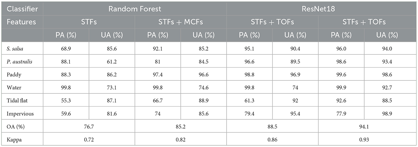
Table 2. Accuracy evaluation results.
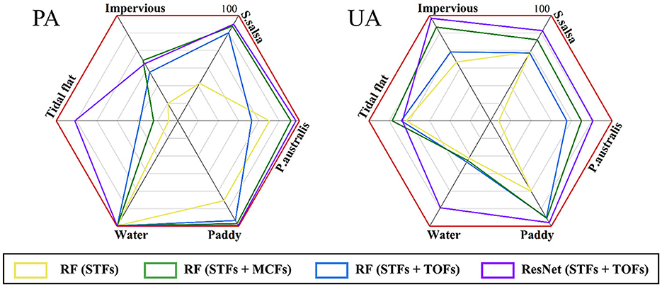
Figure 8. Accuracy improvement effect of temporal features and deep learning model on STFs. The (left panel) represents producer's accuracy, while the (right panel) represents user's accuracy.
From the perspective of classifiers, deep learning models demonstrated a clear accuracy advantage. Comparing the ResNet model to the RF model using the same input features, the ResNet model exhibited higher OA and Kappa coefficient values (Table 2). Additionally, the ResNet model improved accuracy across almost all land cover types (Figure 8). The RF model exhibited a lower PA for tidal flats, ranging from 55.3 to 61.3%. While the ResNet model improved this accuracy, achieving a PA of 92.6%. In terms of UA, the ResNet model enhanced the accuracy of water. Within the RF model, the classification accuracy for water ranged from 73.1 to 74.6%, indicating intense misclassification. In contrast, the ResNet model achieved a user's accuracy (UA) of 92.7% for water, suggesting better sensitivity to water pixels and a lower misclassification rate.
Figure 9 illustrates the classification results using TOFs and the ResNet model, while Figure 10 further displays four sites with complex land cover compositions to compare the effects of different classification strategies. Site 1 was characterized by numerous mixed pixels formed by abandoned roads and adjacent water channels. STFs identified these mixed pixels as paddy and S. salsa, leading to a “salt and pepper” noise in the classification results. Incorporating MCFs suppressed the noise, but some mixed pixels were still misclassified as paddy and S. salsa. Including TOFs improved this issue by correctly identifying some mixed pixels as built-up areas and roads, with fewer pixels misclassified as vegetation. The ResNet model achieved smoother classification results with more precise and more distinct contours of oil wells and surrounding transport roads. The disappearance of adjacent water channels and small abandoned roads may be attributed to the deep learning model's receptive field and parameter-sharing mechanisms. Specifically, omissions and oversights may occur when the network classifies tiny mixed pixels as the predominant surrounding categories due to parameter sharing.
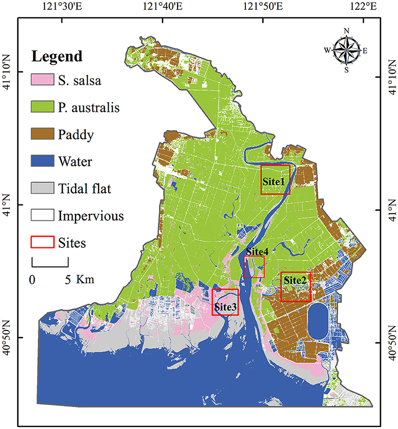
Figure 9. Classification results of coastal wetlands based on TOFs with the ResNet18 model. The red box indicates the zoom-in tiles comparison area.
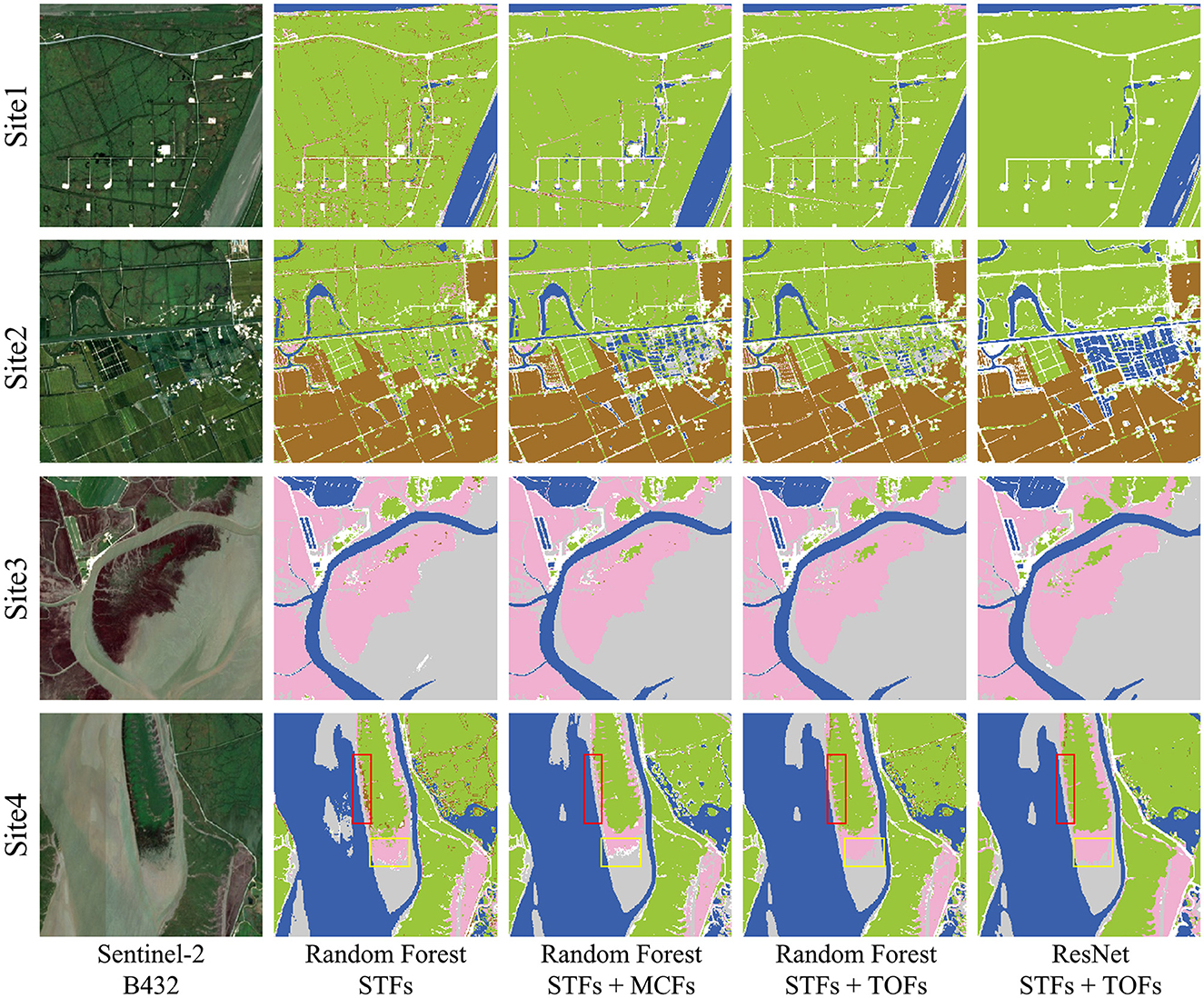
Figure 10. Detailed comparison of classification results from various methods.
The results for Site 2 show that STFs and the RF model may exhibit pixel confusion between P. australis and paddy. Adding temporal features (MCFs or TOFs) reduced this confusion but underestimated the extent of P. australis communities. In comparison, the ResNet model accurately identified the extent of P. australis communities. For Site 3, the RF model struggled with fragmented and small aquaculture ponds. In contrast, the ResNet model effectively extracted these ponds and their boundaries from the complex land cover.
The results for Site 4 show that rapid shifts in vegetation communities along environmental gradients between land and sea caused misclassifications. This transition from P. australis to S. salsa and then to tidal flat posed difficulties in accurately classifying coastal wetlands. Using STFs and the RF model, transition areas between P. australis and S. salsa were misclassified as paddies or impervious (as shown by the red box), and the transition areas between S. salsa and tidal flats were misclassified as impervious (as shown by the yellow box). Including MCFs reduced the misclassification between salt marsh vegetation and paddies, but confusion between S. salsa and tidal flats remained. The RF model with TOFs further reduced the confusion between salt marsh vegetation and tidal flats, but the misclassification between salt marsh vegetation and impervious still existed. Utilizing ResNet as the classifier effectively resolved the confusion in the transition areas between salt marsh vegetation types and between S. salsa and tidal flats while suppressing the “salt-and-pepper” effect, significantly improving the overall classification accuracy.
4.3 Temporal and spatial analysis of wetland type changes
According to Figure 11, from 2017 to 2022, the LER experienced substantial land cover changes, with the expansion of S. salsa and the retreat of aquaculture ponds being the most apparent changes. Table 3 shows that, from 2017 to 2022, aside from a notable increase in salt marsh vegetation, other land cover types either decreased or remained stable during this period. The area of salt marsh vegetation in the LER increased from 42,330.68 hectares to 53,655.2 hectares, representing a rise of 26.75%. Specifically, S. salsa expanded from 2,682.96 hectares to 5,142.71 hectares, with a growth of 91.68% (2,459.75 hectares). P. australis also grew significantly, increasing by 8,862.77 hectares, or 22.35%. Conversely, the area of aquaculture ponds contracted from 7,808.03 hectares to 4,073.83 hectares, with a reduction of 47.83%. Inland water and tidal flats decreased by 30.80 and 22.89%, respectively. The area of paddy fields decreased from 13,670.31 hectares to 10,967.85 hectares, representing a 19.77% reduction. Impervious decreased from 11,940.21 hectares to 10,815.37 hectares, a decrease of 9.42%. Coastal water and reservoirs showed minimal change, fluctuating within ±1%. Overall, these data indicated a substantial expansion of salt marsh vegetation and decreased human activity, highlighting the impact of ecological protection and restoration efforts.

Figure 11. Comparative land cover change in the LER. (A) Year 2017, (B) Year 2022.
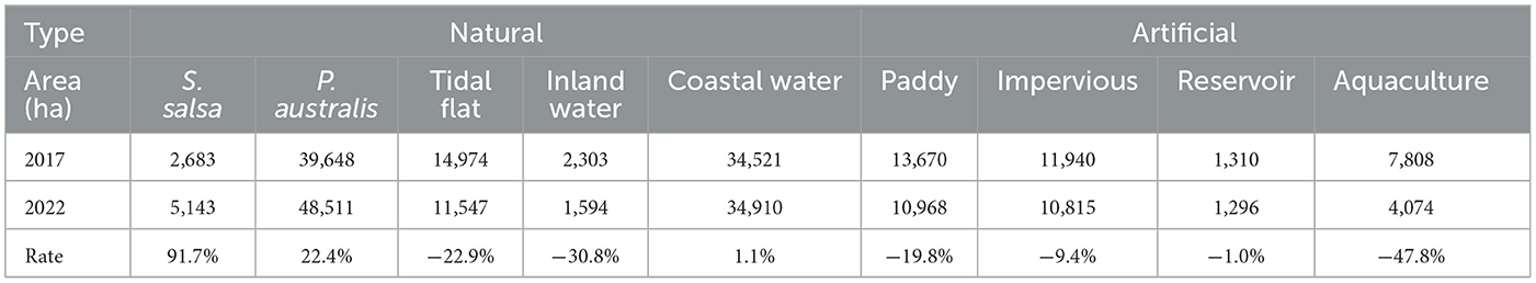
Table 3. Dynamic changes in land cover in the LER from 2017 to 2022.
Table 4 shows that artificial restoration was the primary driver of the growth in salt marsh vegetation areas in the LER. Among the newly added salt marsh vegetation, 65.91% originated from the conversion of artificial land use types, while 34.09% came from the conversion of natural land cover types. In terms of spatial distribution (Figure 12), naturally restored S. salsa is more dispersed, mainly distributed on both sides of the Liaohe Estuary and at the boundary between P. australis and tidal flats. In contrast, artificially restored S. salsa is predominantly concentrated west of the Liaohe Estuary, where aquaculture facilities were removed. This suggests that ecological protection projects have had a crucial impact on salt marsh vegetation restoration.
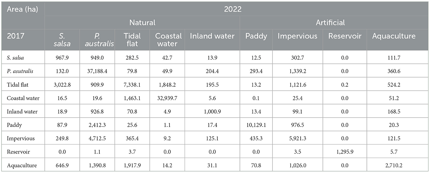
Table 4. Land cover transition matrix of the study area from 2017 to 2022.
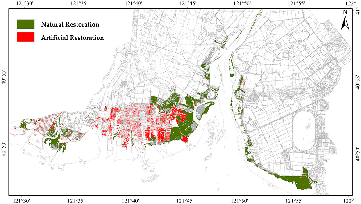
Figure 12. Spatial distribution of S. salsa restoration. Red indicates restored S. salsa converted from human land use, i.e., artificial Restoration; green represents restored S. salsa converted from natural wetlands, i.e., natural restoration.
The reduction in aquaculture area was another obvious change. According to Table 4, from 2017 to 2022, more than half of the original aquaculture areas were converted into natural wetlands. Among them, tidal flats, P. australis, and S. salsa accounted for 24.56, 17.81, and 8.29% of the converted aquaculture area, respectively. Additionally, there was a reduction in paddy and impervious areas, with P. australis and S. salsa being the common primary outflow directions, indicating the restoration of wetland ecosystems. These changes reflect significant achievements in ecological conservation efforts in the LER over the past few years.
5 Discussion
5.1 Time-series remote sensing image analysis method
Previous studies have demonstrated that utilizing time-series remote sensing imagery can improve the accuracy of wetland mapping. However, the selection of image acquisition times still requires further discussion. Henderson and Lewis (2008) emphasized that increasing the number of images can improve classification accuracy to a certain extent, whereas selecting KTPs is more crucial. Existing temporal feature extraction methods neglect this issue, which may lead to the loss of critical information or the introduction of misleading information, thus affecting classification accuracy. Compared to previous research, this study proposed a temporal feature extraction method based on S-G filtering. By analyzing the variations in temporal curves of different land cover types, this method identified KTPs. Subsequently, TOFs were extracted from these KTPs using the J-M distance to enhance the discriminability among different wetland types.
The results demonstrated that TOFs had evident advantages over STFs and MCFs in terms of feature importance and classification accuracy. This suggests that TOFs contain more crucial information and are more effective for accurately classifying the model. Specifically, including TOFs resulted in an 11.8% increase in the classification accuracy of the RF model and a 0.14 increase in the Kappa coefficient. In contrast, the improvements for MCFs were only 8.5% and 0.10, respectively. Moreover, using TOFs significantly improved the accuracy of specific land covers: the PA of S. salsa increased by 26.2%, and the UA of P. australis increased by 28.3%. The advantage of TOFs was evident in resolving the confusion in the transition areas between salt marsh vegetation and salt marsh vegetation to tidal flats, leading to more accurate classification results.
5.2 Deep learning model and time-series remote sensing images
Conventional ResNet models were primarily applied to spectral or spatial domains, with limited consideration given to the time dimension, which restricted their ability to leverage the temporal information of remote sensing images. This study integrated TOFs with ResNet, providing crucial temporal information. ResNet, extending the CNN framework, introduced residual connections to extract spatial structural features through convolutional kernels. Additionally, it employed pooling layers to reduce noise and mitigate the “salt-and-pepper” effect, enhancing the model's adaptability to the complexity of coastal wetland ecosystems. This approach profoundly improved classification accuracy by leveraging the spatial and temporal information of remote sensing images. The research findings can serve as a robust reference for future studies exploring deep learning methods based on temporal features. Through the combination of TOFs and deep learning models, this study acquired high-resolution spatial distribution information and fine wetland mapping in the LER.
A dependency accompanies deep learning models' accuracy advantage on massive annotated sample datasets and storage and computing resources, which limits their application in remote sensing. In this study, we utilized the GEE platform to accomplish sample augmentation and convolutional sampling (Figure 13), efficiently obtaining large-scale sample datasets for training and validating deep learning models. Despite rigorous manual inspection and modification, sample augmentation strategies may still introduce potential biases in validation samples. Therefore, future research could explore methods such as sample transfer, weakly supervised learning, or unsupervised learning to reduce the dependence of deep learning on large annotated datasets.
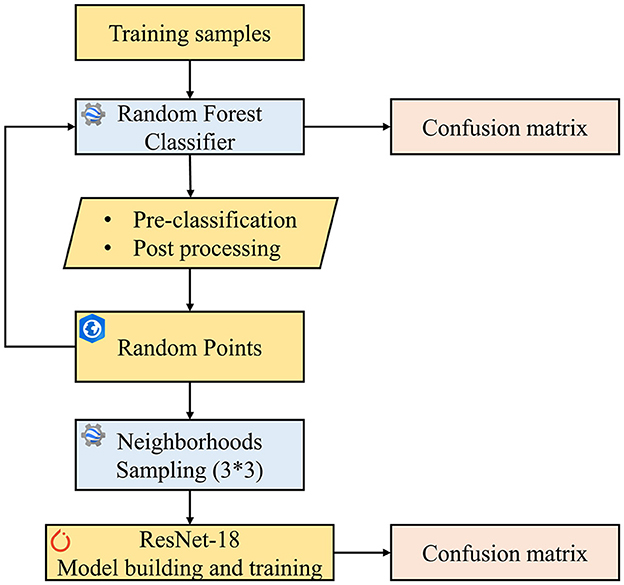
Figure 13. Utilizing GEE to provide data foundation for deep learning model training.
5.3 Ecological restoration effect evaluation
This study showed apparent changes in land cover types in the LER from 2017 to 2022 by comparing land cover mapping results. Specifically, it demonstrated the extensive recovery of salt marsh vegetation and the substantial reduction in aquaculture areas, consistent with the findings of Zhang G. et al. (2023), indicating effective improvement in the wetland ecosystem of the study area. Furthermore, using a land use transfer matrix, this study identified the dominant role of artificial restoration in the ecological restoration process of salt marsh vegetation in the LER, providing strong evidence for the significant achievements in ecological conservation efforts in the region in recent years. The research results indicated that since the implementation of prohibition management in the LER in 2017, the impact of human activities has gradually decreased, and the area of anthropogenic land cover types has significantly reduced.
This study revealed the sources of S. salsa ecological restoration by using a land use transfer matrix based on different original land cover types (such as artificial surfaces like impervious, paddy, aquaculture, reservoirs, and natural surfaces like inland water, coastal water, tidal flat, and P. australis). This method simplified differentiating between natural and artificial restoration; however, the intricate interplay between the two posed challenges for a clear distinction. In practical ecological restoration projects, artificial and natural restoration often occur interchangeably. In the initial stages of a project, artificial restoration may be employed to accelerate the restoration process. In later stages, as the ecosystem stabilizes, there is greater reliance on natural restoration. This combined strategy complicates the distinction between artificial and natural restoration efforts. Moreover, complex interactions exist between artificial and natural restoration. For instance, environmental restoration projects may provide conditions conducive to natural restoration, while natural restoration could also be an indirect consequence of human intervention (Li et al., 2023). Therefore, future research should further explore the factors and mechanisms influencing wetland ecosystem restoration and develop more scientifically rigorous methods to ensure the success of ecological system restoration projects.
5.4 Influence of tidal variations on tidal flat range and boundaries in coastal wetlands
The method employed in this study still has limitations in addressing the influence of tidal variations on the range and boundaries of tidal flats. Future improvements could include integrating multi-source image fusion, enhancing the density of temporal image stacks, and combining tidal schedules to select remote sensing images during low tide states, thus mitigating the effects of tidal changes. In addition, exploring more advanced temporal analysis methods is essential. For instance, Zhi et al. (2022) developed a tidal flat wetland classification algorithm based on temporal remote sensing indices using the GEE platform, accurately extracting the extent of tidal flats using water frequency indices. He et al. (2023) proposed a tidal flat identification index based on spectral reflectance differences between tidal flats and other land cover types, achieving good extraction accuracy in tidal flat mapping. Jia et al. (2021) developed a method combining maximum spectral indices composite with the Otsu algorithm to produce a tidal flat map of China at a 10-meter resolution (China_Tidal Flat, CTF). These studies serve as crucial references for refining tidal flat classification and identification methodologies, providing valuable insights for further optimizing this study.
6 Conclusion
Aiming at the challenges posed by the dynamism and complexity of coastal wetlands for precise mapping, this study developed a novel mapping method using time-series remote sensing images and a deep learning model. This method achieved precise mapping and change analysis of the LER, revealing the ecological restoration effects and primary sources within the study area from 2017 to 2022. The results demonstrate that TOFs, constructed with S-G filtering and J-M distance, outperform commonly used MCFs in feature importance and classification accuracy. This highlights the superior capability of TOFs to capture essential information in time-series remote sensing images, enhancing precise mapping of coastal wetlands. The results indicate that by incorporating TOFs into the ResNet model, temporal and spatial information were effectively integrated, improving coastal wetlands' mapping accuracy and classification precision. Moreover, by comparing land cover mapping results from 2017 to 2022 in the Liaohe Estuary wetlands, this study identified trends in ecological restoration and highlighted the dominant role of artificial restoration in rehabilitating salt marsh vegetation in the region.
This study highlights the importance of selecting KTPs and optimized features to improve classification accuracy. The effectiveness of integrating time-series remote sensing image analysis with a deep learning model in complex coastal wetland mapping was also validated. Furthermore, the findings of this study provide valuable technical support for the accurate monitoring of coastal wetland ecosystems and offer essential data for ecological protection and restoration efforts. These contributions are crucial for promoting sustainable development in coastal zones amidst the challenges posed by global climate change. Future research can mitigate the effects of tidal variations by fusing multi-source remote sensing images or temporal remote sensing indices to obtain more accurate tidal flat boundaries. Advanced algorithms like transfer learning can further enhance the efficiency and accuracy of deep learning models by reducing sample bias during training. Moreover, future studies should further analysis the factors and mechanisms influencing wetland ecosystem restoration, accurately distinguishing between artificial and natural restoration effects to better understand their impacts. This comprehensive understanding will guide ecological conservation and restoration efforts, improve their efficiency and sustainability, and facilitate the healthy development of coastal ecosystems.
Data availability statement
The original contributions presented in the study are included in the article/Supplementary material, further inquiries can be directed to the corresponding author.
Author contributions
LK: Conceptualization, Data curation, Formal analysis, Funding acquisition, Investigation, Methodology, Writing – review & editing. YL: Data curation, Formal analysis, Investigation, Methodology, Resources, Software, Visualization, Writing – original draft, Writing – review & editing. QT: Resources, Software, Supervision, Validation, Writing – review & editing. YZ: Writing – review & editing. QW: Formal analysis, Funding acquisition, Writing – review & editing.
Funding
The author(s) declare financial support was received for the research, authorship, and/or publication of this article. This research was funded by the National Natural Science Foundation of China (Nos. 42076222, 42276231, 42201070), Sub-project of National Key Research and Development Program of China (No. 2022YFC3106101), Natural Science Foundation of Liaoning Province, China (No. 2021-MS-274), and Social Science Federation Project of Liaoning Province (No. 2024lslybkt-038).
Conflict of interest
The authors declare that the research was conducted in the absence of any commercial or financial relationships that could be construed as a potential conflict of interest.
Publisher's note
All claims expressed in this article are solely those of the authors and do not necessarily represent those of their affiliated organizations, or those of the publisher, the editors and the reviewers. Any product that may be evaluated in this article, or claim that may be made by its manufacturer, is not guaranteed or endorsed by the publisher.
Supplementary material
The Supplementary Material for this article can be found online at: https://www.frontiersin.org/articles/10.3389/ffgc.2024.1409985/full#supplementary-material
References
Cai, Z., Jönsson, P., Jin, H., and Eklundh, L. (2017). Performance of smoothing methods for reconstructing NDVI time-series and estimating vegetation phenology from MODIS data. Remote Sens. 9:1271. doi: 10.3390/rs9121271
Cheng, X., Sun, Y., Zhang, W., Wang, Y., Cao, X., and Wang, Y. (2023). Application of deep learning in multitemporal remote sensing image classification. Remote Sens. 15:3859. doi: 10.3390/rs15153859
Gong, P., Niu, Z., Cheng, X., Guo, J., Liang, L., Wang, X., et al. (2010). China's wetland change (1990–2000) determined by remote sensing. Sci. China Earth Sci. 53, 1036–1042. doi: 10.1007/s11430-010-4002-3
Gong, P., Zhang, W., Yu, L., Li, C., Wang, J., Liang, L., et al. (2016). New research paradigm for global land cover mapping. Natl. Remote Sens. Bull. 20, 1002–1016. doi: 10.11834/jrs.20166138
Günen, M. A. (2022). Performance comparison of deep learning and machine learning methods in determining wetland water areas using EuroSAT dataset. Environ. Sci. Pollut. Res. 29, 21092–21106. doi: 10.1007/s11356-021-17177-z
He, K., Zhang, X., Ren, S., and Sun, J. (2016). “Deep residual learning for image recognition,” in Proceedings of the IEEE Conference on Computer Vision and Pattern Recognition, 770–778. Available online at: http://openaccess.thecvf.com/content_cvpr_2016/html/He_Deep_Residual_Learning_CVPR_2016_paper.html (accessed December 15, 2023).
He, T., Xia, Q., Zhang, H., Zheng, Q., Zhu, H., Deng, X., et al. (2023). Development of a tidal flat recognition index based on multispectral images for mapping tidal flats. Ecol. Indic. 157:111218. doi: 10.1016/j.ecolind.2023.111218
Henderson, F. M., and Lewis, A. J. (2008). Radar detection of wetland ecosystems: a review. Int. J. Remote Sens. 29, 5809–5835. doi: 10.1080/01431160801958405
Heydari, S. S., and Mountrakis, G. (2018). Effect of classifier selection, reference sample size, reference class distribution and scene heterogeneity in per-pixel classification accuracy using 26 Landsat sites. Remote Sens. Environ. 204, 648–658. doi: 10.1016/j.rse.2017.09.035
Jamali, A., Mahdianpari, M., Brisco, B., Granger, J., Mohammadimanesh, F., and Salehi, B. (2021a). Wetland mapping using multi-spectral satellite imagery and deep convolutional neural networks: a case study in Newfoundland and Labrador, Canada. Can. J. Remote Sens. 47, 243–260. doi: 10.1080/07038992.2021.1901562
Jamali, A., Mahdianpari, M., Mohammadimanesh, F., Brisco, B., and Salehi, B. (2021b). A synergic use of Sentinel-1 and Sentinel-2 Imagery for complex wetland classification using Generative Adversarial Network (GAN) scheme. Water 13:3601. doi: 10.3390/w13243601
Jia, M., Wang, Z., Mao, D., Ren, C., Wang, C., and Wang, Y. (2021). Rapid, robust, and automated mapping of tidal flats in China using time series Sentinel-2 images and Google Earth Engine. Remote Sens. Environ. 255:112285. doi: 10.1016/j.rse.2021.112285
Kovács, G. M., Horion, S., and Fensholt, R. (2022). Characterizing ecosystem change in wetlands using dense earth observation time series. Remote Sens. Environ. 281:113267. doi: 10.1016/j.rse.2022.113267
Li, H., Mao, D., Wang, Z., Huang, X., Li, L., and Jia, M. (2022). Invasion of Spartina alterniflora in the coastal zone of mainland China: control achievements from 2015 to 2020 towards the Sustainable Development Goals. J. Environ. Manage. 323:116242. doi: 10.1016/j.jenvman.2022.116242
Li, H., Wang, C., Cui, Y., and Hodgson, M. (2021). Mapping salt marsh along coastal South Carolina using U-Net. ISPRS J. Photogramm. Remote Sens. 179, 121–132. doi: 10.1016/j.isprsjprs.2021.07.011
Li, L., Huang, X., and Yang, H. (2023). A new framework for identifying ecological conservation and restoration areas to enhance carbon storage. Ecol. Indic. 154:110523. doi: 10.1016/j.ecolind.2023.110523
Liu, R., and Li, J. (2021). Classification of Yancheng coastal wetland vegetation based on vegetation phenological characteristics derived from Sentinel-2 time-series. Acta Geogr. Sin. 76, 1680–1692. doi: 10.11821/dlxb202107008
Liu, R., Liang, S., Zhao, H., Qi, G., Li, L., Jiang, Y., et al. (2017). Progress of China coastal wetland based on remote sensing. Remote Sens. Technol. Appl. 32, 998–1011. doi: 10.11873/j.issn.1004-0323.2017.6.0998
Ludwig, C., Walli, A., Schleicher, C., Weichselbaum, J., and Riffler, M. (2019). A highly automated algorithm for wetland detection using multi-temporal optical satellite data. Remote Sens. Environ. 224, 333–351. doi: 10.1016/j.rse.2019.01.017
Ma, L., Liu, Y., Zhang, X., Ye, Y., Yin, G., and Johnson, B. A. (2019). Deep learning in remote sensing applications: a meta-analysis and review. ISPRS J. Photogramm. Remote Sens. 152, 166–177. doi: 10.1016/j.isprsjprs.2019.04.015
Ma, Z., Melville, D. S., Liu, J., Chen, Y., Yang, H., Ren, W., et al. (2014). Rethinking China's new great wall. Science 346, 912–914. doi: 10.1126/science.1257258
Mahdianpari, M., Granger, J. E., Mohammadimanesh, F., Salehi, B., Brisco, B., Homayouni, S., et al. (2020). Meta-analysis of wetland classification using remote sensing: a systematic review of a 40-year trend in North America. Remote Sens. 12:1882. doi: 10.3390/rs12111882
Mao, D., Luo, L., Wang, Z., Wilson, M. C., Zeng, Y., Wu, B., et al. (2018a). Conversions between natural wetlands and farmland in China: a multiscale geospatial analysis. Sci. Total Environ. 634, 550–560. doi: 10.1016/j.scitotenv.2018.04.009
Mao, D., Wang, Z., Jia, M., Luo, L., Niu, Z., Jiang, W., et al. (2023). Review of global studies on the remote sensing of wetlands from 1975 to 2020. Natl. Remote Sens. Bull. 27, 1270–1280. doi: 10.11834/jrs.20231022
Mao, D., Wang, Z., Wu, J., Wu, B., Zeng, Y., Song, K., et al. (2018b). China's wetlands loss to urban expansion. Land Degrad. Dev. 29, 2644–2657. doi: 10.1002/ldr.2939
Murray, N. J., Phinn, S. R., DeWitt, M., Ferrari, R., Johnston, R., Lyons, M. B., et al. (2019). The global distribution and trajectory of tidal flats. Nature 565, 222–225. doi: 10.1038/s41586-018-0805-8
National Research Council Division on Earth and Life Studies, Commission on Geosciences, Environment and Resources, Committee on Characterization of Wetlands. (1995). Wetlands: Characteristics and Boundaries. National Academies Press.
Ni, R., Tian, J., Li, X., Yin, D., Li, J., Gong, H., et al. (2021). An enhanced pixel-based phenological feature for accurate paddy rice mapping with Sentinel-2 imagery in Google Earth Engine. ISPRS J. Photogramm. Remote Sens. 178, 282–296. doi: 10.1016/j.isprsjprs.2021.06.018
Niu, Z., Zhang, H., Wang, X., Yao, W., Zhou, D., Zhao, K., et al. (2012). Mapping wetland changes in China between 1978 and 2008. Chin. Sci. Bull. 57, 2813–2823. doi: 10.1007/s11434-012-5093-3
O'Neil, G. L., Goodall, J. L., Behl, M., and Saby, L. (2020). Deep learning using physically-informed input data for wetland identification. Environ. Model. Softw. 126:104665. doi: 10.1016/j.envsoft.2020.104665
Ren, C., Wang, Z., Zhang, Y., Zhang, B., Chen, L., Xi, Y., et al. (2019). Rapid expansion of coastal aquaculture ponds in China from Landsat observations during 1984–2016. Int. J. Appl. Earth Obs. Geoinf. 82:101902. doi: 10.1016/j.jag.2019.101902
Schafer, R. W. (2011). What Is a Savitzky-Golay filter? IEEE Signal Process. Mag. 28, 111–117. doi: 10.1109/MSP.2011.941097
Sun, C., Li, J., Liu, Y., Liu, Y., and Liu, R. (2021). Plant species classification in salt marshes using phenological parameters derived from Sentinel-2 pixel-differential time-series. Remote Sens. Environ. 256:112320. doi: 10.1016/j.rse.2021.112320
Tan, Y., Yang, Q., Jia, M., Xi, Z., Wang, Z., and Mao, D. (2022). Remote sensing monitoring and analysis of the impact of human activities on wetland in Liaohe Estuary National Nature Reserve. Remote Sens. Technol. Appl. 37, 218–230. doi: 10.3390/rs14205273
Verbesselt, J., Hyndman, R., Newnham, G., and Culvenor, D. (2010). Detecting trend and seasonal changes in satellite image time series. Remote Sens. Environ. 114, 106–115. doi: 10.1016/j.rse.2009.08.014
Wang, M., Mao, D., Wang, Y., Li, H., Zhen, J., Xiang, H., et al. (2024). Interannual changes of urban wetlands in China's major cities from 1985 to 2022. ISPRS J. Photogramm. Remote Sens. 209, 383–397. doi: 10.1016/j.isprsjprs.2024.02.011
Wang, M., Mao, D., Wang, Y., Xiao, X., Xiang, H., Feng, K., et al. (2023). Wetland mapping in East Asia by two-stage object-based Random Forest and hierarchical decision tree algorithms on Sentinel-1/2 images. Remote Sens. Environ. 297:113793. doi: 10.1016/j.rse.2023.113793
Wang, Y., Hollingsworth, P. M., Zhai, D., West, C. D., Green, J. M. H., Chen, H., et al. (2023). High-resolution maps show that rubber causes substantial deforestation. Nature 623, 340–346. doi: 10.1038/s41586-023-06642-z
Wang, Z., Wu, J., Madden, M., and Mao, D. (2012). China's wetlands: conservation plans and policy impacts. Hyperspectral Image Data 41, 782–786. doi: 10.1007/s13280-012-0280-7
Wen, Q., Zhang, Z., Xu, J., Zuo, L., Wang, X., Liu, B., et al. (2011). Spatial and temporal change of wetlands in Bohai rim during 2000-2008: an analysis based on satellite images. Natl. Remote Sens. Bull. 15, 183–200. doi: 10.11834/jrs.20110115
Wu, L., and Wu, W. (2023). The optimum time window for spartina alterniflora classification based on the filtering algorithm and vegetation phenology using GEE. Geo Inf. Sci. 25, 606–624. doi: 10.12082/dqxxkx.2023.220672
Xiang, M., Wei, W., and Wu, W. (2018). Review of vegetation phenology estimation by using remote sensing. China Agric. Inf. 30, 55–66. doi: 10.12105/j.issn.1672-0423.20180106
Xie, Z., and Zhang, C. (2023). Reviews of methods for vegetation phenology monitoring from remote sensing data. Remote Sens. Technol. Appl. 38, 1–14. doi: 10.11873/j.issn.1004-0323.2023.1.0001
Xu, W., Fan, X., Ma, J., Pimm, S. L., Kong, L., Zeng, Y., et al. (2019). Hidden loss of wetlands in China. Curr. Biol. 29, 3065–3071. doi: 10.1016/j.cub.2019.07.053
Zhang, G., Cai, Y., Yang, Y., Yan, J., Sun, J., Wang, Q., et al. (2023). Evaluation of landscape stability and vegetation carbon storage value in Liaohe delta coastal wetland. Mar. Environ. Sci. 42, 612–621. doi: 10.12111/j.mes.2022-x-0312
Zhang, W., Tang, P., and Zhang, Z. (2023). Time series classification of remote sensing data based on temporal self-attention mechanism. Natl. Remote Sens. Bull. 27, 1914–1924. doi: 10.11834/jrs.20210453
Zhang, X., Liu, L., Zhao, T., Chen, X., Lin, S., Wang, J., et al. (2022). GWL_FCS30: global 30 m wetland map with fine classification system using multi-sourced and time-series remote sensing imagery in 2020. Earth Syst. Sci. Data Discuss. 2022, 1–31. doi: 10.5194/essd-2022-180
Zhang, X., Liu, L., Zhao, T., Wang, J., Liu, W., and Chen, X. (2024). Global annual wetland dataset at 30 m with a fine classification system from 2000 to 2022. Sci. Data 11:310. doi: 10.1038/s41597-024-03143-0
Zhi, C., Wu, W., and Su, H. (2022). Mapping the intertidal wetlands of Fujian Province based on tidal dynamics and vegetational phonology. Natl. Remote Sens. Bull. 26, 373–385. doi: 10.11834/jrs.20210586
Keywords: coastal vegetation, classification, phenological characterization of vegetation communities, time-series analysis, remote sensing, deep learning, ecological restoration
Citation: Ke L, Lu Y, Tan Q, Zhao Y and Wang Q (2024) Precise mapping of coastal wetlands using time-series remote sensing images and deep learning model. Front. For. Glob. Change 7:1409985. doi: 10.3389/ffgc.2024.1409985
Received: 31 March 2024; Accepted: 27 May 2024;
Published: 10 June 2024.
Edited by:
Wenting Wu, Fuzhou University, ChinaCopyright © 2024 Ke, Lu, Tan, Zhao and Wang. This is an open-access article distributed under the terms of the Creative Commons Attribution License (CC BY). The use, distribution or reproduction in other forums is permitted, provided the original author(s) and the copyright owner(s) are credited and that the original publication in this journal is cited, in accordance with accepted academic practice. No use, distribution or reproduction is permitted which does not comply with these terms.
*Correspondence: Quanming Wang, cW13YW5nQG5tZW1jLm9yZy5jbg==