 LeeAnn Haaf
 Salli F. Dymond
- 1Partnership for the Delaware Estuary Inc., Wilmington, DE, United States
- 2Department of Biodiversity, Earth and Environmental Science, Drexel University, Philadelphia, PA, United States
- 3School of Forestry, Northern Arizona University, Flagstaff, AZ, United States
Introduction: Coastal forests occupy low-lying elevations, typically adjacent to tidal salt marshes. Exposed to increased flooding with sea level rise, coastal forests have retreated as salt marshes advance upslope. Coastal forests likely currently experience periodic tidal flooding, but whether they temporarily accommodate or quickly succumb to rising sea level under changing climatic conditions remains a complex question. Disentangling how tidal flooding and climate affect tree growth is important for gauging which coastal forests are most at risk of loss with increasing sea levels.
Methods: Here, dendrochronology was used to study tree growth relative to climate variables and tidal flooding. Specifically, gradients in environmental conditions were compared to species-specific (Pinus taeda, Pinus rigida, Ilex opaca) growth in coastal forests of two estuaries (Delaware and Barnegat Bays). Gradient boosted linear regression, a machine learning approach, was used to investigate tree growth responses across gradients in temperature, precipitation, and tidal water levels. Whether tree ring widths increased or decreased with changes in each parameter was compared to predictions for seasonal climate and mean high water level to identify potential vulnerabilities.
Results: These comparisons suggested that climate change as well as increased flood frequency will have mixed, and often non-linear, effects on coastal forests. Variation in responses was observed across sites and within species, supporting that site-specific conditions have a strong influence on coastal forest response to environmental change.
Discussion: Site- and species-specific factors will be important considerations for managing coastal forests given increasing tidal flood frequencies and climatic changes.
1 Introduction
Coastal forests, or those occupying supratidal lands adjacent to tidal marshes, experience periodic flooding that influence their health and longevity. Forests retreat upslope as trees die with increased flooding by sea level rise (SLR) adjacent to tidal marsh borders, eventually allowing tidal marshes to migrate inland. Dead trees are already a prominent part of many marsh-forest ecotones (Smith, 2013; White et al., 2021). Although the outcome is clear (i.e., tree death), the ecological thresholds, time frames, and development of forest retreat is less so. Land slope is likely a key driver of retreat rates, but some studies show variability in low slope areas (see Smith, 2013; Schieder et al., 2018; Sacatelli et al., 2023). Mature trees can also possibly survive decades between when saltwater flooding begins and mortality occurs (Kirwan et al., 2007; Hall et al., 2022; Chen and Kirwan, 2023). In New Jersey, USA, sea levels are likely to rise 60 cm over the next 80 years (Kopp et al., 2019) and, as a result, trees in coastal forests are increasingly at risk of mortality due to saltwater exposure (Zhang et al., 2021; McDowell et al., 2022). How trees respond to environmental conditions will be important for predicting where or when existing coastal forests die back with SLR. For coastal managers, understanding when a forest might succumb to increasing floods will be important to plan for landscape changes in the next century as climates change and SLR accelerates.
Changing climatic conditions, in addition to increasing flood frequencies, add additional complexity to whether coastal forests might temporarily accommodate or quickly succumb to rising sea levels. In the broader US Northeast region, which includes the Mid Atlantic, air and oceanic temperatures are likely to increase and precipitation events may become more intense (Dupigny-Giroux et al., 2018). These changes will have direct consequences to tree phenology and resilience across the Mid Atlantic (Butler-Leopold et al., 2018), but species-specific vulnerability will likely drive variations in responses to changing conditions (Swanston et al., 2018). For tree species situated at their southernmost ranges, for example, warming temperatures could increase the probability of mature trees suffering from concurrent heat and flooding, since unrelated yet simultaneous disturbance events can exacerbate stress (Niinemets, 2010). Tree species already at their northern range limits, however, might gain resilience as temperatures rise. For these trees, warming might reduce the probability of temperature-related stress occurring contemporaneously with coastal floods. It stands to reason that climatic effects on tree growth would influence predictions of coastal forest retreat to SLR, yet recent mapping efforts find that these influences can be complex or not significant across a marsh-forest ecotone (Chen and Kirwan, 2022, Molino et al., 2023).
How environmental conditions affect tree growth is important for gauging which coastal forests are most at risk of retreat with climate change and increasing sea levels. Deviations from species-specific environmental optima reduce tree growth, with repeated growth reductions signaling increasing tree stress (Ogle et al., 2000; Bigler and Bugmann, 2004; Niinemets, 2010). If stressful conditions persist, mortality results (Bigler and Bugmann, 2004). Thus, the relative risk of mortality due to SLR in extant coastal forests can be studied by measuring tree growth over time. Dendrochronology is a useful tool to study growth relative to climate and tidal flooding in the Mid Atlantic. While improved mapping may help further refine spatial patterns in forest stress and retreat (Chen and Kirwan, 2022, 2023), dendrochronology offers an additional perspective for analyzing how the intricacies of past environmental conditions affected tree growth. Predictions on future growth might also be developed by comparing growth-condition relationships over past decades (Lloyd et al., 2013; Gu et al., 2019). Dendrochronological studies can supplement mapping or ecological studies by providing an understanding of which factors induce tree stress in low-lying coastal forests, which in turn helps predict critical points in tree stress or mortality and, therefore, forest retreat.
Dendrochronology was used here to study how gradients in environmental conditions affect species-specific (Pinus taeda, Pinus rigida, Ilex opaca) growth in coastal forests of two estuaries (Delaware and Barnegat Bays). Haaf et al. (2021) previously reported on correlations with climatic conditions and tidal water levels at these same sites, but correlation results can be limited in scope. For instance, correlation tests fail to detect non-linear relationships that are common in tree responses to environmental conditions (Anderson-Teixeira et al., 2022). Correlation tests are nonetheless important for a general understanding of tree responses, like those needed for climatic reconstructions, but on an ecological level, additional syntheses could elucidate variability in forest vulnerability to retreat under rising sea level. This study examines how coastal flooding and climatic factors influence tree growth in coastal forests using gradient boosted regressions, in addition to some linear analyses. Gradient boosting improves regression models through an iterative, algorithmic machine learning process (Elith et al., 2008). Gradient boosted regressions offer more power than simple linear-based tests (e.g., Pearson correlations) to find relationships among multiple parameters with complications such as collinearity, non-linearity, and autoregression (Elith et al., 2008; Dormann et al., 2013; Lloyd et al., 2013; Gu et al., 2019). We chose gradient boosted regressions given their use and higher performance compared to other models in previous tree ring research (Lloyd et al., 2013; Fang et al., 2015; Gu et al., 2019; Sahour et al., 2021; Kuhl et al., 2023). From gradient boosted results, we also develop baselines from which to anticipate how changing conditions, in both climate and coastal flooding, might affect the future growth of trees in coastal forests.
2 Materials and methods
2.1 Study sites and study species
We based our analyses on trees sampled from four coastal forest study sites — two each in the Delaware Bay and Barnegat Bay in the US Mid Atlantic (Figure 1). Sites were selected by gentleness of slope, proximity to intertidal marshes, possible inundation if sea levels rose 1.2 m (which is approximately the most recent maximum tide level in Lewes, DE as a result of Hurricane Sandy in 2012; Fanelli et al., 2013), and the abundance of large diameter, low elevation trees (Figure 2 and Haaf et al., 2021). We used previously published dendrochronological records from loblolly pine (Pinus taeda L.), pitch pine (Pinus rigida Mill.), and American holly (Ilex opaca Aiton) for this study (Haaf et al., 2021; Table 1, Figure 2, and Supplementary Figure 1). In Delaware Bay, 51 loblolly pines were cored at Jakes Landing, NJ (39.178°N, −74.853°W) and 60 American hollies were cored at the St Jones Delaware National Estuarine Research Reserve, DE (39.089°N, −75.439°W). In Barnegat Bay, 51 pitch pines were cored at Cattus Island, NJ (39.981°N, −74.128°W) and 51 American hollies were cored at the Lighthouse Center, NJ (39.089°N, −75.439°W). Additional descriptions are in Haaf et al. (2021).
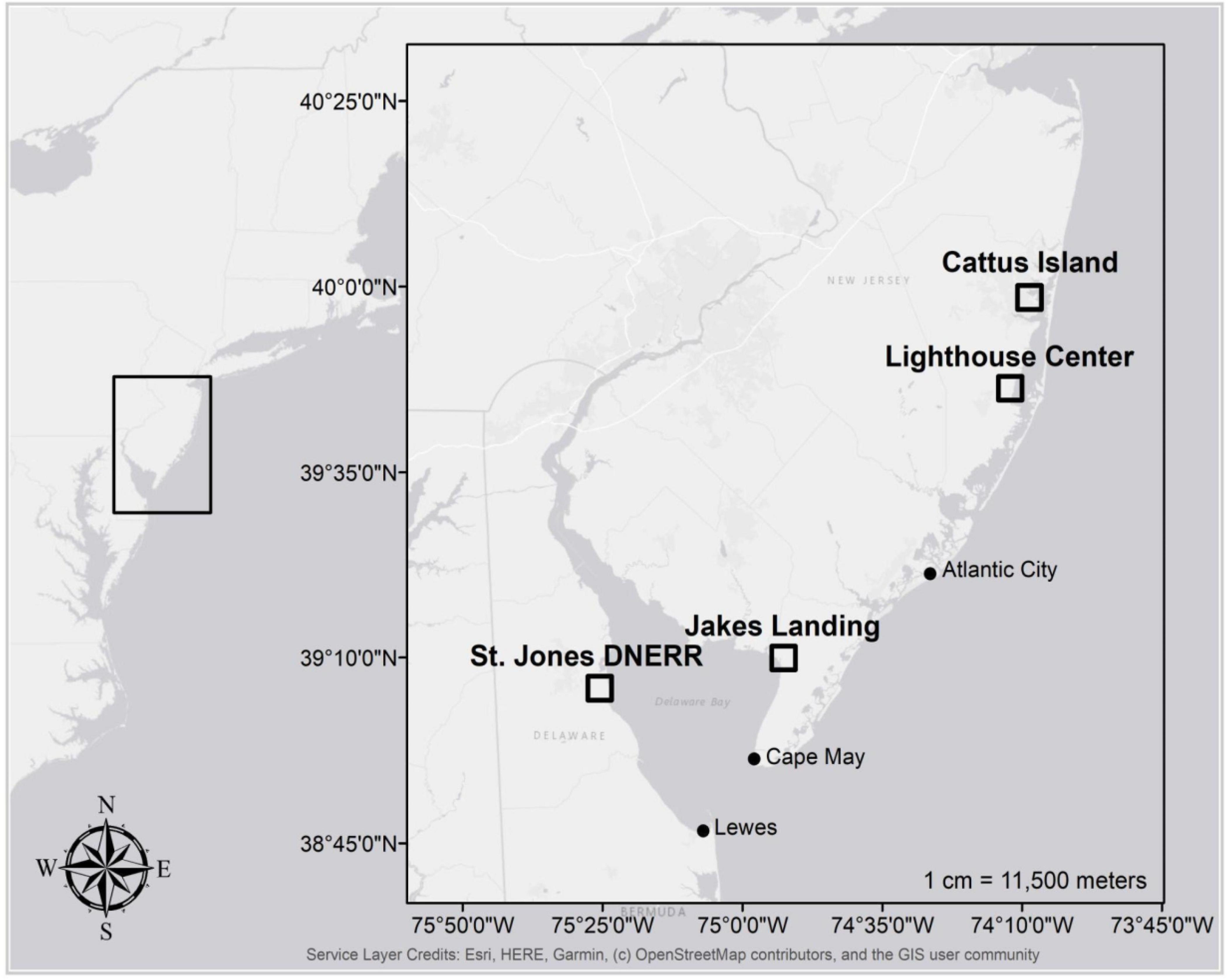
Figure 1. Map of study sites in New Jersey and Delaware (black boxes) along with the location of NOAA tide gages used to study relationships between tree growth and coastal water levels (black circles).
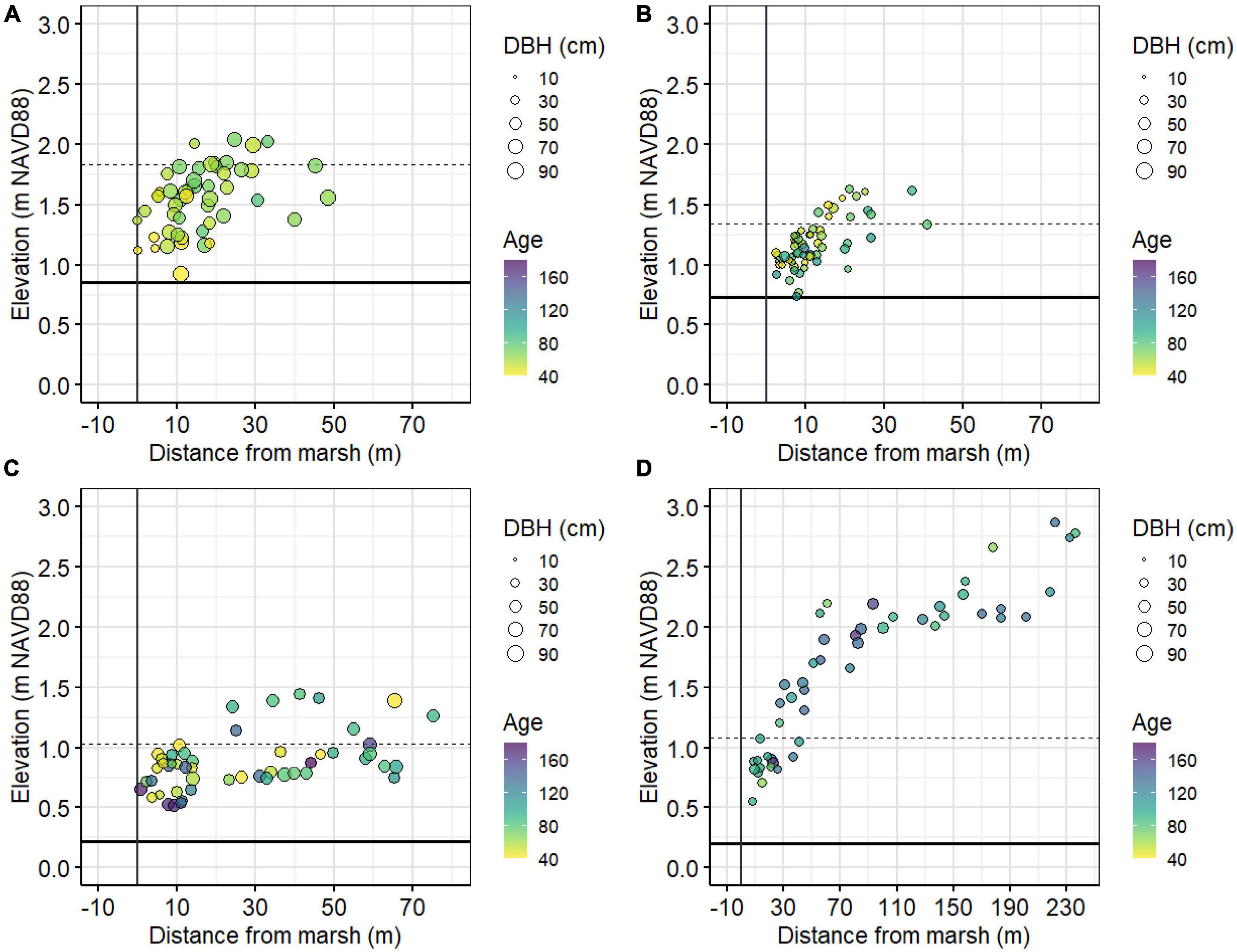
Figure 2. Graph of individual tree elevation and distance to the marsh edge for loblolly pines at Jakes Landing (A), American hollies at St. Jones (B), pitch pines at Cattus Island (C), and American hollies at the Lighthouse Center (D). Point sizes vary by diameter at breast height (DBH) and point color varies by age. Solid vertical line is the marsh edge at each site, solid horizontal line is local mean higher high water, and dashed horizontal line is the local maximum lunar tide level from ∼2000–2019.
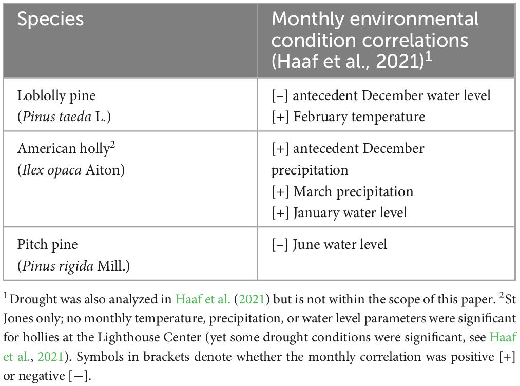
Table 1. Species description and previously published monthly environmental parameter correlations.
Across their range, loblolly and pitch pine are found where maximum temperatures are below 38°C, with pitch pines withstanding cooler minima than loblolly pines (−40°C vs. −23°C, respectively) (Burns and Honkala, 1990a). No maximum temperatures have been recorded for American holly, but minimum temperatures across the species range is −23°C (Burns and Honkala, 1990b). Cumulative annual precipitation for all three species is approximately 1,000–1,500 mm (Burns and Honkala, 1990a,b). Loblolly pines reach their most northern distribution in New Jersey, whereas American hollies reach their most northern distribution in Massachusetts. Both loblolly pine and American holly have southern distributions that extend southwest to eastern Texas. Generally, pitch pine has a more northerly distribution, from Maine to eastern Tennessee (Burns and Honkala, 1990a,b). All three species occur in an array of forest types, from mesic to xeric, across the eastern US and are common in forests abutting salt marshes in these areas.
2.2 Dendrochronological analysis
Trees cores, diameter-at-breast height, and coordinates were collected from 213 trees across the four study sites from 2018 to 2020 using standard field procedures (see Pilcher et al., 1990 for standard procedures). Tree ring widths were measured to a precision of ± 0.001 mm using a Velmex® unislide table coupled with Tellervo® measurement software. Cores were cross-dated and verified using COFECHA (Holmes, 1983). Detrended ring width indices (RWI) were derived from ring width lengths (RWL) using cubic smoothing splines, using R statistical software with the “dplR” package (Cook et al., 1990; Bunn et al., 2022; R Core Team, 2022). Detailed site descriptions, field methods, and core preparation methods are reported in Haaf et al. (2021).
2.3 Climate and water level data
Temperature and precipitation data for the study areas were obtained from the National Centers for Environmental Information (NCEI) regional climate datasets (available range from 1,895 to 2,020) (Haaf et al., 2021; Figures 3, 4). Maximum monthly water level reports from 1980 to 2020 were obtained for each National Oceanic and Atmospheric Administration (NOAA, 2020) real-time gage closest to each study site: Cape May, Lewes, and Atlantic City (NOAA, 2020; Figures 3, 4 and Supplementary Figure 2). It is important to note that these water level values were used as proxies and may not be entirely reflective of flood conditions at our coastal forest sites. For additional methods on the sourcing, derivation, and treatment of water level and climate data, see Haaf et al. (2021). On average, seasonal climatic conditions were relatively similar among sites within the relatively small latitudinal gradient (i.e., 39.089°N to 39.981°N) from 1981 to 2020 (Figure 3). Mean temperatures ranged from −0.94°C to 24.4°C with a mean of 12.5°C. Cumulative precipitation ranged from 29 to 207 mm, with a mean of 96 mm Mean maximum water levels ranged from 1.08 to 1.83 m NAVD88, with an overall mean of 1.10 m. Over the last forty years (∼1980 to present), most seasonal temperatures, precipitation, and sea level have significantly changed (Figure 4).
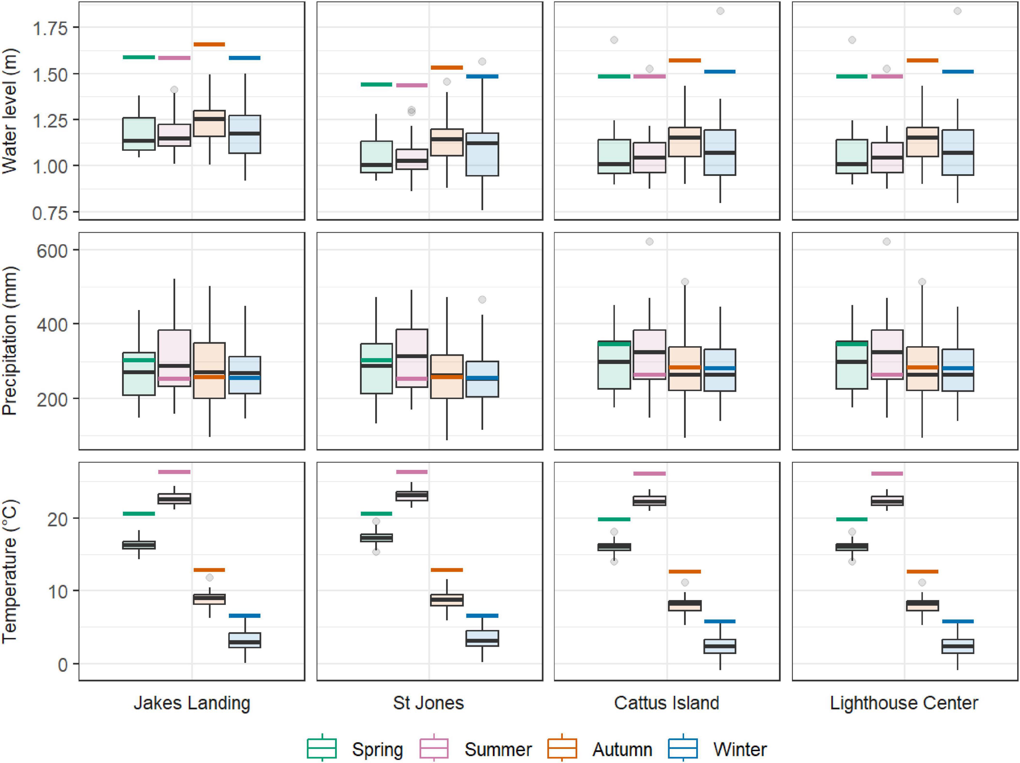
Figure 3. Boxplots of seasonal mean water level (m NAVD88, top row), cumulative precipitation (middle row), and mean temperature (bottom row) by site and species. Seasons are colored and arranged left to right: spring, summer, autumn, and winter. For each seasonal parameter, a solid colored line represents the predicted mean value for 2080.
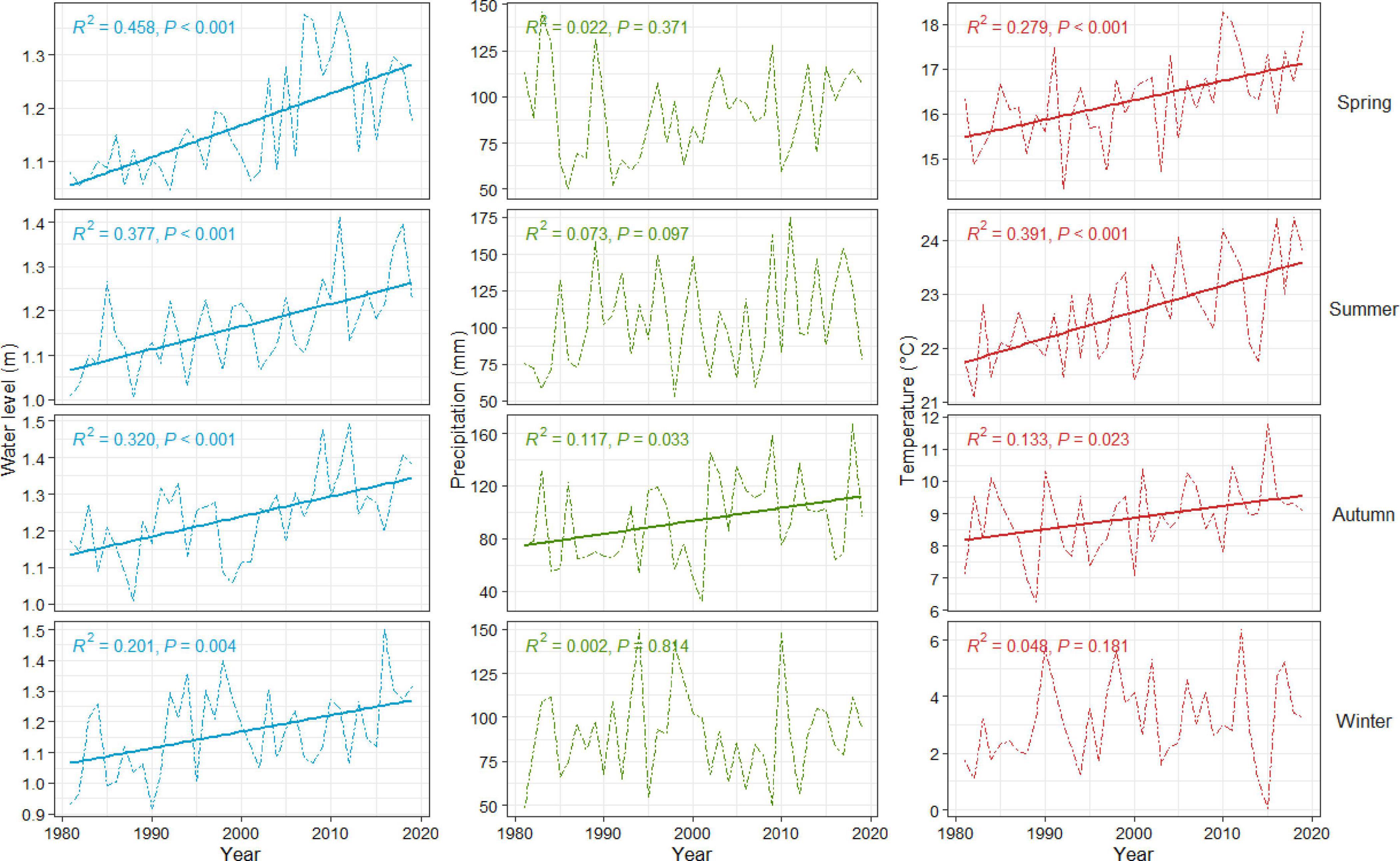
Figure 4. Seasonal trends over time in mean water level (blue, left panes), cumulative precipitation (green, center panes), and mean temperature (red, right panes) for Cape May, New Jersey (other sites follow similar patterns). Seasons are arranged top to bottom by row: spring, summer, autumn, and winter. Regression lines are provided for trends that were significant (p < 0.05).
We compared the historical distribution of temperature and precipitation from 1980 to 2019 to climate projections for 2019-2080 (Figure 3). Climate projections for Shared Socio-economic Pathways 2 (SSP2-4.5 or SSP2) from Coupled Model Intercomparison Project 6 (CMIP6) was selected because it is the intermediate greenhouse gas emissions scenario, with little change in CO2 emissions until ∼2050; other scenarios have emissions either declining or doubling (IPCC, 2023). We downloaded CMIP6 data using the Google Earth Engine CMIP6 Explorer (GEECE; Guo et al., 2018; Krasting et al., 2018; Lea et al., 2024).
Sea level projections to 2080 for a low-intermediate to intermediate climate scenario with 0.3 m global sea level rise were chosen for each NOAA tide station from Sweet et al. (2022). We added these increase values to current mean high water at each station to obtain a localized projection value. This represents a linear rise in sea level, although will likely rise exponentially through time (Callahan et al., 2017, Kopp et al., 2019, Taherkhani et al., 2020).
2.4 Statistical analyses
2.4.1 Gradient boosted regression
Gradient boosted regression trees, or gradient boosted models (GBMs), is an ensemble machine learning technique that builds a series of regressions; each new model corrects previous models by training to predict residual error. GBMs were constructed using a linear formula predicting tree ring width indices given seasonal temperature, precipitation, and maximum tidal water levels using the “gbm” package in R (R Core Team, 2022; Ridgeway et al., 2024):
Where RWI is the ring width index, T is mean seasonal temperature, P is monthly cumulative precipitation for the season, and W is mean seasonal water level. Seasons were winter (December–February); spring (March–May); summer (June–August); and autumn (September–November). Environmental parameters (T, P, and W) are denoted with the following subscripts for each season: w is winter, s is spring, u is summer, and a is autumn. All seasonal parameters were contemporaneous with the year of tree growth. GBMs were tuned with various hyperparameters, such as a shrinkage rate of 0.08, and set to stop before 1 terminal node was reached (see Supplementary Table 1 for tuning parameters used here and Bentéjac et al., 2021 for a discussion on tuning hyperparameters). GBMs were also cross-validated (nfolds = 5, random splits).
Growth optima can be interpreted through single-variable partial dependence plots (PDPs; Greenwell, 2017) by discerning where the response variable (i.e., RWI) is maximized along the parameter gradient (Lloyd et al., 2013; Gu et al., 2019). PDPs show predicted RWI (ŷ) for each seasonal parameter within the GBM (Equation 1). Both linear regressions and generalized additive models (GAM) of GBM model outputs were then used to discern and visualize how growth responses varied as parameter values changed (for GAMs, we used “mgcv” and “ggplot2” packages in R; Wood, 2011; Wickham, 2016). GBM modeled RWI values (i.e., ŷ) were compared to current (1979–2019) seasonal summaries of temperature, precipitation, and tidal water levels to discern whether existing conditions fell below, met, or exceeded model-derived optima. Finally, we compared current averages to climate and sea level projections for the next ∼60 years (see section 2.3 “Climate and water level data”) relative to modeled growth response to see how climate change will affect growth predictions for species at each site.
2.4.2 Backward elimination and generalized additive models
In addition to comparisons with the previous correlation study on each site’s mean chronology (i.e., Haaf et al., 2021), here we ran traditional statistical tests on the relationships among climate variables, water levels, and tree ring width to help contextualize GBM results. We first built several linear mixed models consisting of raw RWLs with individual trees as random effects and year, seasonal mean temperature, cumulative precipitation, and mean maximum tidal water as fixed effects. We used backward log-likelihood stepwise elimination to simplify these models and identify which variables were likely the best linear parameters of current tree growth using the “buildmer,” “lme4,” and “MuMIn” packages in R (Bates et al., 2015; Voeten, 2022; Bartoń, 2023).
Next, we constructed pairwise interaction-only GAMs for each site using the “mgcv” package in R (Wood, 2011). Each GAM model accounted for individual trees and grouped two-way relationships by season (i.e., no interactions among seasons were tested). These GAM results were then used to identify which pairs had significant (α = 0.05) smoother terms and if those relationships were linear (effective degrees of freedom, or edf = 1) or non-linear (edf > 1). Although GBMs were run on RWI, similar to previous correlation studies, these additional tests were run on RWLs of individual trees to account for tree-specific variation.
3 Results
3.1 Model fits
3.1.1 Gradient boosted regression
GBM test set accuracy results ranged from 82 to 97% and root mean square errors (RMSE) ranged from 0.128 to 0.271 mm (Supplementary Table 1). Relationships between loblolly pine RWI and environmental variables at Jakes Landing had the lowest RMSEs among the sites (∼0.12 units RWI), whereas American hollies at St Jones was highest (∼0.25 units RWI). Relationships between environmental conditions and pitch pine RWI at Cattus Island and American holly RWI at the Lighthouse Center had RMSEs of about ∼0.20 mm across all models (Supplementary Table 1).
Of the 48 linear models used to discern trends in GBM-modeled RWI with seasonal environmental parameters (i.e., PDP results), 35 tests were statistically significant (73%; < 0.05) (Figures 5–8). At Jakes Landing, regressions of modeled RWI in PDPs suggest that modeled RWI significantly increased with increasing water levels in spring, summer, and autumn, but decreased with increasing water levels in winter (Figure 5). Modeled RWI also significantly increased with increasing spring and winter precipitation. For temperature, modeled RWI significantly increased with spring, summer, and winter temperatures, but decreased with warmer autumn temperatures. For American hollies at St Jones, modeled RWI significantly decreased with increasing water levels in summer but increased with increasing water levels in winter (Figure 6). Modeled RWI also significantly increased with increasing precipitation across spring, summer, and autumn, but RWI decreased with increasing winter precipitation. Modeled RWI significantly increased with spring and summer temperature but decreased with increasing winter temperatures.
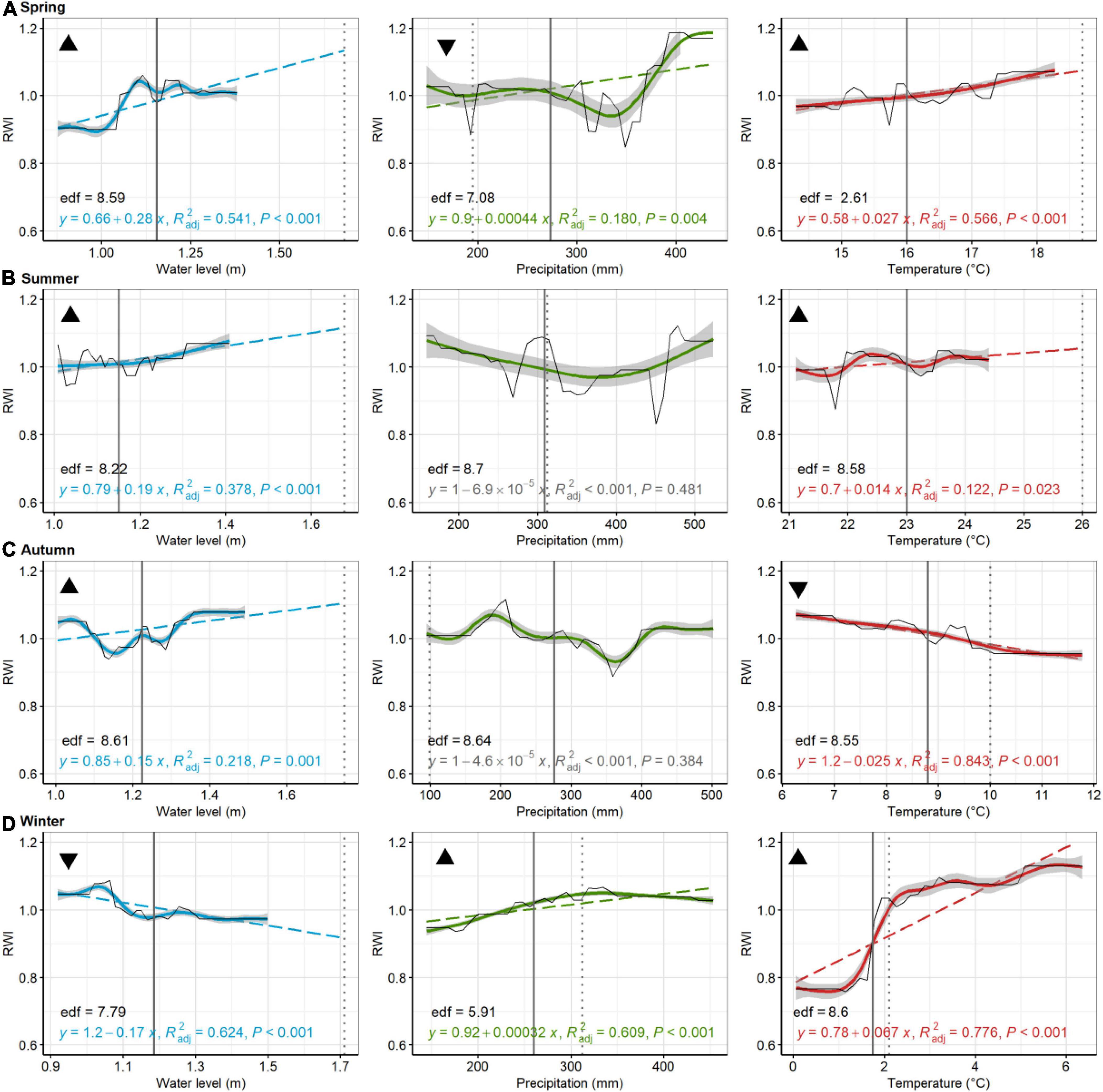
Figure 5. Loblolly pine, Jakes Landing. Partial dependence plots of model-fitted RWI for seasonal [spring, (A); summer, (B); autumn, (C); and winter, (D)] water level, precipitation, and temperature. Black lines are means of cross-validated models (also see Supplementary Figure 3). Dashed trend lines are linear regressions shown when p < 0.05. Linear regression results, shown in color (in gray if p > 0.05), consist of the model equation, adjusted R2, and p-value. Curvilinear trends, with gray 95% confident boundaries, are fitted with a generalized additive model (GAM). GAM effective degrees of freedom (edf) are shown in black. Solid vertical lines are current means (1980–2019) for each environmental variable, whereas broken lines are the 2080 projected value for precipitation, temperature, and water levels. Triangular symbols in the upper left of each pane represent whether RWI trends for each seasonal parameter suggest more (upward triangle) or less (downward triangle) growth as the climate changes or sea levels rise. Panes without these symbols show which comparisons were inconclusive, based on lack of linear trends in growth or because the environmental parameter has minimal predicted change.
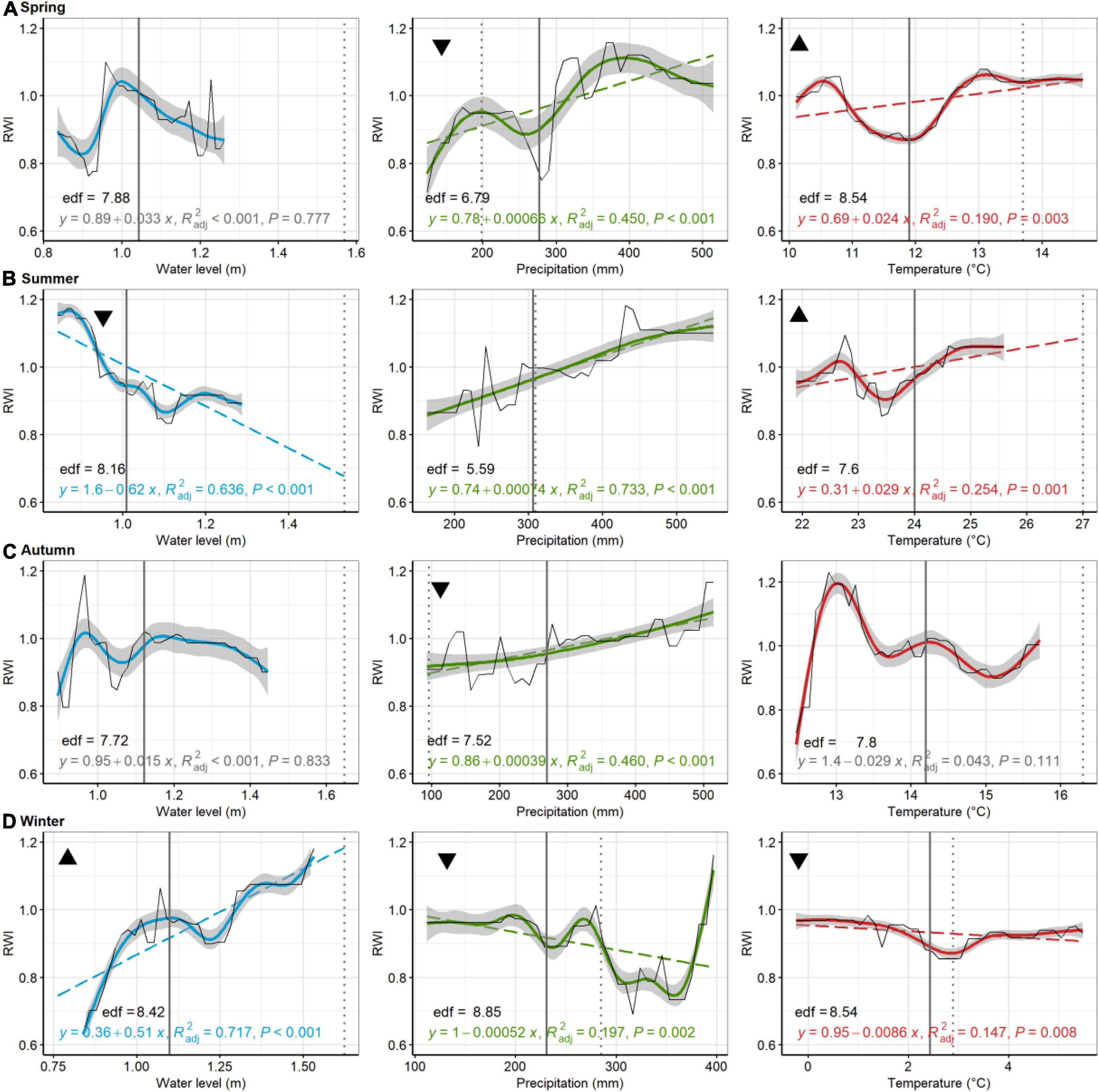
Figure 6. American holly, St Jones. Partial dependence plots of model-fitted RWI for seasonal [spring, (A); summer, (B); autumn, (C); and winter, (D)] water level, precipitation, and temperature. Black lines are means of cross-validated models (also see Supplementary Figure 4). Dashed trend lines are linear regressions shown when p < 0.05. Linear regression results, shown in color (in gray if p > 0.05), consist of the model equation, adjusted R2, and p-value. Curvilinear trends, with gray 95% confident boundaries, are fitted with a generalized additive model (GAM). GAM effective degrees of freedom (edf) are shown in black. Solid vertical lines are current means (1980–2019) for each environmental variable, whereas broken lines are the 2080 projected value for precipitation, temperature, and water levels. Triangular symbols in the upper left of each pane represent whether RWI trends for each seasonal parameter suggest more (upward triangle) or less (downward triangle) growth as the climate changes or sea levels rise. Panes without these symbols show which comparisons were inconclusive, based on lack of linear trends in growth or because the environmental parameter has minimal predicted change.
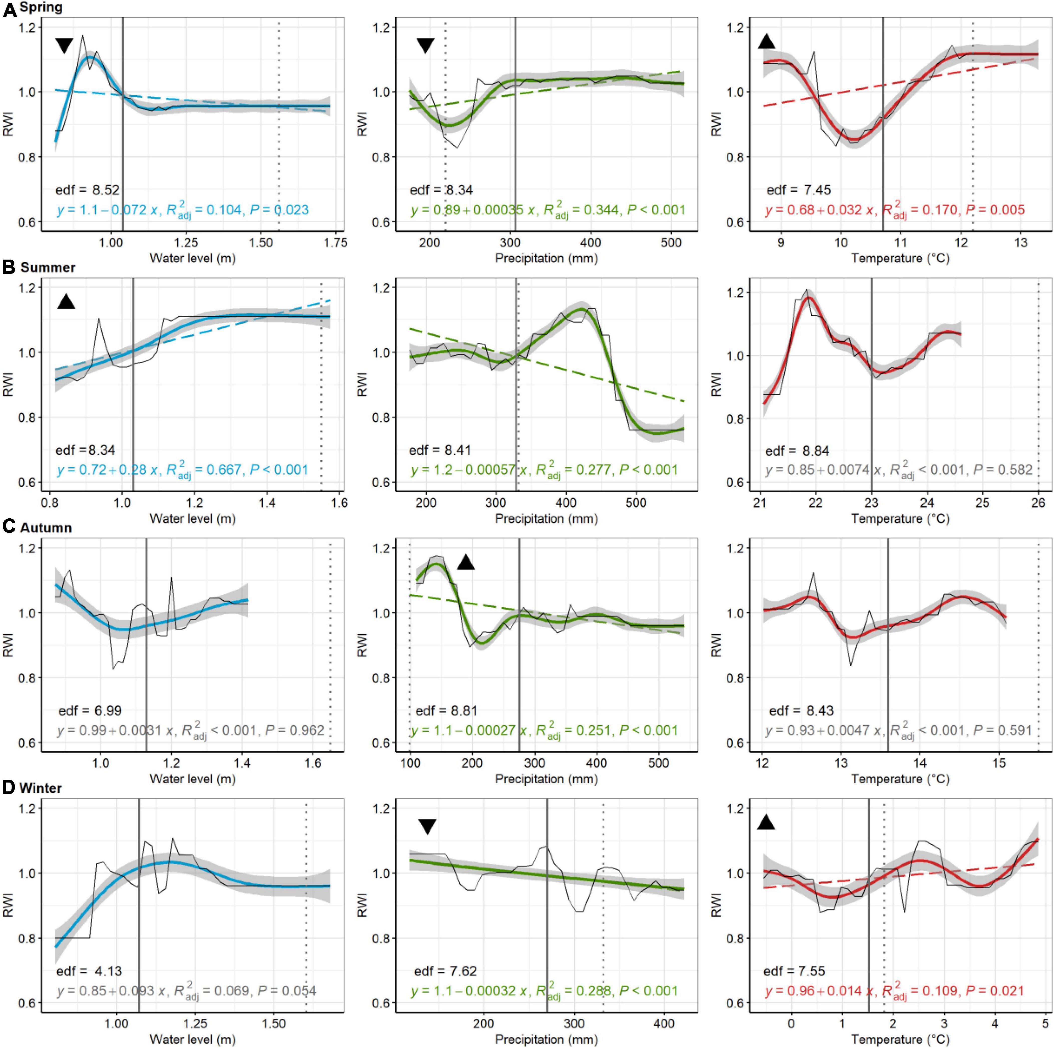
Figure 7. Pitch pine, Cattus Island. Partial dependence plots of model-fitted RWI for seasonal [spring, (A); summer, (B); autumn, (C); and winter, (D)] water level, precipitation, and temperature. Black lines are means of cross-validated models (also see Supplementary Figure 5). Dashed trend lines are linear regressions shown when p < 0.05. Linear regression results, shown in color (in gray if p > 0.05), consist of the model equation, adjusted R2, and p-value. Curvilinear trends, with gray 95% confident boundaries, are fitted with a generalized additive model (GAM). GAM effective degrees of freedom (edf) are shown in black. Solid vertical lines are current means (1980–2019) for each environmental variable, whereas broken lines are the 2080 projected value for precipitation, temperature, and water levels. Triangular symbols in the upper left of each pane represent whether RWI trends for each seasonal parameter suggest more (upward triangle) or less (downward triangle) growth as the climate changes or sea levels rise. Panes without these symbols show which comparisons were inconclusive, based on lack of linear trends in growth or because the environmental parameter has minimal predicted change.
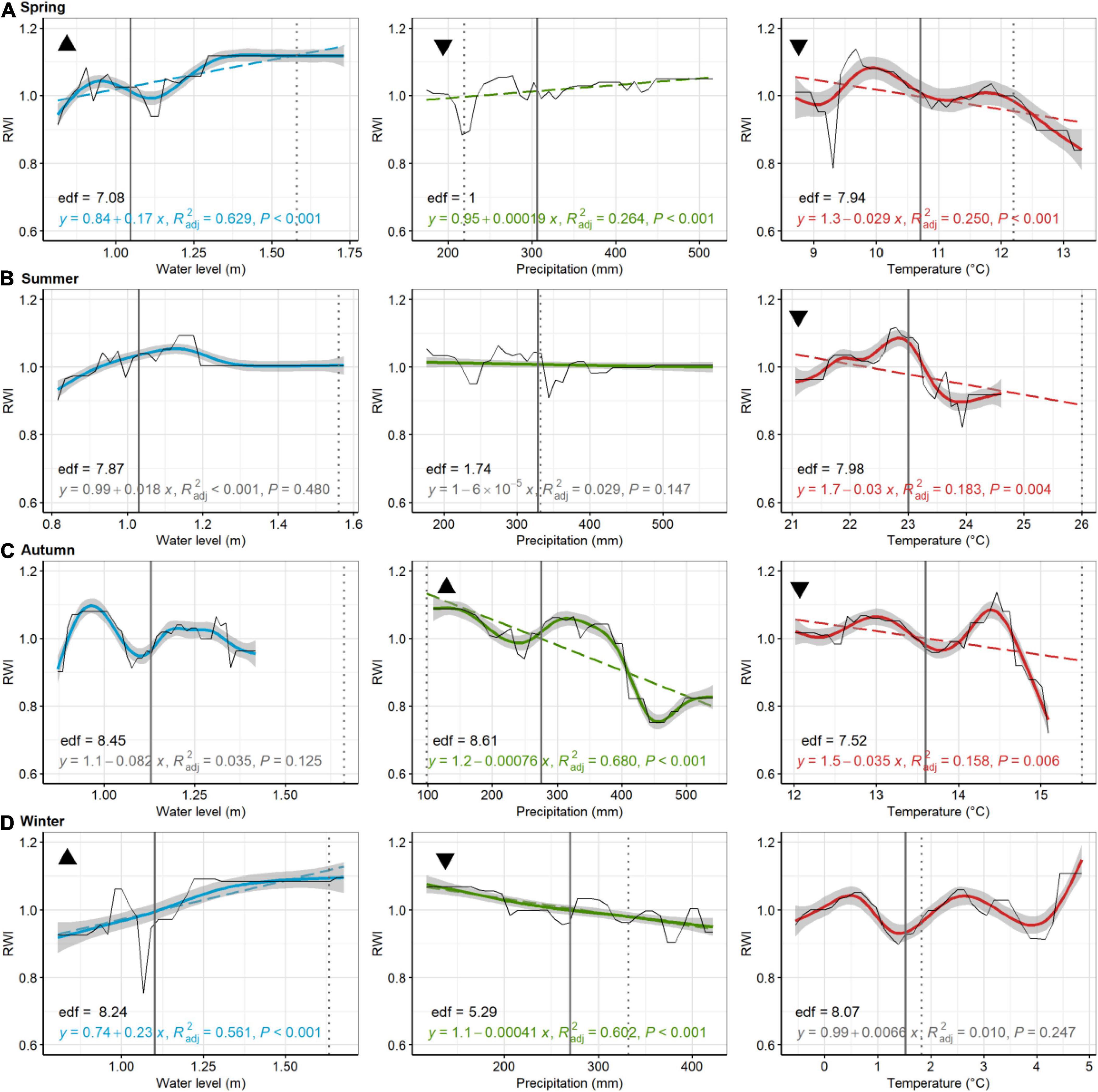
Figure 8. American holly, Lighthouse Center. Partial dependence plots of model-fitted RWI for seasonal [spring, (A); summer, (B); autumn, (C); and winter, (D)] water level, precipitation, and temperature. Black lines are means of cross-validated models (also see Supplementary Figure 6). Dashed trend lines are linear regressions shown when p < 0.05. Linear regression results, shown in color (in gray if p > 0.05), consist of the model equation, adjusted R2, and p-value. Curvilinear trends, with gray 95% confidence boundaries, are fitted with a generalized additive model (GAM; not shown if effective degrees of freedom (edf) = 1). GAM edf are shown in black. Solid vertical lines are current means (1980–2019) for each environmental variable, whereas broken lines are the 2080 projected value for precipitation temperature, and water levels. Triangular symbols in the upper left of each pane represent whether RWI trends for each seasonal parameter suggest more (upward triangle) or less (downward triangle) growth as the climate changes or sea levels rise. Panes without these symbols show which comparisons were inconclusive, based on lack of linear trends in growth or because the environmental parameter has minimal predicted change.
At Cattus Island, modeled pitch pine modeled RWI significantly increased with increasing summer water levels, but decreased with increasing spring water levels (Figure 7). Modeled RWI decreased with increasing summer, autumn, and winter precipitation but increased with increasing spring precipitation. Modeled RWI increased with increasing spring and winter temperatures. For American hollies at the Lighthouse Center, modeled RWI significantly increased with increasing spring and winter water levels (Figure 8). Modeled RWI significantly increased with increasing spring precipitation but decreased with increasing autumn and winter precipitation. Modeled RWI significantly decreased with spring, summer, and autumn temperatures.
3.1.2 Backward elimination and generalized additive models
Backward elimination of linear models suggested several possibly important environmental parameters of tree growth for both locations in the Delaware Bay (Table 2). Individual trees accounted for 62% of the model variance at Jakes Landing and 31% of the variance at St Jones. Marginal R2 (i.e., fixed without random effects) values for Jakes Landing and St Jones were 0.0266 and 0.0826, respectively; conditional R2 (i.e., with random and fixed effects) values for Jakes Landing and St Jones were 0.633 and 0.368, respectively. Backward elimination suggested intercept-only models for both Barnegat Bay sites, so no parameters were identified for a good model fit (Table 2).
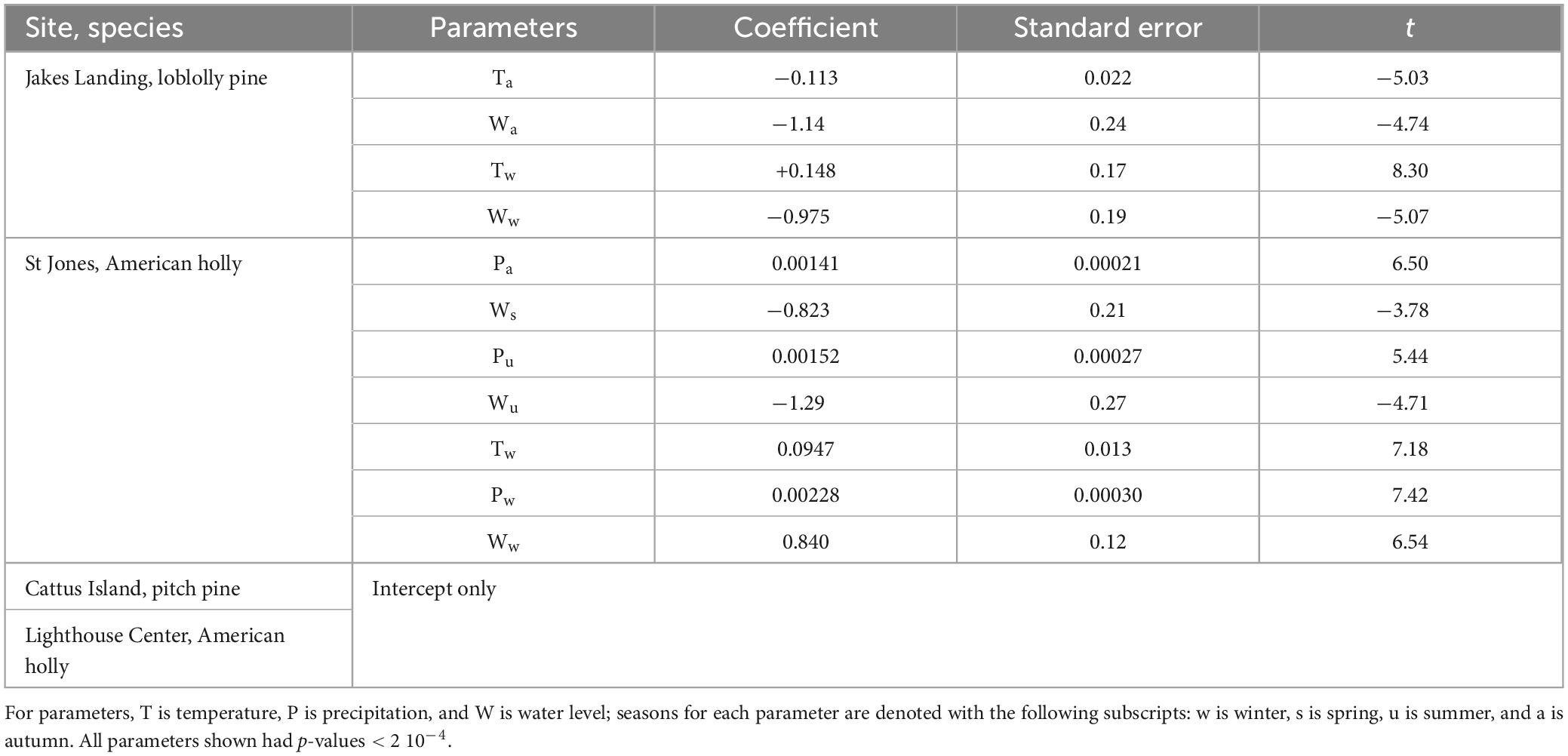
Table 2. Linear mixed models results from backward elimination.
GAM results for single parameters explained a large portion of deviance at all sites (60–97%), with all tests, except for spring precipitation for American holly at the Lighthouse Center, suggesting important non-linear smoothers for model fit (Figures 5–8). Additionally, pairwise interaction term GAMs suggest that, 32 of the 48 tests (66%) had represented a significant interaction (α < 0.05) and 26 of those 32 significant tests were non-linear (81%; edf > 1) (Table 3).

Table 3. Two-way interaction generalized additive models.
3.2 Climate change and tree growth
Climate change predictions varied across seasons (Figure 3), and coupled with already observed trends in these parameters (Figure 4), represent considerable possible changes to growth capacity in these coastal forests. Predictions for precipitation were similar to current autumn and winter levels, but spring projections were typically higher, and summer lower, than the current the means. Predictions for temperature and water levels were higher for all seasons. These predictions mostly corroborate trends observed over the last 40 years, except for precipitation, which tends to have higher variability that limits finding significant trends over time, and spring temperatures, which have been increasing despite predictions of cooling.
In comparing trends in growth variation across each seasonal parameter with predicted climate or water level change (see black triangles in Figures 5–8), patterns emerged that suggested tree growth might be affected positively or negatively by predicted changes. At Jakes Landing, loblolly pine growth might increase due to warmer springs, summers, and winters, wetter winters (i.e., increased precipitation), and higher spring, summer, or autumn water levels, yet decrease due to warmer autumns, drier springs and increasing winter water levels (Figure 5). For American holly at St Jones, growth may increase due to warmer springs and summers, as well as increasing winter water levels, but decrease in response to drier springs and autumns, wetter winters, increased summer water levels, and warmer winter temperatures (Figure 6). For Cattus Island, pitch pine growth may increase due to warmer springs and winters, increasing summer water levels, and drier autumns, yet growth may decrease in response to drier springs and wetter winters, and increased spring water levels (Figure 7). American holly at the Lighthouse Center may experience increased growth due to increased water levels in spring and winter, as well as drier autumns, yet grow less in response to drier springs, wetter winters, and warmer springs, summers, and autumns (Figure 8).
4 Discussion
The mortality and retreat of coastal forests in response to climate change and sea levels rise will shape future coastal landscapes. Although slope likely plays a fundamental role in how quickly forests are affected by rising sea levels (Smith, 2013; Schieder et al., 2018; Molino et al., 2021), the variability of rates in moderate to low slope environments suggest that ecological or site-specific characteristics are important factors in retreat (Fagherazzi et al., 2019; Powell et al., 2024). One likely component of this variability is how different tree species respond to changing environmental conditions, which can be discerned through tree ring patterns (Fritts, 1978). As temperatures rise, precipitation changes, and flood frequency increases (Figures 3, 4), studying tree rings to understand growth responses to environmental conditions can help managers foreshadow how coastal forests may fare into the future. As a first step, this study sought to examine how tree growth varies with environmental conditions (i.e., climate, tidal flooding) and infer the effects of changing conditions on the vulnerability for tree species common in the low-lying coastal forests in New Jersey and Delaware to future mortality.
Higher water levels are generally thought to reduce tree growth and these results suggested that while this might be the case occasionally, positive associations between RWI and water levels were detected regularly (e.g., Ww for American holly at St Jones, Table 2; Figures 5A–C, 6D, 7B, 8A, D). Other recent studies have also found mixed growth responses to increased saltwater flood exposure (Field et al., 2016; Haaf et al., 2021; Noe et al., 2021). One possible mechanism is that conditions that correlate with tidal water levels, like groundwater levels, could have regular influence on tree growth within these coastal forest systems. As an example, higher tide levels elevate groundwater tables and could enhance moisture availability during times of low precipitation (e.g., via hydraulic lift; Dawson, 1996). Groundwater has been shown to subsidize tree growth in sandy soils (Ciruzzi and Loheide, 2021), which are common in the coastal plains of New Jersey and Delaware (Markewich et al., 1990). How these conditions affect tree growth within a broader geographical scale, however, is unclear (see local case studies by Hirano et al., 2018; Kearney et al., 2019; Wang et al., 2020; Ross et al., 2021) and more research is needed to make predictions at the landscape level. Another possible explanation is that during high water events, trees may not be directly flooded or may not be flooded long enough to elicit detectable responses, especially if floods last less than a few hours or days. Trees might evade short-term flood damage by closing stomata, with damage taking days to develop (e.g., anaerobic conditions; Kozlowski, 1982). Importantly, our analyses here look only at contemporaneous conditions within the year of tree growth, but it is highly likely that growth effect lags exist with previous conditions, such that future studies should consider previous months, seasons, or even years to elucidate possible relationships.
Gradient boosting regression models in this study suggested that seasonal conditions and their predicted changes have varied consequences on growth (Figures 5–8). Changes across a parameter gradient could be detrimental or beneficial to trees depending on growth responses (Lloyd et al., 2013; Gu et al., 2019). For instance, results for Jakes Landing loblolly pine here show a strong increase in growth with increasing winter temperatures (Figure 5D), which mirrors results from linear mixed models (Table 2) and previous correlation studies (Table 1; Haaf et al., 2021). Especially as its most northern distribution, warming winters will likely have positive effects on loblolly pine growth given strong positive correlations with winter temperatures. Loblolly ring widths, however, may decrease with warmer autumns (Figures 3, 4, 5C). Warmer autumn temperatures may interfere with latewood production if temperatures drop abruptly thereafter (Piermattei et al., 2015; Begum et al., 2018), potentially leading to higher cavitation vulnerability in the winter (Pereira et al., 2018). This, in turn, may exacerbate vulnerability to higher winter water levels thereafter (Figure 5D).
GBM results further showed that non-linear relationships existed between growth and environmental parameters for most sites and species (Figures 5–8 and Table 3). For instance, both American holly at St Jones and pitch pines at Cattus Island have non-linear responses to spring temperatures, where growth reaches minima at mid-temperature ranges (∼10 or 11°C) (Figures 7, 8). On occasion, multiple extrema even suggest that some relationships could be multi-nodal (e.g., holly growth relative to spring precipitation at St Jones, Figure 6A). Although linear mixed models match GMB output for Jakes Landing loblolly pine, non-linearity could be why linear mixed model and GBM results were not entirely congruent at St Jones. At St Jones, American holly had four significant linear model coefficients (autumn and summer precipitation; summer and winter water levels) that matched GBM results. Yet, the other four parameters either had non-significant linear relationships (i.e., autumn temperature, Figure 6C, and spring water levels, Figure 6A) or GBM concurred that the parameter was significant but directionality was opposite (i.e., winter temperature and winter precipitation, Figure 6D). In these four examples, GAM results suggest a high degree of non-linearity (where edf > 7.5). Secondly, linear mixed models generally failed for sites in Barnegat Bay and non-linearity may be the culprit. GBM, in these instances, can provide insight into relationships that linear tests might not be able to detect. Parameters that suggest opposing results for different statistical tests require more study to understand these relationships more definitively. Regardless, non-linear and/or multi-modal relationships have also been found in previous tree ring studies (Lloyd et al., 2013; Gu et al., 2019; Matisons et al., 2021; Anderson-Teixeira et al., 2022). Ultimately, non-linear relationships suggest biological or ecological complexities exist that require further study (e.g., Rossi et al., 2013).
Site-specific responses to climate and flooding conditions could be one of the likely leading mechanisms of variability in forest retreat relative to rising sea levels. Site-specificity has received recent focus in attempting to understand drought mortality (Trugman et al., 2021). This study analyzed tree rings from three species at four sites, across two estuarine settings, yet we could not make generalizations about species- or estuary-specific patterns of tree growth across environmental gradients. American holly growth at the Lighthouse Center, for example, decreased significantly with increasing autumn precipitation whereas holly growth at St Jones increased (Figures 6B, 8B, respectively). Hypothetically, hollies at the Lighthouse Center could be generally more vulnerable to mortality during stormy and wet autumns even though hollies St Jones likely have higher flood exposures in general (i.e., lower elevations, Figure 2; Haaf et al., 2021). A single large storm surge event during a wet autumn might be particularly detrimental for hollies at the Lighthouse Center if seasonal temperatures climb and precipitation had already waterlogged roots, which may occur more frequently as autumn precipitation increases (Figure 4).
Following Liebig’s Law, sensitivity to seasonal conditions might vary for the same species at different locations depending on site-specific limiting factors, such as nutrient or moisture availability (Stine and Huybers, 2017; Stine, 2019). Topography, soil types, forest structure (e.g., tree size/age classes, density) or composition (e.g., species dominance), and flood or meteorological exposure (Carr et al., 2020), could all also instill limitations on resources and influence stress gradients. Interactions with site-specific conditions, many of which may be non-linear, likely predispose different coastal forests to stress in unique ways which complicates predicting where or when coastal forests retreat as sea levels rise.
5 Conclusion
Retreating coastal forests is a primary consequence of rising sea levels, but regional variability in rates of retreat make predicting where and how quickly forest loss will occur difficult. Patterns in tree growth, as a proxy for stress and mortality vulnerability, showed that relationships with climate and tidal flooding are complex and frequently non-linear. As climates change, and sea levels rise, some sites or species may confer benefits to growth, whereas other sites may experience conditions that reduce growth. Site-specificity of results underscores the importance of local conditions on tree growth in coastal forests. To aid future management efforts, future research should examine site-specific mechanisms and explore non-linear relationships that may contribute to tree responses to climate and tidal flooding.
Data availability statement
The original contributions presented in this study are included in this article/Supplementary material, further inquiries can be directed to the corresponding author.
Author contributions
LH: Conceptualization, Data curation, Formal analysis, Investigation, Methodology, Visualization, Writing – original draft, Writing – review & editing. SD: Conceptualization, Funding acquisition, Supervision, Writing – review & editing.
Funding
The authors declare that financial support was received for the research, authorship, and/or publication of this article. This work was partially supported by a private donation to the Susan Kilham Research Fund.
Acknowledgments
We are grateful to Susan S. Kilham, Elizabeth B. Watson, Danielle A. Kreeger, and David J. Velinsky for their advisement on this study. We are also thankful for the support of those who helped in the field. We are also appreciative for field site access granted by New Jersey Fish and Wildlife, the Delaware National Estuarine Research Reserve, and Cattus Island County Park.
Conflict of interest
LH was employed by Partnership for the Delaware Estuary Inc.
The remaining author declares that the research was conducted in the absence of any commercial or financial relationships that could be construed as a potential conflict of interest.
Publisher’s note
All claims expressed in this article are solely those of the authors and do not necessarily represent those of their affiliated organizations, or those of the publisher, the editors and the reviewers. Any product that may be evaluated in this article, or claim that may be made by its manufacturer, is not guaranteed or endorsed by the publisher.
Supplementary material
The Supplementary Material for this article can be found online at: https://www.frontiersin.org/articles/10.3389/ffgc.2024.1362650/full#supplementary-material
References
Anderson-Teixeira, K. J., Herrmann, V., Rollinson, C. R., Gonzalez, B., Gonzalez-Akre, E. B., Pederson, N., et al. (2022). Joint effects of climate, tree size, and year on annual tree growth derived from tree-ring records of ten globally distributed forests. Glob. Change Biol. 28, 245–266. doi: 10.1111/gcb.15934
Bartoń, K. (2023). “MuMIn: Multi-model inference”. R package version 1.47.5. Available online at: https://CRAN.R-project.org/package=MuMIn
Bates, D., Maechler, M., Bolker, B., and Walker, S. (2015). Fitting linear mixed-effects models using lme4. J. Stat. Softw. 67, 1–48. doi: 10.18637/jss.v067.i01
Begum, S., Kudo, K., Rahman, M. H., Nakaba, S., Yamagishi, Y., Nabeshima, E., et al. (2018). Climate change and the regulation of wood formation in trees by temperature. Trees Struct. Funct. 32, 3–15. doi: 10.1007/s00468-017-1587-6
Bentéjac, C., Csörgő, A., and Martínez-Muñoz, G. (2021). A comparative analysis of gradient boosting algorithms. Artif. Intell. Rev. 54, 1937–1967.
Bigler, C., and Bugmann, H. (2004). Predicting the time of tree death using dendrochronological data ecological applications. 14, 902–914.
Bunn, A., Korpela, M., Biondi, F., Campelo, F., Mérian, P., Qeadan, F., et al. (2022). dplR: Dendrochronology program library in R. R package version 1.7.4. Available online at: https://CRAN.R-project.org/package=dplR
Burns, R. M., and Honkala, B. H. (1990a). Volume 1: Conifers. Silvics of North America. Vol. 1. Washington, DC: US Department of Agriculture, Forest Service, doi: 10.2307/j.ctt1ffjhpb.19
Burns, R. M., and Honkala, B. H. (1990b). Volume 2: Hardwoods. Silvics of North America - Volume 2, Hardwoods 2. Washington, DC: US Department of Agriculture, Forest Service, 148–152.
Butler-Leopold, P. R., Iverson, L. R., Thompson, F. R. III, Brandt, L. A., Handler, S. D., Janowiak, M. K., et al. (2018). Mid-Atlantic forest ecosystem vulnerability assessment and synthesis: A report from the mid-Atlantic climate change response framework project. Newtown Square, PA: U.S. Department of Agriculture, Forest Service, Northern Research Station.
Callahan, J. A., Horton, B. P., Nikitina, D. L., Sommerfield, C. K., McKenna, T. E., and Swallow, D. (2017). Recommendation of sea-level rise planning scenarios for delaware: Technical report, prepared for Delaware department of natural resources and environmental control (DNREC) Delaware coastal programs. Newark, DE: Delaware Geological Survey.
Carr, J., Guntenspergen, G., and Kirwan, M. (2020). Modeling marsh-forest boundary transgression in response to storms and sea-level rise. Geophys. Res. Lett. 47:8998. doi: 10.1029/2020GL088998
Chen, Y., and Kirwan, M. L. (2022). Climate-driven decoupling of wetland and upland biomass trends on the mid-Atlantic coast. Nat. Geosci. 15, 913–918.
Chen, Y., and Kirwan, M. L. (2023). Upland forest retreat lags behind sea-level rise in the mid-Atlantic coast. Glob. Change Biol. 30:e17081.
Ciruzzi, D. M., and Loheide, S. P. (2021). Groundwater subsidizes tree growth and transpiration in sandy humid forests. Ecohydrology 14:e2294. doi: 10.1002/eco.2294
Cook, E., Briffa, K., Shiyatov, S., Mazepa, V., and Jones, P. D. (1990). “Data analysis,” in Methods of dendrochronology, eds E. R. Cook and L. A. Kairiukstis (Dordrecht: Springer), doi: 10.1007/978-94-015-7879-0_3
Dawson, T. E. (1996). Determining water use by trees and forests from isotopic, energy balance and transpiration analyses: The roles of tree size and hydraulic lift. Tree Physiol. 16, 263–272. doi: 10.1093/treephys/16.1-2.263
Dormann, C. F., Elith, J., Bacher, S., Buchmann, C., Carl, G., Carré, G., et al. (2013). Collinearity: A review of methods to deal with it and a simulation study evaluating their performance. Ecography 36, 27–46.
Dupigny-Giroux, L. A., Mecray, E. L., Hodgkins, G. A., Lemcke-Stampone, M. D., Lentz, E. E., Mills, K. E., et al. (2018). “. Northeast,” in Proceedings of the impacts, risks, and adaptation in the United States: 4th national climate assessment, eds D. R. Reidmiller, C. W. Avery, D. R. Easterling, K. E. Kunkel, K. L. M. Lewis, T. K. Maycock, et al. (Washington, DC: U.S. Global Change Research Program), 669–742. doi: 10.7930/NCA4.2018.CH18
Elith, J., Leathwick, J. R., and Hastie, T. (2008). A working guide to boosted regression trees. J. Anim. Ecol. 77, 802–813. doi: 10.1111/j.1365-2656.2008.01390.x
Fagherazzi, S., Anisfeld, S. C., Blum, L. K., Long, E. V., Feagin, R. A., Fernandes, A., et al. (2019). Sea level rise and the dynamics of the marsh-upland boundary. Front. Environm. Sci. 7:25. doi: 10.3389/fenvs.2019.00025
Fanelli, C., Fanelli, P., and Wolcott, D. (2013). NOAA water level and meteorological data report—Hurricane Sandy. Silver Spring, MD: US Department of Commerce, National Oceanic and Atmospheric Administration, National Ocean Service Center for Operational Oceanographic Products and Services.
Fang, K., Frank, D., Zhao, Y., Zhou, F., and Seppä, H. (2015). Moisture stress of a hydrological year on tree growth in the Tibetan Plateau and surroundings. Environ. Res. Lett. 10:034010.
Field, C. R., Gjerdrum, C., and Elphick, C. S. (2016). Forest resistance to sea-level rise prevents landward migration of tidal marsh. Biol. Conserv. 201, 363–369.
Fritts, H. C. (1978). Tree rings, a record of seasonal variations in past climate. Naturwissenschaften 65, 48–56. doi: 10.1007/BF00420633
Greenwell, B. M. (2017). pdp: An R package for constructing partial dependence plots. R J. 9, 421–436. doi: 10.32614/rj-2017-016
Gu, H., Wang, J., Ma, L., Shang, Z., and Zhang, Q. (2019). Insights into the BRT (boosted regression trees) method in the study of the climate-growth relationship of Masson pine in subtropical China. Forests 10, 1–20. doi: 10.3390/f10030228
Guo, H., John, J. G., Blanton, C., McHugh, C., Nikonov, S., Radhakrishnan, A., et al. (2018). NOAA-GFDL GFDL-CM4 model output. Earth Syst. Grid Fed. 25:1402. doi: 10.22033/ESGF/CMIP6.1402
Haaf, L., Dymond, S. F., and Kreeger, D. A. (2021). Principal factors influencing tree growth in low-lying mid Atlantic coastal forests. Forests 12, 1–18. doi: 10.3390/f12101351
Hall, S., Stotts, S., and Haaf, L. (2022). Influence of climate and coastal flooding on eastern red cedar growth along a marsh-forest ecotone. Forests 13:862. doi: 10.3390/f13060862
Hirano, Y., Todo, C., Yamase, K., Tanikawa, T., Dannoura, M., Ohashi, M., et al. (2018). Quantification of the contrasting root systems of Pinus thunbergii in soils with different groundwater levels in a coastal forest in Japan. Plant Soil 286, 1–11. doi: 10.1007/s11104-018-3630-9
Holmes, R. (1983). Computer-assisted quality control in tree-ring dating and measurement. Tree Ring Bull. 35, 41–47.
IPCC (2023). “Sections,” in Proceedings of the climate change 2023: Synthesis report: Contribution of working groups I, II and III to the 6th assessment report of the intergovernmental panel on climate change, eds H. Lee and J. Romero (Geneva: IPCC), 35–115. doi: 10.59327/IPCC/AR6-9789291691647
Kearney, W. S., Fernandes, A., and Fagherazzi, S. (2019). Sea-level rise and storm surges structure coastal forests into persistence and regeneration niches. PLoS One 14:18–20. doi: 10.1371/journal.pone.0215977
Kirwan, M. L., Kirwan, J. L., and Copenheaver, C. A. (2007). Dynamics of an estuarine forest and its response to rising sea level. J. Coast. Res. 69, 457–463. doi: 10.2112/04-0211.1
Kopp, R. E., Andrews, C., Broccoli, A., Garner, A., Kreeger, D., Leichenko, R., et al. (2019). New Jersey’s rising seas and changing coastal storms: Report of the 2019 science and technical advisory panel. Washington, DC: Rutgers University.
Kozlowski, T. T. (1982). Water supply and tree growth, part II flooding. Commonwealth For. Bureau 43, 145–161.
Krasting, J. P., Blanton, C., McHugh, C., Radhakrishnan, A., John, J. G., Rand, K., et al. (2018). NOAA-GFDL GFDL-ESM4 model output prepared for CMIP6 C4MIP esm-ssp585. Earth System Grid Federation. doi: 10.22033/ESGF/CMIP6.1407
Kuhl, E., Zang, C., Esper, J., Riechelmann, D. F., Büntgen, U., Briesch, M., et al. (2023). Using machine learning on tree-ring data to determine the geographical provenance of historical construction timbers. Ecosphere 14:e4453.
Lea, J. M., Fitt, R. N., Brough, S., Carr, G., Dick, J., Jones, N., et al. (2024). Making climate reanalysis and CMIP6 data processing easy: Two “point-and-click” cloud based user interfaces for environmental and ecological studies. Front. Environ. Sci. 12:1294446. doi: 10.3389/fenvs.2024.1294446
Lloyd, A. H., Duffy, P. A., and Mann, D. H. (2013). Nonlinear responses of white spruce growth to climate variability in interior Alaska. Can. J. Forest Res. 43, 331–343.
Markewich, H. W., Pavich, M. J., and Buell, G. R. (1990). Contrasting soils and landscapes of the Piedmont and Coastal Plain, eastern United States. Geomorphology 3, 417–447.
Matisons, R., Elferts, D., Krišāns, O., Schneck, V., Gärtner, H., Bast, A., et al. (2021). Non-linear regional weather-growth relationships indicate limited adaptability of the eastern Baltic Scots pine. For. Ecol. Manag. 479:118600.
McDowell, N. G., Ball, M., Bond-Lamberty, B., Kirwan, M. L., Krauss, K. W., Megonigal, J. P., et al. (2022). Processes and mechanisms of coastal woody plant mortality. Glob. Chan 28, 5881–5900. doi: 10.1111/gcb.16297
Molino, G. D., Carr, J. A., Ganju, N. K., and Kirwan, M. L. (2023). Biophysical drivers of coastal treeline elevation. J. Geophys. Res. Biogeosci. 128:e2023JG007525.
Molino, G. D., Defne, Z., Aretxabaleta, A. L., Ganju, N. K., and Carr, J. A. (2021). Quantifying Slopes as a driver of forest to marsh conversion using geospatial techniques: Application to Chesapeake Bay coastal-plain, United States. Front. Environ. Sci. 9:616319. doi: 10.3389/fenvs.2021.616319
Niinemets, Ü (2010). Responses of forest trees to single and multiple environmental stresses from seedlings to mature plants: Past stress history, stress interactions, tolerance and acclimation. For. Ecol. Manag. 260, 1623–1639. doi: 10.1016/j.foreco.2010.07.054
NOAA (2020). NOAA tides & currents: Stations IDs 8536110, 8534720, and 8557380. Silver Spring, MD: NOAA.
Noe, G. B., Bourg, N. A., Krauss, K. W., Duberstein, J. A., and Hupp, C. R. (2021). Watershed and estuarine controls both influence plant Community and tree growth changes in tidal freshwater forested wetlands along two US Mid-Atlantic Rivers. Forests 12:1182.
Ogle, K., Whitham, T. G., and Cobb, N. S. (2000). Tree-ring variation in pinyon predicts likelihood of death following severe drought. Ecology 81, 3237–3243. doi: 10.1890/0012-96582000081[3237:TRVIPP]2.0.CO;2
Pereira, L., Domingues-Junior, A. P., Jansen, S., Choat, B., and Mazzafera, P. (2018). Is embolism resistance in plant xylem associated with quantity and characteristics of lignin? Trees Struct. Funct. 32, 349–358. doi: 10.1007/s00468-017-1574-y
Piermattei, A., Crivellaro, A., Carrer, M., and Urbinati, C. (2015). The “blue ring”: Anatomy and formation hypothesis of a new tree-ring anomaly in conifers. Trees Struct. Funct. 29, 613–620. doi: 10.1007/s00468-014-1107-x
Pilcher, J. R., Schweingruber, F. H., Kairiukstis, L., Shiyatov, S., Worbes, M., Kolishchuk, V. G., et al. (1990). “Primary data,” in Methods of dendrochronology, eds E. R. Cook and L. A. Kairiukstis (Dordrecht: Springer), doi: 10.1007/978-94-015-7879-0_2
Powell, E., Dubayah, R., and Stovall, A. E. L. (2024). Characterizing low-lying coastal upland forests to predict future landward marsh expansion. Ecosphere 15:e4867. doi: 10.1002/ecs2.4867
R Core Team (2022). R: A language and environment for statistical computing. Vienna: R Foundation for Statistical Computing.
Ridgeway, G., Edwards, D., Kriegler, B., Schroedl, S., Southworth, H., Greenwell, B., et al. (2024). gbm: Generalized boosted regression models. R package version 2.2.2. Available online at: https://github.com/gbm-developers/gbm.
Ross, M. S., Stoffella, S. L., Vidales, R., Meeder, J. F., Kadko, D. C., Scinto, L. J., et al. (2021). Sea-level rise and the persistence of tree islands in coastal landscapes. Ecosystems 25, 586–602. doi: 10.1007/s10021-021-00673-1
Rossi, S., Anfodillo, T., Čufar, K., Cuny, H. E., Deslauriers, A., Fonti, P., et al. (2013). A meta-analysis of cambium phenology and growth: Linear and non-linear patterns in conifers of the northern hemisphere. Ann. Bot. 112, 1911–1920.
Sacatelli, R., Kaplan, M., Carleton, G., and Lathrop, R. G. (2023). Coastal forest dieback in the northeast USA: Potential mechanisms and management responses. Sustainability 15:6346. doi: 10.3390/su15086346
Sahour, H., Gholami, V., Torkaman, J., Vazifedan, M., and Saeedi, S. (2021). Random forest and extreme gradient boosting algorithms for streamflow modeling using vessel features and tree-rings. Environ. Earth Sci. 80, 1–14.
Schieder, N. W., Walters, D. C., and Kirwan, M. L. (2018). Massive upland to wetland conversion compensated for historical marsh loss in Chesapeake Bay, USA. Estuaries Coasts 41, 940–951. doi: 10.1007/s12237-017-0336-9
Smith, J. A. M. (2013). The role of Phragmites australis in mediating inland salt marsh migration in a mid-atlantic estuary. PLoS One 8:e0065091. doi: 10.1371/journal.pone.0065091
Stine, A. R. (2019). Global demonstration of local Liebig’s law behavior for tree-ring reconstructions of climate. Paleoceanogr. Paleoclimatol. 34, 203–216. doi: 10.1029/2018PA003449
Stine, A. R., and Huybers, P. (2017). Implications of Liebig’s law of the minimum for tree-ring reconstructions of climate. Environ. Res. Lett. 12:aa8cd6. doi: 10.1088/1748-9326/aa8cd6
Swanston, C., Brandt, L. A., Janowiak, M. K., Handler, S. D., Butler-Leopold, P., Iverson, L., et al. (2018). Vulnerability of forests of the midwest and northeast United States to climate change. Clim. Change 146, 103–116. doi: 10.1007/s10584-017-2065-2
Sweet, W. V., Hamlington, B. D., Kopp, R. E., Weaver, C. P., Barnard, P. L., Bekaert, D., et al. (2022). Global and regional sea level rise scenarios for the United States: Updated mean projections and extreme water level probabilities along U.S. Coastlines. NOAA Technical report NOS 01. Silver Spring, MD: National Oceanic and Atmospheric Administration, National Ocean Service, 111.
Taherkhani, M., Vitousek, S., Barnard, P. L., Frazer, N., Anderson, T. R., and Fletcher, C. H. (2020). Sea-level rise exponentially increases coastal flood frequency. Sci. Rep. 10:6466. doi: 10.1038/s41598-020-62188-4
Trugman, A. T., Anderegg, L. D. L., Anderegg, W. R. L., Das, A. J., and Stephenson, N. L. (2021). Why is Tree Drought Mortality so Hard to Predict? Trends Ecol. Evol. 36, 520–532. doi: 10.1016/j.tree.2021.02.001
Voeten, C. C. (2022). buildmer: Stepwise elimination and term reordering for mixed-effects regression. R package version 2.7. Available online at: https://CRAN.R-project.org/package=buildmer
Wang, W., McDowell, N. G., Pennington, S., Grossiord, C., Leff, R. T., Sengupta, A., et al. (2020). Tree growth, transpiration, and water-use efficiency between shoreline and upland red maple (Acer rubrum) trees in a coastal forest. Agric. For. Meteorol. 295:108163. doi: 10.1016/j.agrformet.2020.108163
White, E. E., Ury, E. A., Bernhardt, E. S., and Yang, X. (2021). Climate change driving widespread loss of coastal forested wetlands throughout the North American coastal plain. Ecosystems 25, 812–827. doi: 10.1007/s10021-021-00686-w
Wickham, H. (2016). ggplot2: Elegant graphics for data analysis. New York, NY: Springer-Verlag. Available online at: https://ggplot2.tidyverse.org/
Wood, S. N. (2011). Fast stable restricted maximum likelihood and marginal likelihood estimation of semiparametric generalized linear models. J. R. Stat. Soc. 73, 3–36.
Keywords: tidal flooding, tree rings, dendrochronology, gradient boosted regressions, maritime forests
Citation: Haaf L and Dymond SF (2024) Growth conditions of tree species relative to climate change and sea level rise in low-lying Mid Atlantic coastal forests. Front. For. Glob. Change 7:1362650. doi: 10.3389/ffgc.2024.1362650
Received: 28 December 2023; Accepted: 31 July 2024;
Published: 28 August 2024.
Edited by:
Aziz Ebrahimi, Purdue University, United StatesReviewed by:
Akane O. Abbasi, Purdue University, United StatesGlenn Guntenspergen, United States Geological Survey (USGS), United States
Copyright © 2024 Haaf and Dymond. This is an open-access article distributed under the terms of the Creative Commons Attribution License (CC BY). The use, distribution or reproduction in other forums is permitted, provided the original author(s) and the copyright owner(s) are credited and that the original publication in this journal is cited, in accordance with accepted academic practice. No use, distribution or reproduction is permitted which does not comply with these terms.
*Correspondence: LeeAnn Haaf, bGhhYWZAZGVsYXdhcmVlc3R1YXJ5Lm9yZw==