Tradeoffs between thinning treatments and rotation periods of planted Larix olgensis forests: a perspective from carbon balance

Introudction: The current CO₂ levels are higher than ever in the past two million years. Forests, as one of the climate change mitigation solutions, are becoming increasingly technically feasible and cost-effective. However, limited research comprehensively considers thinning in the context of optimizing the rotation period for carbon sequestration.

Methods: This study utilizes stand-level growth models and diameter distribution models to simulate the carbon balance dynamics of Larch (Larix olgensis) plantations under various thinning scenarios. The effects of different initial planting densities (N0∈{2,500, 3,333, 4,444} tree ha⁻¹) and site class index (SCI∈[14–20] m) on the optimal forest management measures are also quantified.

Results: The results reveal that the overall trend of carbon balance gradually increases and then decreases over time under the baseline scenario (3,333 tree ha⁻¹ of N0, 16 m of SCI, 5% of discount rate, 100 CNY ton⁻¹ C of carbon price); the carbon balances of all thinning forests were less than that of the unthinned forest before until 56th year. The optimal rotation period and net present value (NPV) increase with increasing thinning frequency and intensity. The sensitivity of NPV to thinning frequency increases with higher thinning intensities, SCI, and carbon prices.

Discussion: This study further expands the scope of forest management strategies, providing optimal forest management plans for all 21 combinations of different SCIs and N0. The optimal forest management strategy in the baseline scenario is 3 thinnings, with the first thinning at 20% intensity in the 15th year, the second thinning at 30% intensity in the 18th year, and the third thinning at 30% intensity at 21 years, with a rotation period of 26 years, resulting in an NPV of 37,180 CNY ha⁻¹.

1 Introduction

The IPCC has found that current CO₂ levels are higher than ever in the past 2 million years. As one of the climate change mitigation solutions, forests are technically feasible and increasingly cost-effective, garnering widespread public support and the potential for expanded deployment in many regions (IPCC, 2023). Forestland owners need to consider climate adaptation measures in the context of providing various goods and ecological services to meet the diverse needs of stakeholders (Goodarzi, 2017). Forests play a crucial role in global carbon sequestration, with an estimated 296 gigatons of carbon in above- and below-ground biomass, and by 2050, forests could sequester 870 billion tons C (Sohngen and Mendelsohn, 2003). However, it is essential to note that forests act as carbon sequestration systems by absorbing CO₂ through photosynthesis and serve as carbon sources by releasing CO₂ (Asante and Armstrong, 2012). Therefore, addressing how forest management practices can balance landowner benefits while maximizing the carbon sequestration potential of planted forests is a critical consideration.

Regarding the economic aspect of forestry, harvesting decisions represent the most critical and primary management choices made by forestland owners, with the rotation period directly influencing the monetary value of the forest (Koirala et al., 2022). Previous scholars have converted the ecological value of forest carbon absorption into economic value using carbon prices, combined with the Faustmann model, to construct the net present value (NPV) model for forests. They found that considering the carbon sequestration value can extend the rotation period of forests (Asante et al., 2011; West et al., 2019). Through comparative statics analysis, Asante and Armstrong (2012) found that including dead organic matter and forest product carbon pools has an uncertain impact on the rotation period. They can extend the rotation period when the initial carbon stock in these two carbon pools is high. Further research by Dong et al. (2022) revealed that the optimal rotation period significantly decreases with an improved site class index (SCI), increased initial planting density (N0), and higher discount rates. While Gong et al. (2019) argued that including carbon sequestration does not extend the optimal rotation period of forests, they also found that the optimal rotation period increases with higher carbon prices. In addition, thinning also directly impacts forest volume and carbon stock. It is the most suitable path for improving tree health, increasing timber production, and enhancing the forest’s carbon sequestration capacity (Dong et al., 2019a). Li et al. (2017) found that thinning significantly reduces stand carbon density and slightly increases dead organic matter pool carbon density. Intensive thinning can even transform the forest from carbon sequestrations to carbon sources. Sabatia et al. (2009) discovered that thinning reduces aboveground biomass, stem biomass, and bark biomass but increases branch biomass. However, the reduction in this biomass becomes consistent over time as net growth rates increase and mortality rates decrease, converging with unthinned stands. Nevertheless, they overlooked the carbon stock in thinned timber, which forms a new stable carbon pool through commercial products, reducing carbon emissions from dead trees within the forest (Li et al., 2017). For young stands, thinning can increase their carbon sequestration rate but reduce carbon stock. For stands with more extended rotation periods, moderate thinning can enhance their carbon sequestration capacity (Lin et al., 2018). However, some scholars hold a different view. Saunders et al. (2012) believe that thinning has no significant impact on forest carbon stock and carbon sequestration, with the effect of forest thinning largely dependent on climate. Currently, there is limited comprehensive research on the effects of thinning (frequency and intensity) on the optimal rotation period of carbon-sequestering forests.

Larch (Larix olgensis) is one of the most economically and ecologically relevant tree species in northeast China. It accounts for 6.77% of the total forest volume in China (State Forestry Administration, 2014; Cao et al., 2010) and plays a crucial role in providing high-quality timber products, maintaining forest ecological functions, and mitigating climate change (Dong et al., 2020). Compared to natural forests, plantation forests have strong commercial production and carbon sequestration capabilities. However, these capabilities often decline rapidly with age and are highly dependent on forest management practices. Therefore, for larch plantation forests, precise forest management measures are essential for increasing timber yields and maximizing ecological benefits. This study simulates the growth of Larch plantations under various thinning scenarios employing undergrowth tending from 10a to 100a. Based on the simulation, considering various carbon pools, the research explores optimal forest management measures based on different N0 and SCI and analyses the changes in the optimal rotation period and thinning frequency over different thinning intensities, N0, SCI, and carbon prices. The aim was to provide a scientific basis for optimizing stand management in Larch plantations under different stand conditions.

2 Materials and method

2.1 Forest dynamics simulation

The study area is located in Heilongjiang Province, Northeast China (121°11′–135°05′E, 43° 26′ -53°33′N), with a temperate continental monsoon climate. The annual average temperature is 2.4°C, and the highest and lowest temperatures are 34°C and −40°C, respectively. The annual accumulated temperature (≥ 10°C) is 1,600°C to 2,800°C, and the annual average precipitation is 370 mm to 670 mm. The vegetation growth period is less than 170 days. The soils are mainly nutrient-rich, acidic, and dark brown.

This study utilizes forest yield tables of Heilongjiang Province (DB23/T 1377, 2010), which include models of stand average height (TH), stand tree density per hectare (N), average diameter at breast height (DBH), and basal area (BAS), as well as stand volume per hectare (VOL). These calculations are carried out annually from 10a to 100a. Using a diameter distribution model for larch plantations in the northeastern region (Li et al., 1998), the study calculates the number of trees in each diameter class per hectare for each year in 10–100 years. Since different wood assortments have different usage scenarios and carbon emissions, calculations were also conducted based on wood assortments and their respective yield rates, using wood specifications and yield rates for various wood assortments in county-level commercial forests (DB23/T 870, 2004), which include commercial products (large, medium, small) and commercial material (useless wood, firewood, tiny wood, bark). If thinning is simulated in a particular year, the number of trees is adjusted starting from the smaller diameter classes and gradually reduced to zero until the basal area aligns with the thinning intensity (lower strata management). Notably, stand thinning also generates revenue from thinned timber, so the pre-thinning and post-thinning volumes of various wood assortment need to be subtracted to determine the thinning volume for each wood assortment (Figure 1).

Figure 1

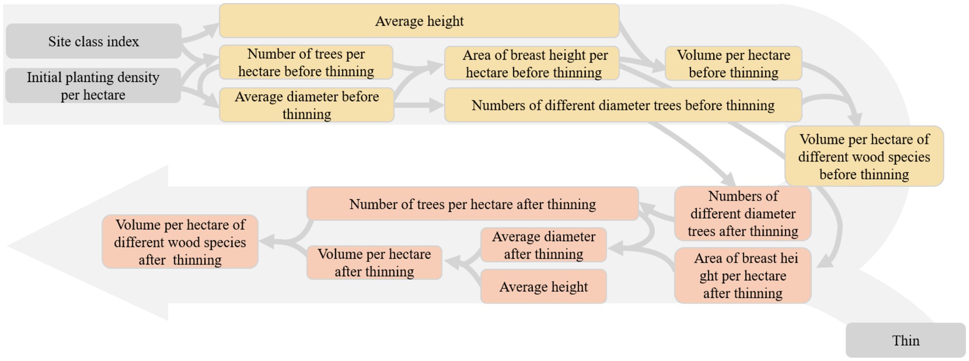
Figure 1. Forest simulation process of stands with thinning.

2.2 Carbon balance calculation

Affected by the discount rate, carbon sequestration income is discounted based on the forestland’s annual net carbon balance. Therefore, we calculate the carbon balance of the forest stand by year, which is the difference between the current year’s net carbon stock and the previous year’s net carbon stock. The net carbon stock is calculated by subtracting the negative carbon release pool from the positive carbon stock pool (Equations 1, 2).

$\begin{array}{ll}{C}_b\left(t\right)=\left(C_p\left(t\right)-C_n\left(t\right)\right)-\left(C_p\left(t-1\right)-C_n\left(t-1\right)\right)& (1)\end{array}$

$\begin{array}{ll}{C}_p\left(t\right)=C_{\mathit{bp}}\left(t\right)+C_{se}\left(t\right)& (2)\end{array}$

where $C_b\left(t\right)$ is the annual carbon balance at Year t (ton C ha⁻¹ yr.⁻¹), $C_p\left(t\right)$ is carbon stock of positive income carbon pool (Pukkala, 2014) at Year t (ton C ha⁻¹), $C_p\left(t-1\right)$ is carbon stock of positive income carbon pool at Year t−1 (ton C ha⁻¹), $C_n\left(t\right)$ is total carbon releases of negative income carbon pool at Year t (ton C ha⁻¹), and $C_n\left(t-1\right)$ is carbon releases of negative income carbon pool at Year t−1 (ton C ha⁻¹), $C_{\mathit{bp}}\left(t\right)$ is carbon stock of biomass pool at Year t (ton C ha⁻¹) and $C_{se}\left(t\right)$ is the substitution effects of wood products.

The biomass carbon pool is calculated through different organ carbon stock models (Dong, 2015; Dong et al., 2019b) for branches, stems, leaves, and roots. In addition, carbon sequestration should also consider the carbon emissions due to substitution effects when commercial products and commercial materials can replace resources, such as steel and fossil fuels. When these substitutes are used, they reduce the production of alternative resources and decrease CO₂ emissions during their production process (Pukkala, 2011; Knauf et al., 2016). When products replace steel or concrete in construction, their production stage usually consumes less fossil energy. For example, the energy consumption of wood processing is significantly lower than that of high-temperature calcination technology in cement production (Hurmekoski et al., 2022). Wood processing facilities often utilize renewable energy from wood residues such as sawdust, further reducing dependence on fossil fuels (Leskinen et al., 2018). The cascading use of wood (repeatedly recycled into low-value products before final disposal) extends its service life and reduces the demand for raw materials (Brunet-Navarro et al., 2021). Different products have varying substitution rates (Knauf et al., 2016). Before the first thinning or harvesting, carbon emissions are primarily from forest litter. After the first thinning or harvesting, carbon emissions include the release of harvest residues, annual litter carbon release, forest product carbon emissions (commercial product carbon emissions and commercial material carbon emissions), and biofuels emissions (assuming that forest owners use 20% of the leaves and branches from harvest residues as biofuels to generate income) (Figure 2; Başkent and Kašpar, 2023). Although the role of biofuels in mitigating climate change has been a subject of debate (Searchinger et al., 2009, 2018; McKechnie et al., 2011), some studies suggest that increased demand for biofuels can also improve forest carbon stocks, and expanding the use of wood-based bioenergy can lead to a net carbon benefit (Favero et al., 2020). Different carbon pool release mechanisms vary, including gradual release and immediate release, with different values of life cycle (t) and decomposition rate (k) (Table 1; Pukkala, 2011, 2014; Dong et al., 2022). The carbon emissions are calculated as follows (Equation 3):

$\begin{array}{ll}{C}_r\left(t\right)=C_r\left(0\right)e^{-kt}& (3)\end{array}$

where $C_r\left(t\right)$ is the dry mass remaining after t years (ton C ha⁻¹); $C_r\left(0\right)$ is the initial dry mass (ton C ha⁻¹); t is the time that has passed (a); and k is an annual decomposition rate.

Figure 2

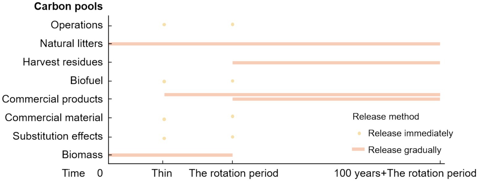
Figure 2. Carbon pool occurrence period.

Table 1

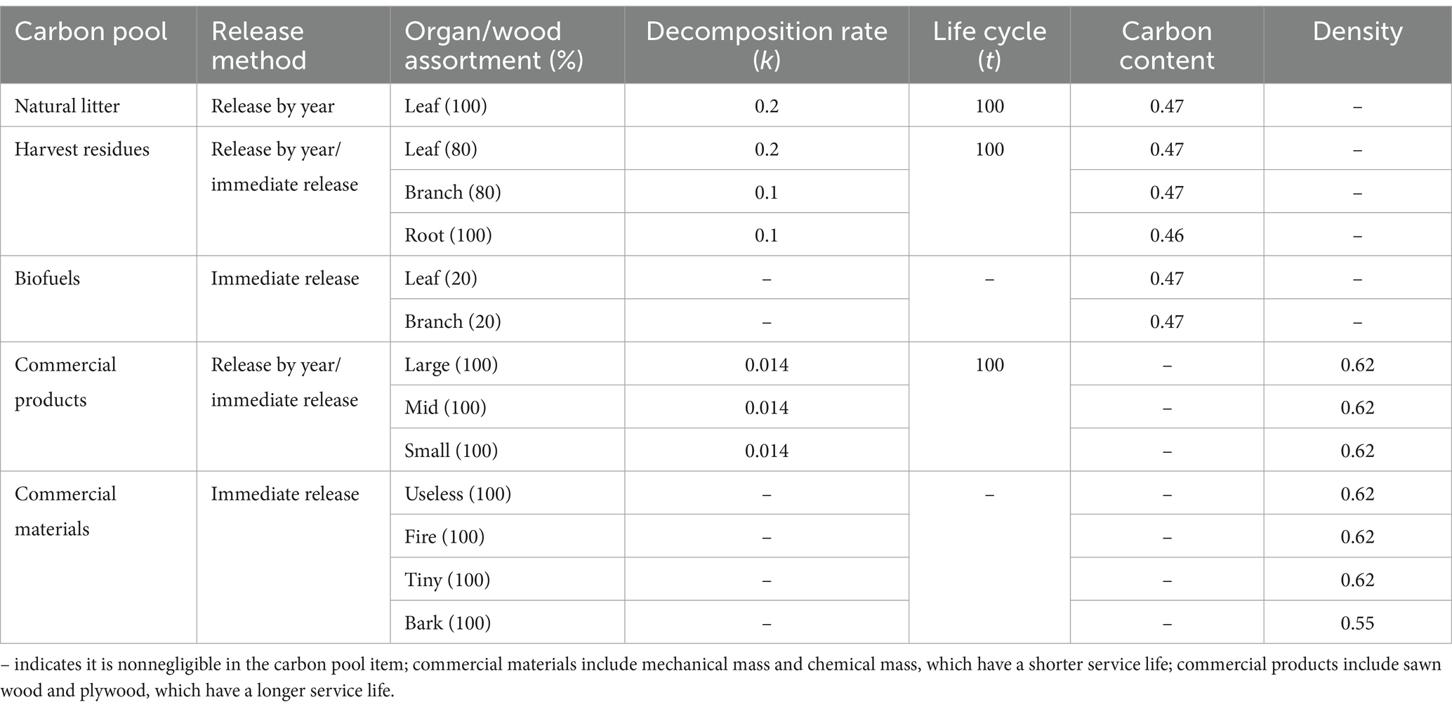
Table 1. The type of release, organ and its proportion of the organ, decomposition rate (k), life cycle $\left(t\right)$, carbon content and density of different carbon release pools.

The CO₂ generated during manufacturing, harvesting, and transportation processes by using fossil fuels should also be considered (Pukkala, 2011; Knauf et al., 2016; Dong et al., 2022). Manufacturing releases were assumed to be a certain proportion of the carbon content of the processed wood (Pukkala, 2014). By combining volume with wood fresh weight density (Lee and Choi, 2016), truckload capacity, and fuel consumption, assuming a total transportation distance of 200 km, carbon emissions during the transportation process are calculated based on fuel consumption. Harvesting emissions were calculated as follows (Equation 4):

$\begin{array}{ll}{R}_h=\frac{3.0-0.05\ast D_g}{100}\ast 100\%& (4)\end{array}$

where $R_h$ is the percentage of harvesting release to total carbon stock (%) and $D_g$ is the average diameter of the stand (cm).

2.3 Scenario analysis

This study simulated eight scenarios to study the impact of different carbon pools on overall forest management measures. Scenario 1 only includes revenues from commercial products, materials, and biofuels. Scenario 2 includes revenue from both commercial and commercial material, biofuel revenue, and revenue from living biomass carbon pools. The remaining six scenarios are built upon Scenario 2 by sequentially adding new carbon pools (Table 2).

Table 2

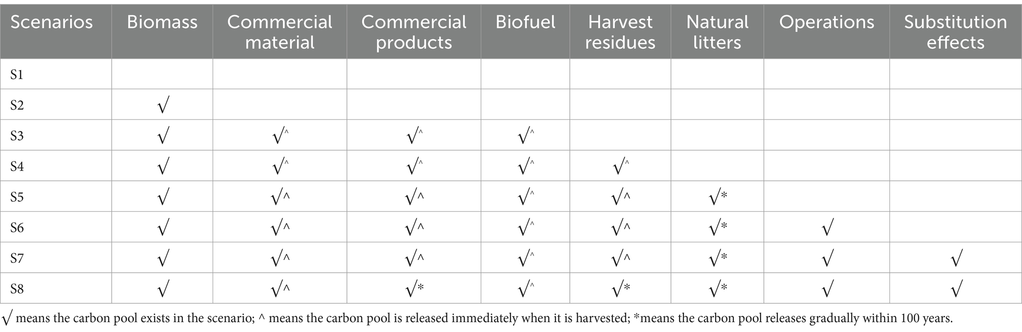
Table 2. The carbon pools considered for S1–S8.

2.4 Forest management model

Based on the Faustmann model, integrated with the Hartman model, and incorporating additional forest management strategies into the forest simulation process based on the rotation period, this study explores stand management measures by combining timber revenue, biofuel revenue, and carbon sequestration revenue as the total stand income (Equation 5) (Creedy and Wurzbacher, 2001; Hoel et al., 2014; Dong et al., 2020). Although the collection of biofuels reduces the carbon storage of harvested residues in forest stands, the positive effects of biofuel on carbon balance would increase through substitution effect if longer periods (more than 30 years) were considered (Pukkala, 2014).

$\begin{array}{ll}NPV\left(t\right)=P_i^w{V}_i\left(t\right)+P^c{C}_b\left(\mathrm{t}\right)+P^f{M}_f\left(t\right)& (5)\end{array}$

where $NPV\left(t\right)$ is the net present value at year t (CNY ha⁻¹); $P_i^w$ is the price of different wood assortments (CNY m⁻³), including commercial products and commercial material (i means different wood assortments; Table 1); $V_i\left(t\right)$ is the volume of different wood assortments at year t (m³ ha⁻¹); $P^c$ is the carbon price (CNY ton⁻¹ C); $P^f$ is the biofuel price (CNY ton⁻¹ or CNY m⁻³); and $M_f\left(t\right)$ is the weight or volume of biofuels at year t (ton or m⁻³). $M_f\left(t\right)$ is calculated through the living biomass of leaves and branches in year t (Equation 6):

$\begin{array}{ll}{M}_f\left(t\right)=0.2\times \left(\frac{C_{\mathit{leaf}}\left(t\right)}{c{t}_{\mathit{leaf}}}+\frac{C_{\mathit{branch}}\left(t\right)}{c{t}_{\mathit{branch}}}\right)& (6)\end{array}$

where $C_{\mathit{leaf}}\left(t\right)$ is the carbon stock of leaves in year t (ton C ha⁻¹); $C_{\mathit{branch}}\left(t\right)$ is the carbon stock of branches in year t (ton C ha⁻¹); $c{t}_{\mathit{leaf}}$ is the carbon content of leaves (ton C ton⁻¹); and $c{t}_{\mathit{branch}}$ is the carbon content of branches (ton C ton⁻¹).

The NPV (S8) is calculated annually from the 10th year to the 100th year for various combinations of N0 (2,500 tree ha⁻¹, 3,333 tree ha⁻¹, 4,444 tree ha⁻¹) and SCI (14 m–20 m), for a total of 21 combinations, with different thinning conditions including thinning frequency (0–3), the first thinning intensity at 20% and subsequent thinning intensity at 10–40%, covering a period from the 10th to 100th year. For all these combinations, the one that maximizes the NPV is selected. At this point, the year corresponds to the optimal rotation period for the stand, and the thinning intensity and frequency represent the optimal thinning strategy.

2.5 Sensitivity analysis

Using an N0 of 3,333 tree ha⁻¹, SCI of 16 m, a carbon price of 100 CNY ton⁻¹ C (Carbon Emissions Trading Network, n.d.), thinning intensity of 10%, and an interest rate of 5% as the baseline scenario, variations in N0, SCI, and carbon price (Table 3) were explored to investigate their impact on stand management strategies and NPV.

Table 3

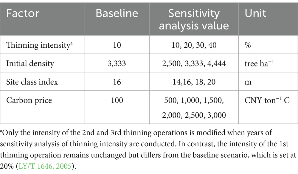
Table 3. Different sensitivity analysis methods.

3 Result

3.1 Development of carbon and volume under the baseline scenario

3.1.1 Effects of thinning on stand volume

The total volume gradually increases over time, rising with a greater frequency of thinning under the baseline scenario, as shown in Figure 3A. Each thinning operation causes a rapid increment in volume. However, the rate of increase slows, and thinning becomes less effective in countering this decline over time. As the thinning frequency increases, the total volume’s growth rate decreases gradually. Without thinning, the volume nears its maximum around the 68th year, reaching 482 m³ ha⁻¹, with an annual growth rate below 2 m³ ha⁻¹ yr.⁻¹. By the end of 100 years, the volume reaches 511 m³ ha⁻¹, with a yearly growth of 0.04 m³ ha⁻¹ yr.⁻¹. Total volumes for thinning frequencies of 1–3 times surpass the unthinned scenario in the 55th year, achieving final volumes of 636 m³ ha⁻¹, 702 m³ ha⁻¹, and 761 m³ ha⁻¹, respectively.

Figure 3

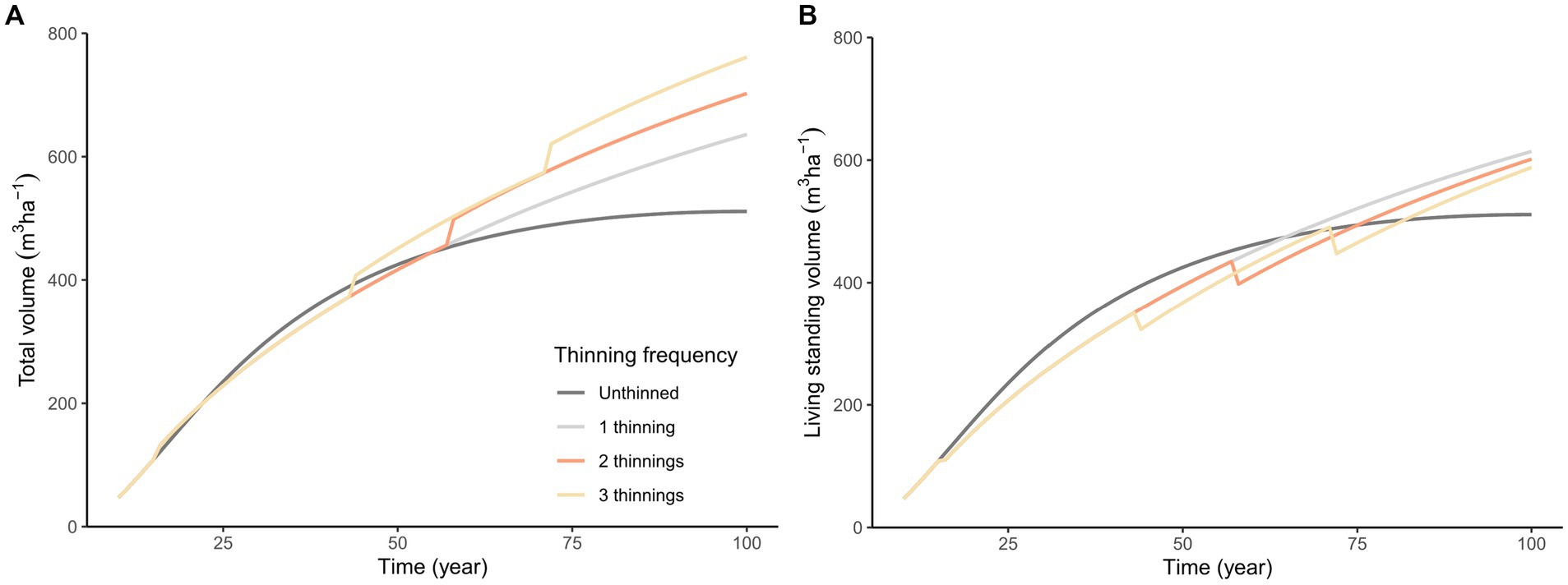
Figure 3. Total volume (A) and living standing volume (B) change over time with thinning under the baseline scenario.

In Figure 3B, the living standing volume gradually increases under the baseline scenario. Each thinning operation, results in a rapid reduction in living standing volume. However, the growth rate in living standing volume improves as the thinning frequency increases. For 1–3 thinnings, living standing volumes (475.62 m³ ha⁻¹ at 65th year, 499 m³ ha⁻¹ at 76th year, and 504 m³ ha⁻¹ at 82nd year) exceed those of the unthinned scenario (475 m³ ha⁻¹, 495 m³ ha⁻¹, 503 m³ ha⁻¹) and maintain higher levels through to the 100th year. By then, living standing volumes for 1–3 thinnings reach 614 m³ ha⁻¹, 602 m³ ha⁻¹, and 588 m³ ha⁻¹, respectively, compared to 511 m³ ha⁻¹ for the unthinned scenario. Volumes with thinning consistently surpass the unthinned scenario, with a single thinning yielding the highest living standing volume.

3.1.2 Effects of thinning on carbon balance

The total carbon stock increases over time under the baseline scenario. By the end of 100 years, as shown in Figure 4A, the total carbon stock with thinning was significantly higher than without thinning. Although there are slight differences based on the frequency of thinning and more frequent thinning results in slightly higher carbon stock, these differences are not substantial. After the first thinning, the total carbon stock reaches 54 ton C ha⁻¹, slightly below the unthinned stock of 55 ton C ha⁻¹, and carbon sequestration also remains lower at this stage (Figure 4B). However, with thinning, the annual rate of decrease in carbon sequestration gradually declines each year, while it continues to rise in the unthinned scenario. Consequently, carbon sequestration with thinning surpasses that without thinning by the 39th year. When thinning occurs 1–3 times, total carbon stock surpasses the unthinned scenario by the 71st year, 68th year, and 66th year, with values reaching 180, 179, and 178 ton C ha⁻¹, respectively, compared to the unthinned values of 180, 178and 177 ton C ha⁻¹.

Figure 4

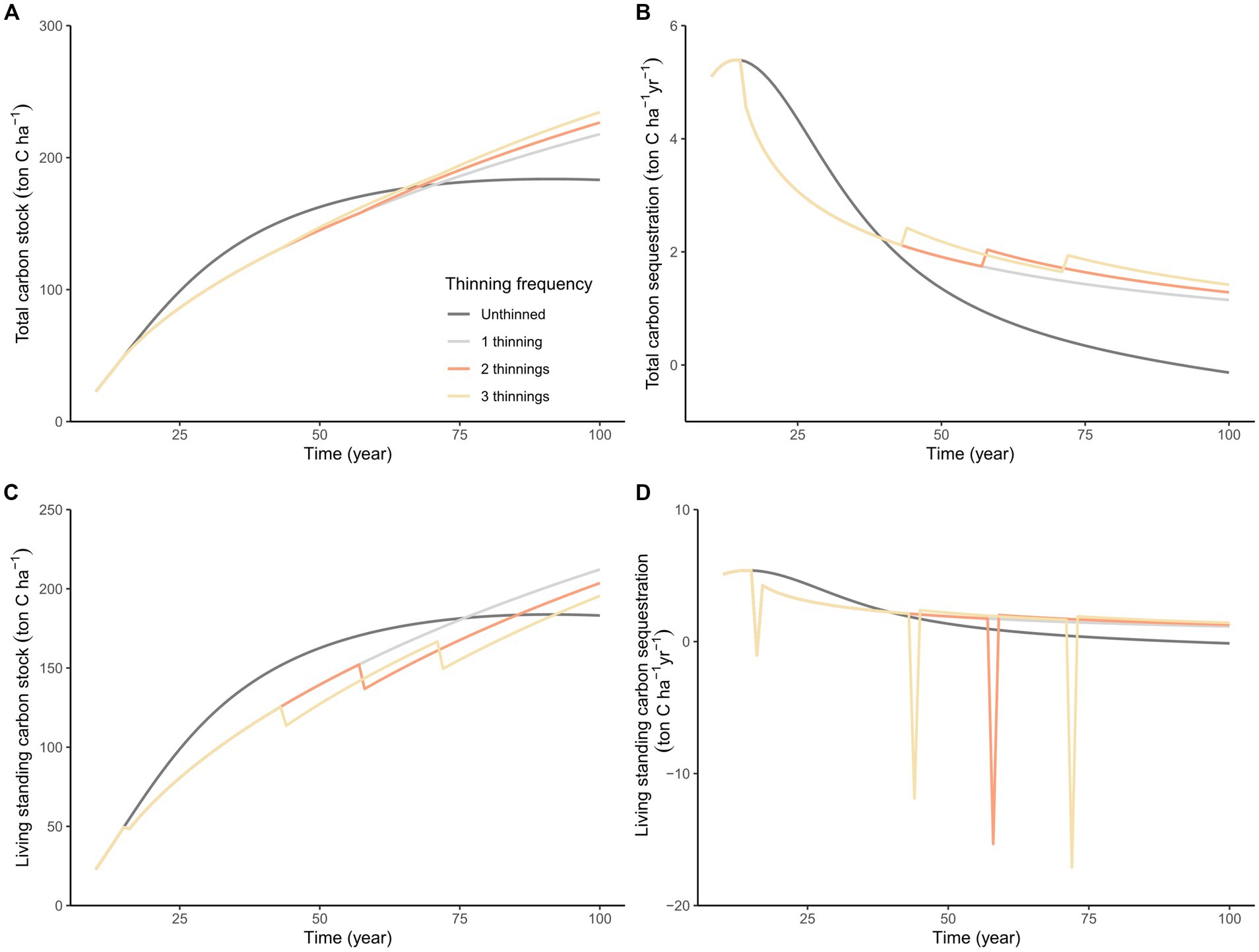
Figure 4. Total carbon stock (A), total carbon sequestration (B), living standing carbon stock (C), and living standing carbon sequestration (D) change over time with thinning under the baseline scenario.

Compared to total carbon stock, thinning frequency has a more pronounced impact on living standing carbon stock under the baseline scenario (Figure 4C). After the first thinning, the living standing carbon stock is noticeably lower than that without thinning. However, with thinning, the rate of decrease in carbon sequestration slows each year, while it continues to rise in the unthinned scenario (Figure 4C). By the 40th year, living standing carbon sequestration with thinning surpassed the unthinned levels (Figure 4D). Following 1–3 thinnings, living standing carbon stock exceeds the unthinned scenario by the 76th, 86th, and 93rd year, with values of 182, 185, and 185 ton C ha⁻¹, respectively, compared to the unthinned values of 182, 184 and 184 ton C ha⁻¹.

The overall trend of the carbon balance gradually increases and then decreases over time under the baseline scenario. However, the rate of decrease slows starting from the 20th year. Between the 10th year and the 100th year, the carbon balance remains positive under all thinning conditions. The carbon balance peaks at 4.03 ton C ha⁻¹ yr.⁻¹ in the 12th year. Before the 56th year, the carbon balances of all thinning treatments were lower than that of the unthinned forest stands. The carbon balances for 1–3 thinnings exceed that of the unthinned forest stands in the 60th year (1.06 ton C ha⁻¹ yr.⁻¹), 58th year (1.10 ton C ha⁻¹ yr.⁻¹), and 57th year (1.12 ton C ha⁻¹ yr.⁻¹). After the 60th year, the carbon balance of all thinning forest stands exceeded that of unthinned stands (1.06 ton C ha⁻¹ yr.⁻¹). By the end of 100 years, the carbon balance for the unthinned, 1 thinning, 2 thinnings, and 3 thinnings are 0.62, 0.62, 0.62, and 0.60 ton C ha⁻¹ yr.⁻¹, respectively (see Figure 5).

Figure 5

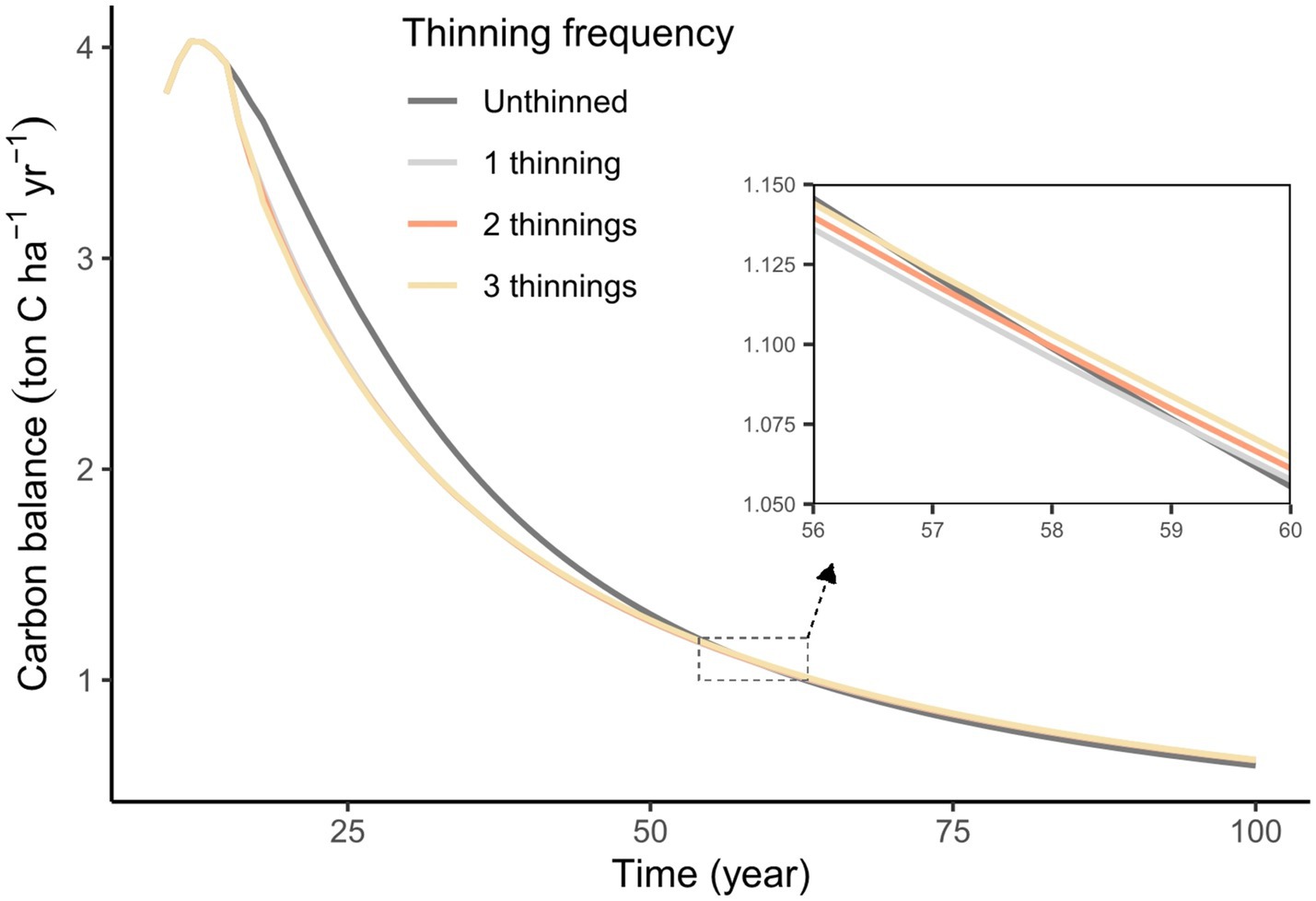
Figure 5. Carbon balance changes over time with different thinning frequencies.

3.2 Carbon sequestration and timber composite operation

3.2.1 Effect of different carbon pools on the optimal rotation

The introduction of thinning significantly influences the optimal rotation period for forest stands when carbon income is considered under the baseline scene. The optimal rotation period is 27 years without thinning, while a single thinning extends it by 15 to 42 years. Furthermore, increasing the thinning frequency will further lengthen the optimal rotation period; as the thinning frequency rises from 1 to 3, the optimal rotation period increases by an additional 5 years. However, thinning reduces the NPV of the total carbon stock, unlike the rotation period. With one thinning, the NPV of the total carbon stock is 6,267 CNY ha⁻¹, which is 664 CNY ha⁻¹ lower than the NPV without thinning. As the thinning frequency increases, the NPV of the total carbon stock gradually rises, but the increment is relatively small. With three thinnings, the NPV of the total carbon stock is 6,320 CNY ha⁻¹, which is 51 CNY ha⁻¹ more than that with one thinning. Thinning reduces the NPV of biomass carbon stock and substitution effects. The increase in thinning frequency leads to decreased commercial products and increased commercial materials, but they have different substitution effects (Knauf et al., 2016). Therefore, as the thinning frequency increases, substitution effects decrease. With one thinning, the NPV of the biomass carbon stock decreases by 466 CNY ha⁻¹, and the substitution effect decreases by 1,485 CNY ha⁻¹. Although thinning increases the NPV of the carbon release pool, with one thinning, the NPV of the carbon release pool is −1,642 CNY ha⁻¹, representing a 1,288 CNY ha⁻¹ increase relative to unthinned, but this increase does not offset the reduction in substitution effects and biomass carbon stock. Increasing thinning frequency results in a reduction in the NPV of substitution effects. The NPV of substitution effects with three thinnings decreases by 263 CNY ha⁻¹ compared to one thinning, which is less than the combined increment in biomass carbon stock (65 CNY ha⁻¹) and NPV of carbon release (249 CNY ha⁻¹) (see Table 4).

Table 4

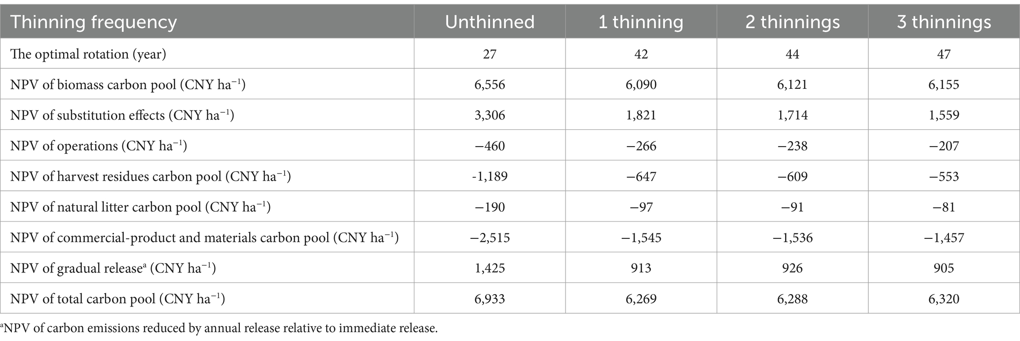
Table 4. The optimal rotation period and the net present value (NPV) of different carbon pools with different thinning frequencies considering the benefits of carbon only.

3.2.2 Composite operation with different carbon pools

Without thinning, carbon pools do not significantly impact the optimal rotation under the baseline scenario. However, when thinning is introduced, increasing the number of carbon pools delays the optimal rotation period by 3 to 6 years. However, including substitution effects and delayed release returns the optimal rotation period to around the same as Scenario 1, weakening or eliminating the influence of carbon pool addition on the optimal rotation period. Except for Scenario 7, the optimal rotation period either increases or remains unchanged with an increase in thinning frequency. In Scenarios 1, 2, and 8, the optimal rotation period is identical for 1 thinning and unthinned, both 27 years. In Scenario 7, the optimal rotation period is most extended for 2 thinnings (30 years), followed by 3 thinnings (29 years), 1 thinning (28 years), and unthinned (27 years).

The addition of carbon sequestration increases the NPV of each scenario while adding a carbon emission decreases the NPV of each scenario. Among all scenarios, NPV with 1 thinning is the lowest, while 3 thinnings has the highest NPV. The NPV of S8 is 22,856 CNY ha⁻¹ for 1 thinning, while for the other thinning conditions: 3 thinnings (28,425 CNY ha⁻¹) > 2 thinnings (25,862 CNY ha⁻¹) > unthinned (23,787 CNY ha⁻¹). The difference in NPV among different scenarios decreases with the increase of thinning frequency, and the sensitivity of NPV to carbon pool decreases with the increase of thinning frequency. The standard deviation of NPV among different scenarios is 2,377 CNY ha⁻¹ when thinning is not carried out, and 2,059 CNY ha⁻¹ when thinning is carried out three times. The increase of thinning frequency reduces it by 318 CNY ha⁻¹. NPV changes of scenarios 3, 4, 5, and 6 are small, with a standard deviation of about 30% relative to the standard deviation of all scenarios. Among them, the standard deviation of NPV for three thinning cycles is only 537 CNY ha⁻¹, which is 26.06% of the standard deviation of all scenarios. The impact of harvesting residue carbon pool, annual litter carbon pool, and operations on NPV is insignificant. With the increase of thinning frequency, the sensitivity of NPV to these three carbon pools decreases more than other carbon pools (see Figure 6).

Figure 6

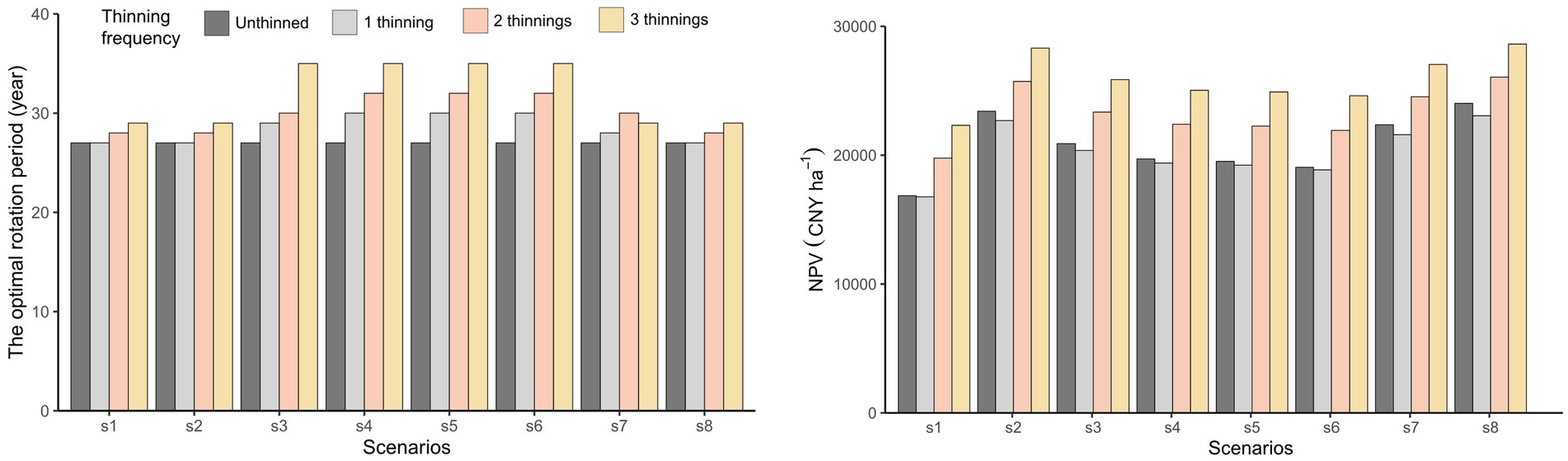
Figure 6. The optimal rotation period and the net present value (NPV) of S1-S8 with different thinning frequencies.

3.2.3 Composite operation under different combinations of site class index and initial planting density

By comparing the NPVs of S8, forest managers can determine the best management strategy based on various combinations of N0 and SCI. In all combinations, thinning occurs three times. When N0 is 2,500 tree ha⁻¹, the optimal rotation period initially increases and then decreases as SCI rises. Surprisingly, the rotation period does not shorten with the improvement of SCI, which is different from other N0. The optimal thinning intensity remains unchanged, but the NPV increases with a higher SCI. When the SCI is 15 m, the thinning intensity is at its lowest (30%), and the optimal rotation period is 26 years, resulting in an NPV of 23,217 CNY ha⁻¹. When the SCI is 17 m, the optimal rotation period reaches its maximum of 29 years, and the optimal thinning plan involves 3 thinnings, with 40% intensity for the second and third thinnings, resulting in an NPV of 36,521 CNY ha⁻¹. When the SCI is 20 m, the NPV peaks at 49,681 CNY ha⁻¹, and the optimal management plan is a rotation period of 23 years with 3 thinnings, where the first thinning is at 20% intensity, and both the second and third thinning are at 40% intensity.

When N0 is 3,333 tree ha⁻¹, the optimal rotation period increases as SCI rises. The optimal thinning intensity initially decreases and then increases with higher SCI, and the NPV increases with higher SCI. The optimal rotation period for SCI between 14 m and 16 m remains the same as for N0 of 2,500 tree ha⁻¹ at 26 years. For instance, at an SCI of 14 m, the optimal thinning plan involves 3 thinnings: the first at 20% intensity and the second and third thinning at 40% intensity, resulting in an NPV of 27,215 CNY ha⁻¹. For SCI values between 15 m and 17 m, the optimal thinning intensity is lowest at 30%. At an SCI of 17 m, the optimal management plan includes a 23-year rotation period with 3 thinnings, where the first thinning is at 20% intensity, and the second and third thinnings are at 30% intensity, resulting in an NPV of 41,749 CNY ha⁻¹. When SCI reaches 20 m, the NPV peaks at 61,108 CNY ha⁻¹, with the optimal management plan being 3 thinnings: the first thinning at 20% intensity, and the second and third thinning at 40% intensity, with a rotation period of 20 years.

When N0 is 4,444 tree ha⁻¹, the optimal rotation period increases as SCI rises. The optimal thinning intensity initially decreases and then increases with a higher SCI, and the NPV also increases with a higher SCI. For SCI values between 17 m and 20 m, the optimal rotation period is the same as for N0 of 3,333 tree ha⁻¹. At an SCI of 20 m, the optimal management plan includes 3 thinnings: the first thinning at 20% intensity, and the second and third thinning at 40% intensity, with a rotation period of 20 years. This results in the maximum NPV of 81,388 CNY ha⁻¹. When the SCI is 17 m, the optimal thinning intensity is minimized at 30%, and the optimal management plan involves 3 thinnings: the first thinning at 20% intensity, and the second and third thinning at 30% intensity, with a 23-year rotation period, resulting in an NPV of 54,372 CNY ha⁻¹. When the SCI is 14 m, the NPV is minimized at 36,369 CNY ha⁻¹, with an optimal management plan of 3 thinnings: the first thinning at 20% intensity, and the second and third thinning at 40% intensity, with a 26-year rotation period (see Table 5).

Table 5

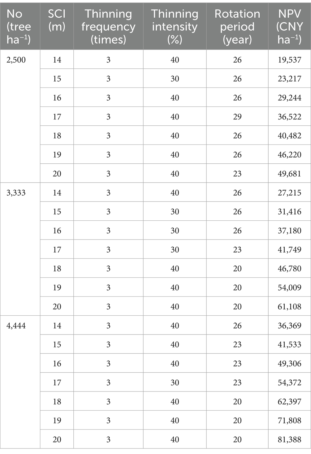
Table 5. The optimal management strategy with different combinations of initial planting density and site class index.

3.3 Sensitivity analysis

3.3.1 Sensitivity of thinning intensities

As thinning intensity increases, the optimal rotation period is delayed. For unthinned and a single thinning, the optimal rotation periods remain unchanged at 27 years and 28 years, respectively, because the thinning intensity only changes during the second and third thinnings. With two thinnings, the optimal rotation period gradually increases with higher thinning intensity. When the thinning intensity reaches 30%, the optimal rotation period reaches 32 years, but it decreases to 28 years at 40% intensity. With 3 thinnings, the optimal rotation period is delayed to 35 years at 30% thinning intensity and remains the same.

In all cases, the NPV increases with higher thinning intensities and frequency. Because the thinning intensity only changes during the second and third thinning, the NPV of the forest without thinning and the NPV of the forest after thinning remain unchanged, at 24,018 CNY ha⁻¹ and 25,878 CNY ha⁻¹ for each thinning intensity. For 2 thinnings, the maximum NPV is 33,692 CNY ha⁻¹ at 40%, while the minimum is 28,446 CNY ha⁻¹ at 10%. For 3 thinnings, the maximum NPV is 41,738 CNY ha⁻¹ at 40%, while the minimum is 31,285 CNY ha⁻¹ at 10%. The NPV demonstrates greater sensitivity to thinning frequency as thinning intensity increases. When the thinning frequency increases from two to three, the NPV rises by 8,046 CNY ha⁻¹, representing a 23.89% increase at a 40% thinning intensity. At a thinning intensity of 30%, the increase is 6,035 CNY ha⁻¹ or 18.68%. Similarly, at 20% intensity, the NPV increases by 4,815 CNY ha⁻¹, corresponding to a 15.81% rise, while at 10% intensity, the increase is 2,839 CNY ha⁻¹, reflecting a 9.98% change (see Figure 7).

Figure 7

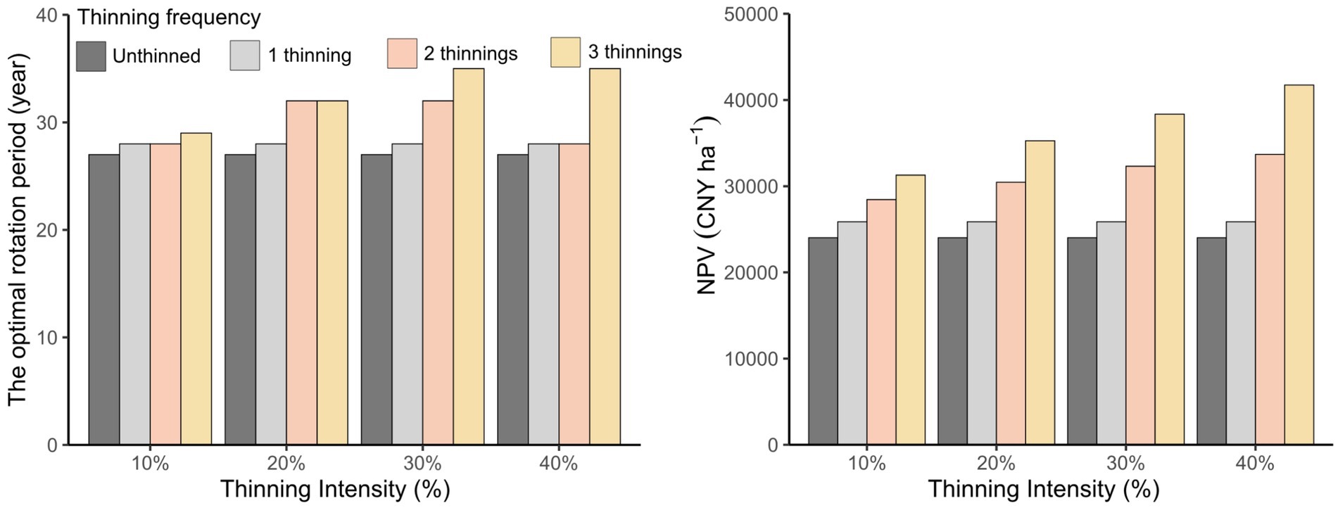
Figure 7. The optimal rotation period and net present value (NPV) with different thinning methods.

3.3.2 Sensitivity of initial planting densities

The optimal rotation period decreases as N0 increases. When N0 is 2,500 tree ha⁻¹, the optimal rotation period increases with thinning frequency, reaching 27, 29, 30, and 32 years, respectively. The optimal rotation period for N0 of 3,333 tree ha⁻¹ is 3–4 years longer than for N0 of 3,333 tree ha⁻¹. For N0 of 3,333 and 4,444 tree ha⁻¹, the longest optimal rotation periods are 29 and 26 years, respectively, with 3 thinnings. The NPV increases as N0 rises. For N0 of 2,500 tree ha⁻¹, the NPV increases with rising thinning frequency, reaching 17,653 CNY ha⁻¹, 17,758 CNY ha⁻¹, 19,938 CNY ha⁻¹, and 22,176 CNY ha⁻¹ for 0, 1, 2, and 3 thinnings, respectively. However, for N0 of 3,333 and 4,444 tree ha⁻¹, the NPVs of unthinned are 958 CNY ha⁻¹ and 976 CNY ha⁻¹ higher than for 1 thinning (see Figure 8).

Figure 8

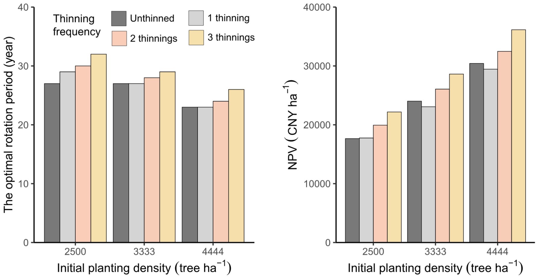
Figure 8. The optimal rotation period and net present value (NPV) with different thinning frequencies in three levels of initial planting density.

3.3.3 Sensitivity of site class indexes

The optimal rotation period decreases as SCI increases, and the effect of thinning frequency on the optimal rotation period varies with SCI. When SCI is 14 m, the optimal rotation period, from highest to lowest, is 33 years (2 thinnings), 32 years (3 thinnings), 29 years (unthinned), and 28 years (1 thinning). However, when SCI exceeds 14 m, the optimal rotation period increases with more thinning. At an SCI of 16 m, the longest optimal rotation period is 29 years with 3 thinnings.

The NPV increases as SCI rises. For 3 thinnings, the maximum NPV occurs at an SCI of 20 m, reaching 49,490 CNY ha⁻¹. This is 2.44, 1.73, and 1.29 times NPV at SCI of 14 m, 16 m, and 18 m, respectively. As SCI increases, the NPV from 1 thinning also increases, surpassing the NPV from unthinned at an SCI of 18 m. At this SCI, the NPV from 1 thinning is 31,298 CNY ha⁻¹, which is 49 CNY ha-1 higher than for unthinned. As SCI increases, the sensitivity of the NPV to thinning also gradually increases. For all SCI values, the increase in NPV compared to 1 thinning, from highest to lowest, is as follows: 8,541 CNY ha⁻¹ (20 m), 7,179 CNY ha⁻¹ (18 m), 5,563 CNY ha⁻¹ (16 m), and 4,281 CNY ha⁻¹ (14 m) (see Figure 9).

Figure 9

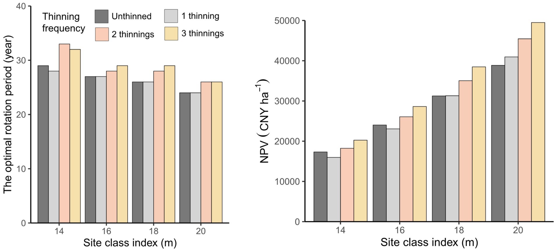
Figure 9. The optimal rotation period and net present value (NPV) with different thinning frequencies in four levels of site class index.

3.3.4 Sensitivity of carbon prices

The optimal rotation period is delayed as carbon prices and thinning frequency increase. Without thinning, the optimal rotation period remains unchanged. With 1 thinning, the minimum carbon price required to delay the optimal rotation period by 1 year is 1,500 CNY ton⁻¹ C, resulting in an optimal rotation period of 29 years. When 2 thinnings, the optimal rotation period remains 30 years. For 3 thinnings, as the carbon price increases from 500 to 1,000 CNY ton⁻¹ C, the optimal rotation period extends from 29 to 32 years, a delay of 3 years.

The NPV increases with higher carbon prices. At different carbon prices, the trend in the NPV remains consistent. Taking a carbon price of 3,000 CNY ton⁻¹ C as an example, the NPVs from highest to lowest are as follows: unthinned, 3 thinnings, 2 thinnings, and 1 thinning. As carbon prices rise, the sensitivity of the NPV to thinning frequency increases. Comparing the unthinned stands with the thinned forest stands, it can be observed that the difference in NPV has increased from 4,668 CNY ha⁻¹ at a carbon price of 500 CNY ton⁻¹ C to 27,669 CNY ha⁻¹ at a carbon price of 3,000 CNY ton⁻¹ C (see Figure 10).

Figure 10

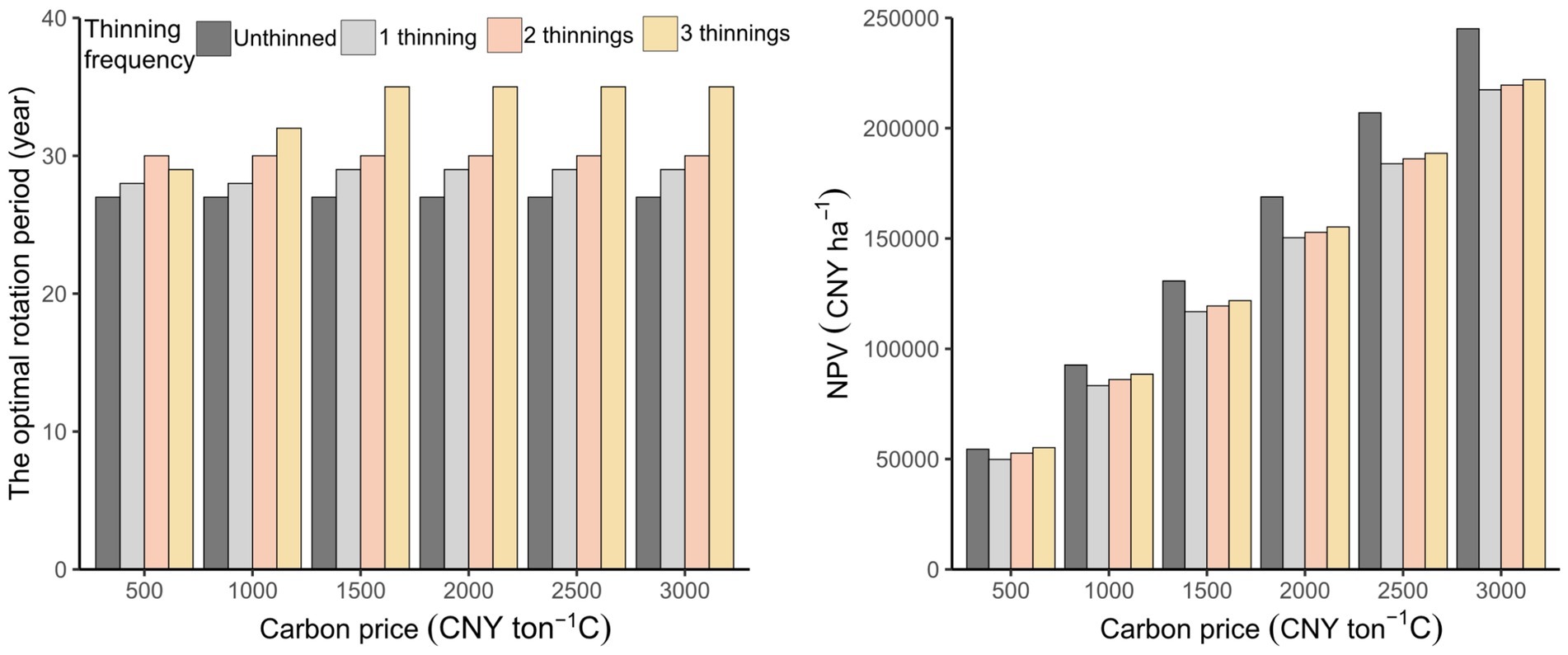
Figure 10. The optimal rotation period and the net present value (NPV) with different thinning frequencies for six different carbon prices.

3.3.5 Sensitivity of interest rates

The optimal rotation age of a forest stand decreases as the interest rate increases. Taking the scenario of three thinnings as an example, the optimal rotation age is 68 years when the interest rate is 1%, but it decreases to 22 years when the interest rate rises to 9%. The impact of thinning frequency on the optimal rotation age varies under different interest rates. At a 1% interest rate, a higher thinning frequency leads to a longer optimal rotation age, with the shortest rotation age of 60 years observed for stands without thinning. However, at a 3% interest rate, stands with 1 thinning have an optimal rotation age of 36 years, 2 years longer than those with 2 thinnings. As the interest rate increases, the reduction rate in the optimal rotation age diminishes. For instance, with three thinnings, an increase in the interest rate from 1 to 3% shortens the rotation age from 68 to 38 years (a reduction of 30 years). However, when the interest rate rises from 7 to 9%, the rotation age decreases from 23 to 22 years, representing only a one-year reduction.

The NPV of the forest stand decreases with increasing interest rates. For stands thinned three times, the NPV drops from 369,052 CNY ha⁻¹ at a 1% interest rate to 5,718 CNY ha⁻¹ at a 9% interest rate, marking a reduction of 363,334 CNY ha⁻¹. At interest rates of 1, 3, and 9%, the NPV increases with the number of thinnings, with stands without thinning showing the lowest NPVs of 242,739 CNY ha⁻¹, 59,906 CNY ha⁻¹, and 4,079 CNY ha⁻¹, respectively. In contrast, at 5 and 7% interest rates, stands with 1 thinning have the lowest NPV, with values of 23,060 CNY ha⁻¹ and 10,268 CNY ha⁻¹, respectively. As the interest rate increases, the rate of NPV reduction also slows. For example, in stands thinned three times, an increase in the interest rate from 1 to 3% reduces the NPV by 295,010 CNY ha⁻¹ (a 79.94% decrease). However, when the interest rate rises from 7 to 9%, the NPV decreases by only 7,381DB23/T 870CNY ha⁻¹ (a 56.35% decrease) (see Figure 11).

Figure 11

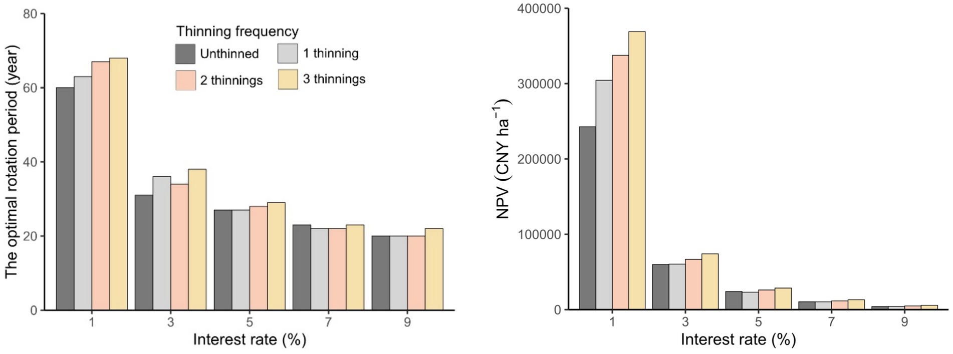
Figure 11. The optimal rotation period and the net present value (NPV) with different thinning frequencies for five different interest rates.

4 Discussion

Due to the difficulty of finding forest stands with SCI and N0 exactly matching and with varying levels of harvesting from 0–3 times and 10–40% complete coverage, and given that process models involve numerous parameters that are difficult to measure (Xue, 2022), the growth and harvest model of forest stands is widely used and widely applied in production practice (Zhang, 2012). This study simulates stand growth using forest yield tables of Heilongjiang Province (DB23/T 1377, 2010). It explores the optimal forest management measures, enabling more accessible extension to different tree species and regions and facilitating the expansion of other tree species and regions. Similar to Dong et al. (2022), this research considers eight carbon pools, including substitution effects and operations, comprehensively modeling forest carbon dynamics. This study further expands the scope of forest management strategies, providing optimal forest management plans for all 21 combinations of different SCIs and N0. Since this study is based on the generalized Faustmann framework, assuming an infinite rotation period, the initial carbon pool does not impact the optimal rotation period for forests (Holtsmark et al., 2013). Holtsmark only considered the impact of the initial carbon pool on the optimal rotation period; however, a large initial stock of dead organic matter draws in the direction of earlier harvest, and therefore, the initial carbon pool has no influence on forest management plans and is disregarded.

The impact of SCI and N0 on stands subject to selective harvesting is consistent with previous research (Dong et al., 2022). However, the influence of carbon prices on stands differs from earlier studies. When the SCI is approximately 14 m, and N0 is 3,333 tree ha⁻¹, a carbon price of 420 CNY ton⁻¹ C will change the optimal rotation period for stands without selective harvesting. When SCI is approximately 18 m, and N0 is approximately 2,500 tree ha⁻¹, a carbon price of 1,000 CNY ton⁻¹ C will increase the optimal rotation period for stands. In contrast, this study found that even with a carbon price of 3,000 CNY ton⁻¹ C, the optimal rotation period for stands without thinning cannot be changed. Only when thinning is applied to stands does the optimal rotation period become postponed with increasing carbon prices. This difference may be related to variations in the combinations of N0 and SCI. For NPV, when the carbon price reaches or exceeds 1,000 CNY ha⁻¹, stands without thinning achieve a higher value. This is likely because unthinned stands maintain a higher living stand carbon stock by the end of the rotation period, thereby prolonging the time of delayed carbon sequestration release. The higher the SCI, the higher the NPV of the forest stand, which is consistent with general research. This study found that the NPV of thinned forest stands is more sensitive to the increase in SCI. When the SCI is 18 m, the NPV of 1 thinning begins to exceed that of unthinned. When the N0 is low, the NPV of 1 thinning is higher than that of unthinned forest stands. When the N0 is high, the NPV of 1 thinning is the lowest. This is because at lower N0, the rotation period of 1 thinning is more extended than that of unthinned forest stands. In this study, when examining the impact of carbon prices on stands, the values for N0 and SCI were 16 m and 3,333 tree ha⁻¹, respectively. Further research is needed to quantitatively analyze how stands with different combinations of SCI and N0 respond to changes in carbon prices. Different researchers have reached different conclusions regarding the impact of thinning on forest stands. Some studies are consistent with the results of this article and show that thinning will improve tree health, wood yield, carbon sequestration capacity (Chen and Chang, 2014), the global aboveground biomass carbon storage of trees, understory vegetation carbon storage, and soil organic carbon storage, but significantly reduced litter carbon storage. And underground biomass carbon storage remains unchanged under thinning (Zhang, 2012); others believe that thinning will weaken the carbon sequestration capacity of forest stands (Sacchelli and Bernetti, 2019). They believe that thinning will increase the carbon stock of trees, and the greater the intensity of thinning, the more significant the increase in carbon stock. However, due to the decrease in the density of forest stands, the stand carbon stock decreases with increasing thinning intensity (Lin et al., 2018). The conflict may be attributed to different thinning plans to achieve different management goals (Zou et al., 2023). The second reason is that they only considered the carbon stock in the stem of the forest stand and ignored the carbon stock in other organs, such as branches, leaves, and roots. The most important reason is that they only considered the living biomass carbon pool in the forest stand, while trees cut by thinning were ignored. Although trees have been thinned, the carbon sequestration capacity of forests should include the thinned trees, and the thinning timber can still be utilized to produce substitution effects. NPV increases with the increase of thinning intensity until it reaches 35% thinning intensity and then decreases with the increase of thinning intensity. The optimal thinning frequency is 2 thinnings (Huang, 2008). In addition, studies have found that in low, medium, and high gradient thinning, moderate to low-intensity thinning recovers more quickly after thinning and makes the forest structure more complex (Liang et al., 2023), which can promote the growth of forest volume (Shen et al., 2019). High thinning can make the forest size structure more uniform and obtain timber forests faster (Liang et al., 2023), but at the same time, high thinning can also cause the forest to transform from a carbon sequestration forest to a carbon source forest, resulting in more excellent carbon release. The production of timber and carbon decreased with increasing intensity and shortening frequency of thinnings, while the provision of mushrooms and blue water generally increased under those conditions (Simon and Ameztegui, 2023).

The substitution effects in this study are all marginal substitution effects, similar to most studies on forest carbon sequestration (Hurmekoski et al., 2022). This is because marginal substitution effects are more suitable for evaluating and comparing the carbon reduction potential in different wood use scenarios, while absolute substitution effects are rarely studied separately and are usually used as a result indicator in comprehensive carbon assessments (Leskinen et al., 2018). This research has found that thinning three times at 40% intensity and a rotation period of 35 years is the optimal forest management measure. This thinning intensity is much higher than the LY/T 1646 (2005). This finding is consistent with the results of Pukkala (2014). Since carbon sequestrations accumulate fastest in middle-aged and young forests, Sacchelli and Bernetti (2019) found that shorter rotation periods benefit carbon stocks, while thinning can reduce or even restore the decrease in the forest carbon sequestration rate. Chen and Chang (2014) compared the growth rate of the 11–20 age class after different thinning intensities in each period. They found that the growth rate of the forest stand was the largest when the thinning intensity was 40% in the first thinning time, and in the subsequent 2nd to 4th thinning, when the thinning intensity was 60%, the stand growth rate was at a maximum. Buchholz et al. (2021) find that forest management optimized for maximal financial return, which rewards short-term net cash flow through discounting, incentivizes mid-rotation thinnings, which provide both early cash flow from selling pulpwood or pellet feedstock, as well as a limited amount of small diameter sawlogs where removed trees already meet sawlog dimensions. According to LY/T 1646 (2005), this study simulated the growth of a forest stand with a maximum of three thinnings. However, some researchers found that five is the optimal thinning frequency for pine trees (Cao et al., 2010), so this study found that whether the thinning frequency reached three times was caused by scenario setting restrictions. In this study, the optimal rotation period for different conditions was around 30 years. This is because the rotation period for larch plantations varies with alternative management objectives. Compared to the maturity age, the economic maturity age is relatively small. According to Li et al. (1994), when the interest rate is 6% and the SCI is 15, the rotation is around 27. As the SCI improves, the rotation period will continue to shorten. In addition, this study only considered the thinning method of lower layer tending, and uniform thinning and upper layer tending are also common thinning methods. Some studies have found that CTR (crop tree release) benefits individual trees’ growth more than traditional thinning methods (Zou et al., 2023). Therefore, subsequent research needs to use goal programming or heuristic algorithms to determine the optimal business plan under unrestricted conditions (Chen and Chang, 2014).

5 Conclusion

In this paper, a theoretical framework based on the Faustmann model to maximize NPV is established and used to determine the optimal forest management plan. This study finds that the carbon balance gradually increases and then decreases over time under the baseline scenario. However, the optimal harvest rotation period is delayed with an increase in thinning frequency and thinning intensity. And the NPV increases with an increase in both thinning frequency and thinning intensity. The sensitivity of NPV to thinning frequency is enhanced with an increase in thinning intensity, SCI, and carbon price. Since this study employs stand yield tables and diameter distribution models to simulate forest growth, it obtains optimal forest management plans for different combinations of N0 and SCI. Taking the baseline scenario (N0 of 3,333 tree ha⁻¹, SCI of 16 m, discount rate of 5%, and carbon price of 100 CNY ton⁻¹) as an example, the optimal forest management plan consists of three thinnings, with the first thinning intensity at 20%, the second and third thinning at 30%, and the harvest rotation period of 26 years. The NPV at this point is 37,180 CNY ha⁻¹.

Data availability statement

The original contributions presented in the study are included in the article/supplementary material, further inquiries can be directed to the corresponding author.

Author contributions

XL: Writing – original draft, Writing – review & editing. WL: Writing – review & editing. LD: Writing – review & editing.

Funding

The author(s) declare that financial support was received for the research, authorship, and/or publication of this article. This research was supported by the National Natural Science Foundation (Grant number 32171778), and the Fundamental Research Funds for the Central Universities (Grant number 2572023AW05).

Acknowledgments

The authors thank Dongyuan Tian and Ying Chen for significant input to the statistical analysis.

Conflict of interest

The authors declare that the research was conducted without any commercial or financial relationships that could be construed as a potential conflict of interest.

Publisher’s note

All claims expressed in this article are solely those of the authors and do not necessarily represent those of their affiliated organizations, or those of the publisher, the editors and the reviewers. Any product that may be evaluated in this article, or claim that may be made by its manufacturer, is not guaranteed or endorsed by the publisher.

References

Asante, P., and Armstrong, G. W. (2012). Optimal forest harvest age considering carbon sequestration in multiple carbon pools: a comparative statics analysis. J. For. Econ. 18, 145–156. doi: 10.1016/j.jfe.2011.12.002

PubMed Abstract | Crossref Full Text | Google Scholar

Asante, P., Armstrong, G. W., and Adamowicz, W. L. (2011). Carbon sequestration and the optimal forest harvest decision: a dynamic programming approach considering biomass and dead organic matter. J. For. Econ. 17, 3–17. doi: 10.1016/j.jfe.2010.07.001

PubMed Abstract | Crossref Full Text | Google Scholar

Başkent, E. Z., and Kašpar, J. (2023). Exploring the effects of various rotation lengths on the ecosystem services within a multiple-use management framework. For. Ecol. Manag. 538:120974. doi: 10.1016/j.foreco.2023.120974

Crossref Full Text | Google Scholar

Brunet-Navarro, P., Jochheim, H., Cardellini, G., Richter, K., and Muys, B. (2021). Climate mitigation by energy and material substitution of wood products has an expiry date. J. Clean. Prod. 303:127026. doi: 10.1016/j.jclepro.2021.127026

Crossref Full Text | Google Scholar

Buchholz, T., Gunn, J. S., and Sharma, B. (2021). When Biomass Electricity Demand Prompts Thinnings in Southern US Pine Plantations: A Forest Sector Greenhouse Gas Emissions Case Study. Front. For. Glob. Change. 4:642569. doi: 10.3389/ffgc.2021.642569

Crossref Full Text | Google Scholar

Cao, T., Valsta, L., and Mäkelä, A. (2010). A comparison of carbon assessment methods for optimizing timber production and carbon sequestration in scots pine stands. For. Ecol. Manag. 260, 1726–1734. doi: 10.1016/j.foreco.2010.07.053

Crossref Full Text | Google Scholar

Carbon Emissions Trading Network (n.d.) Available at: http://www.tanpaifang.com/ (accessed November 27, 2004).

Google Scholar

Chen, Y.-T., and Chang, C.-T. (2014). Multi-coefficient goal programming in thinning schedules to increase carbon sequestration and improve forest structure. Ann. For. Sci. 71, 907–915. doi: 10.1007/s13595-014-0387-z

Crossref Full Text | Google Scholar

Creedy, J., and Wurzbacher, A. D. (2001). The economic value of a forested catchment with timber, water and carbon sequestration benefits. Ecol. Econ. 38, 71–83. doi: 10.1016/S0921-8009(01)00148-3

Crossref Full Text | Google Scholar

DB23/T 1377 (2010). Yield table of main forest types in Heilongjiang Province. Quality and Technical Supervision Bureau of Heilongjiang, Harbin.

Google Scholar

DB23/T 870 (2004). Yield rate table for major tree species in county-level forested areas, 2004. Quality and Technical Supervision Bureau of Heilongjiang, Harbin.

Google Scholar

Dong, L. (2015). Developing individual and stand-level biomass equations in Northeast China forest area. Harbin: Northeast Forestry University.

Google Scholar

Dong, L., Bettinger, P., Qin, H., and Liu, Z. (2022). Optimizing rotation lengths for maximizing carbon balance of larch plantations in Northeast China. J. Clean. Prod. 343:131025. doi: 10.1016/j.jclepro.2022.131025

Crossref Full Text | Google Scholar

Dong, L., Jin, X., Pukkala, T., Li, F., and Liu, Z. (2019a). How to manage mixed secondary forest in a sustainable way? Eur. J. For. Res. 138, 789–801. doi: 10.1007/s10342-019-01196-0

Crossref Full Text | Google Scholar

Dong, L., Liu, Y., Zhang, L., Xie, L., and Li, F. (2019b). Variation in carbon concentration and allometric equations for estimating tree carbon contents of 10 broadleaf species in natural forests in Northeast China. Forests 10:928. doi: 10.3390/f10100928

Crossref Full Text | Google Scholar

Dong, L., Lu, W., and Liu, Z. (2020). Determining the optimal rotations of larch plantations when multiple carbon pools and wood products are valued. For. Ecol. Manag. 474:118356. doi: 10.1016/j.foreco.2020.118356

Crossref Full Text | Google Scholar

Favero, A., Daigneault, A., and Sohngen, B. (2020). Forests: carbon sequestration, biomass energy, or both? Science (New York, NY: Online) 6:eaay6792. doi: 10.1126/sciadv.aay6792

PubMed Abstract | Crossref Full Text | Google Scholar

Gong, Z., O’Hara, K. L., Li, W., and Gu, L. (2019). Optimal forest rotation periods: integrating timber production and carbon sequestration benefits in Pinus tabulaeformis plantations on the Loess Plateau, P.R. China. J. Sustain. For. 38, 591–613. doi: 10.1080/10549811.2019.1598442

Crossref Full Text | Google Scholar

Goodarzi, M. (2017). Climate change for forest policy makers (FAO bulletin translated into Persian).

Google Scholar

Hoel, M., Holtsmark, B., and Holtsmark, K. (2014). Faustmann and the climate. J. For. Econ. 20, 192–210. doi: 10.1016/j.jfe.2014.04.003

PubMed Abstract | Crossref Full Text | Google Scholar

Holtsmark, B., Hoel, M., and Holtsmark, K. (2013). Optimal harvest age considering multiple carbon pools – a comment. J. For. Econ. 19, 87–95. doi: 10.1016/j.jfe.2012.09.002

PubMed Abstract | Crossref Full Text | Google Scholar

Huang, J. (2008). An empirical analysis of adaptability to climate change and risk in forest management (Ph.D.). ProQuest Diss. Theses. North Carolina State University, United States -- North Carolina.

Google Scholar

Hurmekoski, E., Suuronen, J., Ahlvik, L., Kunttu, J., and Myllyviita, T. (2022). Substitution impacts of wood-based textile fibers: influence of market assumptions. J. Ind. Ecol. 26, 1564–1577. doi: 10.1111/jiec.13297

Crossref Full Text | Google Scholar

IPCC (2023). IPCC sixth assessment report (AR6). Available at: https://www.ipcc.ch/report/ar6/syr/

Google Scholar

Knauf, M., Joosten, R., and Frühwald, A. (2016). Assessing fossil fuel substitution through wood use based on long-term simulations. Carbon Manag. 7, 67–77. doi: 10.1080/17583004.2016.1166427

Crossref Full Text | Google Scholar

Koirala, U., Adams, D. C., Susaeta, A., and Akande, E. (2022). Value of a flexible forest harvest decision with short period forest carbon offsets: application of a binomial option model. Forests 13:1785. doi: 10.3390/f13111785

Crossref Full Text | Google Scholar

Lee, D., and Choi, J. (2016). Estimating wood weight change on air drying times for three coniferous species of South Korea. J. For. Environ. Sci. 32, 262–269. doi: 10.7747/JFES.2016.32.3.262

Crossref Full Text | Google Scholar

Leskinen, P., Cardellini, G., González-García, S., Hurmekoski, E., Sathre, R., Seppälä, J., et al. (2018). Substitution effects of wood-based products in climate change mitigation. From Science to Policy. European Forest Institute. doi: 10.36333/fs07

Crossref Full Text | Google Scholar

Li, S., Li, S., and Huang, M. (2017). Effects of thinning intensity on carbon stocks and changes in larch forests in China northeast forest region. J. Resour. Ecol. 8, 538–544. doi: 10.5814/j.issn.1674-764x.2017.05.011

Crossref Full Text | Google Scholar

Li, M., Li, C., Li, C., and Zhang, Y. (1994). Research on the rotation period of Larix olgensis plantations. For. Eng. 1–6. doi: 10.16270/j.cnki.slgc.1994.04.001

Crossref Full Text | Google Scholar

Li, M., Zhong, C., and Li, Y. (1998). A study on the diameter distribution model of Larix gmelinii plantation. J. Nanjing For. Univ. 22, 57–60.

Google Scholar

Liang, R., Xie, Y., Sun, Y., Wang, B., and Ding, Z. (2023). Temporal changes in size inequality and stand growth partitioning between tree sizes under various thinning intensities in subtropical Cunninghamia lanceolata plantations. For. Ecol. Manag. 547:121363. doi: 10.1016/j.foreco.2023.121363

Crossref Full Text | Google Scholar

Lin, J. C., Chiu, C.-M., Lin, Y.-J., and Liu, W.-Y. (2018). Thinning effects on biomass and carbon stock for young Taiwania plantations. Sci. Rep. 8:3070. doi: 10.1038/s41598-018-21510-x

PubMed Abstract | Crossref Full Text | Google Scholar

LY/T 1646 (2005) Forestry industry standard forest harvesting operation procedures of the People's Republic of China. State Forestry Administration of China, Beijing.

Google Scholar

McKechnie, J., Colombo, S., Chen, J., Mabee, W., and MacLean, H. L. (2011). Forest bioenergy or forest carbon? Assessing trade-offs in greenhouse gas mitigation with wood-based fuels. Environ. Sci. Technol. 45, 789–795. doi: 10.1021/es1024004

PubMed Abstract | Crossref Full Text | Google Scholar

Pukkala, T. (2011). Optimizing forest management in Finland with carbon subsidies and taxes. Forest Policy Econ. 13, 425–434. doi: 10.1016/j.forpol.2011.06.004

Crossref Full Text | Google Scholar

Pukkala, T. (2014). Does biofuel harvesting and continuous cover management increase carbon sequestration? Forest Policy Econ. 43, 41–50. doi: 10.1016/j.forpol.2014.03.004

Crossref Full Text | Google Scholar

Sabatia, C. O., Will, R. E., and Lynch, T. B. (2009). Effect of thinning on aboveground biomass accumulation and distribution in naturally regenerated shortleaf pine. South. J. Appl. For. 33, 188–192. doi: 10.1093/sjaf/33.4.188

Crossref Full Text | Google Scholar

Sacchelli, S., and Bernetti, I. (2019). Integrated management of forest ecosystem services: an optimization model based on multi-objective analysis and metaheuristic approach. Nat. Resour. Res. 28, 5–14. doi: 10.1007/s11053-018-9413-4

Crossref Full Text | Google Scholar

Saunders, M., Tobin, B., Black, K., Gioria, M., Nieuwenhuis, M., and Osborne, B. A. (2012). Thinning effects on the net ecosystem carbon exchange of a Sitka spruce forest are temperature-dependent. Agric. For. Meteorol. 157, 1–10. doi: 10.1016/j.agrformet.2012.01.008

Crossref Full Text | Google Scholar

Searchinger, T. D., Beringer, T., Holtsmark, B., Kammen, D. M., Lambin, E. F., Lucht, W., et al. (2018). Europe’s renewable energy directive poised to harm global forests. Nat. Commun. 9:3741. doi: 10.1038/s41467-018-06175-4

PubMed Abstract | Crossref Full Text | Google Scholar

Searchinger, T. D., Hamburg, S. P., Melillo, J., Chameides, W., Havlik, P., and Kammen, D. M. (2009). Fixing a critical climate accounting error. Science 326, 527–528. doi: 10.1126/science.1178797

PubMed Abstract | Crossref Full Text | Google Scholar

Shen, C., Nelson, A. S., Jain, T. B., Foard, M. B., and Graham, R. T. (2019). Structural and compositional responses to thinning over 50 years in moist forest of the northern rocky mountains. For. Sci. 65, 626–636. doi: 10.1093/forsci/fxz025

Crossref Full Text | Google Scholar

Simon, D.-C., and Ameztegui, A. (2023). Modelling the influence of thinning intensity and frequency on the future provision of ecosystem services in Mediterranean mountain pine forests. Eur. J. For. Res. 142, 521–535. doi: 10.1007/s10342-023-01539-y

Crossref Full Text | Google Scholar

Sohngen, B., and Mendelsohn, R. (2003). An optimal control model of forest carbon sequestration. Am. J. Agric. Econ. 85, 448–457. doi: 10.1111/1467-8276.00133

Crossref Full Text | Google Scholar

State Forestry Administration (2014). The eighth national forest resources statistics (2009-2013). Available at: http://www.forestry.gov.cn/main/65/content659670.html.

Google Scholar

West, T. A. P., Wilson, C., Vrachioli, M., and Grogan, K. A. (2019). Carbon payments for extended rotations in forest plantations: conflicting insights from a theoretical model. Ecol. Econ. 163, 70–76. doi: 10.1016/j.ecolecon.2019.05.010

Crossref Full Text | Google Scholar

Xue, H. (2022). Forest growth simulation and management optimization using process-based models (Ph.D. dissertation). Northwest A&F University.

Google Scholar

Zhang, X. (2012). Modeling forest growth, mortality and recruitment for Chinese pine in Beijing (Ph.D. dissertation). Chinese Academy of Forestry.

Google Scholar

Zou, X., Zheng, Z., Yang, C., Yang, M., Guo, Z., Wang, Y., et al. (2023). Initial effects of crop tree release and traditional thinning on productivity and carbon storage of Cunninghamia lanceolata plantation. Front. For. Glob. Change 6:1288613. doi: 10.3389/ffgc.2023.1288613

Crossref Full Text | Google Scholar