Improving availability and utilization of forest inventory and land use map data using Linked Open Data

Introduction: Modern forestry increasingly relies on the management of large datasets, such as forest inventories and land cover maps. Governments are typically in charge of publishing these datasets, but they typically employ disparate data formats (sometimes proprietary ones) and published datasets are commonly disconnected from other sources, including previous versions of such datasets. As a result, the usage of forestry data is very challenging, especially if we need to combine multiple datasets.

Methods and results: Semantic Web technologies, standardized by the World Wide Web Consortium (W3C), have emerged in the last decades as a solution to publish heterogeneous data in an interoperable way. They enable the publication of self-describing data that can easily interlink with other sources. The concepts and relationships between them are described using ontologies, and the data can be published as Linked Data on the Web, which can be downloaded or queried online. National and international agencies promote the publication of governmental data as Linked Open Data, and research fields such as biosciences or cultural heritage make an extensive use of Semantic Web technologies. In this study, we present the result of the European Cross-Forest project, addressing the integration and publication of national forest inventories and land cover maps from Spain and Portugal using Semantic Web technologies. We used a bottom-up methodology to design the ontologies, with the goal of being generalizable to other countries and forestry datasets. First, we created an ontology for each dataset to describe the concepts (plots, trees, positions, measures, and so on) and relationships between the data in detail. We converted the source data into Linked Open Data by using the ontology to annotate the data such as species taxonomies. As a result, all the datasets are integrated into one place this is the Cross-Forest dataset and are available for querying and analysis through a SPARQL endpoint. These data have been used in real-world use cases such as (1) providing a graphical representation of all the data, (2) combining it with spatial planning data to reveal the forestry resources under the management of Spanish municipalities, and (3) facilitating data selection and ingestion to predict the evolution of forest inventories and simulate how different actions and conditions impact this evolution.

Discussion: The work started in the Cross-Forest project continues in current lines of research, including the addition of the temporal dimension to the data, aligning the ontologies and data with additional well-known vocabularies and datasets, and incorporating additional forestry resources.

1 Introduction

Long-term, extensive datasets covering vast geographical regions play a pivotal role in advancing the field of forest science. Successful forestry practices hinge on the use of comprehensive datasets that span significant periods of time. As trees are long-lived organisms, foresters and scientists depend on such datasets (Pretzsch, 2009). Tree interactions are intricately influenced by factors such as age and site conditions. Hence, large-scale inventories, maps, and other forestry databases greatly facilitate the understanding of the underlying processes and enable the assessment of forest structure (Tomppo et al., 2010). Such kind of long-term information is needed to implement sound and sustainable forest management (Ruiz-Peinado et al., 2017; Bravo et al., 2019) and to ensure a constant ecosystem services flow and maintenance.

The acquisition, curation, and dissemination of long-term forest data rely on public entities, primarily because the private sector lacks sufficient incentives. Nevertheless, the private sector, encompassing environmental and industrial interest groups, benefits significantly from the availability of such data to support their decision-making processes. In addition, various stakeholders, including researchers, educators, operational foresters, journalists, and more, draw upon these datasets for diverse purposes that directly impact society. Forestry datasets typically suffer from isolation, varying description methods, and the use of proprietary formats. The situation is further exacerbated by administrative boundaries that hinder harmonization of procedures and standardization of output formats and content. Indeed, data integration is considered one of the main challenges of forestry science (Zou et al., 2019). To mitigate these issues, organizations and networks such as European National Forest Inventory Network (ENFIN) have devoted significant resources in the harmonization of forest inventories (Vidal et al., 2016). However, tools to handle heterogeneous forestry data are still lacking. As far as we know, the only such tool is BASIFOR (Bravo Oviedo et al., 2004), which facilitated the import, manipulation, transformation, and export of extracts from the second and third Spanish forest inventories (Bravo Oviedo et al., 2022). However, such integration effort relied on the creation of a database schema that is difficult to generalize and extend to include additional sources such as forest maps or new inventories.

Semantic Web technologies have emerged in the last decades as a solution to publish heterogeneous data in an interoperable way. These technologies include the Resource Description Framework (RDF) (Schreiber and Raimond, 2014), the Web Ontology Language (OWL) (Hitzler et al., 2012), and the Protocol and RDF Query Language (SPARQL) (Harris and Seaborne, 2013), standardized by the World Wide Web Consortium. They enable the publication of self-describing data that can easily interlink with other sources. The concepts and relationships between them are described using ontologies, and the data can be published as Linked Data on the Web. This data can be downloaded or queried online using a SPARQL endpoint. Linked Open Data (LOD) (Bizer et al., 2018) promotes the publication of globally and openly accessible Linked Data and has been gaining traction in the last decades. National and international agencies promote the publication of governmental data as Linked Open Data, and research fields such as biosciences or cultural heritage make an extensive use of Semantic Web technologies.

In this study, we address the problem of integrating land cover maps and forest inventories from Spain and Portugal, as part of the Cross-Forest project. We follow the established approach of using ontologies for harmonizing and integrating datasets (e.g., Giese et al., 2015). The results are (1) the Cross-Forest Ontology Suite, a suite of ontologies for modeling the land cover maps and forest inventories of Spain and Portugal; (2) the Cross-Forest Dataset, a transformation and integration of the aforementioned land cover maps and forest inventories into LOD; and (3) three different use cases that exploit such LOD resource: a web application for easily browsing the contents of this integrated dataset, a study that combines forest inventory data with local administrative units, and an enhanced forestry simulator that consumes LOD to facilitate its use.

The rest of this document is organized as follows: Section 2 provides an overview of the technologies used to model, represent, query, and reason with data in the Semantic Web. Section 3 explains the materials and methods used in this study, while Section 4 describes the resulting ontologies and data. Section 5 presents the uses cases in which these results have been used. Finally, Section 6 ends the study with a discussion of the work done.

2 Background knowledge

In this section, we present the foundational elements of Semantic Web technologies: RDF (Section 2.1), the data model to represent heterogeneous data in a knowledge graph form; SPARQL (Section 2.2), the query language to consult this data; and RDFS and OWL (Section 2.3), that provide expressive semantics to the data, effectively bringing the power of Artificial Intelligence field Knowledge Representation and Reasoning (Davis et al., 1993) to the Semantic Web, as well as helping to reuse and connect the data.

2.1 RDF: representing data in the Semantic Web

The Resource Description Framework (RDF) (Schreiber and Raimond, 2014) is the data model standardized by the W3C to represent and interconnect heterogeneous statements, in the form of a directed labeled graph. An RDF triple (also known as statement) is a tuple of three terms (subject, predicate, object). Subjects (the resources being described) and predicates are identified by IRIs (Dürst and Suignard, 2005), whereas objects (the values for the properties) can be either other resources or literals (values that do not correspond with resources, such as strings, numbers, or dates). Blank nodes can be used instead of IRIs to identify unnamed resources. IRIs are a generalization of Uniform Resource Identifier (URIs) (Berners-Lee et al., 2005), allowing non-ASCII characters to be used. URLs (Berners-Lee et al., 1994) allow to publish the description of the resource on the Internet. Literals are comprised of two or three elements: a quoted string (called the lexical form), the datatype IRI, that identifies the datatype, and a language tag when the datatype is language-tagged string. Blank nodes are usually serialized starting with the characters _:. Blank node names are dataset-dependant; that is, the same name for two blank nodes in different datasets does not imply that they are the same individual. Example 1 triple shows a blank node in the subject position, an IRI in the predicate, and a literal as the object:

Example 1. RDF Triple

      _:aMeasure  <http://crossforest.eu/

        measures/ontology/hasValue> ‘‘10.0’’^^

            xsd:decimal.

Since using the whole IRIs introduces a high verbosity and redundancy in the representation, prefixes are commonly employed to make the triples more readable. Example 2 shows the same triple using a prefix for the namespace of the predicate (for the sake of simplicity, we will omit the prefix declaration in the examples in the rest of the document).

Example 2. RDF Triple with Prefix

      @prefix smo:  <http://crossforest.eu/

          measures/ontology/>

      _:aMeasure smo:hasValue ‘‘10.0’’^^xsd:

          decimal.

A set of triples can be seen as a directed labeled graph, where the subjects and objects are the nodes and the predicates are the edges. Due to this structure, RDF allows a great flexibility for representing semi-structured data with different levels of detail and completeness. Example 3 shows three triples that describe the height of a tree in meters. Figure 1 shows its graph representation.

Example 3. RDF Graph

      tree:01 ifn:hasHeight _:aMeasure.

      _:aMeasure smo:hasUnit unit:meters.

      _:aMeasure smo:hasValue ‘‘10.0’’‘^^xsd:

          decimal.

Figure 1

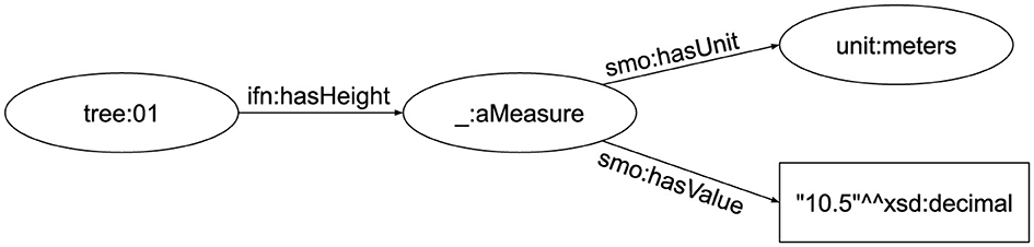
Figure 1. RDF graph.

The formal definitions of RDF triple and graph are as follows:

Definition 1 (RDF triple). Let $\mathcal{I}$, $\mathcal{B}$, and $\mathcal{L}$ be infinite disjoint sets of IRIs (Internationalized Resource Identifiers), blank nodes, and literals, respectively. An RDF triple is a tuple (s, p, o) ∈ ($\mathcal{I}$ ∪ $\mathcal{B}$) × $\mathcal{I}$×($\mathcal{I}$ ∪ $\mathcal{B}$ ∪ $\mathcal{L}$), where s is called the subject, p is the predicate, and o is the object. We write $\mathcal{T}$ the infinite set of triples.

Definition 2 (RDF graph). An RDF graph G ⊂ $2^{\mathcal{T}}$ is a set of RDF triples.

2.2 SPARQL: querying data in the Semantic Web

SPARQL (SPARQL Protocol and RDF Query Language) (Harris and Seaborne, 2013) is the W3C standard to query the RDF data model. Essentially, SPARQL is a combination of a declarative language for extracting information from RDF graphs and a protocol to send queries using the language to SPARQL processors and get the result back. The language syntax is similar to SQL, but SPARQL is based on graph pattern matching instead of relational algebra. A SPARQL query is composed of a SELECT clause listing a number of variables to be returned as results and a WHERE clause containing Basic Graph Pattern (BGP) to be matched against the RDF graph.¹ A BGP comprises a set of triple patterns: RDF triples where terms can be replaced by variables. The query returns solutions for the variables when the BGP matches an RDF subgraph substituting a variable by any term. The RDF terms for the variables are then the solution for the query. The query in Example 4 returns all possible height measures for tree:01, with their corresponding values and units. Figure 2 shows the terms and variables of the BGP matching the corresponding terms of the RDF graph in the previous example.

Example 4. SPARQL Query

      SELECT ?value ?unit

      WHERE {

         tree:01 ifn:hasHeight ?height.

         ?height smo:hasValue ?value.

         ?height smo:hasUnit ?unit.

      }

Figure 2

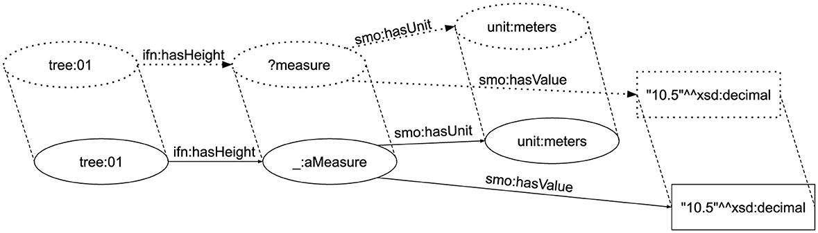
Figure 2. SPARQL graph pattern matching.

The formal definitions of SPARQL triple pattern and basic graph pattern are as follows:

Definition 3 (SPARQL Triple Pattern). Let $\mathcal{I}$, $\mathcal{B}$, $\mathcal{L}$, and $\mathcal{V}$ be infinite disjoint sets of IRIs, blank nodes, literals, and variables, respectively. A SPARQL triple pattern is a tuple (s, p, o) ∈ ($\mathcal{I}$ ∪ $\mathcal{B}$ ∪ $\mathcal{V}$) × ($\mathcal{I}$ ∪ $\mathcal{V}$) × ($\mathcal{I}$ ∪ $\mathcal{B}$ ∪ $\mathcal{L}$ ∪ $\mathcal{V}$). We write $\mathcal{P}$ the infinite set of triple patterns.

Definition 4 (SPARQL Basic Graph Pattern (BGP)). A SPARQL basic graph pattern BGP ⊂ $2^{\mathcal{P}}$ is a set of triple patterns.

BGPs are extended to SPARQL query patterns by recursively using one or more constructs that either modify the meaning of the pattern or restrict its solutions. Constructs that modify the meaning of the pattern include OPTIONAL (making part of a graph pattern facultative) and UNION (performing the logical addition of graph patterns), while constructs that restrict the solutions of the pattern are FILTER (restricting the solutions to those for that fulfill a constraint), MINUS (which removes from the solution the results from another graph pattern), and VALUES (providing a term list and restricting the solutions to those equal one of the terms).

There are currently several RDF stores that implement SPARQL, known as triplestores. A triplestore saves and indexes RDF data and provides a SPARQL endpoint: a Web address that services HTTP requests to receive queries and send back results.

The SPARQL query language has been extended to deal with domain-specific needs. Particularly relevant for this study is GeoSPARQL (Perry and Herring, 2012). GeoSPARQL defines an RDF vocabulary to express positions and polygons using either the WKT (OpenGIS, 2023) or GML (OpenGIS, 2016) serializations and a series of SPARQL functions to query spatial relationships. However, GeoSPARQL is inconsistently implemented and partially supported across triplestores (Jovanovik et al., 2021), which can lead to obtaining incorrect results (Jovanovik et al., 2021) or performance issues (Li et al., 2022).

2.3 RDFS and OWL: the semantics in “Semantic Web”

RDF Schema (RDFS) (Brickley and Guha, 2014) and the Web Ontology Language (OWL) (Hitzler et al., 2012) are semantic extensions of RDF that provide progressively higher expressivity and formal reasoning power. In addition, the vocabularies defined with RDFS and OWL help human readability and promote data reusability and interlinking (Heath and Motta, 2008).

RDFS allows to define sets of resources as Classes and describe the relationships between them. Classes and properties have an extension, that is, the set of its members (resources for classes, pairs of resources for properties), as well as intension (conceptual meaning). That means that even if two different terms are classes and have the exact same members, they can be different classes. The main elements in the RDFS vocabulary deal with:

• Class instantiation, using the rdf:type property, indicating the membership of a resource to the extension of the class.

• Class subsumption, using the rdfs:subClassOf property. If a class A is subclass of another class B, then the extension of A is a subset of to the extension of B.

• Property subsumption, using the rdfs:subPropertyOf property. If a property p is subproperty of another property q, then the extension of p is part of the extension of q.

• Property type restriction, using rdfs:domain and rdfs:range properties. If p has for domain the class A then, for every triple where p appears as predicate, the resource in the subject position is a member of class A (conversely for range and resources in the object position).

In addition, it allows to provide human-readable name and description to resources, using the rdfs:label and rdfs:comment properties. Example 5 continues our running example, shows a set of triples using the RDFS vocabulary to indicate that the tree it is indeed a tree and its species, height is a measure, and meters are a unit of measure. Figure 3 shows the graph representation of these triples.²

Example 5. RDFS triples

      tree:01 rdf:type ifn:Tree.

      tree:01 rdf:type ifn:Species01.

      _:aMeasure rdf:type ifn:Height.

      unit:meters rdf:type smo:Unit.

      ifn:Species01 rdfs:subClassOf @ifn:

          Genus01.

      ifn:Height rdfs:subClassOf smo:Measure.

      ifn:hasHeight rdfs:subPropertyOf smo:

          hasMeasure.

Figure 3

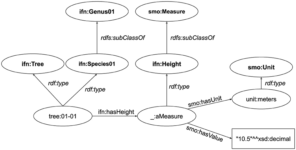
Figure 3. RDF graph with RDFS triples.

After adding these statements, the query in Example 4 can be modified to make use of these semantics and query for all measures in all existing trees, instead of only height measures of a concrete tree. This query is shown in Example 6.

Example 6. SPARQL Query using RDFS statements

      SELECT ?tree ?treeType ?measureType 

          ?value ?unit

      WHERE {

          ?tree rdf:type ifn:Tree.

          ?tree rdf:type ?treeType.

          ?tree smo:hasMeasure ?measure.

          ?measure rdf:type ?measureType.

          ?height smo:hasValue ?value.

          ?measure smo:hasUnit ?unit.

      }

OWL is an ontology language to provide formally defined meaning to Semantic Web data. It provides two alternative semantics. RDF-Based Semantics (Carroll et al., 2012), known as OWL-Full, is applicable to any RDF graph without limitations but undecidable.³ Direct Semantics (Horrocks et al., 2012), known as OWL-DL, provide semantics based on $\mathcal{S}$$\mathcal{R}$$\mathcal{O}$$\mathcal{I}$$\mathcal{Q}$ Description Logics (Horrocks et al., 2006), bringing decidability at the cost of imposing some limitations on how to use the vocabulary. OWL-DL extends $\mathcal{S}$$\mathcal{R}$$\mathcal{O}$$\mathcal{I}$$\mathcal{Q}$ with semantics for literal datatypes and Punning⁴ (Golbreich and Wallace, 2012).

An ontology is essentially a set of statements (called axioms in OWL), written using the OWL vocabulary, that are asserted to be true. A set of statements can be consistent, if all axioms in the set are true, or inconsistent, if it contains contradictory information. From a set of axioms, new statements can be inferred: A set of statements G entails a statement t iff, according to OWL semantics, whenever the all axioms in G are true, then t is true.

The OWL vocabulary reuses the RDFS vocabulary for the statements it can represent: Class instantiation, class and property subsumption, and property type restrictions. However, OWL makes explicit distinctions between classes and individuals (i.e., a resource that is an instance of a class cannot be a class itself); as well as between object properties (those that relate two individuals) and datatype properties (those that relate individuals with data values, expressed with literals in RDF). OWL has great expressivity, allowing for things such as:

• Defining classes via class equivalency (with equal intension and extension), class disjointness (making the extensions of both classes disjoint), or complex definitions: for example, as intersection, union, or complement of other classes, enumeration of individuals, or by defining a set of axioms that all the individuals in the class must have.

• Modeling property characteristics, including equivalency and disjointness (with the same meaning as classes), transitivity, bidirectionality, asymmetry, reflexiveness, or functionality.

• Expressing complex datatypes, by combining, restricting, or enumerating values of existing datatypes.

Example 7 shows a complex class definition, where a new class, smo:MeasureInMeter is defined as a measure that uses meters as units. Example 8 has two axioms. The first one defines the property smo:hasUnit as functional. This means that every individual can be linked using this property with at most one individual (i.e., if it is linked to several terms, all of them will be considered to be the same resource). The second axiom of Example 8 establishes that meters and millimeters are different units. A consequence of this is that if a set of statements included a measure with both smo:meters and smo:millimeters as its units, it would be inconsistent, since if would be inferred that both are the same individual, which contradicts the axioms that they are different.

Example 7. Complex Class Definition

      smo:MeasureInMeters rdf:type owl:Class.

      smo:MeasureInMeters rdfs:subClassOf smo:

          Measure.

      smo:MeasureInMeters owl:equivalentClass :

          _restrictionMeters.

      :_restrictionMeters rdf:type owl:

          Restriction.

      :_restrictionMeters owl:onProperty smo:

          hasUnit.

      :_restrictionMeters owl:hasValue unit:

          meters.

Example 8. Functional Property and Different Individuals

      smo:hasUnit rdf:type owl:

          FunctionalProperty.

      smo:meters owl:differentFrom smo:

          millimeters.

When using SPARQL (Section 2.2) to query RDF data described using RDFS and/or OWL, it is possible to use different entailment regimes (Glimm and Ogbuji, 2013) to redefine the evaluation of basic graph patterns of a SPARQL query according to the semantics of RDFS, OWL-DL, or OWL-Full. This allows to obtain in the results the implicit knowledge that is inferred by the chosen semantics. Note that the necessary reasoning, however, can be computationally complex (or even undecidable in the case of OWL-Full).

3 Materials and methods

The creation of the Cross-Forest Dataset involves the development of a set of ontologies to describe the data and the construction of several pipelines to read and convert the original sources into Linked Open Data. In the following subsections, we describe the original data sources (Section 3.1), the methodology used to develop the ontologies (Section 3.2), and the tools and pipelines to generate the data (Section 3.3).

3.1 Source data

The sources include long-term national forest inventories and land cover maps from Spain and Portugal. In detail, these data include the following:

The Spanish National Forest Inventory,⁵ containing statistical and sampling information of forest resources. It is updated approximately every 10 years (Bravo et al., 2002). The Spanish territory is sampled with a grid of one square kilometer cells using the UTM ED50 coordinate reference system. For each cell, a concentric plot (with radii 5, 10, 15, and 25 m and minimum tally diameter 7.5, 12.5, 22.5, and 42.5 cm, respectively) is identified and a marker placed as close to the center of the cell. Then, foresters survey each plot to sample for each tree its species, relative position (distance and bearing from the plot center), and dendrometric measures such as diameter and height. Provinces (territorial divisions similar to NUTS 3 regions) are used to organize the sampling process, as well as to provide aggregated information. The current version of this inventory (3rd IFN_es) accrues 1.4M trees and 99K plots. These data are published as a collection of 100 Microsoft Access files (two per region).

The Portuguese National Forest Inventory⁶ contains statistical (but not sampling) information of forest resources. It started in 1965 and is updated approximately every 10 years. Statistical information is published aggregated by NUTS levels 2 and 3 in Microsoft Excel files. These data are calculated from the data obtained by sampling the forest resources through the territory; however, the methodology and data from the sampling process is not disclosed by the Portuguese government. As a result, there is no information openly available about inventory plots and sampled trees in this dataset.

The Spanish Forest Map⁷ is a long-term land cover map geospatial dataset with cartographic information about forest land cover of the Spanish territory, updated every 10 years. The Spanish land cover map contains patches of terrain with similar characteristics, described using polygons over the territory. In addition to land use, each patch includes data about the dominant tree species. The boundaries and information about each patch are extracted from orthophotographies and verified through field visits to at least 20% of them. The latest version of this dataset is composed by 862.9K patches and published as a collection of 50 shapefiles (Environmental Systems Research Institute, 1998) (one per Spanish province).

The Portuguese Land Use Map⁸ is a long-term land cover map geospatial dataset with cartographic information about land cover and use (including, but not limited to, forestry uses). There are five versions of this dataset (1995, 2007, 2010, 2015, and 2018). COS contains polygons with a minimum cartographic unit of 1 ha, with a distance between lines equal to or >20 m. The data are published via a unique shapefile for mainland Portugal.

As can be seen, these datasets share some common ground, but the information is published using very different approaches: There are variations in the methodologies employed to gather the data, the published information and its level of detail, the schema and identifiers of the data, and even the format in which data are published.

3.2 Ontology development

Given the heterogeneity of the data sources to integrate (Section 3.1), we aim to create a set of ontologies for harmonizing and integrating the different sources. For this purpose, we apply some of the well-established practices in ontology development (Carmen Suárez-Figueroa et al., 2012). More specifically, we follow a bottom-up approach by first analyzing the data sources, defining the scope and the requirements.

On the one hand, each source dataset is quite valuable on its own, so the ontology should be able to describe the local particularities of each dataset. On the other hand, the ontology should cover common terms across datasets to allow transnational access to data. This leads to a modular ontology design (Abbès et al., 2012), in which we will design different ontologies to accommodate the expected uses. Hereafter, we employ the term Cross-Forest Ontology Suite to refer to the set of ontologies designed for modeling the land cover maps and forest inventories of Portugal and Spain. In the remaining of this section, we identify the different ontologies that are required, as well as specific methodologies and patterns used for building them.

One of the main goals of the Cross-Forest Ontology Suite is to facilitate its adoption and extensibility. For that, it is necessary the reuse of well-known vocabularies, as well as the connection of the data with external datasets. However, for some domains, there is a variety of vocabularies that could be potentially reused. Directly using one of those vocabularies would hamper the usability and adoption of the ontologies to part of their potential users. For this reason, we follow a pattern-based design (Hitzler et al., 2016) with indirect reuse and alignment (Lodi et al., 2017): We create local terms and patterns for all concepts and relations that can be aligned with external ontologies and vocabularies through alignment modules. Similarly, directly reusing resources from external datasets, as well as linking them without any restriction, can have reasoning implications (Halpin et al., 2010; Idrissou et al., 2017), especially (but not exclusively) if the dataset contains modeling errors. For this reason, we follow a similar approach to align resources with external datasets: We create alignment modules with different semantic implications to align individuals in the ontologies with external resources. These modules allow potential users importing the ontologies to choose their desires alignments and semantic implications.

Since all the sources contain geospatial data, we need an ontology defining common concepts for describing positions of land cover and forest inventory features (trees, plots, patches, and regions). This ontology should allow the representation of absolute and relative positions since the latter are profusely employed for positioning trees in forest inventories. Moreover, support for different coordinate reference systems is required. To the best of our knowledge, only a solution has been proposed to describe the elements of coordinate reference systems of the EPSG registry (Atemezing et al., 2014) using LOD, but the ontology is incomplete and not up-to-date, and the actual data describing the elements are not available. To design these ontologies, we make use of the Data on the Web Best Practices (Farias Lóscio et al., 2016) and Spatial Data on the Web Best Practices (Tandy et al., 2017), including the reuse of GeoSPARQL whenever possible.

Forest inventories and land cover maps also require cross-sectional ontologies for measures and tree species. An ontology of measures should allow the unambiguous identification of measurement types and their units. We design such an ontology for the Cross-Forest case by taking inspiration from QUDT⁹ and the Ontology of Units of Measure,¹⁰ with the goal of aligning the ontologies with external modules. The identification of tree species is critical for any kind of analysis involving forestry data. Biologists and taxonomists identify and classify species and higher taxa of organisms (including trees). The ontology of species should identify tree species across Cross-Forest datasets and also allow taxonomic analysis at higher taxa (genera, families, classes…) using established classifications in the field. This ontology of species is aligned with Wikidata,¹¹ DBpedia,¹² and CrossNature¹³ and includes links to Wikipedia¹⁴ and The Plant List.¹⁵

The aforementioned cross-sectional ontologies (positions, measures, and species) will be employed as building blocks for the remaining ontologies. For each dataset, we develop a dedicated ontology that is purposed to define the terminology to fully exploit each source. In this way, we aim to support those users only interested in a specific dataset. As source data are fragmented in the case of the Spanish National Forest Inventory and the Spanish Forest Map (Section 3.1), there is high value in developing local ontologies that allow uniform access to these datasets. Afterward, we create upper-level transnational ontologies for each domain (i.e., forest inventories and land use). These upper-level ontologies define the domain concepts that are specialized in the local ontologies, effectively allowing access to data at a transnational level.

In all cases, we make heavy use of metamodeling and punning (Section 2.3) to design the ontologies. This is because many of the classes need to be formally described and categorized to be used in a descriptive way, but in other cases they need to act as individuals. For example, sometimes we want to use Quercus ilex L. as an individual, when describing a specific tree species or connecting it to an external resource, while in other cases Quercus ilex is employed as a class for classifying a sampled tree with this species.

3.3 Data generation

This section provides a description of the processes by which the data from the sources presented in Section 3.1 are transformed into RDF, modeled using the ontologies described in Section 3.2.

The data generation workflow for all four datasets can be seen in Figure 4. It comprises two pipelines: (1) Preprocessing the data and (2) Generating the RDF data. In turn, each pipeline consists of several steps, depending on the dataset.

• IFN_es: The transformation of data from the Spanish National Forest Inventory starts by downloading (step 1.1) the publicly available data and decompressing it (step 1.2). Once the data are available, it is extracted to CSV (Shafranovich, 2005) (step 1.3). The results are more than a thousand CSV files that need to be preprocessed to fix errors in the data and merge files from different provinces in a single one (step 1.4). Then, the RDF data are generated from the resulting files (step 2.1). Finally, relative positions are converted to absolute positions, and WGS84 coordinates are added for each existing position (step 2.2).

• IFIS: This workflow takes the data from the Portuguese National Forest Inventory and statistical data from the Spanish National Forest Inventory to create a map with statistical information about forest resources, grouped by NUTS levels 2 and 3 for both countries. The data were gathered and stored in a Microsoft Access file during the development of the IFIS ontology; thus, the preprocessing pipeline for this data includes only extracting the data into CSV files (step 1.3). The RDF data are then generated from these files (step 2.1).

• MFE: Similarly to the IFN_es, the transformation of data from the Spanish Forest Map starts by downloading (step 1.1) the publicly available data and decompressing it (step 1.2). Then, the shapefile files are converted into GeoJSON (step 1.3), and a series of preprocessing operations generate three layers with different level of simplification and add bounding boxes for each polygon (step 1.4). Finally, each layers is transformed into RDF (step 2.1).

• COS: The shapefile files of the Portuguese Land Use Map were not publicly available during the Cross-Forest project, but they were provided by the Direção Geral do Território. Therefore, this workflow starts by extracting its content into GeoJSON (step 1.3) and performing the preprocessing to generate three layers with different levels of detail and add the bounding boxes to the polygons (step 1.4). Finally, all data are transformed into RDF (step 2.1).

Figure 4

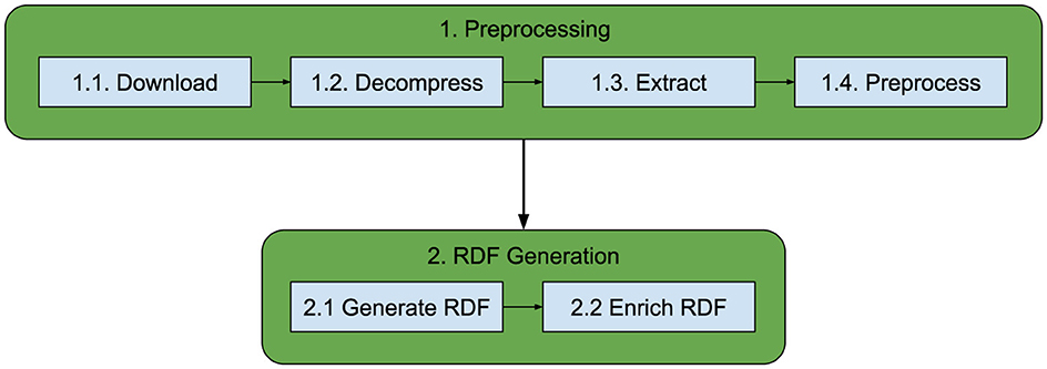
Figure 4. RDF data generation workflow.

This workflow is automatized for each dataset using a number of Bash (Fox and Ramey, 2007) scripts. These scripts make use of several tools to manipulate the data, all of which are publicly available with open licenses, whether they are existing tools or have been developed within the Cross-Forest project. The most relevant existing tools used are the following:

• UnZip (Info-ZIP Group, 2009): a Linux command-line-based extraction utility for archives compressed in.zip format. It is used to decompress data in step 1.2 of the workflow.

• MDB Tools (The MDB Tools Project, 2021): a set of libraries to manipulate database formats used by Microsoft Access and extract information from them. It is used to extract data from Microsoft Access files into CSV in step 1.3 of the workflow.

• csvtk (Shen, 2023): a Linux command-line-based tool to manipulate CSV and TSV files. It is used to merge CSV files in step 1.4 of the workflow.

• Mapshaper (Bloch, 2019): a tool for editing Shapefile, GeoJSON, TopoJSON, CSV (Shafranovich, 2005), and several other data formats, written in JavaScript. Mapshaper supports essential map making tasks such as simplifying shapes, editing attribute data, clipping, erasing, dissolving, filtering, and more. It is used to extract the data from shapefile files to GeoJSON files in step 1.3 and manipulate their content in step 1.4 of the workflow.

• SPARQL-Generate (Lefrançois et al., 2017): an extension of SPARQL 1.1 for querying not only RDF datasets but also documents in arbitrary formats. It offers a simple and expressive template-based option to generate RDF Graphs or text, from documents and different streams. It is used in step 2.1 of the workflow to generate the RDF data from either CSV or shapefile files.

In addition, epsgrdf (Gimenez-Garcıa et al., 2022) was developed as command-line tool to read RDF files that contains positions relative positions and/or absolute positions in an arbitrary CRS and generate their corresponding positions in the same CRS as the reference position, as well as in WGS84. It is used in the step 2.2 of the workflow for the IFN_es. It isv developed in Java and makes use of the following libraries:

• Apache Jena (Apache Software Foundation, 2021a): Library to extract data from, manage, and write RDF graphs. It represents the graphs as an abstract model that can be serialized in different formats.

• Apache Spatial Information System (Apache Software Foundation, 2021b): Library for developing geospatial applications. In epsgrdf, it is used to convert coordinates from one CRS to another.

• JTS Topology Suite (Eclipse Foundation, 2022): Library that provides an object model for geometries and geometric functions. In epsgrdf, it is used to read geometries from WKT strings and extract their coordinates.

The scripts, SPARQL queries, and Java source code to replicate the data generation process can be found at https://github.com/Cross-Forest/scripts, https://github.com/Cross-Forest/sparql-generate, and https://github.com/Cross-Forest/epsgrdf, respectively.

4 Results

The results of the tasks described in the previous section are the Cross-Forest Ontology Suite, described in Section 4.1, and the Cross-Forest Dataset, described in Section 4.2.

4.1 Ontologies

The Cross-Forest Ontology Suite is composed by four sets of modules. The first set are cross-sectional modules used to model measures and positions. The second and third sets are used to describe, respectively, the forest inventories and land use maps from Portugal and Spain. Finally, the fourth set is used to align terms in the previous sets with external ontologies and datasets. The ontologies and their relations can be seen on Figure 5 and are further described down below.

• Cross-sectional modules:

∘ SMO (Simple Measures Ontology): This ontology allows to characterize measures taken on entities, describing their value and their units. Its main concepts include MeasurableEntity, Measure, and Unit.

∘ EPSG (EPSG Geodetic Parameter Dataset): This ontology contains a description of existing Coordinate Reference Systems used for absolute positions, including concepts such as CoordinateSystem, Datum, and Axis.

∘ SPO (Spatial Positions Ontology): This ontology allows to represent positions of entities, whether absolute or relative to another position. Its main concepts include SpatialEntity and Position, which can be an AbsolutePosition or a Relative Position to a ReferencePosition. It makes use of SMO to model measures of positions such as distances, gradients, or areas; and of EPSG to reference Coordinate Reference Systems of positions.

• Forest Inventory modules:

∘ IFNes: This ontology allows to describe the data of the Spanish National Forest Inventory. Its main concepts include Plots, Trees, hierarchies of concepts to classify them, and dendrometric measures (reusing SMO ontology). It makes use of SPO to describe positions of plots and trees.

∘ IFIS (Iberian Forest Inventories Statistics): This ontology is used to describe the statistical data about dominant formations of the Portuguese and Spanish Inventories using a uniform schema. Its main concepts include ifi:NUTSUnit and its subclasses, ifi:NUTS1, ifi:NUTS2, or ifi:NUTS3 for NUTS areas, as well as ifi:InfoDominantFormation and ifi:InfoDominantFormationByHa.

It makes use of the SMO ontology to describe the data associated with the dominant formations.

• Land Cover Map modules:

∘ COS: This ontology allows to describe the data of the Portuguese Land Use Map. Patch and UseInPatch are its main concepts. It makes use of SPO to define the positions of the patches.

∘ MFE: This ontology allows to describe the data of the Spanish Forest Map. Its main concepts are Patch, UseInPatch, and a number of classes to define classifications and dendrometric (reusing SMO) measures about them. It uses SPO to define the positions of the patches.

∘ ILU (Iberian Land Use): This ontology contains common or generalized concepts and properties used in the Portuguese and Spanish land cover maps. Again, Patch and UseInPatch are its main concepts.

• Alignment modules: A number of modules to link terms to external ontologies and datasets. Currently used for connecting taxons with external external sources (see Section 3.2); connections to other sources will be created in future study (see Section 6). There exists two types of alignment modules:

∘ TBox modules: These modules establish subsumption and equivalence relations between classes and properties of a Cross-Forest module and an external ontology or vocabulary.

∘ Abox modules: These modules define equivalence relations between individuals in the ontologies and individuals in other datasets. There are two modules for each external dataset: one using owl:sameAs properties and the other using schema:sameAs properties.¹⁶ This allows a potential user to choose the semantic implication of these relations.

Figure 5

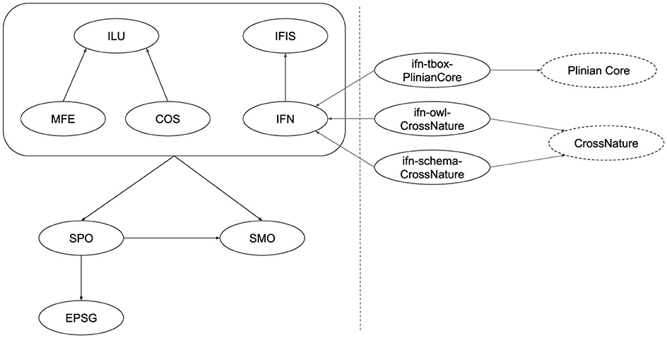
Figure 5. Cross-forest ontology suite. The right side shows an example of alignment modules with external ontologies and datasets.

All the ontologies are publicly available at https://github.com/Cross-Forest/Ontologies.

4.2 Linked Open Data

The Cross-Forest Dataset includes four separate LOD datasets, one for each of the sources described in Section 3.1. The exception being the IFN_pt, that is, combined with statistics from the IFN_es to create a combined IFIS (Iberian Forest Inventories Statistics) dataset.

The IFIS dataset includes data about the dominant formations for each NUTS 3 and NUTS 2 areas of Spain and Portugal. Figure 6 shows an instance of ifi:NUTS2 with its data about dominant formations, both absolute and relative, using individuals of type ifi:InfoDominantFormation and ifi:InfoDominantFormationByHa, respectively. These two individuals are described using the SMO ontology, using literal for their values and instances of smo:Unit for their units.

Figure 6

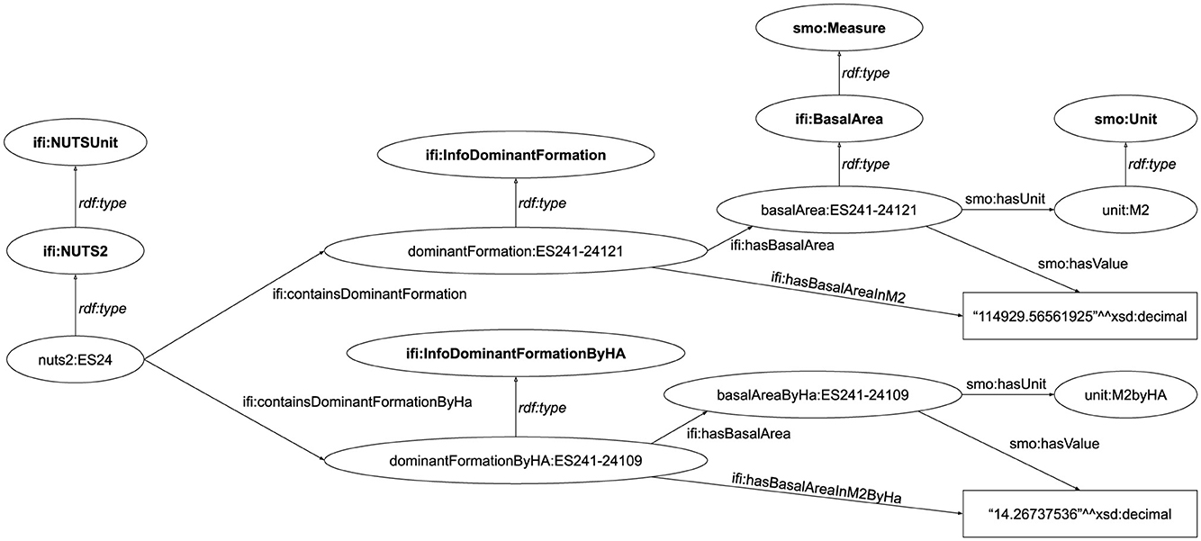
Figure 6. IFIS NUTS 2 region and example of dominant formations.

The IFNes dataset corresponds to the data of the Spanish National Forest Inventory. Its main elements are trees, plots, and measures of both. Figure 3, used as part of our running example, shows how measures for trees are modeled. The tree, instance of ifn:Tree and ifn:Species01, is connected to a measure of type ifn:Height—which is itself subclass of smo:Measure. The measure includes its value using a literal and its unit using an instance of the class smo:Unit. Note that in the figure, the shortcut to the value is missing.

Positions in the IFN_es are represented using instances of the class spo:Position, which can be Geocentric or Egocentric, using individuals of type spo:GeocentricPosition or spo:EgocentricPosition, respectively. Geocentric positions are represented using two axes and a CRS, using individuals of the classes epsg:Axisepsg:CoordinateReferenceSystem. Figure 7 shows an example of both kinds of positions. The plot has a Geocentric (i.e., absolute) position in the ED50 CRS, while the tree has its original Egocentric position, relative to the position of the plot. During the data enrichment process, a Geocentric position in ED50 is calculated for the tree, as well as positions in the WGS84 CRS (omitted from the figure for space reasons).

Figure 7

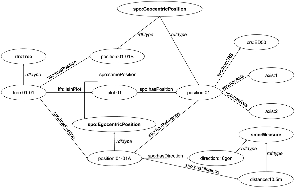
Figure 7. Positions of plots and trees in IFN_es.

The COS dataset includes the data from the Portuguese Land Use Map. Figure 8 shows an example of a patch with its associated polygon. The patch has the Use cos:Use6000, which is itself a subclass of the ILU Use ilu:TreelessLand, The position is represented by an instance of the class spo:Polygon. The position is described using a WKT string and has a bounding box defined using four individuals of type spo:Bound.

Figure 8

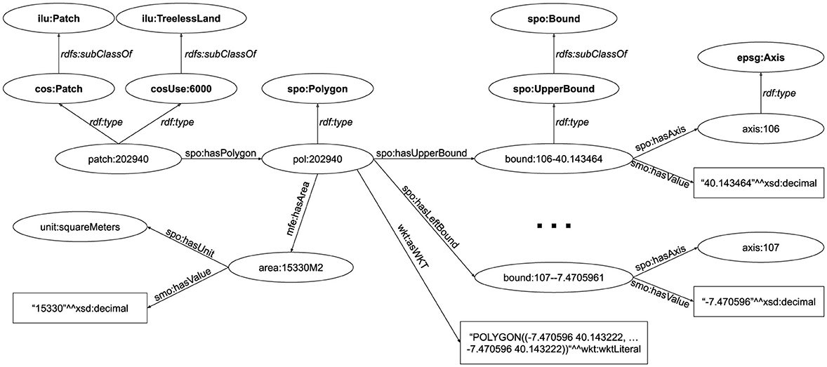
Figure 8. COS patches and positions.

The MFE dataset contains the data from the Spanish Forest Map. Its patches and polygons are modeled in identically to those on the COS (using instead the Uses defined in the MFE). In addition, it contains measures about the most abundant species in each patch, using instances of mfe:SpeciesInPatch. Figure 9 shows an example of a patch with Use mfeUse:111 and the measure about the occupation of the species.

Figure 9

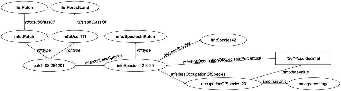
Figure 9. MFE patch and example of occupation of species.

The datasets are published at https://github.com/Cross-Forest/Data and can be queried at https://crossforest.gsic.uva.es/sparql. The data is also published in the European Data Portal (http://www.europeandataportal.eu/) and the national data portals of Portugal (https://snig.dgterritorio.gov.pt/) and Spain (https://datos.iepnb.es/def/sector-publico/medio-ambiente/). A SPARQL endpoint for the Spanish data is also available at the Spanish Natural Heritage and Biodiversity Portal (https://datos.iepnb.es/sparql/).

5 The Cross-Forest Ontology Suite and dataset in use

In this section, we showcase three different forestry scenarios where the Cross-Forest Dataset facilitates the access and use of the data. The first scenario (§5.1) presents a web-based application for easily exploring and downloading the data, contextualized in the Geres-Xures transboundary biosphere reserve. The second scenario (§5.2) presents a study that assigns inventory plots to the municipalities they belong, which in turn enables new studies at municipality level. In the third scenario (§5.3), we show how the Cross-Forest dataset simplifies feeding data to a forestry simulator, facilitating forestry management and research workflows.

5.1 Visualization of LOD with Forest Explorer

The Cross-Forest Dataset encompasses Iberian forestry inventories and land cover maps in a single resource (Section 4.2). Having an integrated dataset facilitates forest management and research activities, so that can be carried out comprehensively. Since prospective users from the forestry domain are not fluent in SW technologies, there is a need to visualize the Cross-Forest Dataset in an easy way. With this aim, we have proposed Forest Explorer.

Forest Explorer is a web application that makes the Cross-Forest Dataset accessible through an interactive map. It is developed in JavaScript to facilitate its deployment as a Web application. It is portable and can be used on any device with a modern browser (it has been successfully tested with the latest versions of Google Chrome and Mozilla Firefox on various smartphones, tablets, and personal computers). The application is publicly available at https://forestexplorer.gsic.uva.es/explorer/. Over 14K users have already employed Forest Explorer thus far. The application has been featured multiple times in the media, describing potential uses, impacts, and opportunities for forestry management. Down below, we summarize Forest Explorer and how it makes use of the Cross-Forest Dataset. More detailed information is available in its main publication (Vega-Gorgojo et al., 2022), including a different visualization forestry scenario.

The application is arranged in different components, as graphically depicted in Figure 10. The Map generator prepares the view composed of a base map (obtained from the Map server) with forestry data represented as markers, polygons, popups, or tooltips. Feature managers serve forestry data to the Map generator; there is a specialized Feature manager for each feature type: regions, land cover patches, inventory plots, and trees. The zoom level and user choices determine which Feature managers are activated. Source data are obtained from the Cross-Forest and the DBpedia endpoints, the latter providing images and multilingual descriptions of tree species. The Data manager handles such exchanges upon the receipt of a Feature manager request.

Figure 10

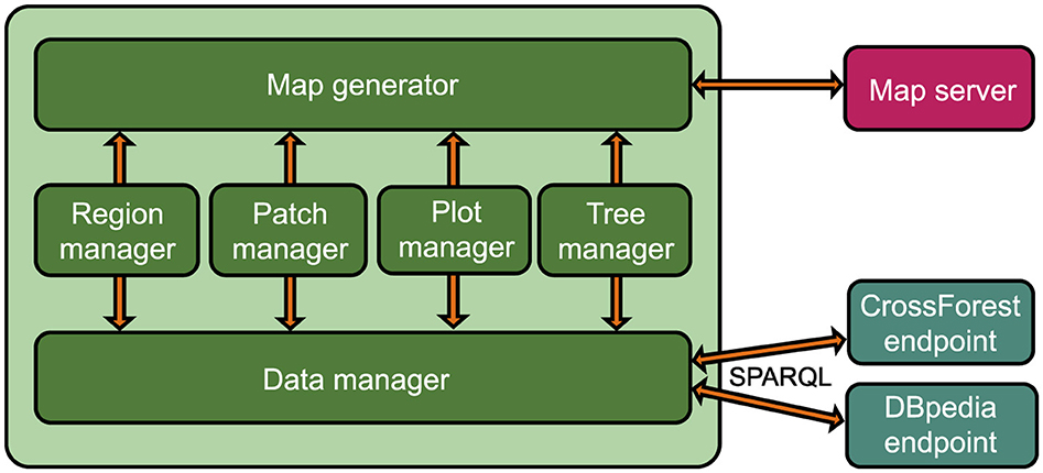
Figure 10. Architecture of forest explorer.

Figure 11 shows the user interface of Forest Explorer at different scales. The map can be easily navigated using common panning and zooming controls in both point-and-click and touch user interfaces. Zoom and positioning buttons are also included in the bottom-right; the latter centers the map in the user location. As the user navigates with the map, a Feature manager takes control by obtaining feature information from the Data manager and then sending display requests to the Map generator, as described above. For example, the Province manager controls the view of Figure 11A; the Patch manager is active in Figure 11B; the Patch and the Plot managers collaborate in Figure 11C; and the Patch and the Tree managers work together in Figure 11D.

Figure 11

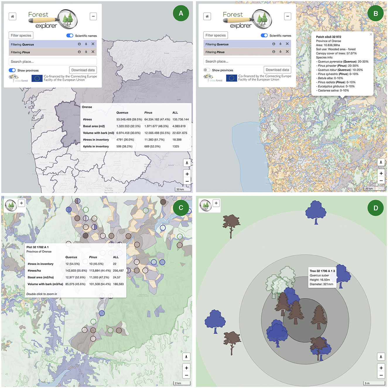
Figure 11. Snapshots of the user interface of Forest Explorer, Quercus (indigo color), and Pinus (brown) genera are filtered in all cases. (A) View of Northwest Spanish provinces and Northern Portuguese NUTS 3 regions; inventory forestry data of Orense is shown in a tooltip. (B) View of the land cover patches of Northwest Spain and North Portugal; patches are plotted in different colors depending on their use (farms in orange, water in blue, artificial in gray, and forests in green); forest patches containing a filtered species use the color filter (indigo and brown in this running example); a pop-up shows the data of a forest patch in the province of Orense. (C) View of a small forest area (see the map scale in the lower-right corner) in the Geres-Xures transboundary biosphere; Spanish plots are displayed as circles on top of the patches; plots and patches employ the same color code as before; a tooltip shows inventory data for a plot. (D) View of a tiny small forest area centered in a plot of the Geres-Xures transboundary biosphere reserve; tree markers are shown in their actual positions using taxa-dependent icons and corresponding filter colors; a tooltip shows the species, height, and diameter of a specific tree.

Although forestry data come from different sources (Section 4.2), Forest Explorer facilitates their visualization as a unified resource and hiding the intricacies of the underlying SW technologies. This is illustrated in Figure 11, displaying large areas in the Northwest part of the Iberian peninsula and zooming in into the Geres-Xures transboundary biosphere reserve (https://www.reservabiosferageresxures.eu), on the northern border of Portugal and Spain. User controls allow further adjustment of the information to display, notably taxa filters, regions/patches switch, scientific/vulgar names switch, or taxa information buttons.

Displaying Figure 11A requires gathering statistical data from the regions employed to aggregate inventory information, corresponding to Spanish provinces and Portuguese NUTS 3 regions. Example 9 includes the SPARQL query for obtaining such regions in a generic way. In a subsequent query, inventory data of each region are retrieved.

Example 9. SPARQL Query for retrieving the list of Spanish and Portuguese regions with inventory data

  PREFIX ifn:  <https://datos.iepnb.es/def/

     sector-publico/medio-ambiente/ifn/>

  PREFIX ifi:  <http://crossforest.eu/ifi/

     ontology/>

  PREFIX country:  <http://crossforest.eu/ifi/

     data/country/>

  SELECT DISTINCT ?region {

    {

      ?region a ifn:Province.

    } UNION {

      ?region a ifi:NUTS3;

         ifi:isInCountry country:PT.

    }

  }

In the case of Figure 11B, we need to obtain the patches in the map view. The SPARQL query in Example 10 serves for this purpose; it specifies a bounding box with WGS84 coordinates −8.2W 42.0N −8.2E 41.6S (covering Geres-Xures). Target patches enclose polygons that are included or intersect such bounding box. The query includes the selection of layer ilu:s5s5 (defined in ILU Section 4.1) to allow the retrieval of Spanish and Portuguese patches.

Example 10. SPARQL Query for retrieving the Iberian patches with polygons that are included or intersect the bounding box with WGS84 coordinates −8.2W 42.0N −8.2E 41.6S

    PREFIX pos:  <http://crossforest.eu/

       position/ontology/>

    PREFIX epsg:  <http://epsg.w3id.org/

       ontology/>

    PREFIX ilu:  <http://crossforest.eu/ilu/

       data/layer/>

    SELECT DISTINCT ?patch ?poly WHERE {

     ?patch pos:hasPolygon ?poly.

     ?poly epsg:hasLeftBound107 ?west;

       epsg:hasRightBound107 ?east;

       epsg:hasUpperBound106 ?north;

       epsg:hasLowerBound106 ?south;

       pos:isInLayer ilu:s5s5.

     FILTER (?south  <= 42.0)

     FILTER (?north >= 41.6)

     FILTER (?west  <= -7.9)

     FILTER (?east >= -8.2)

    }

For the retrieval of the plots in Figure 11C, we use a very similar SPARQL query. In this case, plot data come from IFN_es. Example 11 serves to obtain the plots with a location included in the same bounding box as before.

Example 11. SPARQL Query for retrieving the IFN_es plots inside the bounding box with WGS84 coordinates −8.2W 42.0N −8.2E 41.6S

    PREFIX ifn:  <https://datos.iepnb.es/def/

       sector-publico/medio-ambiente/ifn/>

    PREFIX pos:  <http://crossforest.eu/

       position/ontology/>

    PREFIX crs:  <http://epsg.w3id.org/data/crs

       />

    PREFIX axis:  <http://epsg.w3id.org/

       ontology/axis/>

    SELECT ?plot ?lat ?lng WHERE {

      ?plot a ifn:Plot;

        pos:hasPosition ?pos.

      ?pos pos:hasCoordinateReferenceSystem crs

          :4326;

        axis:106 ?lat;

        axis:107 ?lng.

      FILTER (?lat  <= 42.0)

      FILTER (?lat >= 41.6)

      FILTER (?lng  <= -7.9)

      FILTER (?lng >= -8.2)

    }

After obtaining the plots in the map view, it makes sense to display the sampled trees if the zoom level is high enough. The SPARQL query in Example 12 is used to obtain the trees (with their positions) that were sampled for plot:32-1796-A-1, that is, the plot shown in Figure 11D.

Example 12. SPARQL Query for retrieving the trees and positions of plot:32-1796-A-1

    PREFIX ifn:  <https://datos.iepnb.es/def/

       sector-publico/medio-ambiente/ifn/>

    PREFIX plot:  <https://datos.iepnb.es/

       recurso/sector-publico/medio-ambiente/

       ifn/plot/>

    PREFIX pos:  <http://crossforest.eu/

       position/ontology/>

    PREFIX crs:  <http://epsg.w3id.org/data

       /crs/>

    PREFIX axis:  <http://epsg.w3id.org/

       ontology/axis/>

    SELECT DISTINCT ?tree ?lat ?lng WHERE {

     ?tree a ifn:Tree;

       ifn:isInPlot plot:32-1796-A-1;

       pos:hasPosition ?pos.

     ?pos pos:hasCoordinateReferenceSystem crs

         :4326;

       axis:106 ?lat;

       axis:107 ?lng.

    }

The application includes a “Download data” button (see Figure 11A) that can be used to obtain the data displayed in the view. In this way, the user can obtain land cover patches, forest inventory plots, and trees of the area of interest (the Geres-Xures transboundary biosphere reserve in this case). Note that Forest Explorer can be used to visualize forestry data for any area in Spain or Portugal, extending beyond the example presented here.

5.2 Automatic assignment of forest inventory plots to municipalities

An integrated forestry inventory offers several advantages for forest management, such as facilitating informed decision-making, research, and woodland analyses at local level. Local Administrative Units (LAUs) cover the entire territory without overlap and are nested within higher-level LAUs such as counties or provinces, enabling information upscaling. They also follow a standardized nomenclature compatible with NUTS (LAUs are a subdivision of NUTS 3).

In the case of Spain, municipalities are the relevant LAUs for forest management. Unfortunately, the IFN_es contains missing and unreliable information regarding plot municipalities that preclude their use in practice. Since the National Geographic Institute¹⁷ publishes a geospatial dataset of Spanish municipalities with their boundaries, it should be possible to obtain the municipality of each plot by combining data from the inventory and municipalities datasets. However, this process using the original IFN_es data would involve many cumbersome and error-prone tasks to preprocess and align their data.

In this subsection, we summarize how this process was simplified by using the Cross-Forest Dataset in Crespo-Lera et al. (2023). In this study, the IFN_es plots were assigned to Spanish municipalities. We used three different workflows to cross-validate the results and identify the optimal one for similar future studies. Note that we include here some methodological guidelines that are part of this study. For more methodological and technical details, see Crespo Lera (2023). In addition, we show an example of how this result can be used for further studies at local level, by producing a map with the dominant tree species for each Spanish municipality.

In a first stage, we designed a small municipality ontology that defined the necessary terms for expressing the municipality dataset into RDF. We adapted the data generation workflow in Section 3.3 for making the conversion of the source data, originally in Shapefile format. As a result, we obtained an RDF graph with the 8,131 Spanish municipalities and their corresponding geometries (polygons or multipolygons).

Next, we employed a Geographical Information System, QGIS, and two triplestores, Virtuoso and Fuseki, to automatically compute the assignments of plots to municipalities. In the case of QGIS, we used the Join attributes by location tool to determine whether a plot geometry (point) is contained within another geometry (municipality boundaries). Regarding the triplestores, we prepared a SPARQL query with the sfWithin function, which identifies if a plot is entirely contained within a municipal geometry. We found that QGIS and Fuseki obtained the same plot-municipality assignment that was assessed as correct after several tests. The outcome of Virtuoso was discarded due to a problem with false positives.¹⁸

The resulting integration of datasets facilitates the extraction of comprehensive local-level information, encompassing crucial metrics such as municipalities without plots, the mean number of inventory plots, dominant species per municipality, and the count of mixed and pure plots within these local units. As an illustrative example, the SPARQL query in Example 13 calculates the mean basal area (m²/ha) for each species in every Spanish municipality. This information was employed to generate maps displaying dominant species per municipality, offering a fairly accurate reflection of species distribution across Spain (Figure 12). Zou et al. (2019) describe this use case in more depth.

Figure 12

Figure 12. Map example showing dominant species by municipality in Spain, created using the integrated dataset with data from the third edition of the Spanish National Forest Inventory and municipal boundaries.

Using IFN_es LOD-integrated data alongside municipal boundaries, we developed a map revealing the dominant tree species across Spanish municipalities. By analyzing basal area data from IFN_es plots across all forested regions, this map offers a comprehensive description of Spain's forest ecosystems at a local scale. It highlights the primary tree species in various regions of the Peninsula, showcasing the country's rich biodiversity with 59 dominant species identified across 6,056 forest municipalities.

This map serves as a valuable resource for several reasons. It offers a clear view of tree species distribution across municipalities, empowering local authorities and forest managers to make informed decisions on conservation, resource management, and comparing biodiversity within their regions. Furthermore, the detailed, municipality-level data serve as a tool for researchers studying forest ecosystems and policymakers shaping forestry strategies, among others.

Example 13. SPARQL Query for obtaining the mean basal area (m²/ha) for each species in every Spanish municipality

    PREFIX ifn:  <https://datos.iepnb.es/def/

       (sector-publico/medio-ambiente/ifn/>

    SELECT ?muni ?species AVG(?G) as ?meanG

        WHERE {

     ?plot a ifn:Plot;

       ifn:containsSpeciesPlot 

           ?infoSpeciesPlot;

       ifn:isInMunicipality ?muni.

     ?infoSpeciesPlot ifn:hasBasalAreaInM2byHA 

         ?G;

       ifn:hasSpecies ?species.

    }

    GROUP BY ?muni ?species

    ORDER BY ?muni desc(?meanG)

5.3 SIMANFOR: LOD-based simulation of forests

The Spanish National Forest Inventory is used in many forest research activities in Spain. However, using the officially published data in its original format is inconvenient, forcing researchers to perform ad hoc data preprocessing to adapt it to their needs. Here, we show one of such research activities—forecasting the impact of silvicultural actions on forest dynamics—where the Cross-Forest Dataset simplifies the use of IFN_es data in their research.

SIMANFOR (https://www.simanfor.es) is a forestry simulator that can be used for management and planning activities (Bravo et al., 2012). This simulator uses forest inventory data as initial state and combines forest growth and yield models defined by user silvicultural actions (thinning and harvesting) to forecast forest dynamics at stand and tree level. SIMANFOR projects ingrowth, mortality, and growth, yielding valuable outputs such as size distribution, volume, and biomass, which are essential for informed decision-making in forestry management and planning.

One drawback of SIMANFOR and other competing simulators lies in the rather demanding process required for preparing input data, which severely hinders research activities and limits both their utility and their potential audience. For example, using a scenario based on (Riofrío et al., 2017), suppose that we want to simulate the effects of different silvicultural actions as thinnings (with different timing and intensity) in mixed forests of Pinus sylvestris L. and Pinus pinaster in “Sierra de la Demanda” using available inventory data in the Spanish National Forest Inventory. While SIMANFOR is especially suitable for running this type of simulations, gathering and formatting the input data is quite problematic. “Sierra de la Demanda” is a mountain sub-range situated in northern Spain that comprises three provinces (Burgos, La Rioja, and Soria). Since the Spanish National Forest Inventory publishes two Microsoft Access files per province, this case requires loading six different databases, then extracting the suitable plots from each database, integrating the results, and finally converting them to a format suitable for SIMANFOR. This is not only cumbersome, but it also requires a suitable computing environment with a Microsoft Access license, non-trivial database skills, and good knowledge of the schema and ID codes used in the databases.

Instead, the endpoint of the Cross-Forest Dataset can be used to gather the data of interest. In a first step, we can prepare a SPARQL query for obtaining the pure Pinus sylvestris (ifn:Species21) plots located in the provinces of Burgos, La Rioja, and Soria with latitudes between WGS84 42.5 and 41.5. This combination of administrative and latitude restrictions roughly corresponds to “Sierra de la Demanda”.¹⁹ Example 14 includes such SPARQL query and can be run by pasting it at https://crossforest.gsic.uva.es/sparql.

Example 14. SPARQL Query for finding the pure Pinus sylvestris (ifn:Species21) plots in the provinces of Burgos, La Rioja, and Soria with latitudes between WGS84 42.5 and 41.5

  PREFIX ifn:  <https://datos.iepnb.es/def/

     sector-publico/medio-ambiente/ifn/>

  PREFIX ter:  <http://vocab.linkeddata.es/

     datosabiertos/def/sector-publico/

     territorio\#>

  PREFIX rdfs:  <http://www.w3.org/2000/01/rdf

     -schema\#>

  PREFIX pos:  <http://crossforest.eu/position

     /ontology/>

  PREFIX crs:  <http://epsg.w3id.org/data/

     crs/>

  PREFIX axis:  <http://epsg.w3id.org/ontology

     /axis/>

  

  SELECT DISTINCT ?plot WHERE {

   # plots with any Pinus sylvestris

   ?plot a ifn:Plot.

   ?tree1 ifn:isInPlot ?plot;

     a ifn:Species21.

 

   # located in provinces Burgos, La Rioja, or 

        Soria

   VALUES ?prlab { ‘‘Burgos’’@es ‘‘La Rioja’’

        @es ‘‘Soria’’@es  }

   ?plot ter:provincia ?pr.

   ?pr rdfs:label ?prlab.

 

   # with latitudes between WGS84 42.5 

      and 41.5

   ?plot pos:hasPosition ?pos.

   ?pos pos:hasCoordinateReferenceSystem crs:

      4326;

     axis:106 ?lat.

   FILTER (?lat  <= 42.5)

   FILTER (?lat >= 41.5)

 

   # only pure plots

   FILTER NOT EXISTS {

    ?tree2 ifn:isInPlot ?plot.

    FILTER NOT EXISTS {?tree2 a ifn:Species21 

         }

   }

  }

Obtaining the pure Pinus pinaster (ifn:Species26) plots in “Sierra de la Demanda” can be trivially carried out by replacing ifn:Species21 with ifn:Species26 in the previous snippet. Next, we can obtain the mixed Pinus sylvestris and Pinus pinaster plots with the SPARQL query in Example 15.

Example 15. =SPARQL Query for obtaining the list of mixed plots of Pinus sylvestris (ifn:Species21) and Pinus pinaster (ifn:Species26) in the provinces of Burgos, La Rioja, and Soria with latitudes between WGS84 42.5 and 41.5

  PREFIX ifn:  <https://datos.iepnb.es/def/

     sector-publico/medio-ambiente/ifn/>

  PREFIX ter:  <http://vocab.linkeddata.es/

     datosabiertos/def/sector-publico/

     territorio\#>

  PREFIX rdfs:  <http://www.w3.org/2000/01/rdf

     -schema\#>

  PREFIX pos:  <http://crossforest.eu/position

     /ontology/>

  PREFIX crs:  <http://epsg.w3id.org/data/

     crs/>

  PREFIX axis:  <http://epsg.w3id.org/ontology

     /axis/>

 

  SELECT DISTINCT ?plot WHERE {

   # plots with any Pinus sylvestris and any 

       Pinus pinaster

   ?plot a ifn:Plot.

   ?tree1 ifn:isInPlot ?plot;

     a ifn:Species21.

   ?tree2 ifn:isInPlot ?plot;

     a ifn:Species26.

 

   # located in provinces Burgos, La Rioja, or 

        Soria

   VALUES ?prlab { ‘‘Burgos’’@es ‘‘La Rioja’’

        @es ‘‘Soria’’@es  }

   ?plot ter:provincia ?pr.

   ?pr rdfs:label ?prlab.

   # with latitudes between WGS84 42.5 and 41

       .5

   ?plot pos:hasPosition ?pos.

   ?pos pos:hasCoordinateReferenceSystem crs:

       4326;

    axis:106 ?lat.

   FILTER (?lat  <= 42.5)

   FILTER (?lat >= 41.5)

 

   # no other trees that are not Pinus 

       sylvestris or pinaster

   FILTER NOT EXISTS {

     ?tree3 ifn:isInPlot ?plot.

     FILTER NOT EXISTS {?tree3 a ifn:Species21 

         }

     FILTER NOT EXISTS {?tree3 a ifn:Species26 

         }

   }

  }

The previous queries serve to obtain the list of plots that comply with the selection requirements. In a next stage, a query is employed for extracting plot data (geocoordinates, height, slope, and age) and another one for obtaining their sampled trees and associated data (position, diameter, height, species, expansion factor, and tree status). Obtained data are then converted to CSV, the native input format of SIMANFOR. In this way, end users do not longer need to manually prepare an input file for running a simulation with SIMANFOR.

In the study in which this scenario is based (Riofrío et al., 2017), the presented workflow could have been applied to retrieve the data, considerably easing the effort of the whole research endeavor. Other publications could also have benefited by using the Cross-Forest dataset to simplify their data gathering processes: Herrero et al. (2019) used SIMANFOR to simulate different management and climate scenarios to predict mushroom production in Pinus pinaster Ait. ecosystems in northern Spain, finding that silvicultural treatments had a positive influence. Rodriguez de Prado et al. (2023) used SIMANFOR to simulate CO2 stock evolution from 2000 to 2100 in pure and mixed stands of most representative species under different silvicultural scenarios. Vázquez-Veloso et al. (2023) evaluated the accuracy of the IBERO growth and yield model by comparing the simulations of pure stand plots of Pinus pinaster and Pinus sylvestris from different versions of the Spanish National Forest Inventory. While these studies required a considerable effort in data preparation, similar future studies can instead rely on the Cross-Forest Dataset to simplify their tasks.

We are currently working in a new version of SIMANFOR that automatically consumes LOD from the Cross-Forest Dataset. As SIMANFOR end users do not typically know SPARQL, we are developing a web interface for selecting inventory plots. Specifically, it will be possible to draw the target area in a map and then set different constraints (taxa, number of trees, and so on). Obtained plots will be shown to users, allowing them to go on with the simulation in a next stage or to go back and refine their selection constraints.

6 Discussion

This study presents the Cross-Forest Dataset, a knowledge graph representation of the Portuguese and Spanish Forest Inventories and Land Use Maps, and the Cross-Forest Ontology Suite, a formal description of the entity concepts and relations that exist in the data. The flexible structure of the knowledge graph allows to easily integrate the different sources, connect them with external data, and query everything in an uniform way. The ontologies bring the reasoning capabilities of Knowledge Representation and Reasoning, a field of artificial intelligence that adds formal semantics to the data. This allows for tasks such as evaluating the consistency and completeness of the data, making logical inferences of implicit knowledge, classifying data, and assisting other AI fields such as problem solving (Bouzid et al., 2012), natural language processing (Maynard et al., 2017), rule-based systems (Rattanasawad et al., 2018), neuro-symbolic AI (Hitzler et al., 2023), large language models (Ye et al., 2023), or explainability in AI (Rajabi and Etminani, 2022).

The Cross-Forest Dataset provides a single endpoint for accessing forestry data. This is quite convenient since the source datasets are available in different formats and technologies or even fragmented in multiple databases as the Spanish National Forest Inventory. In this way, it is possible to pose arbitrary queries that make use of the different sources through the Cross-Forest endpoint. Note that data integration is one of the main challenges of forestry science, as reported in many studies such as Zou et al. (2019). The Cross-Forest Dataset thus illustrates how the use of Semantic Web technologies and Linked Open Data principles can be applied to address this challenge.

Over the last two decades, experts and managers of National Forest Inventories in 23 European countries, in the framework of the group “European National Forest Inventory Network” (ENFIN), have devoted lots of efforts toward harmonization in reporting assessment of forest resources. Every cycle of inventory across this area has over half million plots, with different methodologies, techniques, definitions, and type of information gathered (Vidal et al., 2016). LOD strategies followed in Cross-Forest project can enhance efforts to obtain comparable data that can be aggregated at European level.

Biomass as energy resource has became a crucial importance over the world. At European level, simulations with EFISCEN model (Verkerk et al., 2019) have estimated theoretical amount of biomass in the current situation and the evolution over next decades, based on data from NFI of each country. Puliti et al. (2021) estimated above-ground net change of biomass based on NFI and satellite imagery in Norway. At African level, Vaglio Laurin et al. (2014) used small footprint LiDAR metrics to estimate biomass stocks, while at a global scale, Hu et al. (2016) used LiDAR techniques to asses forest above-ground biomass estimations. GEDI mission,²⁰ on the ISS from 2018 to 2023, will add further high resolution laser ranging observations of the 3D forest structure improving the characterization of carbon and water cycling processes, biodiversity, and habitat. A challenge ahead is the integration of such information with LOD. This multi-scale interest in biomass demonstrates the opportunity of LOD techniques to favor the efforts devoted all around the world.

Tang et al. (2015) proposed a tool to simulate plant growth processes that integrates an ontology, artificial intelligence, and virtual plant techniques. They focus on the Chinese fir, collecting a large amount of existing information on the growth and development patterns and then construct an ontology to organize the information. This virtual environment illustrates the usage of Semantic Web technologies in the forestry sector.

Visualization is an immediate application case of an integrated forestry dataset as it enables end users to analyze large amounts of complex data, for example, for forestry management (Zou et al., 2019). Geographical Information Systems (GISs) are commonly employed for visualizing forestry data; Global Forest Watch²¹ is a well-known example. Note that GISs do not rely on LOD and use instead their own formats. As a result, the integration of external datasets into a GIS is time-consuming and complex (Lehmann et al., 2015). In contrast, the Forest Explorer (Section 5.1) is a web application that consumes LOD from the Cross-Forest Dataset. Since this dataset is interlinked to external sources, for example, species thesauri from Wikidata and DBpedia, Forest Explorer exploits this to display additional species information such as images and textual descriptions that are not available in the Cross-Forest Dataset. So far, more than 14K users have employed Forest Explorer in 25K different sessions (we employed Google Analytics²² to keep track of the usage of the application). Importantly, the exploitation of LOD is hidden from end users, while the choice of technologies facilitates its usage even with off-the-self smartphones. Nevertheless, other viewers can be developed that improve the Forest Explorer or that provide alternative capabilities, benefiting from the usage of LOD and open standards.

Beyond visualization, the Cross-Forest Dataset can be exploited in different ways for addressing forestry domain problems. The project in Section 5.2 showcases the integration of a municipality dataset to derive new data (the assignment of forestry plots to municipalities) and new insights (dominant tree species per municipality at national level). These types of studies are difficult to conduct with traditional database technologies, so they are typically restricted to narrow areas (Rescia et al., 2008; Farias Arquer and Valderrábano Luque, 2007).

The case of SIMANFOR (Section 5.3) illustrates another application of the Cross-Forest Dataset. Data preparation is a demanding, time-intensive, and error-prone task. Fortunately, forestry LOD can be employed to discharge end users from this responsibility. In this way, SPARQL queries, such as the ones in Examples 14–15, can be formulated to express complex plot selection criteria. Since knowledge of SPARQL cannot be assumed for forestry domain experts, we are working on the design of a web interface to simplify this process. Note that visualizations are typically employed with LOD and SW technologies to address data access (Vega-Gorgojo et al., 2016, 2019; Soylu et al., 2016).

By developing ad hoc solutions or integrating external solutions such as nFIESTA,²³ we could obtain sound estimates of target parameters (biomass, carbon…) at both static and dynamic levels. nFIESTA, developed under the EU's H2020 DIABOLO project,²⁴ is currently a sound option to gain insight on forest estimations from the Cross-Forest Dataset. However, more in-depth analysis is needed to calibrate the integration of nFIESTA capability with our LOD workflow.

The forest sector faces unprecedented challenges in managing forest ecosystems in the context of climate change. Foresters need on-time, accurate, and easy to digest information about forests and its structure to plan and conduct proper management. Therefore, having access to robust databases enriched with high-quality data that reflect the conditions (structure complexity, mixing degree...) and evolution including stand dynamic (tree and stand growth, ingrowth, and mortality/survival), area expansion (agricultural land abandonment...), reduction (by illegal logging, fire occurrence...), or degradation of forest areas, and that allow them to simulate various alternatives and scenarios, is an invaluable tool on which they can base informed decision-making. In addition, our study extends its benefits to non-expert users, including data journalists and interested citizens. It simplifies the visualization of integrated forest databases, making forest-related information more accessible.

This study is part of an living project, with several ongoing tasks. First, we want to align the Cross-Forest Ontology Suite with several well-known ontologies [such as the Darwin Core Task Group, 2009 for species; the ISA Programme Location Core Vocabulary (Barthelemy et al., 2004) and the Basic RDF Geo Vocabulary (Brickley, 2006) for positions; and QUDT (Hodgson et al., 2014), the Semantic Sensor Network Ontology (Haller et al., 2017), and the Ontology of Units of Measure (Rijgersberg et al., 2013) for measures]. Second, we are working on adding the temporal dimension to the Spanish, by integrating the previous and upcoming versions of the Forest Inventory and Land Use Map. Third, we plan to incorporate new resources to the data, starting with LiDAR (Liang et al., 2022) and climate data. Finally, we are upgrading Simanfor to be able to directly query the Cross-Forest Dataset and writing its results in RDF. This will bring the ability to have reusable and shareable intermediate results that can be uniformly queried and used as intermediate results for new predictions or simulations.

Note that the current ontologies aim to describe the Portuguese and Spanish Forestry data, but they have been developed with the goal of being generalizable and extensible for international use. We expect to integrate data of other countries in the foreseeable future.

Data availability statement

The ontologies, datasets, and tools to replicate the data generation process presented in this study can be found in online repositories and SPARQL query endpoints. The names of the repositories/endpoints and their URLs can be found in the article.

Author contributions

JG-G: Data curation, Formal analysis, Investigation, Methodology, Software, Validation, Writing – original draft, Writing – review & editing. GV-G: Conceptualization, Funding acquisition, Investigation, Project administration, Software, Supervision, Validation, Visualization, Writing – review & editing. CO: Formal analysis, Investigation, Writing – review & editing. NC-L: Data curation, Investigation, Software, Writing – review & editing. FB: Conceptualization, Funding acquisition, Project administration, Resources, Supervision, Validation, Writing – review & editing.

Funding

The author(s) declare financial support was received for the research, authorship, and/or publication of this article. This study has been partially funded by the European Commission through Cross-Forest (2017-EU-IA-0140) and Spanish Ministry of Science and Innovation through LOD.For.Trees (TED2021-130667B-I00), IMFLEX (PID2021-1262750B-C22), and H20 (PID2020-112584RB-C32) projects and by the Junta de Castilla y León through CLU-2019-01 and CL-EI-2021-05—iuFOR Institute Unit of Excellence of the University of Valladolid, co-financed by the European Regional Development Fund (ERDF “Europe drives our growth”).

Acknowledgments

The authors would like to thank Grupo Tragsa, Direção-Geral do Território (DGT—Portugal), Fundación Centro de Supercomputación Castilla y León (SCAYLE), and Ministerio para la Transición Ecológica y el Reto Demográfico (MITECO—Spain) for their support during the Cross-Forest project.

Conflict of interest

The authors declare that the research was conducted in the absence of any commercial or financial relationships that could be construed as a potential conflict of interest.

The author(s) declared that they were an editorial board member of Frontiers, at the time of submission. This had no impact on the peer review process and the final decision.

Publisher's note

All claims expressed in this article are solely those of the authors and do not necessarily represent those of their affiliated organizations, or those of the publisher, the editors and the reviewers. Any product that may be evaluated in this article, or claim that may be made by its manufacturer, is not guaranteed or endorsed by the publisher.

Footnotes

1. ^Similarly to SQL, several constructors can be applied to the WHERE clause.

2. ^Note that, for all document figures, Classes are written in bold and schema properties (from RDFS and OWL) are written in italic.

3. ^A logical system is decidable if it is always possible to either decide if a set of axioms is consistent or not and infer all possible knowledge in limited time.

4. ^A metamodeling capability that allows to use the same term for a class and an individual, essentially allowing to describe classes using arbitrary properties.

5. ^Inventario Forestal Nacional, Available at: https://www.miteco.gob.es/es/biodiversidad/servicios/banco-datos-naturaleza/informacion-disponible/ifn3.aspx.

6. ^Inventário Florestal Nacional, Available at: https://icnf.pt/florestas/flestudosdocumentosestatisticasindicadores.

7. ^Mapa Forestal Español, Available at: https://www.miteco.gob.es/es/biodiversidad/servicios/banco-datos-naturaleza/informacion-disponible/mfe50.aspx.

8. ^Carta de Ocupação do Solo, Available at: https://smos.dgterritorio.gov.pt/cartografia-de-uso-e-ocupacao-do-solo.

9. ^https://www.qudt.org/

10. ^https://www.ebi.ac.uk/ols/ontologies/om

11. ^https://www.wikidata.org/

12. ^https://www.dbpedia.org/

13. ^https://crossnature.eu/

14. ^https://www.wikipedia.org/

15. ^http://www.theplantlist.org/

16. ^The owl:sameAs relation implies semantic equality of the two individuals, meaning that whenever one of them is the subject or object of any triple, it is inferred an equivalent triple using the other. The schema:sameAs relation does not have any semantics and is used to only convey this equality information to users of the data.

17. ^https://www.ign.es

18. ^We opened an issue at the Virtuoso GitHub repository: https://github.com/openlink/virtuoso-opensource/issues/1098.

19. ^Another plausible alternative is to specify the geometry of the polygon and then calculate the pure plots ofPinus sylvestris contained in such polygon using the GeoSPARQL st_within function.

20. ^https://gedi.umd.edu

21. ^https://www.globalforestwatch.org

22. ^https://marketingplatform.google.com/about/analytics/

23. ^https://gitlab.com/nfiesta

24. ^http://diabolo-project.eu/

References

Abbès, S. B., Scheuermann, A., Meilender, T., and d'Aquin, M. (2012). “Characterizing modular ontologies,” in Proceedings of the 6th International Workshop on Modular Ontologies (Graz: WoMo), 13–25. Available at: https://hal.science/docs/00/73/61/89/PDF/WoMo_paper_2012_SBA_al.pdf (accessed October 10, 2023).

Google Scholar

Apache Software Foundation (2021a). Apache Jena. Available at: https://jena.apache.org/ (accessed September 02, 2024).

Google Scholar

Apache Software Foundation (2021b). Apache Spatial Information System. Available at: https://sis.apache.org/ (accessed September 02, 2024).

Google Scholar

Atemezing, G., Abadie, N., Troncy, R., and Bucher, B. (2014). “Publishing reference geodata on the web: opportunities and challenges for IGN France,” in Terra Cognita 2014, 6th International Workshop on the Foundations, Technologies and Applications of the Geospatial Web. In Conjunction with the 13th International Semantic Web Conference (Riva del Garda).

Google Scholar

Barthelemy, F., Beaufays, A., De Keyzer, M., Fragkou, P., Schepers, D., Stani, E., et al. (2004). Core Location Vocabulary. Available at: https://semiceu.github.io/Core-Location-Vocabulary/releases/2.0.2/ (accessed September 02, 2024).

Google Scholar

Berners-Lee, T., Fielding, R., and Masinter, L. (2005). Uniform Resource Identifier (URI): Generic Syntax. Available at: https://datatracker.ietf.org/doc/html/rfc3986 (accessed September 02, 2024).

Google Scholar

Berners-Lee, T., Masinter, L., and McCahill, M. (1994). Uniform Resource Locators. Available at: http://tools.ietf.org/html/rfc1738 (accessed September 02, 2024).

Google Scholar

Bizer, C., Vidal, M.-E., and Skaf-Molli, H. (2018). “Linked open data,” in Encyclopedia of Database Systems, eds. L. Liu and M. T. Ösu (New York, NY: Springer), 2096–2101.

Google Scholar

Bloch, M. (2019). Mapshaper. Available at: https://github.com/mbloch/mapshaper (accessed September 02, 2024).

PubMed Abstract | Google Scholar

Bouzid, S., Cauvet, C., and Pinaton, J. (2012). “A survey of semantic web standards to representing knowledge in problem solving situations,” in Proceedings of the 2012 International Conference on Information Retrieval & Knowledge Management, 121–125. Available at: https://ieeexplore.ieee.org/abstract/document/6205018 (accessed October 25, 2023).

Google Scholar

Bravo Oviedo, F., Ordóñez Alonso, C., and Lara Henao, W. (2022). “basifoR: paquete de r para manejar los datos del inventario forestal nacional,” in VIII congreso forestal español (Lleida: Sociedad Española de Ciencias Forestales).

Google Scholar

Bravo Oviedo, F., Rivas González, J., Monreal Núñez, J., and Ordóñez Alonso, C. (2004). BASIFOR 2.0: Aplicación informática para el manejo de las bases de datos del inventario forestal nacional. Cuadernos Soc. Española Cienc. For. 18, 243–247. doi: 10.31167/csef.v0i18.9466

Crossref Full Text | Google Scholar

Bravo, F., del Río, M., and del Peso, C., (eds.). (2002). El inventario forestal nacional. Elemento clave para la gestión forestal sostenible. Valladolid: Fundación General de la Universidad de Valladolid.

Google Scholar

Bravo, F., Fabrika, M., Ammer, C., Barreiro, S., Bielak, K., Coll, L., et al. (2019). Modelling approaches for mixed forests dynamics prognosis. research gaps and opportunities. For. Syst. 28:eR002. doi: 10.5424/fs/2019281-14342

Crossref Full Text | Google Scholar

Bravo, F., Rodríguez, F., and Ordoñez, C. (2012). A web-based application to simulate alternatives for sustainable forest management: SIMANFOR. For. Syst. 21, 4–8. doi: 10.5424/fs/2112211-01953

Crossref Full Text | Google Scholar

Brickley, D. (2006). Basic geo (WGS84 lat/long) vocabulary. Available at: https://www.w3.org/2003/01/geo/ (accessed September 02, 2024).

Google Scholar

Brickley, D., and Guha, R. (2014). RDF schema 1.1. Available at: https://www.w3.org/TR/rdf11-schema/ (accessed September 02, 2024).

Google Scholar

Carmen Suárez-Figueroa, M., Gómez-Pérez, A., Motta, E., and Gangemi, A., (eds.). (2012). Ontology Engineering in a Networked World. Berlin, Heidelberg: Springer-Verlag.

Google Scholar

Carroll, J., Herman, I., and Patel-Schneider, P. F. (2012). OWL 2 Web Ontology Language RDF-Based Semantics. Available at: https://www.w3.org/TR/owl2-rdf-based-semantics/ (accessed September 29, 2023).

PubMed Abstract | Google Scholar

Crespo Lera, N. (2023). Asignación automática de parcelas del inventario forestal nacional a municipios usando datos abierto enlazados (Masters thesis). Universidad de Valladolid, 129. Available at: https://uvadoc.uva.es/handle/10324/63740 (accessed July 24, 2024).

Google Scholar

Crespo-Lera, N., Vega-Gorgojo, G., and Ruano, I. (2023). “Automatic assignment of plots from the spanish national forest inventory to municipalities using linked open data,” in Proceedings of the Conference on Artificial Intelligence and Ecosystems Management (Palencia: CAIEM).

Google Scholar

Darwin Core Task Group (2009). Darwin Core. Available at: http://www.tdwg.org/standards/450 (accessed September 02, 2024).

Google Scholar

Davis, R., Shrobe, H. E., and Szolovits, P. (1993). What is a knowledge representation? Artif. Intell. 14, 17–33.

Google Scholar

Düst, M. J., and Suignard, M. (2005). Internationalized Resource Identifiers (IRIs). Available at: http://tools.ietf.org/html/rfc3987 (accessed September 02, 2024).

Google Scholar

Eclipse Foundation (2022). JTS Topology Suite. Available at: https://github.com/locationtech/jts (accessed September 02, 2024).

PubMed Abstract | Google Scholar

Environmental Systems Research Institute (1998). Shapefile Technical Description. Available at: https://www.esri.com/content/dam/esrisites/sitecore-archive/Files/Pdfs/library/whitepapers/pdfs/shapefile.pdf (accessed September 02, 2024).

Google Scholar

Farias Arquer, P., and Valderrábano Luque, J. (2007). El parque nacional de los picos de europa: naturaleza en el entorno de los lagos de covadonga. Asturias: Consejería de Educación y Ciencia, Servicio de Innovación y Apoyo a la Acción Educativa. Available at: http://hdl.handle.net/11162/2473 (accessed September 02, 2024).

Google Scholar

Farias Lóscio, B., Burle, C., and Calegari, N. (2016). Data on the Web Best Practices. Available at: http://www.w3.org/TR/dwbp/ (accessed September 02, 2024).

Google Scholar

Fox, B., and Ramey, C. (2007). Bash (the Bourne Again SHell). Available at: http://www.w3.org/TR/dwbp/ (accessed September 02, 2024).

PubMed Abstract | Google Scholar

Giese, M., Soylu, A., Vega-Gorgojo, G., Waaler, A., and others (2015). Optique: zooming in on big data. Computer 48, 60–67. doi: 10.1109/MC.2015.82

Crossref Full Text | Google Scholar

Gimenez-Garcıa, J. M., Portolés, D., and Mayo, C. (2022). epsgrdf. Available at: https://github.com/locationtech/jts (accessed September 02, 2024).

Google Scholar

Glimm, B., and Ogbuji, C. (2013). SPARQL 1.1 Entailment Regimes. Available at: https://www.w3.org/TR/sparql11-entailment/ (accessed September 02, 2024).

Google Scholar

Golbreich, C., and Wallace, E. K. (2012). OWL 2 Web Ontology Language, New Features and Rationale, 2nd Edn. Available at: https://www.w3.org/TR/2012/REC-owl2-newfeatures-20121211/ (accessed September 02, 2024).

Google Scholar

Haller, A., Janowicz, K., Cox, S., Phuoc, L., Taylor, K., Lefrançois, M., et al. (2017). Semantic Sensor Network Ontology. Available at: https://www.w3.org/TR/vocab-ssn/ (accessed September 02, 2024).

Google Scholar

Halpin, H., Hayes, P. J., McCusker, J. P., McGuinness, D. L., and Thompson, H. S. (2010). “When owl: same as isn't the same: an analysis of identity in linked data,” in Proceedings of the 9th International Semantic Web Conference (ISWC), Vol. 6496 (Berlin, Heidelberg: Springer), 305–320.

Google Scholar

Harris, S., and Seaborne, A. (2013). SPARQL 1.1 Query Language. Available at: http://www.w3.org/TR/sparql11-query/ (accessed September 02, 2024).

Google Scholar

Heath, T., and Motta, E. (2008). “The Hoonoh ontology for describing trust relationships in information seeking 2 the Hoonoh ontology for representing computed trust,” in Personal Identification and Collaborations: Knowledge Mediation and Extraction (PICKME2008), 2–10.

Google Scholar

Herrero, C., Berraondo, I., Bravo, F., Pando, V., Ordóñez, C., Olaizola, J., et al. (2019). Predicting mushroom productivity from long-term field-data series in mediterranean Pinus pinaster Ait. Forests in the context of climate change. Forests 10:206. doi: 10.3390/f10030206

Crossref Full Text | Google Scholar

Hitzler, P., Gangemi, A., and Janowicz, K. (2016). Ontology Engineering With Ontology Design Patterns: Foundations and Applications, Vol. 25. Amsterdam: IOS Press.

Google Scholar

Hitzler, P., Kröotzsch, M., Parsia, B., Patel-Schneider, P. F., and Rudolph, S. (2012). OWL 2 Web Ontology Language Primer. Amsterdam: IOS Press.

Google Scholar

Hitzler, P., Sarker, M. K., and Eberhart, A. (2023). Compendium of Neurosymbolic Artificial Intelligence.Vol. 25. IOS Press. Available at: https://books.google.es/books?hl=en&lr=&id=9hChDQAAQBAJ&oi=fnd&pg=PP1&dq=Ontology+Engineering+with+Ontology+Design+Patterns&ots=mdJDWn55wV&sig=_Q1lSX1kaZn8DvEqDusrRJe2fy0 (accessed October 17, 2023).

Google Scholar

Hodgson, R., Keller, P. J., Hodges, J., and Spivak, J. (2014). QUDT - Quantities, Units, Dimensions and Data Types Ontologies. Available at: http://qudt.org/ (accessed September 02, 2024).

Google Scholar

Horrocks, I., Kutz, O., and Sattler, U. (2006). “The even more irresistible SROIQ,” in Proc. of the 10th Int. Conf. on Principles of Knowledge Representation and Reasoning (KR2006), eds. P. Doherty, J. Mylopoulos, and C. A. Welty (AAAI Press), 57–67. Available at: http://www.cs.man.ac.uk/~horrocks/Publications/download/2006/HoKS06a.pdf (accessed September 02, 2024).

Google Scholar

Horrocks, I., Parsia, B., and Sattler, U. (2012). OWL 2 Web Ontology Language Direct Semantics. Available at: https://www.w3.org/TR/owl2-direct-semantics/ (accessed September 02, 2024).

PubMed Abstract | Google Scholar

Hu, T., Su, Y., Xue, B., Liu, J., Zhao, X., Fang, J., et al. (2016). Mapping global forest aboveground biomass with spaceborne LiDAR, optical imagery, and forest inventory data. Remote Sens. 8:565. doi: 10.3390/rs8070565

Crossref Full Text | Google Scholar

Idrissou, A. K., Hoekstra, R., van Harmelen, F., Khalili, A., and van den Besselaar, P. (2017). “Is my:sameAs the same as your:sameAs? lenticular lenses for context-specific identity,” in Proceedings of the Knowledge Capture Conference, K-CAP 2017, pages 1-8. Association for Computing Machinery (New York, NY).

Google Scholar

Info-ZIP Group (2009). UnZip. Version 6.0. Available at: http://www.info-zip.org/UnZip.html (accessed September 02, 2024).

Google Scholar

Jovanovik, M., Homburg, T., and Spasic,̀, M. (2021). A GeoSPARQL compliance benchmark. ISPRS Int. J. Geoinf. 10:487. doi: 10.3390/ijgi10070487

Crossref Full Text | Google Scholar

Lefrançois, M., Zimmermann, A., and Bakerally, N. (2017). “A SPARQL extension for generating RDF from heterogeneous formats,” in Proceedings of the 14th Extended Semantic Web Conference. ESWC, Springer International Publishing (Lecture Notes in Computer Science), 35–50. doi: 10.1007/978-3-319-58068-5_3

PubMed Abstract | Crossref Full Text | Google Scholar

Lehmann, J., Athanasiou, S., Both, A., Garcìa-Rojas, A., Giannopoulos, G., et al. (2015). “Managing geospatial linked data in the GeoKnow project,” in The Semantic Web in Earth and Space Science. Current Status and Future Directions, eds. T. Narock, and P. Fox (Amsterdam: IOS Press), 51–77.

Google Scholar

Li, W., Wang, S., Wu, S., Gu, Z., and Tian, Y. (2022). Performance benchmark on semantic web repositories for spatially explicit knowledge graph applications. Comp. Environ. Urban Syst. 98:101884. doi: 10.1016/j.compenvurbsys.2022.101884

Crossref Full Text | Google Scholar

Liang, X., Kukko, A., Balenovic, I., Saarinen, N., Junttila, S., Kankare, V., et al. (2022). Close-range remote sensing of forests: the state of the art, challenges, and opportunities for systems and data acquisitions. IEEE Geosci. Remote Sens. Mag. 10, 32–71. doi: 10.1109/MGRS.2022.3168135

Crossref Full Text | Google Scholar

Lodi, G., Asprino, L., Nuzzolese, A. G., Presutti, V., Gangemi, A., Recupero, D. R., et al. (2017). “Semantic web for cultural heritage valorisation,” in Data Analytics in Digital Humanities, Multimedia Systems and Applications, ed. S. Hai-Jew (Cham: Springer International Publishing), 3–37.

Google Scholar

Maynard, D., Bontcheva, K., and Augenstein, I. (2017). Natural Language Processing for the Semantic Web. Synthesis Lectures on Data, Semantics, and Knowledge. Cham: Springer International Publishing.

Google Scholar

OpenGIS (2016). Geography Markup Language. Available at: https://www.ogc.org/standard/gml/ (accessed September 02, 2024).

Google Scholar

OpenGIS (2023). Well-Known Text Representation of Coordinate Reference Systems. Available at: https://www.ogc.org/standard/geosparql/ (accessed September 02, 2024).

PubMed Abstract | Google Scholar

Perry, M., and Herring, J. (2012). OGC GeoSPARQL-a Geographic Query Language for RDF Data. Available at: https://www.ogc.org/standard/geosparql/ (accessed September 02, 2024).

Google Scholar

Pretzsch, H. (2009). Forest Dynamics, Growth and Yield: From Measurement to Model. Berlin: Springer.

Google Scholar

Puliti, S., Breidenbach, J., Schumacher, J., Hauglin, M., Klingenberg, T., and Astrup, R. (2021). Above-ground biomass change estimation using national forest inventory data with Sentinel-2 and Landsat. Remote Sens. Environ. 265:112644. doi: 10.1016/j.rse.2021.112644

Crossref Full Text | Google Scholar

Rajabi, E., and Etminani, K. (2022). Knowledge-graph-based explainable AI: a systematic review. J. Inf. Sci. 50:16555152211128. doi: 10.1177/016555152211128

PubMed Abstract | Crossref Full Text | Google Scholar

Rattanasawad, T., Buranarach, M., Saikaew, K. R., and Supnithi, T. (2018). A comparative study of rule-based inference engines for the semantic web. IEICE Transact. Inf. Syst. E101-D, 82–89. doi: 10.1587/transinf.2017SWP0004

PubMed Abstract | Crossref Full Text | Google Scholar

Rescia, A. J., Pons, A., Lomba, I., Esteban, C., and Dover, J. W. (2008). Reformulating the social–ecological system in a cultural rural mountain landscape in the Picos de Europa region (Northern Spain). Landsc. Urban Plan. 88, 23–33. doi: 10.1016/j.landurbplan.2008.08.001

Crossref Full Text | Google Scholar

Rijgersberg, H., van Assem, M., and Top, J. L. (2013). Ontology of units of measure and related concepts. Semant. Web J. 4, 3–13. doi: 10.3233/SW-2012-0069

PubMed Abstract | Crossref Full Text | Google Scholar

Riofrío, J., del Rào, M., and Bravo, F. (2017). Mixing effects on growth efficiency in mixed pine forests. Forestry 90, 381–392. doi: 10.1093/forestry/cpw056

Crossref Full Text | Google Scholar

Rodriguez de Prado, D., Vázquez Veloso, A., Quian, Y. F., Ruano, I., Bravo, F., and Herrero de Aza, C. (2023). Can mixed forests sequester more CO2 than pure forests in future climate scenarios? A case study of Pinus sylvestris combinations in Spain. Eur. J. For. Res. 142, 91–105. doi: 10.1007/s10342-022-01507-y

Crossref Full Text | Google Scholar

Ruiz-Peinado, R., Bravo-Oviedo, A., López-Senespleda, E., Bravo, F., and del Río, M. (2017). Forest management and carbon sequestration in the mediterranean region: a review. For. Syst. 26:11205. doi: 10.5424/fs/2017262-11205

PubMed Abstract | Crossref Full Text | Google Scholar

Schreiber, G., and Raimond, Y. (2014). RDF 1.1 Primer: World Wide Web Consortium. Available at: https://www.w3.org/TR/rdf11-primer/ (accessed September 02, 2024).

Google Scholar

Shafranovich, Y. (2005). Common Format and MIME Type for Comma-Separated Values (CSV) Files. Available at: https://datatracker.ietf.org/doc/html/rfc4180 (accessed September 02, 2024).

Google Scholar

Shen, W. (2023). csvtk - A Cross-Platform, Efficient and Practical CSV/TSV Toolkit. Available at: https://bioinf.shenwei.me/csvtk/ (accessed September 02, 2024).

Google Scholar

Soylu, A., Giese, M., Jimenez-Ruiz, E., Vega-Gorgojo, G., and Horrocks, I. (2016). Experiencing OptiqueVQS: a multi-paradigm and ontology-based visual query system for end users. Univ. Access Inf. Soc. 15, 129–152. doi: 10.1007/s10209-015-0404-5

Crossref Full Text | Google Scholar

Tandy, J., van den Brink, L., and Barnaghi, P. (2017). Spatial Data on the Web Best Practices. Available at: https://www.w3.org/TR/sdw-bp/ (accessed September 02, 2024).

Google Scholar

Tang, L., Chen, C., Huang, H., and Lin, D. (2015). An integrated system for 3d tree modeling and growth simulation. Environ. Earth Sci. 74, 7015–7028. doi: 10.1007/s12665-015-4763-2

Crossref Full Text | Google Scholar

The MDB Tools Project (2021). MDB Tools - Read Access Databases on *nix. Available at: https://github.com/mdbtools/mdbtools (accessed September 02, 2024).

Google Scholar

Tomppo, E., Gschwantner, T., Lawrence, M., and McRoberts, R. E., (eds.). (2010). National Forest Inventories: Pathways for Common Reporting. Cham: Springer.

Google Scholar

Vaglio Laurin, G., Chen, Q., Lindsell, J., Coomes, D., Frate, F., Guerriero, L., et al. (2014). Above ground biomass estimation in an African tropical forest with Lidar and hyperspectral data. Ecol. Inform. 89, 49–58.. doi: 10.1016/j.isprsjprs.2014.01.001

Crossref Full Text | Google Scholar

Vázquez-Veloso, A., Pando, V., Ordóñez, C., and Bravo, F. (2023). Evaluation and validation of forest models: insight from Mediterranean and scots pine models in Spain. Ecol. Inform. 77:102246. doi: 10.1016/j.ecoinf.2023.102246

Crossref Full Text | Google Scholar

Vega-Gorgojo, G., Giménez-García, J. M., Ordóñez, C., and Bravo, F. (2022). Pioneering easy-to-use forestry data with forest explorer. Semant. Web 13, 147–162. doi: 10.3233/SW-210430

Crossref Full Text | Google Scholar

Vega-Gorgojo, G., Slaughter, L., Giese, M., Heggestøyl, S., Soylu, A., and Waaler, A. (2016). Visual query interfaces for semantic datasets: an evaluation study. J. Web Semant. 39, 81–96. doi: 10.1016/j.websem.2016.01.002

PubMed Abstract | Crossref Full Text | Google Scholar

Vega-Gorgojo, G., Slaughter, L., Von Zernichow, B. M., Nikolov, N., and Roman, D. (2019). Linked data exploration with RDF surveyor. IEEE Access 7, 172199–172213. doi: 10.1109/ACCESS.2019.2956345

Crossref Full Text | Google Scholar

Verkerk, P., Fitzgerald, J., Datta, P., Dees, M., Hengeveld, G., Lindner, M., et al. (2019). Spatial distribution of the potential forest biomass availability in Europe. For. Ecosyst. 6:5. doi: 10.1186/s40663-019-0163-5

Crossref Full Text | Google Scholar

Vidal, C., Iciar, A., Laura, H., and John, R., (eds.). (2016). National Forest Inventories. Cham: Springer International Publishing.

Google Scholar

Ye, Q., Xu, H., Xu, G., Ye, J., Yan, M., Zhou, Y., et al. (2023). mPLUG-owl: Modularization Empowers Large Language Models With Multimodality. arXiv. doi: 10.48550/arXiv.2304.14178

Crossref Full Text | Google Scholar

Zou, W., Jing, W., Chen, G., Lu, Y., and Song, H. (2019). A survey of big data analytics for smart forestry. IEEE Access 7, 46621–46636. doi: 10.1109/ACCESS.2019.2907999

Crossref Full Text | Google Scholar