
95% of researchers rate our articles as excellent or good
Learn more about the work of our research integrity team to safeguard the quality of each article we publish.
Find out more
ORIGINAL RESEARCH article
Front. For. Glob. Change , 16 October 2023
Sec. Temperate and Boreal Forests
Volume 6 - 2023 | https://doi.org/10.3389/ffgc.2023.1220253
This article is part of the Research Topic Forest Ecosystems in Mountain Regions: Conditions, Risks and Impacts View all 13 articles
 Iosif Vorovencii1
 Lucian Dincă2
 Vlad Crișan2*
 Ruxandra-Georgiana Postolache2,3Codrin-Leonid Codrean1Cristian Cătălin2Constantin Irinel Greșiță1Sanda Chima1Ion Gavrilescu1
Introduction: Mapping tree species is an important activity that provides the information necessary for sustainable forest management. Remote sensing is a effective tool that offers data at different spatial and spectral resolutions over large areas. Free and open acces Sentinel satellite imagery and Google Earth Engine, which is a powerful cloud computing platform, can be used together to map tree species.
Methods: In this study we mapped tree species at a local scale using recent Sentinel-1 (S-1) and Sentinel-2 (S-2) time-series imagery, various vegetation indices (Normalized Difference Vegetation Index - NDVI, Enhanced Vegetation Index - EVI, Green Leaf Index - GLI, and Green Normalized Difference Vegetation Index - GNDVI) and topographic features (elevation, aspect and slope). Five sets of data were used, in different combinations, together with the Random Forest classifier in order to determine seven tree species (spruce, beech, larch, fir, pine, mixed, and other broadleaves [BLs]) in the studied area.
Results and discussion: Dataset 1 was a combination of S-2 images (bands 2, 3, 4, 5, 6, 7, 8, 8a, 11 and 12), for which an overall accuracy of 76.74% was obtained. Dataset 2 comprised S-2 images and vegetation indices, leading to an overall accuracy of 78.24%. Dataset 3 included S-2 images and topographic features, which lead to an overall accuracy of 89.51%. Dataset 4 included S-2 images, vegetation indices, and topographic features, that have determined an overall accuracy of 89.36%. Dataset 5 was composed of S-2 images, S-1 images (VV and VH polarization), vegetation indices, and topographic features that lead to an overall accuracy of 89.68%. Among the five sets of data, Dataset 3 produced the most significant increase in accuracy, of 12.77%, compared to Dataset 1. Including the vegetation indices with the S-2 images (Dataset 2) gave an accuracy increase of only 1.50%. By combining the S-1 and S-2 images, vegetation indices and topographic features (Dataset 5) there was an accuracy increase of only 0.17%, compared with the S-2 images plus topographic features combination (Dataset 3). However, the input brought by the S-1 images was apparent in the increase in classification accuracy for the mixed and other BL species that were mostly found in hilly locations. Our findings confirm the potential of S-2 images, used together with other variables, for classifying tree species at the local scale.
Mapping forest species is crucial for sustainable forest management, biodiversity assessment, monitoring, and forest ecosystem conservation and protection (Vihervaara et al., 2017; Hościło and Lewandowska, 2019). Knowing the forest at a tree species of species groups level, as well as their distribution, plays an important role in maintaining an ecological balance (Wang et al., 2018). Identifying tree species precisely is necessary in forest management planning, in applying silvicultural treatments, in forest certification and other forest applications (Persson et al., 2018). Furthermore, tree species information is necessary for the operational and tactical planning of forest resources (Persson et al., 2018). Obtaining information regarding tree species is important for both forest districts and at a national level, for knowing the surface occupied by tree species as well as their distribution. Precise and up-to-date information regarding the health and type of the forest, the spatial distribution, area, composition, and extension can be obtained from satellite images. Using remote sensing and its methods requires less time and ensures a larger studied area as well as access to inaccessible areas (Fassnacht et al., 2016; Sedliak et al., 2017; Grabska et al., 2019).
Previous studies on mapping forest species have used multispectral images, especially those from the Landsat satellite program (Schmitt and Ruppert, 1996; Mickelson et al., 1998). The main limitation of these images is their intermediate spatial resolution, which poses a challenge when using satellite images like Landsat in areas with mixed forests due to the occurrence of mixed pixels (Griffiths et al., 2014; Madonsela et al., 2017; Grabska et al., 2019). Generally speaking, images with intermediate and low spatial resolution have generally been used for mapping different forests over large areas, without realizing classification at the tree species level (Townshend et al., 2012; Immitzer et al., 2016). In addition to the limitation posed by intermediate spatial resolution, the relatively low temporal resolution (16 days) can also constrain their use in vegetation mapping. The issues are more significant when the period of interest falls within a rainy season, during which clouds reduce the image quality (Xie et al., 2008).
The Sentinel-2 (S-2) satellite is equipped with a MultiSpectral Instrument (MSI) for capturing images (processed during the Copernicus mission), which significantly improves forest mapping because data is acquired across 12 bands, three (Bands 5–7) being red-edge bands used especially for obtaining information concerning vegetation, such as chlorophyll content. Furthermore, with its five-day temporal resolution, S-2A, together with its twin satellite, S-2B, it acquires dense time-series imagery (Grabska et al., 2019).
The use of S-2 satellite images for mapping tree species has been the focus of several studies, some realized at the local scale or on single-forest estates. In one such, Immitzer et al. (2016) classified four species of resinous tree and two broadleaves (BLs) in Bavarian forests, obtaining an overall accuracy of 66%. They have used S-2 images (single image for forest and single image for cropland) with a spatial resolution of 10 m and 20 m, with the last ones resampled at 10 m, and RF algorithms for classification. In another study on a Bavarian forest, Wessel et al. (2018) distinguished beech from oak trees using a hierarchical classification approach and multitemporal S-2 images. The authors used two machine-learning algorithms – support vector machines (SVMs) and random forest (RF) – finding only small differences between these, but with the SVMs performing slightly better than the RF. They have evaluated 54 different setups and obtained the best overall accuracy (91%) by using the SVM algorithm applied to bands 8, 2, and 3 belonging to the May image. An user’s accuracy of 94% and a producer’s accuracy of 79% was obtained for beech, while the oak trees user’s accuracy and producer’s accuracy was of 100%. Persson et al. (2018) used all the bands from the four multitemporal S-2 imagery in different combinations, achieving an overall accuracy of 88.2% in discriminating five species (Scots pine, spruce, larch, birch, and pedunculate oak). The study was performed on a mature forest in Central Sweden; the RF method was used for the classification. The user’s accuracies were: 95.6% for birch, 85.2% for larch, 97.3% for pedunculate oak, 70.9% for Scots pine and 90.8% for spruce. Karasiak et al. (2017) used multitemporal S-2 images to classify 14 tree species in southwestern France through three classification algorithms (SVMs, RF, and Gradient Boosted Trees [GBT]), revealing that black pine and douglas fir were the most-confused species, while aspen and red oak were the best predicted. Even though the classification performance was improved, moving from 4-bands dataset to 10-bands dataset, the tree species hierarchy for their identification has remained the same. As such, based on the F1-score in the case of 10-bands dataset, black pine had an F1-score of 0.81 and 0.74 for douglas fir; aspen and red oak had a F1-score equal to 0.99, as cypress. All other species had the following F1-scores: 0.98 (silver birch, oak, European ash), 0.97 (eucalyptus), 0.95 (black locust), 0.90 (willow), 0.98 (Corsican pine and maritime pine), and 0.91 (silver fir). The overall accuracy of the classification was between 91.02 and 97.40%, depending on the dataset and algorithm considered. Stoffels et al. (2015) classified five species (beech, sessile and pedunculate oak, spruce, duglas fir, and Scots pine) using SPOT-4 and SPOT-5 multitemporal satellite images, together with multitemporal RapidEye and airborne LiDAR data, obtaining an overall accuracy of 83.5%. The maximum likelihood classification based on locally optimized training data was used for identifying tree species. The results obtained by the authors show an user’s accuracy of 79.5% for beech, 84.0% for sessile and pedunculate oak, 91.6% for spruce, 76.6% for douglas fir, and 85.9% for Scots pine.
On the other hand, radar sensors provide a continuous data stream with a lower signal-to-noise ratio (SNR), as well as terrain- and observation-geometry-related artifacts (Lechner et al., 2022). The two S-1 satellites (S-1A and S-1B) capture microwave imagery with higher spatial resolution and high temporal resolution. Radar data is freely available, and their independence from weather conditions and daytime usage makes them frequently employed in assessing forest attributes worldwide (Waser et al., 2021).
Some conducted studies have shown that S-1 images are suitable for differentiating between deciduous and coniferous trees (Dostálová et al., 2021; Waser et al., 2021). Based on multitemporal S-1 data, Udali et al. (2021) conducted a classification of forest types and forest tree species in a test area in southern Sweden and achieved overall accuracies of 94 and 66%, respectively. Rüetschi et al. (2017), in a test size in Switzerland, obtained an overall accuracy of 86% in classifying forest types and 72% in distinguishing between three species (European beech - Fagus sylvatica, oak - Quercus robur and Quercus petraea, and Norway spruce - Picea abies).
In a small number of other studies, forest compositions have been determined over large areas at regional and national scales (Hościło and Lewandowska, 2019). Forest mapping using remote-sensing methods over large mountainous areas has also been limited. In these cases, the digital elevation model (DEM) can be used because it can enhance the overall accuracy of the species classification. Adding the DEM variable in the classification leads to good results for regions where vegetation distribution follows topographic data. Dorren et al. (2003) showed that, by applying topographic corrections and using the DEM method, or other characteristics derived from this in combination with spectral data, can increase the overall classification accuracy for steep mountain terrains in Austria (ranging from 600 to 3,000 m a.s.l.). In another study, undertaken on a large regional scale in south-central China by Liu et al. (2018), four tree species and mixed forest types were mapped from both flat and mountainous areas (up to 850 m a.s.l.). The authors obtained the highest accuracy (82.8%) by combining Landsat-8, S-2, and a Shuttle Radar Topography Mission (SRTM) DEM. Furthermore, the authors showed that the overall accuracy was increased by 15.2% by combining satellite images with terrain features, compared with using a single image.
The combination of S-1 and S-2 imagery with topographic data has opened up new opportunities for the classification of forested landscape. Waser et al. (2021) used S-1 and S-2 imagery in combination with topographic data for classifying dominant leaf types, employing both RF and deep learning (UNET) algorithms, resulting in significantly higher accuracies (kappa coefficient around 0.95). Their research also highlighted that the combined use of S-1, S-2, and topographic predictors effectively mitigate issues related to terrain topography and shadow, surpassing the performance of using S-1 and DEM or S-2 and DEM data separately. Liu et al. (2023) employed a combination of S-1, S-2, and topographic data for mapping tree species diversity in temperate montane forests, and found that this combination yielded the highest accuracy (species richness: R2 = 0.562, RMSE = 1.502; Shannon-Wiener diversity: R2 = 0.628, RMSE = 0.231). The combination of S-1, S-2, and topographic data was also identified by Xie et al. (2021) as providing the highest overall accuracy (77.5%) in classifying six dominant tree species (Pinus tabulaeformis, Quercus mongolia, Betula spp., Populus spp., Larix spp., and Armeniaca sibirica) and one residual class.
Hyperspectral imagery contains more information about vegetation and can be used for more accurate mapping of tree species. The essential condition is that the tree species exhibit significant differences in spectral reflectance measured across multiple spectral bands (Farreira et al., 2016; Hycza et al., 2018). The capability to succesfully classify tree species using such data has been demonstrated in equatorial forests, where classifications of seven tree species achieved accuracies ranging from 80 to 100% (Clark et al., 2005; Peerbhay et al., 2013). Additionally, hyperspectral data has been used in tropical and subtropical regions, where tree species classifications achieved accuracies of over 90% (Dian et al., 2014; Ballanti et al., 2016). Tree species classifications have also been conducted in temperate regions, with accuracies ranging from 74 to 93% (Dian et al., 2014; Dmitriev, 2014; Richter et al., 2016).
The main purpose of this study was to map local-scale tree species located on mountainous terrain with a heterogeneous landscape, using S-1 and S-2 dense-image series, vegetation indices (VIs), and topographic features. The analysis were realised at a local scale, taking into account the size of forest management units and the size of patches located inside the villages. The specific objectives of the study were: (i) to investigate the performance of time-series S-1 and S-2 images, VIs, and topographic features (DEM, aspect, and slope) combined into five datasets for mapping tree species and analyzing the variable importance used in the classification; (ii) identifying seven tree species (spruce, beech, larch, fir, pine, mixed species, and other BLs) based on the best combination of data in order to achieve the highest classification accuracy; and (iii) analyzing the importance of tree species identification on satellite images in the context of global change. We compiled five datasets with different variable combinations in order to achieve our research objectives and provide more-detailed information on the results. Google Earth Engine (GEE) cloud computing and a RF machine-learning algorithm were directed at achieving these objectives.
The studied area covered 8,519 ha of the Prahovei Valley (Romania), located in the southern part of the Bucegi Mountains (Figure 1). This included forests located in hilly and mountainous areas. The minimum altitude was 530 m, and the maximum altitude reached 1,340 m a.s.l. in the northwestern part of the studied area. The average slope was approximately 26°, although slopes with a higher inclination (over 30°) were also present. The most common ones were steep slopes (77%), followed by less steep slopes (18%). The average annual temperature was +6.8°C, while the average annual precipitation was approximately 770 mm.
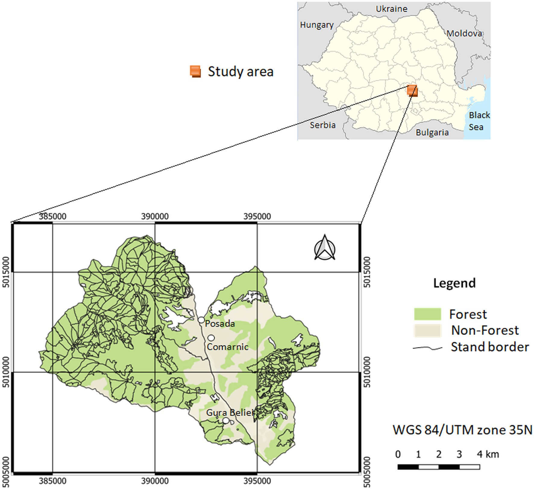
Figure 1. Location of the study area.
Of the entire surface of the studied area, 34.54% was forest, managed by the National Forest Administration, 43.33% was private compact or dispersed forests, and 22.13% was built-up surfaces (buildings, roads, parking lots, etc.), pasture, and hay. The woodlands were dominated by common beech (Fagus sylvatica), Norway spruce (Picea abies), silver fir (Abies alba), European larch (Larix decidua), Scots pine (Pinus sylvestris), and black pine (Pinus nigra), which represented about 89% of the total forest species. The other tree species were sessile oak (Quercus petraea), European hornbeam (Carpinus betulus), grey alder (Alnus incana), black alder (Alnus glutinosa), silver birch (Betula pendula), sycamore maple (Acer pseudoplatanus), European ash (Fraxinus excelsior), aspen (Populus tremula), and willow (Salix caprea).
The proportions of these forest tree species in the overall species composition differed in various parts of the studied area. The main species (beech, spruce, fir, pine, and larch) were generally present in compact stands, but were also found, rarely, in built-up areas. Parts of the stands were pure, while others were mixed, composed of two to three main species. The basal area threshold for distinguishing between pure and mixed stands is 80%; if the basal area exceeds this percentage for a single tree species, then the stand is considered pure, and if it falls below this percentage, the stand is considered mixed. In certain stands, the main species were accompanied, in a small percentage (10–20%), by sycamore maple, ash, sessile oak, and hornbeam. In the southern and middle part of the studied area, built-up areas were present at low altitudes, alternating with pastures and meadows. These areas contained groups of tree species or fruit trees grouped together or growing in rows and along the edges of private properties that were not included in any forest management plans. Here and there in the built-up area, the vegetation occurred as shrubs or was in a different stage of development.
We employed the JavaScript API within the GEE code editor to analyze the data. GEE is a cloud computing platform launched by Google in 2010. It enables users to conduct geospatial analysis and is the most popular platform for processing large geospatial datasets. It includes various built-in algorithms, such as those for classification, allowing for global-scale data analysis and facilitating the development of custom algorithms by researchers. The Earth Engine Data Catalog contains a diverse range of standard Earth science raster datasets that are freely accessible. Additionally, users have the option to upload their own raster or vector data for private use or sharing in scripts. In this study, we used the preprocessed archives of S-1, S-2, and DEM data available on GEE. These preprocessed datasets had already been corrected for atmospheric and topographic effects, which significantly streamlined the data acquisition and preprocessing task, saving us valuable time and effort.
We used 224 S-1 images, gathered in 2021 and 2022. These were ground range detected (GRD) (Level-1) interferometric wide (IW) swath-mode acquisitions that had already been preprocessed, using multi-looking and projection, to the ground range using an Earth ellipsoid model (Copernicus, 2014; Table 1). The spatial resolution of this dataset was measured at 10 m. The S-1 GRD data was processed by thermal noise removal, and radiation and terrain correction, and the 10-m dual bands, VV and VH, of the IW swath mode was selected for further processing to match the resolution of S-2. Because S-1 data were collected from both ascending and descending passes, the VV and VH data were co-registered.
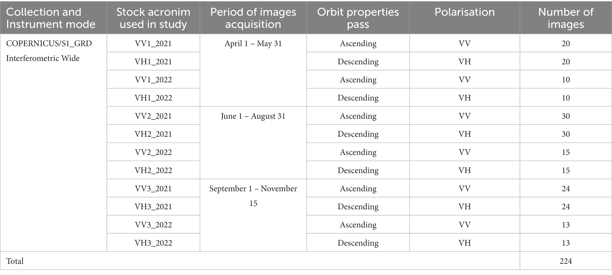
Table 1. Main characteristics of S-1 imagery used in study and the temporal intervals for calculating seasonal composites in 2021 and 2022.
The S-1 images in VV and HV polarization were divided into three temporal intervals for 2021 and 2022. Each temporal interval was specific, from a phenological perspective, to a certain season: April 1 – May 31 (start of the growing season), June 1 – August 31 (peak growing season), and September 1 – November 15 (end of the growing season). In this way, we obtained 12 stock layers (median) that were then compiled individually (Table 1).
We used a set of multispectral data, composed of 15 S-2 surface reflectance images with no cloud cover, acquired in 2021 and 2022 between April 10 and November 26, distributed irregularly over the study periods. The images were downloaded free from Copernicus Data Hub (Table 2). Because tree species analysis depends on phenology, we selected images that had recorded forests in different phenological phases (Hościło and Lewandowska, 2019). In this regard, for both years, we used images acquired at the beginning of spring (when BL species begin to green-up), in the summer (when photosynthetic activity is high), and in the fall (when the leaves begin to color steadily and differently for each tree species). In this way, we chose to include three seasons in the analysis because the signatures exposed in the 15 images during the vegetation season could offer a unique spectral model that could not be obtained by any single image. Unfortunately, we did not find any suitable images for early autumn (September).
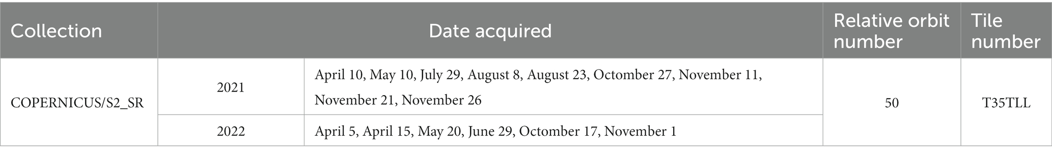
Table 2. Description of the S-2 images used in study.
The downloaded images were orthorectified and atmospherically and topographically corrected at Level-2A (spectral reflectance). For this study, we omitted three bands–coastal (0.43–0.45 μm), water vapor (0.93–0.95 μm), and cirrus bands (1.36–1.39 μm)–because of their sensitivity to atmospheric interference (Stych et al., 2019; Fundisi et al., 2022). The other 10 bands used were red, green, blue, near infrared (NIR), vegetation red edge (VRE), and shortwave infrared (SWIR). They covered a wavelength of 0.41–2.28 μm. The spatial resolution of the S-2 images was 10 m (blue, green, red, and NIR) and 20 m (VRE bands, narrow NIR, SWIR bands). The S-2 bands with the 20-m spatial resolution were resampled to 10 m using the nearest-neighbor resampling method. The resampling was carried out in order to have the same spatial resolution. The images are in WGS84 projection, Zone 35 N.
The topographic variables were derived from the SRTM DEM, which is a free product obtained from interferometric radar. The SRTM provided a near-global DEM between 60°N and 56°S latitude and was realized based on data collected from 11 days in February 2000 by a specially modified radar system onboard the Space Shuttle Endeavour. The SRTM DEM is available globally at 1 arcsecond at about a 30-m spatial resolution. The SRTM DEM was cut on the studied contour and resampled to 10 m (S-2 resolution) using the bilinear resampling method. Based on the SRTM DEM we obtained two topographic variables – slope and aspect – that, together with the elevation, were added to the data stock without any adjustment. In the GEE, the scaling was executed automatically, and all the bands used in different combinations were overlaid correctly.
The high spectral resolution of the S-2 images allowed us to obtain different features connected to the green cover. Based on the literature review, we selected four VIs – the Normalized Difference Vegetation Index (NDVI), Enhanced Vegetation Index (EVI), Green Leaf Index (GLI), and Green Normalized Difference Vegetation Index (GNDVI; Table 3). The NDVI is an indicator of the greenness of the vegetation. High values indicate a rich and healthy vegetation. The EVI was developed because it is more sensitive to changes in areas with high biomass (Bhatnagar et al., 2021). The GLI is intended to measure the quantity of greenery, with positive values representing green leaves and stems. The GNDVI is a modified NDVI, capable of detecting variations in chlorophyll concentration by replacing the red band with the green band (Gitelson et al., 1996).
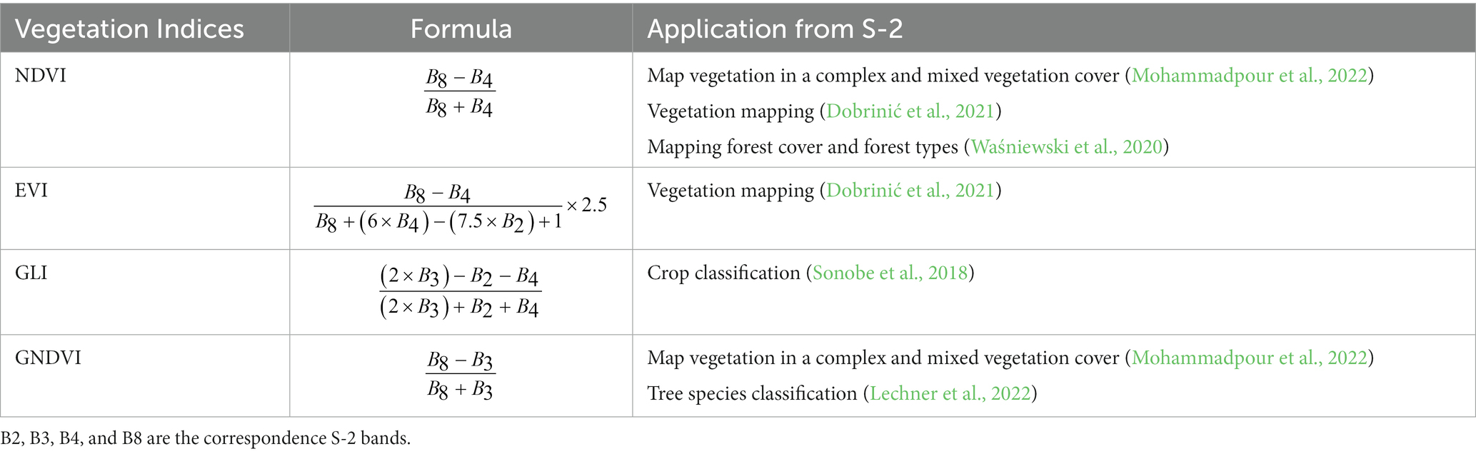
Table 3. Vegetation indices used in the study.
They were selected to offer a comprehensive understanding of various facets of vegetation as these indices offer diverse viewpoints on vegetation health, density, and chlorophyll concentration, inclusively vegetation phenology. By integrating these indices as input variables for classification, the goal was to capture a comprehensive view of vegetation characteristics for the purpose of identifying tree species.
All the images and topographic features used were clipped on the contour of two production units from within the Sinaia Forest District – Forest Management Unit (FMU) I Comarnic and FMU II Posada. The exact geolocations of the boundaries are stored in a GIS database and were provided by the “Marin Drăcea” National Institute for Research and Development in Forestry (NIRDF). These boundaries and stand polygons were converted from Stereografic 1970, the official projection of Romania, in WGS84 projection, Zone 35 N (Greșiță, 2011; Greșiță, 2013). The boundaries of the 2 units (shapefile format) were merged in QGIS and imported into the GEE via Google fusion tables. The obtained contour was used in clipping images and topographic features on the studied area. In addition, all stand polygons were imported in QGIS and the GEE.
The classification process was divided into two levels of forest detail: (i) mapping forest covers; and (ii) classifying tree species. The RF classifier was used for both levels.
The RF is a machine-learning algorithm that uses multiple self-learning decision trees to parameterize models (Hościło and Lewandowska, 2019). In this algorithm, several decision trees are built based on a random subsample of the data used. Each decision tree is produced independently, with no cut, while each node is divided using a defined number of characteristics (Mtry) that were selected randomly (Belgiu and Drăguț, 2016). By increasing the forest to a defined level of usage by using the number of trees (Ntree), the algorithm creates trees that have a higher variance level and a low bias (Breiman, 2001). The final classification decision is taken by obtaining an arithmetical average of the attribution probabilities calculated by all the trees produced (Belgiu and Drăguț, 2016).
The RF classification was carried out using the GEE – a powerful cloud computing platform. The parameterization of the model was performed on 500 single trees in the forest, with the minimum number of samples in a node set to one. Setting Ntree at the 500 level was realized in accordance with the specialist literature, which explains that the errors stabilize before this number of trees are classified (Lawrence et al., 2006). In addition, this value is set as a default value in the R package for RFs (Belgiu and Drăguț, 2016). Mtry parameter was tested from 1 to 9 using a single interval and null value (default in GEE) which means no limits. The last value was considered the best because the overall accuracy was high.
After performing the classification using the RF algorithm, the importance of the variables was estimated through GEE by computing the normalized and raw variable importance. For each classification result, we calculated the importance of the variables.
At the first level, we performed a forest mask by extracting forest areas from all the S-2 images acquired in 2021 and 2022 (Table 2) using the RF classifier. In the non-forested class, we included built-up surfaces (buildings, roads, parking lots, etc.), non-wooded vegetation, agricultural lands (pasture, hay, arable), and water. A ‘No Data’ value was assigned to all pixels not covered by the forest polygons or outside the forested areas mask. The ‘No Data’ pixels were not used for tree species identification. Thus, only pixels with forest and inside the forested areas mask were used.
At the second level, we used different subsets that included various combinations of the two satellite systems, S-1 and S-2, topographic features, and VIs (Table 4). In this stage, we obtained a tree species separation inside the forest mask. All datasets from the second level were classified using the same samples. Figure 2 presents the flowchart of the different classification scenarios.
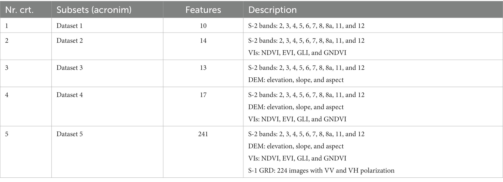
Table 4. Scenarios evaluated using different combinations of S-1, S-2, VIs, and DEM.
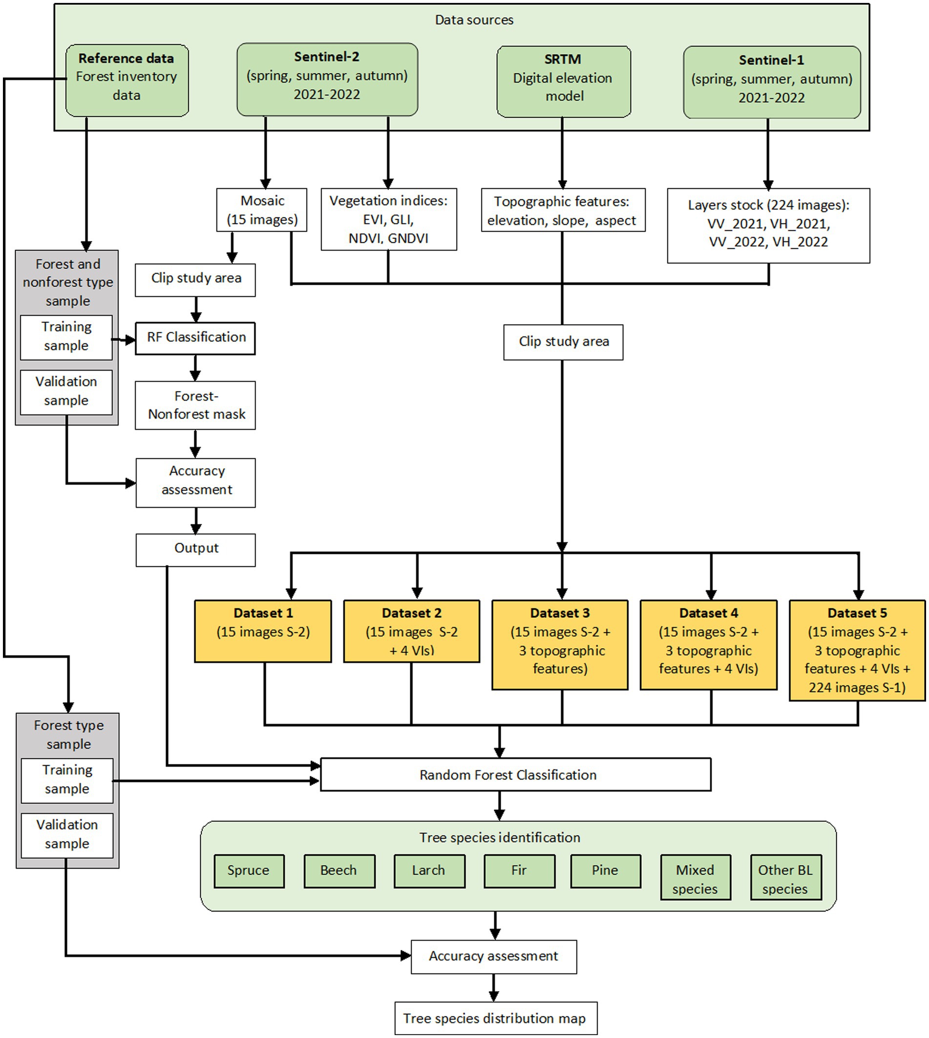
Figure 2. Flowchart of the research.
For this study, we focused on five main stand tree species that collectively represented more than 89% of the total forest of FMU I Comarnic and FMU II Posada–that is, spruce, beech, larch, fir, and pine. Together with these main species, we also identified two groups of species–mixed and other BLs. The mixed species class included both resinous and BL species (including fruit trees) located in urban areas and on private properties, spread on meadows and pastures that were not included in forest management plans. The way in which these patches were grouped was intimate, with the species not being separated based on their components. The other BL species class included species such as oak, maple, sycamore maple, silver birch, European ash, aspen, and willow that were present in small percentages in both the stands and the urban area. They were localized via groups of species. The other BL species were included in forest management plans but located outside those.
Reference data for generating the forest mask were sourced from multiple references, including forest management plan maps, orthophotoplans provided by the National Agency for Cadastre and Land Registration, as well as Google Earth images. Sample selection employed a stratified random sampling approach, where strata were defined by thematic classes. These samples were evenly distributed across the entire study area. For the training and validation datasets, samples were visually chosen from both forested and non-forested polygons, resulting in a total of 193 samples – comprising 84 forested and 109 non-forested areas. These training and validation samples accounted for 7.49% of the forested area and 4.49% of the non-forested area. The average polygon size for forested area was 5.90 ha, while for non-forested areas, it was 0.78 ha. The smaller size on non-forested areas, compared to forested areas, was primarily due to landscape fragmentation.
All training and validation data regarding stand compositions were automatically drawn from the official forestry database of the state forest administration received from the “Marin Drăcea”National Institute for Research and Development in Forestry. This offered detailed information on species composition, stand characteristics (e.g., stand structure, stand density, age, height, medium diameter, and volume), site characteristics (e.g., soil, geology, slope, and orientation), as well as many other types of information (Tereşneu et al., 2016). Forest management plans are updated every 10 years, but major changes, such as stand cutting, plantations and windthrows are recorded annually (Tudoran, 2013). In this way, all the changes that affect stands are recorded in forest management plans at the moment when they are produced. As such, the database is updated and contains all the changes suffered by each stand. The minimum recorded unit is the forest unit, created as a homogenous surface from a silvicultural perspective: to be comprised of a single ecosystem unit or stational unit; the same consistency or differences smaller than 0.2 (on a scale from 0 to 1); the same composition, with difference that do not exceed 20% (on a scale from 0 to 100) for the main species; the average age should not differ more than 20 years; the same type of structure (same age, relatively same age, relativ plurien, plurien); a single productivity category. These criteria were taken into account in the forest inventory in order to demarcate homogeneous stands. Each management unit is demarcated by a polyline that has known coordinates and by marking trees with paint (Tereșneu, 2019; Tudoran and Zotta, 2020). In this study, the stand polygons ranged in size from 0.20 to 44.34 ha (average 5.89 ha) for FMU I Comarnic and from 0.11 to 31.81 ha (average 7.67 ha) for FMU II Posada (Forest Research and Management Institute, 2013a,b).
FMU consists of more forest units. FMU I Comarnic consists of 355 forest units, while FMU II Posada has 111 forest units, all included in the updated database (Forest Research and Management Institute, 2013a). Besides these forest units, approximately 60 forest units belonging to forest owners were also analyzed FMU I Comarnic has a surface of 2091.60 ha (state forest), completed by 907.7 ha (private forests that were retroceded). FMU II Posada has 850.9 ha, completed by retroceded forests (Forest Research and Management Institute, 2013b). The limits of the 2 units are materialized on the field by paint and are represented by natural details (peaks, valleys, waters) or artificial details (roads, railroads etc.). Forest clusters are found inside FMU, on different sizes located within cities.
A forest stand may include, in some cases, five or six different tree species, although the average is usually two, three or four main tree species in a mixture. The tree species composition share in a forest stand is recorded in the forest management plan during the forest inventory. For the present study, we used this share for each management unit. For species with a small share, they were considered together, leading to a distinct class classification (for example, other BL species and mixed species).
Training and validation samples were performed by screen digitization. Each sample was from inside a management unit, with a priority placed on stands with a pure species composition (e.g., with a species share of 100%). Where stands were not pure (i.e., where the share was not 100%), we followed those stands in which the respective species had the largest share.
For tree species that are widespread across the entire analyzed area (such as beech, spruce, and mixed species), the reference sample were evenly distributed throughout the study area. However, for tree species with a more limited distribution (including larch, fir, pine, and other BL species), the reference sample were selectively collected in the specific areas where these tree species are known to occur. In all cases, the selection of reference samples was carried out using a stratified random sampling approach. Table 5 provides detailed information regarding the number of polygons, total area covered, and average polygon size for reference data. Notably, the mixed species class exhibited the smallest average polygon size due to the close proximity of these tree species and their relatively smaller total area. Conversely, the beech class displayed the largest average polygon size, as it typically forms compact stands that extend over a larger geographic area. The choice of remote sensing data used for generating the dataset varied depending on the specific combination (Table 4).
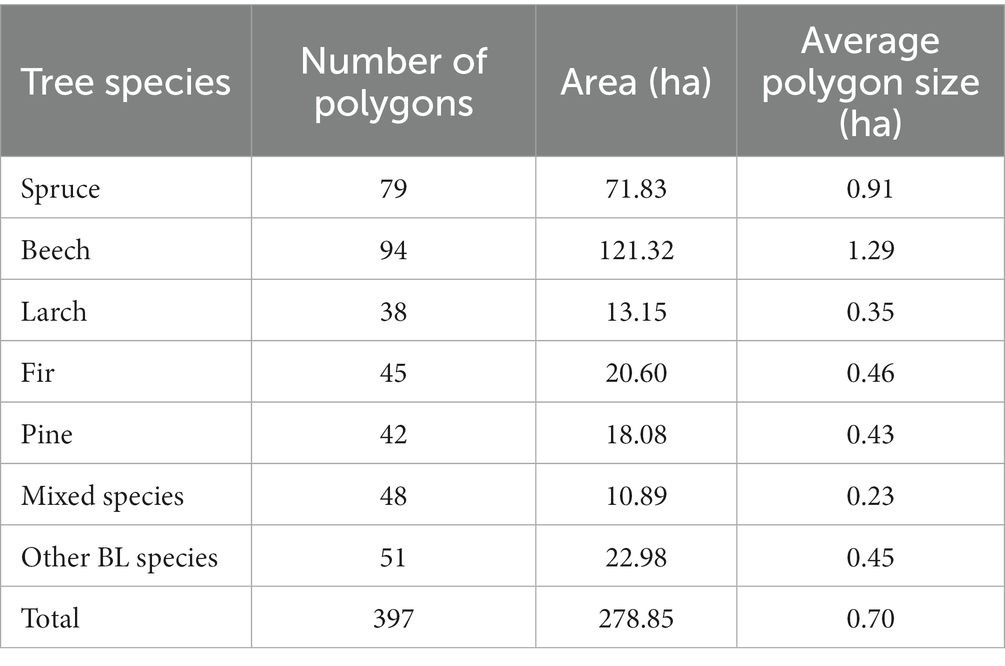
Table 5. Characteristics of reference samples.
In order to validate the data, we used ortophotoplans present in the database from the National Agency for Cadastre and Land Registration, as well as Google Earth images.
The reference samples were randomly divided–80% were used for training and 20% for accuracy assessment purposes. We selected 14,525 pixels for the forest/non-forest map, of which 11,621 pixels were for training and 2,904 for validation. The total number of pixels was 6,971 for the tree species classification, of which 5,577 were for training and 1,395 for validation. To ensure that the tree species proportions are maintained in both datasets, namely the training and validation data, the facilities provided by GEE were used.
An accuracy assessment was performed based on a confusion matrix from which we calculated the overall accuracy indices, in addition to a producer’s accuracy, user’s accuracy, Kappa statistic, and F1 score. Overall accuracy is expressed in percentages and represents the relation between the correctly classified pixels and the total of pixels used for verification. Producer’s accuracy is calculated by dividing the number of correctly classified pixels for a given class by the total number of pixels that belong to that class in the reference dataset.
User’s accuracy is calculated by dividing the number of correctly classified pixels for a given class by the total number of pixels that were classified as that class on the map. The Kappa statistic evaluates how well the classification performs in comparison with the random attribution of values. The F1 score is the harmonic mean of precision and recall.
Establishing samples for accuracy assessment was realized through stratified proportional random sampling. Through this method, the total number of pixels was distributed in each class, in report with the surface of the tree species from the analyzed surface. The strata were represented by the tree species present in the classified images. Within each strata, validation data were sampled using a random method. The sampling units were individual pixels. The accuracy assessment was carried out individually for each classification result.
The result of the forest/non-forest classification derived from all the multitemporal S-2 images using the RF approach showed a high level of agreement with the forest status on the ground. The overall accuracy of the forest/non-forest map was 99.48%, with a Kappa coefficient of 98.01%. The producer’s accuracy for the forest was 99.71, and 98.20% for the non-forest. The user’s accuracy for the forest was 99.67, and 98.42% for the non-forest (Table 6). Because we obtained a high accuracy, we used the output of the RF classification derived from combination with the S-2 images to calculate the forest area for the study area and the forest mask. Under these conditions, the surface covered by forest was 6,634 ha, representing 77.87% of the studied surface. Of this forest surface, 2,942 ha (44.35%) were managed by the state, while 3,692 ha (55.65%) represented private property.
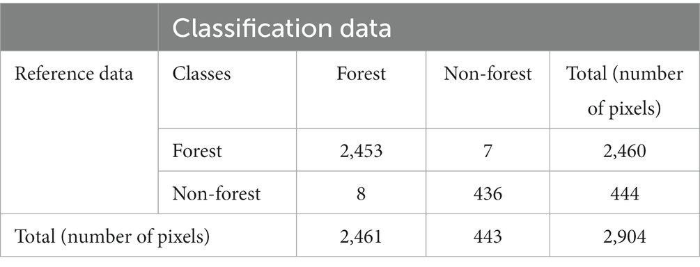
Table 6. Error matrix for forest and non-forest classification.
The results regarding the overall accuracy of the tree species classification, based on the five sets of data, are presented in Figure 3. A very close overall accuracy was obtained for three of these combinations (Datasets 3–5). The best result was obtained for Dataset 5, with an overall accuracy of 89.68%, followed by Dataset 3, with 89.51%, and Dataset 4, with 89.36% (Figure 3A). The lowest result was obtained by Dataset 1, which included only S-2 satellite images, and had an overall accuracy of 76.74%.
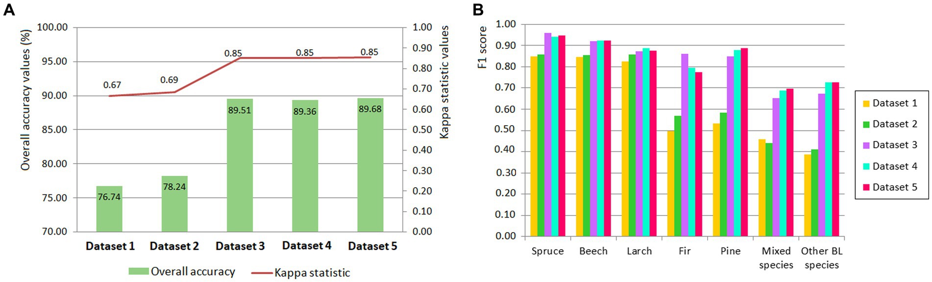
Figure 3. Overall accuracies and Kappa statistics for the five datasets used in tree species identification (A) and F1 score (B).
Evaluation of the classification performance for Dataset 5 among the individual tree species showed good results for spruce (93.82%), larch (93.44%), and fir (92.96%). These three species corresponded quite well to the forest stands. For spruce, 16 pixels were confused with beech, while for larch, 7 pixels were confused with beech, for fir, 15 pixels were confused with beech and 11 pixels with spruce (Table 7). Slightly weaker results were obtained for mixed species (86.96%) and other BL species (87.06%). For mixed species, 9 pixels were classified as beech and 33 pixels for other BL species.
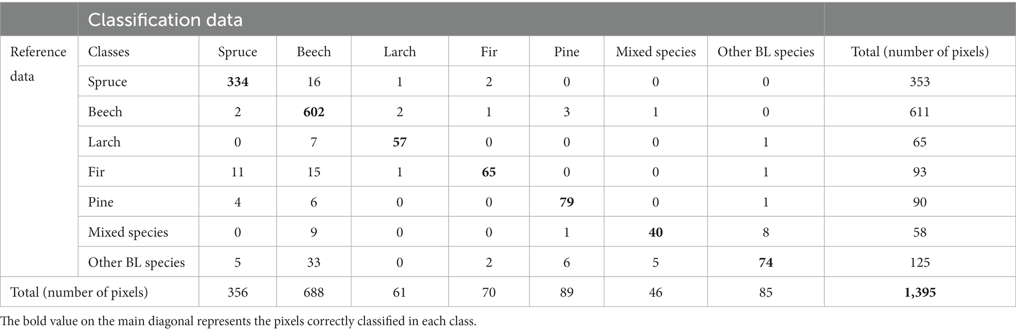
Table 7. Confusion matrixs for RF classification of seven tree species inside of forest mask using dataset 5.
The results obtained after calculating the F1 score for each tree species show that they are close for the 3–5 Dataset. Spruce is best discriminated in Dataset 3, with an F1 score equal to 0.96, while beech is best discriminated in all three data sets, with an F1 score of 0.93 (Figure 3B). As for larch, the best discrimination is in Dataset 4, as well as in the other four datasets, while F1 varies from 0.83 (Dataset 1) to 0.89 (Dataset 4). Fir is identified better in Dataset 5, with an F1 score of 0.89. Mixed species (F1 = 0.70) and other BL species (F1 = 0.73) are the two group of species with the less confidence (Figure 3B).
Based on the evaluation of the overall accuracy of the classification, we created the final map with tree species from the best combination–Dataset 5 (Figure 4).
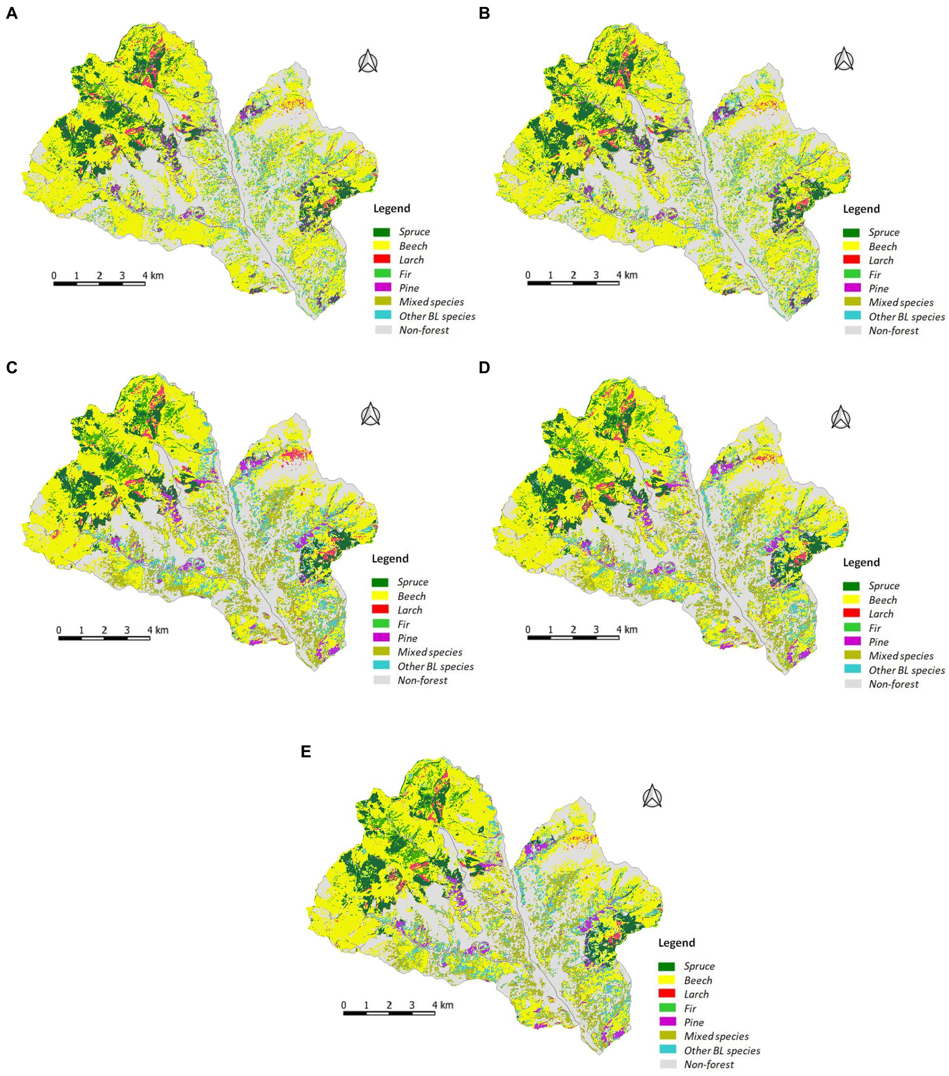
Figure 4. Tree species identification maps generated using RF classification for: (A) Dataset 1; (B) Dataset 2; (C) Dataset 3; (D) Dataset 4; (E) Dataset 5.
The importance of the variables used in the classification of the tree species is presented in Figure 5. These were prioritized based on importance level. The DEM contributed the most toward classifying the datasets (Datasets 3–5). Together with elevation, aspect and slope proved to be the most important variables. They also determined an evident increase in the overall accuracy. With regard to the S-2 spectral bands, B12 and B11 (SWIR) were the most important contributors in separating the tree species in all the datasets. Band 8 (NIR) obtained the lowest scores in the tree datasets. The inclusion of VIs in three of the datasets, combined with the S-2 bands, DEM, and S-1 bands, did not produce a high rate when compared with DEM, aspect, and slope. The GLI and EVI indices made the highest contribution of all the VIs, while the NDVI contributed the least. Even though we used many S-1 images, their contribution to classifying the tree species was minimal.
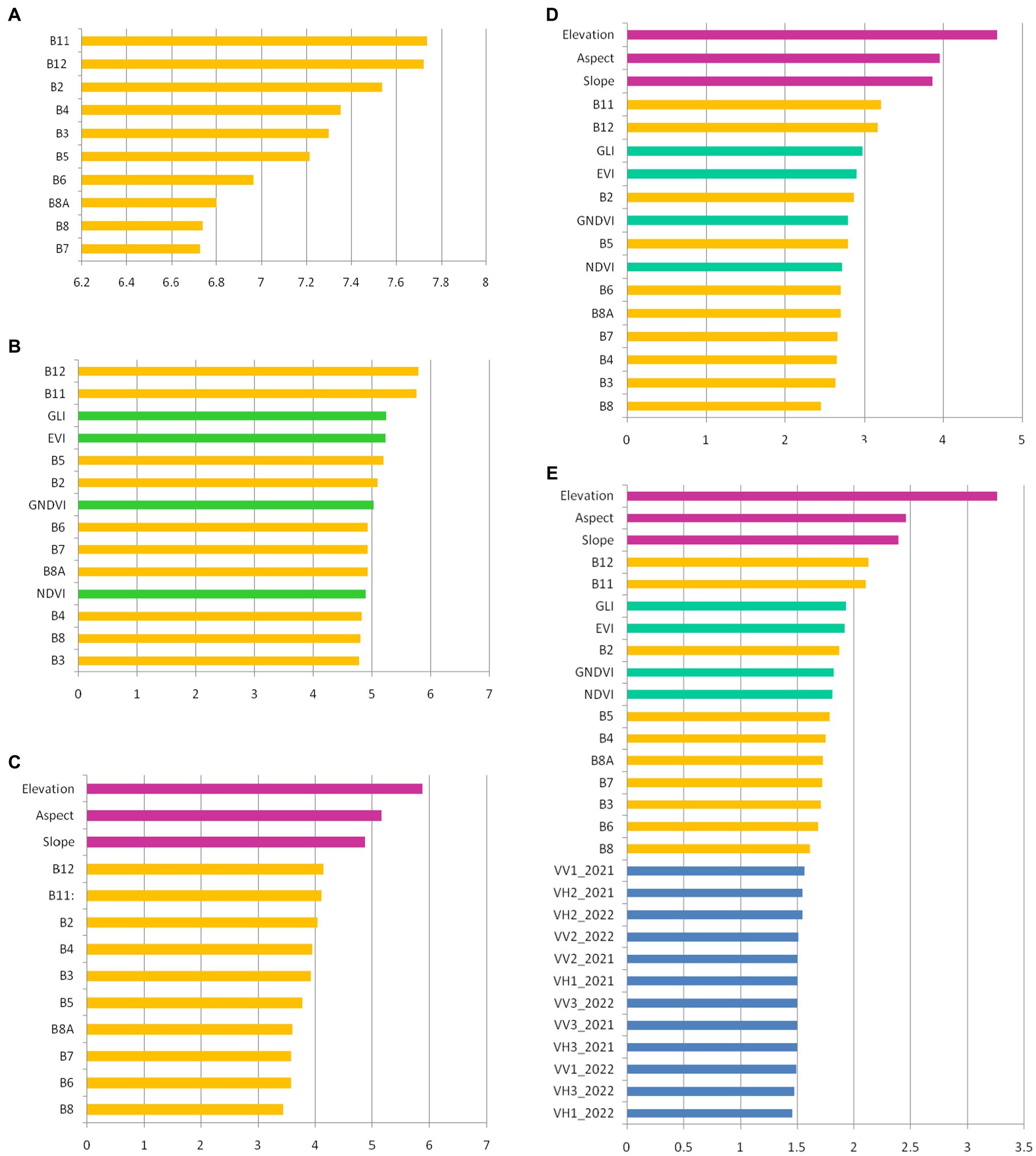
Figure 5. The variable importance for tree species classification: (A) Dataset 1 (S-2 images); (B) Dataset 2 (S-2 images and VIs); (C) Dataset 3 (S-2 images and topographic features); (D) Dataset 4 (S-2 images, VIs and topographic features); (E) Dataset 5 (S-2 images, VIs, topographic features, and S-1 images). The colors are as follows: orange – spectral bands of S-2 images; green – VIs; magenta – topographic features; blue – layer stacks of S-1 images (according Table 1).
We mapped tree species using different combinations of dense S-1 and S-2 time-series images, VIs derived from optical S-2 bands, and topographic features derived from a DEM. The S-1 and S-2 images were taken in two growing seasons (2021 and 2022), allowing us to obtain detailed information about the spectral-temporal patterns of the studied species. This study was performed on an area with a heterogeneous distribution of vegetation, including both dense forests on massifs and tree species grouped in patches of different sizes that alternated with built-up areas, pasture, and hay.
Combining the 15 S-2 images taken from the two vegetation seasons led to an overall accuracy of 76.74%. In this combination, SWIR bands (B11 and B12) had the highest importance, while B8 and B7 had the lowest (Figure 5A). The low importance of Bands B8 and B7 can be explained by the fact that many of the S-2 images were acquired during spring and autumn, not during summer, when the photosynthetic activity is strong and the reflectance in NIR is also high. However, the sun’s elevation angle is low during early spring and late autumn–an effect that could lead to a decrease in the classification’s accuracy (Hościło and Lewandowska, 2019).
The results regarding the overall accuracy of the tree species classification, based on the five sets of data, are presented in Figure 3. A very close overall accuracy was obtained for three of these combinations (Datasets 3–5). The best result was obtained for Dataset 5, with an overall accuracy of 89.68%, followed by Dataset 3, with 89.51%, and Dataset 4, with 89.36%. The weakest result was obtained by Dataset 1, which included only S-2 satellite images, and had an overall accuracy of 76.74%.
By including the VIs in the classification, together with the S-2 images (Dataset 2), the overall accuracy reached 78.24%, increasing by only 1.5%. This result is similar to that of Mohammadpour et al. (2022), who mentioned that a slight accuracy increase was obtained by combining four VIs with S-2 images, compared with only using spectral bands. Another study (Spracklen and Spracklen, 2019) showed that adding six VIs to identifying European old-growth forests led to a worse performance from using them in combinations instead of the S-2 bands, resulting in the overall accuracy being reduced by 0.3%. On examining the relative importance of the variables, we can see that, in this case as well, Bands B11 and B12 were in first place, followed by the GLI and EVI. The GNDVI and NDVI contributed the least among all the indices. The low importance of the NDVI in classifying tree species has also been signaled by other studies (Pouteau et al., 2018; Silveira et al., 2018).
Choosing VIs in emphasising the vegetation phenology is important. EVI and GLI proved to be the most suitable in identifying phenological changes as they are more strongly correlated with the crown’s foliage. The high separability on which it is based derives from spectral bands with blue, green and near infrared reflectance. EVI emphasises better the phenology, compared with NDVI in surfaces with both dense and sparse vegetation (Tian et al., 2021). Furthermore, Bolton et al. (2020) have shown the high two-band EVI (EVI2) capacity in emphasising the phenology of ecosystems with a strong seasonality, namely deciduous trees species, and less for those with evergreen species. The share brought by VIs in identifying resinous species was marginal because the crown is green all year long. NDVI-derived phenology is uncertain for surfaces covered with resinous trees where the seasonal amplitudes are small (Tian et al., 2021).
An important leap in overall accuracy came from adding topographic features to the S-2 images (Dataset 3), when 89.51% was obtained. The results obtained in this study are in line with those from other studies. Hościło and Lewandowska (2019) classified eight tree species with an accuracy of 75.6% using only S-2 data. By adding a DEM, slope, and aspect, an accuracy of 81.7% was reached by classifying all species together, with 89.5% achieved for a stratified classification. In Liu et al. (2018), the importance of slope derived from a DEM was demonstrated in the classification of four common species and four mixed forests located in China. The importance of a DEM in classifying species and obtaining high accuracy has also been reported in other studies (Waśniewski et al., 2020; Dobrinić et al., 2021). In the present study, we proved that the DEM contributed the most, followed by aspect and slope (Figure 5C). This means that the presence of species in the studied area was highly dependent on elevation.
The S-1 images, VIs, and topographic features combination (Dataset 4) decreased the accuracy by 0.15%, compared with the S-2 plus topographic features combination (Dataset 3). These results are similar to those from other studies that showed that adding the NDVI led to a decrease in accuracy of 8% (Mohammadpour et al., 2022). Other studies have shown that adding the NDVI to a combination of S-2 images and a DEM leads to a decrease in accuracy of 3% (Waśniewski et al., 2020). In the present case, the decrease in overall accuracy can be associated with a decrease in user accuracy for spruce, beech, larch, and other BL species (Figure 3).
In the S-1, S-2, VIs, and topographic features combination (Dataset 5), we obtained an overall accuracy of 89.69%. Compared with the overall accuracy resulting from combining S-2 images with topographic features (Dataset 2), the overall accuracy increased by only 0.17%, and by 0.32% compared with the S-2, VIs, and topographic features combination (Dataset 4). By analyzing the contributions of the variables, we can see that the importance of the S-1 images was minimal, even though their number was high when compared with the other variables (Figure 5E).
The results obtained from this study are very close to the ones obtained by Lechner et al. (2022), where, by adding 250 S-1 images for 14 S-2 images taken from a vegetation season, the accuracy was only 0.5%. Liu et al. (2018) demonstrated that adding backscattering features from VV images of S-1 to the combination of S-2, DEM, and Landsat 8 provided only a modest 2.65% improvement in classifying forest types, compared to the same combination without S-1. Furthermore, the additional of VV and HV features from S-1 to the combination with S-2, DEM, and Landsat 8 actually resulted in a 1.32% decrease in accuracy when compared to using the combination of S-2, DEM, and Landsat 8 alone. This indicates that VV polarization images are more effective in discriminating forest types than VH polarization data. Additionally, the fusion of S-2 with S-1 yielded only a marginal 1.5% increase in overall accuracy for forest mapping (Hirschmugl et al., 2018). In another study, it was found that using S-1 images in combination with S-2 images to distinguish between plantations and natural forests led to a slight decrease in accuracy, from 92.5% achieved using S-2 alone to 92.3% for S-1 and S-2 combination (Spracklen and Spracklen, 2021). Therefore, integrating S-1 data with S-2 did not significantly enhance accuracy and, in some cases, even resulted in a slight reduction of 0.2%. Consequently, the addition of S-1 images only marginally improves accuracy or may potentially lead to a decrease in accuracy.
Achieving only a marginal increase in accuracy through the combination of S-1 with S-2 images can be attributed to several factors. For instance, S-1 images capture data that reflect surface properties such as its structure and roughness. Lechner et al. (2022) found that within the conifer group, when separated using S-1 images, achieving satisfactory accuracy may be related to the more pronounced roughness of conifer crowns compared to those of deciduous trees. Furthermore, in comparison to the multispectral data of S-2 images, S-1 data do not provide so much detailed information about the biometric and spectral characteristics of vegetation. Additionally, S-1 images can be influenced by factors such as soil moisture and vegetation density, which can lead to variations in captured signals and more complex data interpretation. In the study conducted by Xi et al. (2023), it is shown that the contribution of S-1 images to forest diversity estimation was found to be rather limited, possibly due to the relatively short frequency of the C-band, making it less sensitive to characterizing dense forest canopies. Moreover, C-band radar waves are strongly attenuated by tree canopies, causing intensities to be similar for plant types with subtle structural differences (Ienco et al., 2019; Slagter et al., 2020). Furthermore, physiologically similar tree species cannot be differentiated using S-1 data (Heckel et al., 2020). In such cases, the spectral response of tree species recorded in S-2 images is more valuable in distinguishing between them, with less contribution from S-1 images.
The forest of the study area was divided into seven classes. Sampling data was collected by visually interpreting images and ortophotoplans, and by comparing these with Google Earth images. The sampling size was approximately 3.4% for training and 0.8% for testing from the total surface (Table 8). Dividing them in training (80%) and validation (20%) samples was made randomly, according to the code written in GEE. According to the specialty literature, the sample size was indicated to be between 0.2 and 3.0% of the total data (Blatchford et al., 2021). Therefore, the samples were sufficient for training classifiers and were relatively uniformly spread across the entire studied area.
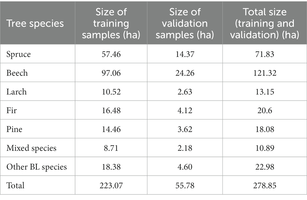
Table 8. The size of training and validation samples for each of the tree species.
For Dataset 1, by using only the S-2 multitemporal images, the tree species that had low user accuracy values were fir (61.54%), pine (60.00%), mixed species (62.50%), and other BL species (52.38%). By using only the S-2 images, Immitzer et al. (2016) obtained the same user accuracy for pine, while spruce reached a user’s accuracy of 77%, fir 71%, and larch 64%. The discrimination capacity for these species substantially increased after adding elevation, slope, and aspect as variables to the S-2 images (Dataset 3). By adding topographic features, the most substantial increases in accuracy for the tree species were (Figure 6) 26.30% (fir), 22.29% (pine), 11.31 (mixed species), and 33.70% (other BL species). Smaller accuracy increases were observed for other tree species–spruce (11.54%), beech (9.86%), and larch (12.00%).
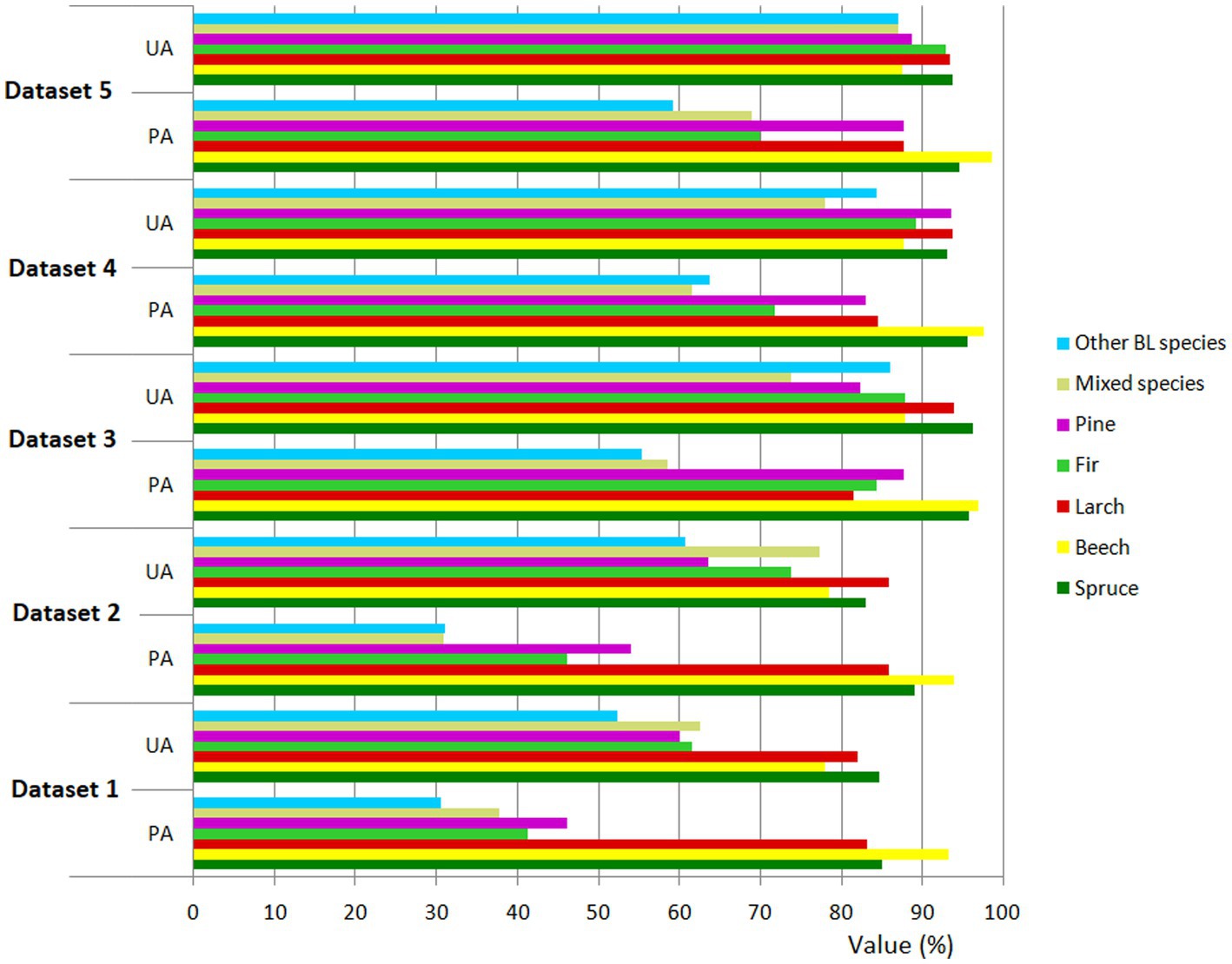
Figure 6. Class level accuracy assessment (producer’s accuracy – PA and user’s accuracy - UA) for all tree species and datasets mapped by RF classification.
However, using an increasing number of variables in the classification did not necessarily lead to greater accuracy for all tree species (Figure 6). This was particularly notable for spruce, larch, and other BL species when, by adding VIs in combination with S-2 images and topographic features (Dataset 3), the user accuracy decreased by 3.14, 0.19, and 1.70%, respectively (Figure 6).
Looking globally, the overall accuracy increase from 76.74% (Dataset 1) to 89.68% (Dataset 5) was resulted from increasing the discrimination capacity for fir, pine, mixed species, and other BL species. The user accuracy increases were 31.32% (fir), 28.76% (pine), 24.42% (mixed species), and 34.68% (other BL species). As has already been shown, these increases were not linear (Figure 6). In the case of spruce, by adding new bands to the classification, apart from the S-2 bands, the increase in user accuracy was 9.18%, with 9.56% for beech, and 11.5% for larch – considerably lower than for the other species. For example, the accuracy increase was 9.53% for spruce, 5.3% for beech, and 4.59% for larch. Important increases were recorded for fir (28.65%), pine (41.63%), mixed species (31.32%), and other BL species (28.64%).
At the conifer/BL level, the results showed that coniferous species were classified better than BLs. In terms of the separation of coniferous tree species, the best user’s accuracy was obtained for spruce (93.82%), larch (93.44%), fir (92.96%), and pine (88.86%). Stoffels et al. (2015) obtained a user’s accuracy of 91.6% for spruce, which is close to the value from the present study. Hościło and Lewandowska (2019) applied the stratified approach to the S-2 multitemporal images and topographic features, obtaining separation accuracy of 85% for spruce, 84.1% for pine, and almost 80% for larch and fir. Lower accuracy was obtained by Immitzer et al. (2012) for spruce (80.4%), pine (85.1%), larch (70.4%), and fir (82.3%) using very high spatial resolution 8-band Worldview-2 satellite data. In the case of the BLs, the highest user’s accuracy was obtained by beech (87.50%), followed by other BL species, with a user’s accuracy of 87.06%, and mixed species, with 86.96%. Immitzer et al. (2016), using S-2 images, recorded a user’s accuracy of 73.8% for beech and 51.4% for BL species. Hościło and Lewandowska (2019) used S-2 images and topographic features, achieving a beech user’s accuracy of 92.3%.
According to the classification for which the highest overall accuracy was obtained (Dataset 5), the most widespread species in the study area were beech (56.21%), mixed species (13.30%), and spruce (10.27%). The order of decrease in the occupied surface was BLs (9.15%), fir (5.47%), pine (3.36%), and larch (2.24%; Figure 7). The obtained surfaces could not be verified because we lacked forest evidence from outside the forest management plan and for the private areas.
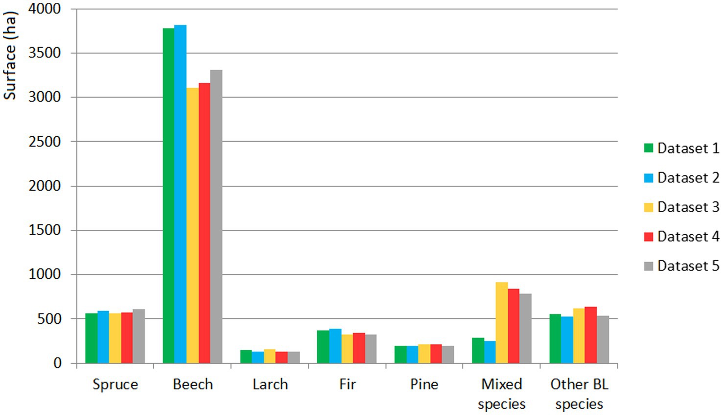
Figure 7. The areas occupied by tree species according to of the RF classification for the five datasets.
Mapping tree species using multitemporal data S-2 are generally based on leaf seasonality, and the main phenophases such as budburst, leaf unfolding, autumn colouring, and abscission. In the case of deciduous trees, seasonal variations in the efficiency of the photosynthetic activity are strongly emphasised during autumn, through the senescence process which is strongly connected with leaf colouring. The importance of the six S-2 images from autumn (October and November), when the leaf colouring process appeared, is crucial in separating tree species, especially deciduous trees. However, the very similar spectral signatures for beech, hornbeam, sessile oak, grey alder, sycamore maple, and European ash have led to a lower accuracy of mixed species and other BL species. This phenomenon was also emphasised by other studies (Hill et al., 2010; Pasquarella et al., 2018; Grabska et al., 2019). Furthermore, the phenological differences were difficult to capture for species characterised by very close phenological phases (for example, between beech and hornbeam). This situation was also reported by other studies (Schieber et al., 2009). The five images used in the study and acquired during spring (April and May), are depicting tree species phenology through different moments of leaf green colouring. The species located at lower altitudes have greened faster than the ones located at higher altitudes. Both cases depend on the temperature. For example, beech foliation depended on temperatures from March, at lower altitudes and on April temperatures as the altitude increases.
The photosynthetic activity of resinous species is rather hard to quantify based on satellite images, but seasonal changes can be quantified in the visible spectra (Gamon et al., 2016). Generally speaking, the spectral behaviour of spruce and fir is similar, but differs significantly from pine, indicating a difference between the phenology of pines and other resinous species. Larch, the only resinous species from the present study, has shown a spectral signature closed to deciduous trees that increased during autumn in the visible and SWIR bands. All the other resinous did not have obvious phenological phases, but needle appearance during spring can be an indicator of growth start that can be seen on spring images.
The classification errors could have different causes. Using samples based on data from forest management plans could be one of them. Even though stand composition is established through forest inventory, disparities can occur. The small training dataset could also be the reason for some of the confusion in classifying the tree species. To some degree, this failed to provide a coherent spectral reflectance. This was the case for species such as larch and pine that were present in small percentages (10–20%) in the composition of some stands. Another cause could be the inclusion of pixels that represented other species in the samples. This was found to be the case for beech and hornbeam mixtures, oak, sycamore maple, ash, aspen, silver birch, grey alder, and black alder. These were disseminated in the stands and, because of their similar spectral behaviors, confusions appeared where the accuracy was lower for mixed and other BL species. Furthermore, obtaining samples for the same species in stands of different ages likely led to selecting some different spectral signatures. For example, beech had a very high intensity signature in some samples and a dark signature in others, leading to its classification as resinous.
Global change and tree species identification are interconnected topics that play a crucial role in understanding and addressing the challenges facing our planet’s forests. Tree forest identification through satellite imagery and remote sensing techniques allows for continuous monitoring of forest an global scale. It is essential for monitoring changes in forest cover, understending the distribution of tree species, and assessing the health and resilience of forests. Global change factors, such as rising temperatures, altered precipitation patterns, and increase frequency of extreme weather events, influence the growth, reproduction, and survial of tree species. Consequently, certain trees my encounter difficulties in adapting to this conditions, leading to shifts in forest composition and distribution. All the forests in the analyzed area are categorized as forests with special protection functions. Understanding the composition and distribution of tree species in such an area is crucial for ensuring the forest’s functions as designated in the forest management plan.
In the context of global change, tree species identification is crucial for identifying areas that have undergone deforestation or degradation. By knowing the original species composition, efforts to restore this forests can focus on reintroducing the right tree species and promoting ecosystem resilience. In the studied area, these forests are categorized within the forest management plan as tree stands situated on rocky outcrops, scree slope, lands with deep erosion, or on terrain with a slope exceeding 35 degrees. In this way, strategies for planting and regenerating forests can be developed in accordance with the requirements of the species (Abrudan, 2006), thus preventing the negative effects of planting in unsuitable areas, such as fungal and insect attacks.
Different tree species have varying abilities to sequester carbon dioxide from the atmosphere, making tree species identification crucial for estimating carbon stocks in forests. In this sense, forests play a critical role in mitigating climate change by acting as carbon sinks, capturing and storing significant amounts of carbon (Goetz et al., 2009). Additionally, in the case of urban forests and rapid urbanization, it is essential to investigate the role of these forests in maintaining air quality, biodiversity, and the quality of life in cites, and to develop policies for managing these changing ecosystems. This applies to the forests in the lower and middle parts of the studied area, encompassing 257.9 ha, which are designated in the forest management plan as forests with recreational and social significance.
Tree species identification is vital for conservation efforts. By knowing the tree species present in a forest, conservationists can develop targeted strategies to protect and restore specific habitats, especially those of threatened or endemic species. Certainly, within the studied area, 442.09 ha of FMU II Posada are encompassed by the Natura 2000 site ROSCI0013 Bucegi. The encountered Romanian habitat types consist of Southeastern Carpathian forests featuring spruce, beech, and fir with Pulmonaria rubra, as well as Southeastern Carpathian beech forests with Symphytum cordatum, both of which require conservation efforts. Furthermore, an additional 285.85 ha of forest serve as buffer zones for the reserves within the Bucegi Natural Park. Additionally, 94.73 ha of forests are designated as reserves for seed production and the preservation of the forest gene pool. It also aids in planning sustainable forest management practices that consider the needs of different species. By understanding changes in tree species distribution, forest managers and policymakers can adapt their strategies to address emerging challenges posed by global change. In the analyzed area, several essential activities are required to support natural regeneration, maintain an optimal mix of tree species, control invasive tree species, and manage mature forest to preserve a high level of biodiversity.
Additionally, identifying tree species on satellite images helps to identity fire-prone areas and monitor illegal logging activities. By monitoring tree species, strategies for fire risk management and effective firefighting can be developed (Jaiswal et al., 2002). Moreover, by identifying tree species through remote sensing data, the impact of human activities on forests, such as excessive logging, agricultural expansion, and urban development, can be analysed. In this way, appropriate measures for protection and ecological restoration can be taken. The analysed area also serves as a tourist destination, featuring human settlements in its central region. This necessitates vigilant monitoring of human activities within the forested areas and urban development.
Overall, tree species identification using satellite images is an essential tool for understending the impact of global change on forests and developing effective strategies for conservation, adaptation, and sustainable management. It helps us to make informed decisions to protect and preserve our valuable forest ecosystems in the face of ongoing environmental challenges.
In this study, the performance of S-1 and S-2 images, VIs, and topographic features in various combinations were investigated as tools for tree species mapping. Seven tree species–four coniferous and three deciduous–located in a complex mountain area characterized by compact forests and forests fragmented by private property, were classified using the RF algorithm. The accuracy of the classification was compared for five different combinations (datasets) of input variables. This showed the importance of phenology, together with topographic features (elevation, aspect, and slope), in improving the performance of the RF classifier in the classification of tree species. Using topographic features also guaranteed that a sample belonged to a particular tree species based on its precise altitudinal distribution.
Because phenology varies with species, it is important to select S-2 images that represent the phenological cycle of the studied tree species when mapping tree species. Seasonal S-2 composites have advantages over monotemporal classifications, but preference should be given to a combination of S-2 images and topographic features. Bands B11, B12, and B2 contributed the most among the S-2 bands used in this study, allowing the capturing of differences among the species during the growing season, and analyzing their temporal patterns. The S-2 satellite has numerous advantages, such as high temporal resolution and being able to provide data more frequently than other medium-resolution sensors.
Combining VIs with the S-2 images did not bring a substantial accuracy advantage, but GLI and EVI made the largest contribution. By bringing together S-1 images combined with S-2 images, VIs, and topographic features, the effect was only marginal, while the accuracy was very low. However, the results have indicated that introducing S-1 images into the classification caused a shift in the contributing features. As such, they had a more important role in classifying groups of species from BL species and mixed species. This approach has allowed us to establish that the lowest accuracy was obtained in the hill area, where there was less forest cover and more forest fragmented by private property, and around the margins of stands that contained different species. The highest accuracy was obtained from compact, pure, and homogenous stands from mountain areas, where the degree of forest coverage was very high.
The original contributions presented in the study are included in the article, further inquiries can be directed to the corresponding author.
IV supervised and coordinated the research and wrote the manuscript. LD, CV, RGP, and CC helped with the study conception and design, performed material preparation, data collection and analysis, read and commented on previous versions of the manuscript. CLC, CIG, SC, and IG participated in data validation. All authors contributed to the article and approved the submitted version.
The authors are thankful to the European Space Agency (ESA) for providing Sentinel-1 and Sentinel-2 images for free of charge. Also, authors thanks to National Institute for Research and Development in Forestry “Marin Drăcea” for provided the references data.
The authors declare that the research was conducted in the absence of any commercial or financial relationships that could be construed as a potential conflict of interest.
All claims expressed in this article are solely those of the authors and do not necessarily represent those of their affiliated organizations, or those of the publisher, the editors and the reviewers. Any product that may be evaluated in this article, or claim that may be made by its manufacturer, is not guaranteed or endorsed by the publisher.
Abrudan, I. V. (2006). Afforestation (in Romanian). Brașov: Transilvania University Publishing House.
Ballanti, L., Blesius, L., Hinnes, E., and Kruse, B. (2016). Tree species classification using hyperspectral imagery: a comparison of two classifiers. Remote Sens. 8, 445–463. doi: 10.3390/rs8060445
Belgiu, M., and Drăguț, L. (2016). Random forest in remote sensing: a review of applications and future directions. ISPRS J. Photogramm. Remote Sens. 114, 24–31. doi: 10.1016/j.isprsjprs.2016.01.011
Bhatnagar, S., Gill, L., Regan, S., Waldren, S., and Ghosh, B. (2021). A nested drone-satellite approach to monitoring the ecological conditions of wetlands. ISPRSJ. Photogramm. Remote Sens. 174, 151–165. doi: 10.1016/j.isprsjprs.2021.01.012
Blatchford, M. L., Mannaerts, C. M., and Zeng, Y. (2021). Determining representative sample size for validation of continuous, large continental remote sensing data. Int. J. Appl. Earth Obs. Geoinf. 94:102235. doi: 10.1016/j.jag.2020.102235
Bolton, D. K., Gray, J. M., Melaas, E. K., Moon, M., Eklundh, L., and Friedl, M. A. (2020). Continental-scale land surface phenology from harmonized Landsat 8 and Sentinel-2 imagery. Remote Sens. Environ. 240:111685. doi: 10.1016/j.rse.2020.111685
Clark, M., Roberts, D., and Clark, D. (2005). Hyperspectral discrimination of tropical rain forest tree species at leaf to crown scales. Remote Sens. Environ. 96, 375–398. doi: 10.1016/j.rse.2005.03.009
Copernicus (2014). Sentinel-1 Data Access and Products European Space Agency. Available at: https://dataspace.copernicus.eu/explore-data/data-collections/sentinel-data/sentinel-1 (Accessed March 18, 2023).
Dian, Y., Li, Z., and Pang, Y. (2014). Spectral and texture features combined for forest tree species classification with airborne hyperspectral imagery. Indian Soc Remote Sens 43, 101–107. doi: 10.1007/s12524-014-0392-6
Dmitriev, E. (2014). Classification of the forest cover of Tver oblast using hyperspectral airborne images. Izv. Atmos. Ocean. Phys. 50, 929–942. doi: 10.1134/S0001433814090072
Dobrinić, D., Gašparović, M., and Medak, D. (2021). Sentinel-1 and 2time-series for vegetation mappingusing random forest classification: a case study of northern Croatia. Remote Sens. 13:2321. doi: 10.3390/rs13122321
Dorren, L. K. A., Maier, B., and Seijmonsbergen, A. C. (2003). Improved landsat-based forest mapping in steep mountainous terrain using object-based classification. For. Ecol. Manag. 183, 31–46. doi: 10.1016/S0378-1127(03)00113-0
Dostálová, A., Lang, M., Ivanovs, J., Waser, L. T., and Wagner, W. (2021). European wide forest classification based on Sentinel-1 data. Remote Sens. 13:337. doi: 10.3390/rs13030337
Farreira, M. P., Zortea, M., Zanotta, D. C., Shimabukuro, Y. E., and de Souza Filho, C. R. (2016). Mapping tree species in tropical seasonal semi-deciduous forests with hyperspectral and multispectral data. Remote Sens. Environ. 179, 66–78. doi: 10.1016/j.rse.2016.03.021
Fassnacht, F. E., Latifi, H., Stereńczak, K., Modzelewska, A., Lefsky, M., Waser, L. T., et al. (2016). Review of studies on tree species classification from remotely sensed data. Remote Sens. Environ. 186, 64–87. doi: 10.1016/j.rse.2016.08.013
Forest Research and Management Institute (2013a). Forest Management Plan of Forest Management Unit I Comarnic (in Romanian). Brașov, Romania: Marin Dracea, ICAS. 156 p.
Forest Research and Management Institute (2013b). Forest Management Plan of Forest Management Unit II Posada (in Romanian). Brașov, Romania: Marin Dracea, ICAS. 148 p.
Fundisi, E., Tesfamichael, S. G., and Ahmed, F. (2022). A combination of Sentinel-1 RADAR and Sentinel-2 multispectral data improves classification of morphologically similar savanna woody plants. Eur. J. Remote Sens. 55, 372–387. doi: 10.1080/22797254.2022.2083984
Gamon, J. A., Huemmrich, K. F., Wong, C. Y. S., Ensminger, I., Garrity, S., Hollinger, D. Y., et al. (2016). A remotely sensed pigment index reveals photosynthetic phenology in evergreen conifers. Proc. Natl. Acad. Sci. 113, 13087–13092. doi: 10.1073/pnas.1606162113
Gitelson, A. A., Kaufman, Y. J., and Merzlyac, M. N. (1996). Use of a green channel in remote sensing of global vegetation from EOS-MODIS. Remote Sens Environ. 58, 289–298. doi: 10.1016/S0034-4257(96)00072-7
Goetz, S. J., Baccini, A., Laporte, N. T., Johns, T., Walker, W., Kellndorfer, J., et al. (2009). Mapping and monitoring carbon stocks with satellite observations: a comparison of methods. Carbon Balance Manag. 4, 1–7. doi: 10.1186/1750-0680-4-2
Grabska, E., Hostert, P., Pflugmacher, D., and Ostapowicz, K. (2019). Forest stand species mapping using the Sentinel-2 time series. Remote Sens. 11:1197. doi: 10.3390/rs11101197
Greșiță, C. I. (2011). Expert system used for monitoring the behaviour of hydrotechnical constructions. REVCAD J. Geod. Cadastre 11, 75–84.
Greșiță, C. I. (2013). Surveying Methods to Studying the Behaviour of Dams (in Romanian). Iași: Tehnopress Publishing House.
Griffiths, P., Kuemmerle, T., Baumann, M., Radeloff, V. C., Abrudan, I. V., Lieskovsky, J., et al. (2014). Forest disturbances, forest recovery, and changes in forest types across the carpathian ecoregion from 1985 to 2010 based on Landsat image composites. Remote Sens. Environ. 151, 72–88. doi: 10.1016/j.rse.2013.04.022
Heckel, K., Urban, M., Schratz, P., Mahecha, M. D., and Schmullius, C. (2020). Predicting forest cover in distinct ecosystems: the potential of multi-source Sentinel-1 and −2 data fusion. Remote Sens. 12:302. doi: 10.3390/rs12020302
Hill, R. A., Wilson, A. K., George, M., and Hinsley, S. A. (2010). Mapping tree species in temperate deciduous woodland using time-series multi-spectral data. Appl. Veg. Sci. 13, 86–99. doi: 10.1111/j.1654-109X.2009.01053.x
Hirschmugl, M., Sobe, C., Deutscher, J., and Schardt, M. (2018). Combined use of optical and synthetic aperture radar data for REDD+ applications in Malawi. Land 7:116. doi: 10.3390/land7040116
Hościło, A., and Lewandowska, A. (2019). Mapping forest type and tree species on a regional scale using multi-temporal Sentinel-2 data. Remote Sens. 11:929. doi: 10.3390/rs11080929
Hycza, T., Stereńczak, K., and Bałazy, R. (2018). Potential use of hyperspectral data to classify forest tree species. N. Z. J. For. Sci. 48:18. doi: 10.1186/s40490-018-0123-9
Ienco, D., Interdonato, R., Gaetano, R., and Tong Minh, D. H. (2019). Combining Sentinel-1 and Sentinel-2 satellite image time series for land cover mapping via a multi-source deep learning architecture. ISPRS J. Photogramm. Remote Sens. 158, 11–22. doi: 10.1016/j.isprsjprs.2019.09.016
Immitzer, M., Atzberger, C., and Koukal, T. (2012). Tree species classification with random Forest using very high spatial resolution 8-band WorldView-2 satellite data. Remote Sens. 4, 2661–2693. doi: 10.3390/rs4092661
Immitzer, M., Vuolo, F., and Atzberger, C. (2016). First experience with Sentinel-2 data for crop and tree species classifications in Central Europe. Remote Sens. 8:166. doi: 10.3390/rs8030166
Jaiswal, R. K., Mukherjee, S., Raju, K. D., and Saxena, R. (2002). Forest fire risk zone mapping from satellite imagery and GIS. Int. J. Appl. Earth Obs. Geoinf. 4, 1–10. doi: 10.1016/S0303-2434(02)00006-5
Karasiak, N., Sheeren, D., Fauvel, M., Willm, J., Dejoux, J.-F., and Monteil, C. (2017). “Mapping tree species of forests in Southwest France using Sentinel-2 image time series” in IEEE (Ed.) In Proceedings of the 9th International Workshop on the Analysis of Multitemporal Remote Sensing Images (MultiTemp) (Belgium: Brugge), 27–29.
Lawrence, R. L., Wood, S. D., and Sheley, R. L. (2006). Mapping invasive plants using hyperspectral imagery and Breiman cutler classifications (random Forest). Remote Sens. Environ. 100, 356–362. doi: 10.1016/j.rse.2005.10.014
Lechner, M., Dostálová, A., Hollaus, M., Atzberger, C., and Immitzer, M. (2022). Combination of Sentinel-1 and Sentinel-2 data for tree species classification in a central European biosphere reserve. Remote Sens. 14:2687. doi: 10.3390/rs14112687
Liu, X., Frey, J., Munteanu, C., Still, N., and Koch, B. (2023). Mapping tree species diversity in temperate montane forests using Sentinel-1 and Sentinel-2 imagery and topography data. Remote Sens. Environ. 292:113576. doi: 10.1016/j.rse.2023.113576
Liu, Y. A., Gong, W. S., Hu, X. Y., and Gong, J. Y. (2018). Forest type identification with random Forest using sentinel-1A, sentinel-2A, multi-temporal Landsat-8 and DEM data. Remote Sens. 10:946. doi: 10.3390/rs10060946
Madonsela, S., Cho, M. A., Mathieu, R., Mutanga, O., Ramoelo, A., Kaszta, Z., et al. (2017). Multi-phenology WorldView-2 imagery improves remote sensing of savannah tree species. Int. J. Appl. Earth Obs. Geoinf. 58, 65–73. doi: 10.1016/j.jag.2017.01.018
Mickelson, J. G., Civco, D. L., and Silander, J. A. (1998). Delineating forest canopy species in the northeastern United States using multi-temporal TM imagery. Photogramm. Eng. Remote. Sens. 64, 891–904.
Mohammadpour, P., Viegas, D. X., and Viegas, C. (2022). Vegetation mapping with random Forest using sentinel 2 and GLCM texture feature - a case study for Lousã region, Portugal. Remote Sens. 14:4585. doi: 10.3390/rs14184585
Pasquarella, V. J., Holden, C. E., and Woodcock, C. E. (2018). Improved mapping of forest type using spectral-temporal Landsat features. Remote Sens. Environ. 210, 193–207. doi: 10.1016/j.rse.2018.02.064
Peerbhay, K. Y., Mutanga, O., and Ismail, R. (2013). Commercial tree species discrimination using airborne AISA eagle hyperspectral imagery and partial least squared discriminant analysis (PLS-DA) in KwaZulu-Natal - South Africa. Remote Sens. 79, 19–28. doi: 10.1016/j.isprsjprs.2013.01.013
Persson, M., Lindberg, E., and Reese, H. (2018). Tree species classification with multi-temporal Sentinel-2 data. Remote Sens. 10:1794. doi: 10.3390/rs10111794
Pouteau, R., Gillespie, T. W., and Birnbaum, P. (2018). Predicting tropical tree species richness from normalized difference vegetation index time series: the devil is perhaps not in the detail. Remote Sens. 10:698. doi: 10.3390/rs10050698
Richter, R., Reu, B., Wirth, C., Doktor, D., and Vohland, M. (2016). The use of airborne hyperspectral data for tree species classification in a species-rich central European forest area. Int. J. Appl. Earth Obs. Geoinf. 52, 464–474. doi: 10.1016/j.jag.2016.07.018
Rüetschi, M., Schaepman, M., and Small, D. (2017). Using multitemporal Sentinel-1 C-band backscatter to monitor phenology and classify deciduous and coniferous forests in northern Switzerland. Remote Sens. 10:55. doi: 10.3390/rs10010055
Schieber, B., Janík, R., and Snopková, Z. (2009). Phenology of four broad-leaved forest trees in a submountain beech forest. J. For. Sci. 55, 15–22. doi: 10.17221/51/2008-JFS
Schmitt, U., and Ruppert, G. S. (1996). Forest classification of multitemporal mosaicked satellite images. Int. Arch. Photogramm. Remote Sens. 31, 602–605.
Sedliak, M., Sačkov, I., and Kulla, L. (2017). Classification of tree species composition using a combination of multispectral imagery and airborne laser scanning data. Cent. Eur. For. 63, 1–9. doi: 10.1515/forj-2017-0002
Silveira, E. M. O., Bueno, I. T., Acerbi, F. W., Mello, J. M., Scolforo, J. R. S., and Wulder, M. A. (2018). Using spatial features to reduce the impact of seasonality for detecting tropical forest changes from Landsat time series. Remote Sens. 10:808. doi: 10.3390/rs10060808
Slagter, B., Tsendbazar, N. E., Vollrath, A., and Reiche, J. (2020). Mapping wetland characteristics using temporally dense Sentinel-1 and Sentinel-2 data: a case study in the St. Lucia wetlands, South Africa. Int. J. Appl. Earth Obs. Geoinf. 86:102009. doi: 10.1016/j.jag.2019.102009
Sonobe, R., Yamaya, Y., Tani, H., Wang, X., Kobayashi, N., and Mochizukie, K. (2018). Crop classification from Sentinel-2 derived vegetation indices using ensemble learning. J. Appl. Remote. Sens. 12:026019. doi: 10.1117/1.JRS.12.026019
Spracklen, B. D., and Spracklen, D. V. (2019). Identifying european old-growth forests using remote sensing: a study in the Ukrainian Carpathians. Forests 10:127. doi: 10.3390/f10020127
Spracklen, B., and Spracklen, D. V. (2021). Synergistic use of Sentinel-1 and Sentinel-2 to map natural forest and acacia plantation and stand ages in north-Central Vietnam. Remote Sens. 13:185. doi: 10.3390/rs13020185
Stoffels, J., Hill, J., Sachtleber, T., Mader, S., Buddenbaum, H., Stern, O., et al. (2015). Satellite-based derivation of high-resolution forest information layers for operational forest management. Forests 6, 1982–2013. doi: 10.3390/f6061982
Stych, P., Jerabkova, B., Lastovicka, J., Riedl, M., and Paluba, D. (2019). A comparison of WorldView-2 and Landsat 8 images for the classification of forests affected by bark beetle outbreaks using a support vector machine and a neural network: a case study in the Sumava mountains. Geosciences 9:396. doi: 10.3390/geosciences9090396
Tereșneu, C. C. (2019). Computer Aided Graphics (in Romanian). Brașov: Transilvania University Press.
Tereşneu, C. C., Clinciu, I., Vasilescu, M. M., and Biali, G. (2016). Using the GIS tools for a sustainable forest management. Environ. Eng. Manag. J. 15, 461–472. doi: 10.30638/eemj.2016.049
Tian, F., Cai, Z., Jin, H., Hufkens, K., Scheifinger, H., Tagesson, T., et al. (2021). Calibrating vegetation phenology from Sentinel-2 using eddy covariance, PhenoCam, and PEP725 networks across Europe. Remote Sens. Environ. 260:112456. doi: 10.1016/j.rse.2021.112456
Townshend, J. R., Masek, J. G., Huang, C., Vermote, E. F., Gao, F., Channan, S., et al. (2012). Global characterization and monitoring of forest cover using Landsat data: opportunities and challenges. Int. J. Digit. Earth 5, 373–397. doi: 10.1080/17538947.2012.713190
Tudoran, G. M. (2013). Regulations regarding the management of forests included in natural protected areas. Bulletin of the Transilvania University of Braşov, series II: forestry. Wood. Industry. Agric. Food Eng. 55, 35–38.
Tudoran, G. M., and Zotta, M. (2020). Adapting the planning and management of Norway spruce forests in mountain areas of Romania to environmental conditions including climate change. Sci. Total Environ. 698:133761. doi: 10.1016/j.scitotenv.2019.133761
Udali, A., Lingua, E., and Persson, H. J. (2021). Assessing forest type and tree species classification using Sentinel-1 C-band SAR data in southern Sweden. Remote Sens. 13:3237. doi: 10.3390/rs13163237
Vihervaara, P., Auvinen, A.-P., Mononen, L., Törmä, M., Ahlroth, P., Anttila, S., et al. (2017). How essential biodiversity variables and remote sensing can help national biodiversity monitoring. Glob. Ecol. Conserv. 10, 43–59. doi: 10.1016/j.gecco.2017.01.007
Wang, D., Wan, B., Qiu, P., Su, Y., Guo, Q., Wang, R., et al. (2018). Evaluating the performance of Sentinel-2, Landsat 8 and Pléiades-1 in mapping mangrove extent and species. Remote Sens. 10:1468. doi: 10.3390/rs10091468
Waser, L. T., Rüetschi, M., Psomas, A., Small, D., and Rehush, N. (2021). Mapping dominant leaf type based on combined Sentinel-1/−2 data - challenges for mountainous countries. ISPRS J. Photogramm. Remote Sens. 180, 209–226. doi: 10.1016/j.isprsjprs.2021.08.017
Waśniewski, A., Hościło, A., Zagajewski, B., and Moukétou-Tarazewicz, D. (2020). Assessment of Sentinel-2 satellite images and random Forest classifier for rainforest mapping in Gabon. Forests 11:941. doi: 10.3390/f11090941
Wessel, M., Brandmeier, M., and Tiede, D. (2018). Evaluation of different machine learning algorithms for scalable classification of tree types and tree species based on Sentinel-2 data. Remote Sens. 10:1419. doi: 10.3390/rs10091419
Xi, Y., Zhang, W., Brandt, M., Tian, Q., and Fensholt, R. (2023). Mapping tree species diversity of temperate forests using multi-temporal Sentinel-1 and -2 imagery. Sci. Remote Sens. 8:100094. doi: 10.1016/j.srs.2023.100094
Xie, B., Cao, C., Xu, M., Duerler, R. S., Yang, X., Bashir, B., et al. (2021). Analysis of regional distribution of tree species using multi-seasonal Sentinel-1 & 2 imagery within Google earth engine. Forests 12:565. doi: 10.3390/f12050565
Keywords: random forest, Sentinel-2, topographic features, vegetation indices, datasets, tree species, mountain area
Citation: Vorovencii I, Dincă L, Crișan V, Postolache R-G, Codrean C-L, Cătălin C, Greșiță CI, Chima S and Gavrilescu I (2023) Local-scale mapping of tree species in a lower mountain area using Sentinel-1 and -2 multitemporal images, vegetation indices, and topographic information. Front. For. Glob. Change. 6:1220253. doi: 10.3389/ffgc.2023.1220253
Edited by:
Andrei G. Lapenas, Albany State University, United StatesReviewed by:
Alexander Buyantuev, University at Albany, United StatesCopyright © 2023 Vorovencii, Dincă, Crișan, Postolache, Codrean, Cătălin, Greșiță, Chima and Gavrilescu. This is an open-access article distributed under the terms of the Creative Commons Attribution License (CC BY). The use, distribution or reproduction in other forums is permitted, provided the original author(s) and the copyright owner(s) are credited and that the original publication in this journal is cited, in accordance with accepted academic practice. No use, distribution or reproduction is permitted which does not comply with these terms.
*Correspondence: Vlad Crișan, dmxhZF9jcnNuQHlhaG9vLmNvbQ==
Disclaimer: All claims expressed in this article are solely those of the authors and do not necessarily represent those of their affiliated organizations, or those of the publisher, the editors and the reviewers. Any product that may be evaluated in this article or claim that may be made by its manufacturer is not guaranteed or endorsed by the publisher.
Research integrity at Frontiers
Learn more about the work of our research integrity team to safeguard the quality of each article we publish.