Influence of snowpack on forest water stress in the Sierra Nevada

Higher global temperatures and intensification of extreme hydrologic events, such as droughts, can lead to premature tree mortality. In a Mediterranean climate like California, the seasonality of precipitation is out of sync with the peak growing season. Seasonal snowpack plays a critical role in reducing this mismatch between the timing of water input to the root zone and the peak forest water use. A loss of snowpack, or snow droughts, during warmer years, increases the asynchrony between water inputs and the peak of forest water use, intensifying water stress and tree mortality. Therefore, we hypothesize that the montane vegetation response to interannual climate variability in a Mediterranean climate is regulated by the snowpack. We tested this hypothesis using the 2012–2015 drought as a natural experiment. Regional Generalized Additive Models (GAMs) were used to infer and quantify the role of snowpack on forest water stress. The models simulate the Normalized Difference Infrared Index (NDII) as a proxy of forest water stress using water deficit (as seasonality index), location, slope, and aspect. The GAMs were trained using 75% of the data between 2001 and 2014. The remaining 25% of the data were used for validation. The model was able to simulate forest water stress for 2015 and 2016 across the northern, central, and southern Sierra Nevada with a range of R² between 0.80 and 0.84. The simulated spatial patterns in forest water stress were consistent with those captured by the USDA Forest Service Aerial Detection Survey. Our findings suggest that the failure of a reduced snowpack in mitigating water deficit exacerbates forest water stress and tree mortality. Variations in water and surface energy budget across an elevational gradient play a critical role in modulating the vegetation response. These results provide insights into the importance of the Sierra Nevada snowpack under a warming climate. The models can aid forest managers to identify future forest water stress and tree die-off patterns.

Highlights

- Snowpack loss increases forest water stress and tree mortality.

- Trade-offs between water and energy availability across the landscape modulate the vegetation response.

- This study provides a predictive tool for identifying forest vulnerability to snowpack losses.

1. Introduction

Mediterranean mountainous ecosystems, such as Sierra Nevada forests in California, USA, are characterized by cold, wet winters and hot, dry summers. Precipitation (P) occurs mostly between October and May when water demand is low, asynchronous with the peak summer growing season (May–September). The temporal offsets between evapotranspiration demand and water inputs highlight the importance of above-ground snowpack storage and subsurface soil water storage in supporting forest ecosystems during the growing season (Garcia and Tague, 2015).

Droughts can intensify tree water stress and elevate the risks of tree mortality, particularly when coupled with higher temperatures (McDowell et al., 2008; Allen et al., 2015). Large precipitation deficits combined with remarkably warmer temperatures in 2014 and 2015 intensified the drought in California leading to a massive forest die-off (Williams et al., 2015; Bales et al., 2018; Goulden and Bales, 2019; Restaino et al., 2019). However, Sierra Nevada forests' response to drought is highly variable between water- and energy-limited regions (Das et al., 2013; Paz-Kagan et al., 2017). A temperature rise increases the vapor pressure deficit, causing more water stress in water-limited areas than in energy-limited areas (Allen et al., 2015; Bales et al., 2018).

Terrestrial water storage in the form of snowpack is particularly vulnerable to global warming and droughts. An increase in temperature influences the fraction of precipitation that falls as snow during the winter season, and the position of the rain–snow transition in the landscape, reducing the subsurface storage recharge through snowmelt during the spring and early summer (Garcia and Tague, 2015; Meixner et al., 2016). This loss of above-ground storage limits recharge to the root zone during the dry season (Barnett et al., 2005; Garcia and Tague, 2015). Even though Mediterranean forests are well adapted to hot and dry summers, high interannual and interseasonal precipitation variability can often induce water stress conditions (Tague et al., 2019). A reduction in water storage, both surface and subsurface, available to the vegetation during part of the growing season and extreme variations in evapotranspiration demand resulting from warmer temperatures and heatwaves are important contributors to forest ecosystem water stress (Allen et al., 2015; Garcia and Tague, 2015). Severe tree water stress conditions are known to trigger mechanisms of hydraulic failure, carbon starvation, and increased vulnerability to biotic agents, all of which contribute to tree mortality (McDowell et al., 2008). Recent studies have linked the 2012–2015 tree die-off in the Sierra Nevada to multi-year drying of the deep root zone water storage under below-normal precipitation and excessive warming (Goulden and Bales, 2019) along with increased competition for water due to an increase in tree density caused by an extensive fire suppression over the last century (Young et al., 2016; Fettig et al., 2019).

Declines in mountain snowpack have been observed in the last century across Western North America (Mote et al., 2005) as the precipitation phase continues to shift toward more rain instead of snow (Knowles et al., 2006; Safeeq et al., 2015). In the Sierra Nevada, the snowpack is expected to decline by as much as ~45% by the year 2050 (Siirila-Woodburn et al., 2021). Warmer atmospheric rivers are expected to produce more rain than snow (Siirila-Woodburn et al., 2021). Snow accumulation modulates the water availability in water-limited mid-elevations and is linked to forest productivity (Trujillo et al., 2012). Hence, in a warmer climate, the contribution of snowpack storage supporting forest ecosystems during the growing season will be reduced. In addition, future precipitation events will likely be more extreme but less frequent (Bedsworth et al., 2018; Swain et al., 2018). Therefore, the soil would dry earlier in the spring, the dry summer conditions will last longer, and warmer temperatures will further intensify summer droughts (Thorne et al., 2015; Swain et al., 2018). The exceptionally warm and dry droughts of the years 2014 and 2015, characterized by low snowpack, can be considered a likely analog for future climate and water supply scenarios (Dettinger and Anderson, 2015; Mann and Gleick, 2015).

Normalized Difference Infrared Index (NDII) (Kimes et al., 1981; Hardisky et al., 1983; Yilmaz et al., 2008), frequently called Normalized Difference Moisture Index (NDMI, Wilson and Sader, 2002), has been often used to map tree water stress and forest die-off. NDII showed a strong correlation with water balance, such as Precipitation (P)–Evapotranspiration (ET), and with the dead trees detected by the USDA Forest Service Aerial Detection Survey (ADS, U.S. Forest Service, 2016) in the Sierra Nevada (Goulden and Bales, 2019). However, the role of water delivery by snowmelt during late spring and early summer in regulating forest water stress has not yet been fully understood. Here, we utilized the 2012–2015 tree mortality episode in the Sierra Nevada as a natural experiment to investigate the role of snowpack in modulating the patterns of forest water stress and die-off. We hypothesize that the vegetation response to interannual variability in a Mediterranean climate is regulated by the snowpack dynamics. In the absence of snowpack storage, subsurface soil water storage alone may not be enough to support summer forest water demands.

The study was organized according to the following steps: (I) collect and assemble existing spatial climate datasets and register them at the same spatial scale (coordinate reference system and spatial resolution); (II) calculate water deficit using a spatial water balance approach; (III) analyze vegetation responses to water deficit across the elevation gradient; and (IV) build, train, and test a set Generalized Additive Models (GAMs) and use them to simulate 2015 and 2016 NDII.

2. Methods

2.1. Study area

We focused the study on the western slope of the Sierra Nevada mountains in California (Figure 1). To better capture the climate and geologic variability, the study area was further divided into three regions: Northern Sierra (NS), Central Sierra (CS), and Southern Sierra (SS) (Figure 1A). This analysis focused on drought-sensitive evergreen forests (Figure 1B).

FIGURE 1

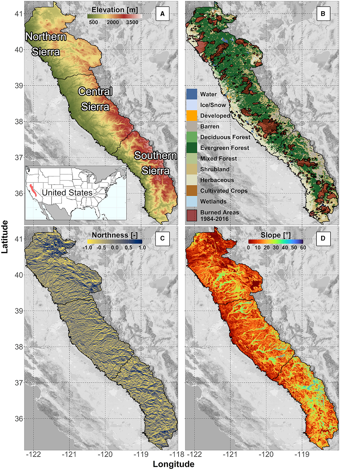
Figure 1. Sierra Nevada's study area and landscape characteristics: (A) study area's regions: northern, central, and southern Sierra, with elevation in meters above the sea level; (B) land cover classes from NLCD2011 and burned areas obtained from MTBS; (C) northness (North = 1, South = −1); (D) slope in degrees [°].

Northern Sierra is characterized by moderate elevation (elevation range from 42 to 3,071 m_asl, mean = 1,274 m_asl) and underlying volcanic and metamorphic rocks (Irwin, 1990). The average (2000–2016) annual precipitation and mean daily temperature over the NS region were 1,149 mm/yr and 10.7°C, respectively. CS is characterized by a slightly steeper elevation gradient (elevation range from 51 to 3,807 m_asl, mean = 1,259 m_asl) and by the presence of metamorphic and granitic rocks (Irwin, 1990). The precipitation averaged over the CS was 1,076 mm/yr, and the mean temperature was 11.7°C between 2000 and 2016. SS is characterized by a higher elevation (elevation range from 1,346 to 4,033 m_asl, mean = 1,837 m_asl) and by the predominance of granitic rocks (Irwin, 1990). The 2000–2016 precipitation averaged over the SS was 768 mm/yr, and the 2000–2016 average mean temperature was 9.3°C. As evident, the amount of precipitation and average temperature decrease along the north–south gradient, causing more of that precipitation to fall as snow (Bales et al., 2006).

The ecosystems in the study area follow the elevational gradient. At low elevations below approximately 1,200 m_asl, the lower montane blue oak-foothill pine woodland and savanna are dominant. This system is characterized by species, such as California foothill pines (Pinus sabiniana), oaks, and other broadleaf trees and shrubs. Low- and mid-elevations, ranging from approximately 600 to 1,800 m_asl in the NS and 800 to 1,600 m_asl in the CS and SS, are dominated by dry-mesic mixed conifer forests, like Douglas firs (Pseudotsuga menziesii), ponderosa pines (Pinus ponderosa), and California incense cedars (Calocedrus decurrens). Mesic mixed conifer forests dominate the mid-elevation region (1,400–2,500 m_asl), which has an average annual precipitation of 1,000–1,500 mm, with roughly half falling as snow. This elevation region is characterized by conifers such as white firs (Abies concolor), California incense cedars (C. decurrens), and sugar pines (P. lambertiana), with limited areas dominated by Giant Sequoias (Sequoiadendron giganteum). Ponderosa pine (P. ponderosa) and jeffrey pine (P. jeffreyi) forests can be found at higher elevations (2,200–3,000 m_asl), while red fir (A. magnifica) forests can be found mostly in areas with deep, drained soils that heavily rely on snowpack. At elevations above 3,000 m_asl, the subalpine lodgepole pine (P. contorta) is dominant (Comer et al., 2003; U.S. Geological Survey, 2016; Supplementary Figure S1).

2.2. Spatial datasets

2.2.1. Digital elevation model, land cover, and fire masks

The study area was delineated using ~30 m (1 arc-second, Figure 1A) digital elevation model (DEM, U.S. Geological Survey, 2017) and the HUC-8 watershed boundaries from the USGS Watershed Boundary Dataset, WBD (U.S. Geological Survey, 2020). We performed a terrain analysis, using TauDEM (Tarboton, 2005) and R (R Core Team, 2021), and obtained northness (North/South) and slope (Figures 1C, D).

We used land cover data from the National Land Cover Database (NLCD 2011; Dewitz, 2014) and the GAP/LANDFIRE National Terrestrial Ecosystems (U.S. Geological Survey, 2016), respectively, to select all the pixels with evergreen forests (Figure 1B) and to identify the most common plant communities. Monitoring Trends in Burn Severity (MTBS, Eidenshink et al., 2007) burned area polygons (Figure 1B) were used to mask and exclude all areas where a fire occurred between 1984 and 2016 from the further analysis. Additional information is reported in the Supplementary material (section “land cover and fire masks”).

2.2.2. Precipitation and temperatures

We obtained daily total precipitation (mm/day) and daily maximum and minimum temperatures (°C) from the parameter-elevation regressions on the independent slopes model (PRISM, Daly et al., 1994) at 30 arcsec (~800 m) resolution from 2000 to 2016. We aggregated the daily rasters to obtain the monthly average temperatures (T_m) and monthly total precipitation (P_m). P_m and T_m were then spatially downscaled from 30 arcsec (~800 m) to 0.005 degrees (~500 m) resolution using the downscaling method from Zimmermann and Roberts (2001) and Lute and Abatzoglou (2020). Additional information on the downscaling method is reported in the Supplementary material (section “precipitation and temperatures downscaling method”).

2.2.3. Monthly potential evapotranspiration

We calculated monthly potential evapotranspiration (PET_m) for each pixel, using the modified Hamon approach (1963) (adopted by Dingman, 2002; Fellows and Goulden, 2016; Roche et al., 2020): first, monthly potential evapotranspiration was estimated using the original Hamon (1963) model as follows:

$\begin{array}{ll}PE{T}_{Hamon}=29.8*n*L*\left(\frac{E_{sat}}{T_m+273.2}\right)& (1)\end{array}$

where L is the median day length (hours) (obtained using insol R package; Corripio, 2021); n is the number of days in the month; T_m is the monthly average temperature; and E_sat is the saturated vapor pressure (kPa) calculated as $E_{sat}=0.611*exp(\frac{17.3*T_m}{T_m+237.3})$. Subsequently, PET_Hamon values were adjusted using a scaling factor of 1.265 to minimize the bias (Fellows and Goulden, 2016) as follows:

$\begin{array}{ll}PE{T}_m=1.265*PE{T}_{Hamon}& (2)\end{array}$

2.2.4. Snow water equivalent

We obtained daily snow water equivalent (SWE) (2000–2016) from the Sierra Nevada snow reanalysis dataset (Margulis et al., 2015, 2016). We used changes in daily SWE (ΔSWE) to estimate monthly snow accumulation (∑SWE₊) and monthly snowmelt output (∑SWE₋). Sublimation losses and snow redistribution were not considered. In the event of a discrepancy between P_m and ∑SWE₊, we adjusted the P_m to match the differences between the two datasets. For each month m, if the total precipitation was less than the snow accumulation, we adjusted the total precipitation to match the snow accumulation.

2.2.5. Water deficit

We used the seasonality index (Leibowitz et al., 2011; Wigington et al., 2012) to explore and analyze seasonal water availability and its effect on vegetation. A monthly water surplus (S_m) can be estimated as follows:

$\begin{array}{ll}{S}_m=P_m-PE{T}_m-{SWE}_m& (3)\end{array}$

where ΔSWE_m is the monthly variation in snow water equivalent estimated as the difference between snow accumulation and melt (i.e., ∑SWE₊ − ∑SWE₋). Equation (3) accounts for the seasonality of water inputs and water demands. We defined water surplus (WS) when S_m > 0 and water deficit (WD) when S_m < 0. We calculated the yearly WD as the sum of the monthly WD for each water year. For clarity, we reversed the sign of the WD to have positive values.

We focused on the WD months to emphasize the importance of water released through snowmelt during the growing season (Figure 2). During a warmer year, a snowpack loss will reduce the water available for the vegetation during the dry summer season, inducing an additional WD. The extra WD, triggered by snowpack loss, is additionally exacerbated by an increase in evaporative demand (not reported in the conceptual Figure 2). In this study, we did not account for lateral flow and subsurface water storage.

FIGURE 2

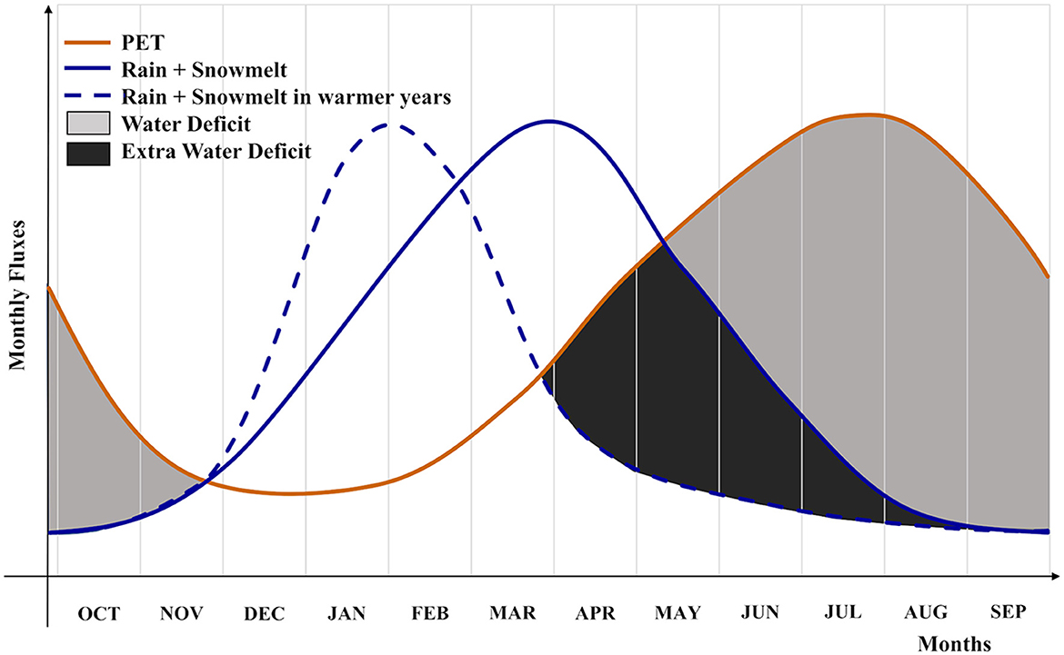
Figure 2. Conceptual diagram including the monthly potential evapotranspiration (PET, orange line); monthly water inputs (monthly rain + monthly snowmelt) in a water year characterized by an average snowpack (blue continuous line), and in a water year with a reduced snowpack (blue dashed line). Water deficit (gray areas) represents the negative difference between water inputs and potential evapotranspiration. A reduction in the snowpack, with a consequent failure in delivering the water during the spring and early summer, involves an increase in water deficit [extra water deficit (dark-gray area)].

2.2.6. Forest water stress

Normalized Difference Infrared Index (NDII) is a spectral index sensitive to vegetation canopy water content (Ceccato et al., 2002; Davidson et al., 2006). NDII is correlated with the canopy water content in different forest types (Cheng, 2007). We obtained near-infrared reflectance (NIR) and short-wave infrared reflectance (SWIR) values from MODIS/Terra 8-Day L3 Global 500 m (MOD09A1 Version 6; Vermote, 2015), from 2001 to 2016. Conversions from sinusoidal projection to NAD 83 were performed using the MODIStsp R package (Busetto and Ranghetti, 2016).

NDII was computed using the formula:

$\begin{array}{ll}NDII=\frac{NIR-SWIR}{NIR+SWIR}& (4)\end{array}$

Monthly NDII was obtained as the median of 8-day NDII. The 8-day NDII values were masked for clouds by excluding all the pixels with state quality assessment flags different than “clear.” Pixels with poor data quality were flagged as missing. While spring NDII reflects year-to-year variations in perennial evergreen and deciduous vegetation, it also includes the peak of grasses and spring deciduous vegetation productivity. Late summer season NDII is better suited to isolate the interannual response of evergreen forests (Goulden and Bales, 2019). Therefore, late summer season NDII (hereafter NDII) was calculated as an average of August, September, and October NDII.

2.3. Analysis

2.3.1. Progression of the drought

We performed an exploratory analysis to investigate the time series of average temperatures, precipitation, and snow accumulation, from 2000 to 2016, and NDII, from 2001 to 2016, for each Sierra Nevada study region (i.e., NS, CS, and SS). Consequently, we analyzed the spatial patterns of cumulative water deficit and the changes in NDII between each year from 2012 to 2016 and the pre-drought conditions, from the 2009–2011 average NDII.

2.3.2. Role of snow on water deficit

Statistical analysis was performed for each Sierra Nevada study region (i.e., NS, CS, and SS) and at six predefined elevation bands (< 1,000; 1,000–1,500; 1,500–2,000; 2,000–2,500; 2,500–3,000; and ≥3,000 m_asl). We used the lmg (Lindeman et al., 1980) relative importance analysis (ralaimpo R package; Groemping, 2006) to quantify the individual contribution (i.e., partition-explained variance) of snowmelt and potential evapotranspiration to water deficit in the linear regression equation, across the elevation bands. Additionally, 95% bootstrap confidence intervals for relative importance were obtained using 1,000 realizations.

2.3.3. Role of water deficit on NDII

We analyzed how NDII is related to water deficit to inspect regional vegetation-elevation patterns. We obtained the yearly averages for each region of NDII (response variable) and WD (explanatory variable), and we built a linear model. Accordingly, we obtained the yearly averages for each region and elevation band, and we performed an analysis of variance (ANOVA) to investigate whether the introduction of the elevation bands as an additive term significantly improved the model. Finally, we investigated the statistical significance of the interaction terms, followed by a regression coefficient pairwise comparison between the elevation bands.

2.3.4. Model building

We developed a set of three generalized additive models (GAMs) to analyze the spatiotemporal effects of multiyear cumulative water deficit on vegetation response. GAMs (Hastie and Tibshirani, 1986) are a semi-parametric extension of generalized linear models (Aalto et al., 2012; Crockett and Westerling, 2017) with a linear predictor involving a sum of smooth functions of covariates. We built separate models for NS, CS, and SS using the “Generalized Additive Models for very large datasets” R function (BAM function from mgcv package in R (Wood et al., 2014; Wood, 2017; Li and Wood, 2019).

We included four sets of smooth functions s_i in the models (Supplementary Figures S2–S4): The first set of smooth functions includes the 2-year cumulative water deficit for five plant communities' classes and accounts for the multi-year disturbance effect. The plant communities' classes include the four most common terrestrial ecological systems in each region (Table 1), while the fifth class (“other”) includes all the remaining evergreen forest pixels. Water deficit is strongly correlated (Pearson's correlation r > |0.6|) with many climatic and landscape variables. These variables are, therefore, redundant and excluded from the model. The choice of a 2-year cumulative water deficit is based on model evaluation using Akaike's and the Bayesian information criteria. The second smooth function includes latitude (lat) and longitude (long) and accounts for spatial locations and spatial correlation between neighboring pixels; the third smooth function includes slope to account for differences between steep and flat areas; the fourth smooth function includes northness to account for the differences in water demands between sunny south-faced slopes and shady north-faced slopes. These smooth functions were used to estimate the vegetation response as NDII index. For each region, the model has the following structure:

$\begin{array}{l}\begin{array}{lll}NDII\hfill & =\hfill & {\beta }_0+s_{1,j}(cumulativeWD)+s_2(lat,long)+s_3(slope)\hfill \end{array}\\ \begin{array}{ll}+\hfill & s_4(northness)+\epsilon \hfill \end{array}& (5)\end{array}$

where NDII is the response, β₀ is the intercept, s_i are smooth functions estimated by fast stable restricted maximum likelihood (fREML), and lat, long, 2-year cumulative water deficit (cumulative WD) for each of the five plant community classes j, slope, and northness are explanatory variables. We selected generalized additive models with separated terms to distinguish the influence of location, slope, northness, and 2-year cumulative WD on NDII. We used thin-plate splines that are particularly suited to interpolate climatic data (Hong et al., 2005; Aalto et al., 2012), to estimate smooth functions based on a scaled t distribution to account for heavy-tailed data (Wood et al., 2016). The models were fit to 75% of the data from 2000 to 2014, leaving the remaining 25% for validation. Consequently, we applied three increasing perturbations (+100 mm, +500 mm, and +800 mm) to the average (2002–2014) 2-year cumulative WD to test the model sensitivity of vegetation moisture response (NDII). We then used the models to simulate 2015–2016 NDII given a 2-year cumulative WD and checked simulation performance. Post-checks on the autocorrelation of model residuals were also performed. Finally, we created a set of maps for forest water stress, defined as NDII anomalies ($NDI{I}_{anomalies}=NDI{I}_{simulated}-NDI{I}_{\overline{2009:2011}}$).

TABLE 1

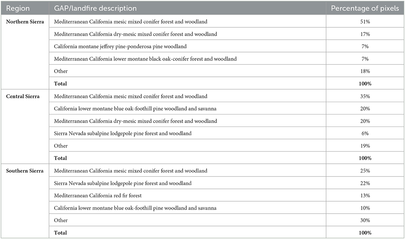
Table 1. Ecological systems used in defining the two-year cumulative Water Deficit (WD) smooths in the GAM model.

3. Results

3.1. Progression of the 2012–2015 drought

During the 2012–2015 drought, the average precipitation declined by −20% in the NS, −26% in the CS, and −40% in the SS, compared to the 2000–2016 average (Table 2). Additionally, the 2012–2015 drought was also characterized by warmer temperatures (+0.7°C in the NS, +0.6°C in the CS, and +0.7°C in the SS). The snow accumulation declined to its lowest levels [139 mm in the NS (−48%), 181 mm in the CS (−46%), and 223 mm in the SS (−48%)]. Accordingly, the NDII decreased substantially, all but at a varying rate between NS (−1%), CS (−4%), and SS (−12%), compared to the 2000–2016 average (Table 2, Figure 3). As a comparison, the 2007–2008 drought had a similar change in precipitation (−26% in the NS, −26% in the CS, and −27% in the SS). However, the duration of this drought was shorter with slightly cooler temperatures than the 2000–2016 average and thus by a modest snow accumulation decrease (−4% in the NS, −7% in the CS, and −9% in the SS). The average 2007–2008 NDII was higher in the NS (+2%) and the SS (+2%) and slightly lower in the CS (−1%) (Table 2, Supplementary Figure S5). The relationship between the change in NDII during the drought and the tree die-off (dead trees/ha) from the Forest Service Aerial Detection Survey (ADS) showed a moderate–strong correlation (Figure 4). The strength of the correlation increased as the drought progressed. In addition, NDII and basal area are related through a linear-log function (R² = 0.35, p-value < 0.001, Supplementary Figure S6) (GNN dataset; LEMMA group, 2015).

TABLE 2

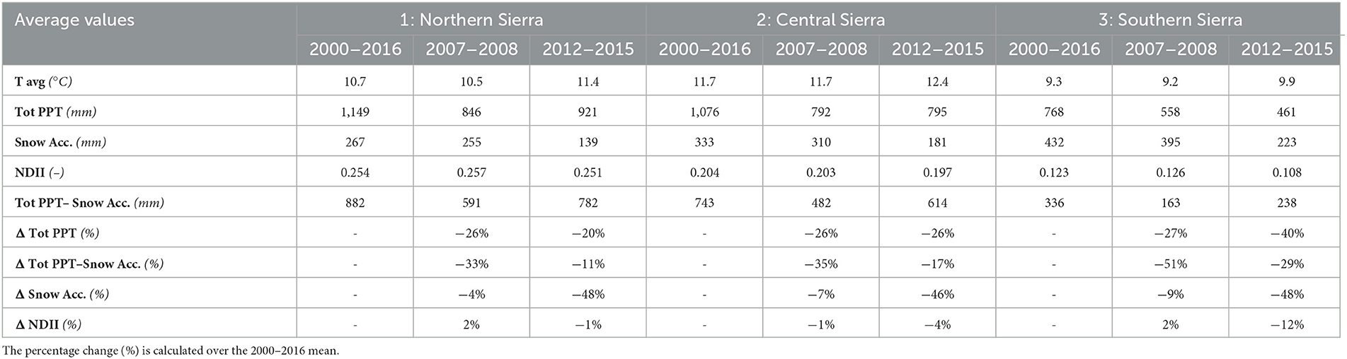
Table 2. Average values of climate and forest water stress variables for each region obtained considering all the unburned evergreen forest pixels.

FIGURE 3

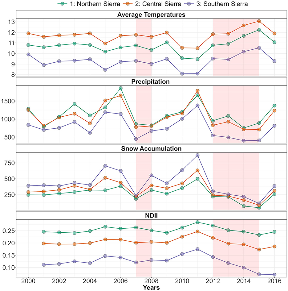
Figure 3. Time series of average temperatures, precipitation, and snow accumulation, from 2000 to 2016, and Normalized Difference Infrared Index (NDII), from 2001 to 2016, across the three study regions (NS, CS, and SS). The 2007–2008 and the 2012–2015 droughts are highlighted in red.

FIGURE 4

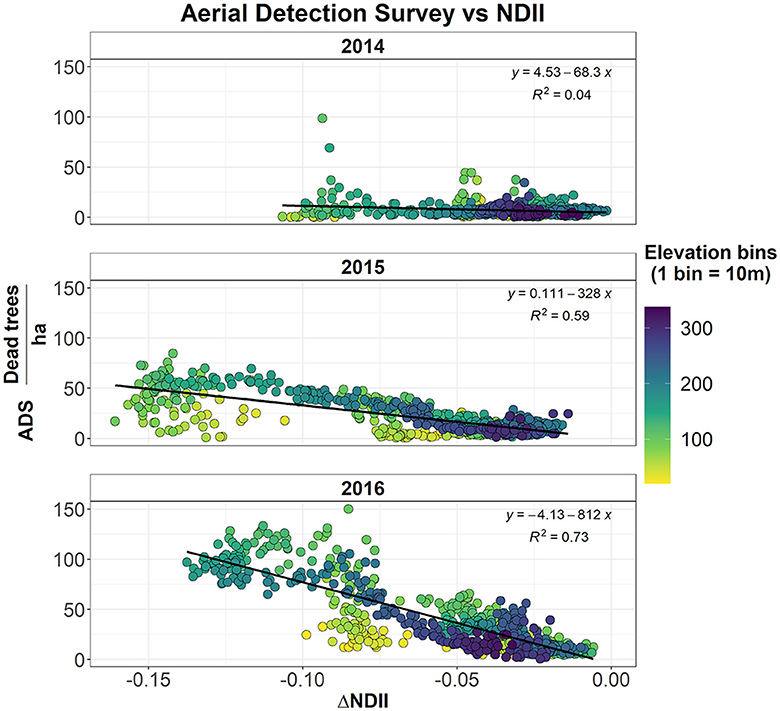
Figure 4. Relationship between the tree die-off (dead trees/ha) from the forest service Aerial Detection Survey (ADS) and the variation in NDII across different years (I = 2014, 2015, and 2016) during the drought ($NDII=NDI{I}_i-\overline{NDI{I}_{2009-2011}}$), binned by elevation.

Spatial patterns of cumulative water deficit severely increased during the drought years. Mid- and low-elevation forests exhibited higher cumulative water deficit, particularly in the SS, where the increase was more severe. The progressive decline in NDII across time is coherent with the cumulative water deficit increase, particularly in SS, which was more affected by tree mortality episodes. However, visual acuity shows a discrepancy between NDII and cumulative water deficit in the NS and the CS (Figure 5). Contrary to the SS, the increased water deficit in the NS and CS in 2015 and 2016 did not correspond to a severe decrease in the NDII.

FIGURE 5

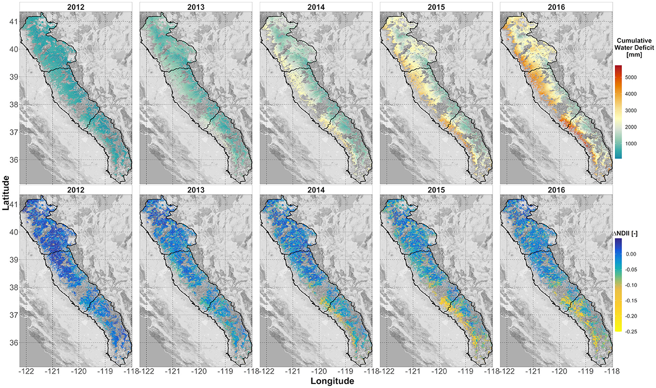
Figure 5. Progression of the drought: in the top panels, cumulative water deficit during the drought; in the bottom panels, changes in NDII between each year of the drought and the pre-drought conditions (average 2009–2011).

3.1.1. Role of snowpack

Water deficit has been used to investigate how the loss of snowpack and the increase in evaporative demand aggravated the asynchrony between water inputs and forest water demands. The relative importance analysis showed that snowmelt explained most of the variation of water deficit in the SS (43%), while in the NS and CS, PET was the dominant variable. Across the elevation gradient over the entire study area, the contribution of snowmelt to the water deficit increased with elevation, becoming the most important variable approximately 2,000–2,500 m_asl (Supplementary Figure S7).

3.1.2. Role of water deficit on NDII

The regional yearly average vegetation moisture (NDII) decreased from north to south, driven by an increase in WD (Figure 6). However, across the elevation gradient, NDII is non-linearly related to the yearly water deficit (Supplementary Figure S8). Higher elevation pixels (>2,500 m_asl) are contradistinguished by lower NDII and lower water deficit. Conversely, lower elevation pixels (< 1,000 m_asl for central and southern Sierra) are characterized by lower NDII and higher water deficit. Mid-elevation pixels are characterized by higher NDII and moderate water deficit. For each elevation band, an increase in water deficit resulted in a reduction in vegetation water content (negative regression coefficient). For all three regions, the contribution of elevation as an additive term is significant (p-value < 0.05). However, when the interaction term was included in the linear model, only a few elevation bands resulted significantly. The following pairwise comparison indicated no significant difference between the regression coefficients at different elevation bands. The same analysis was repeated using the cumulative 2-year water deficit (Supplementary Figure S9). In the southern Sierra, the 1,000–1,500 m_asl regression coefficients resulted significantly different compared to the band < 1,000 m_asl (p-value = 0.01) and the 3,000–4,035 m_asl (p-value = 0.02) regression coefficients. All the remaining regression coefficients resulted not significantly different.

FIGURE 6

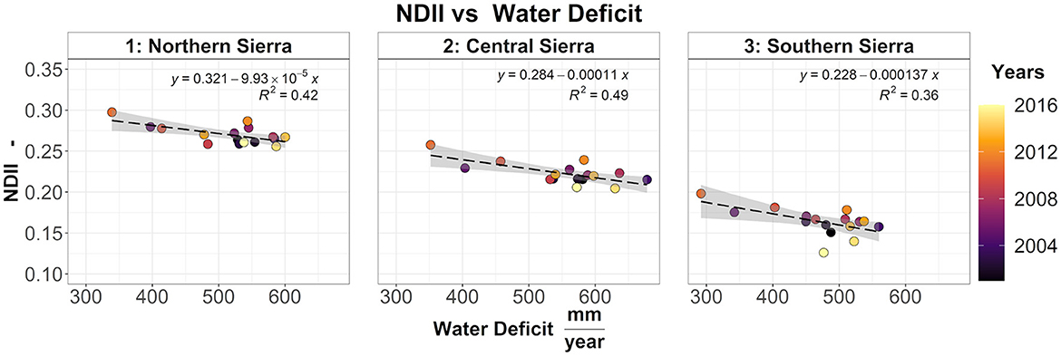
Figure 6. Relationship between NDII and water deficit across northern, central, and southern Sierra. Each dot represents the yearly average of each region.

3.2. Predicting vegetation water stress with generalized additive models

The models showed a robust performance in predicting vegetation moisture (NDII). For the southern Sierra, the coefficients of determination (R²) were 0.85, 0.84, and 0.83, respectively, for model validation, 2015 simulation, and 2016 simulation (Figure 7) and the RMSEs were 0.051, 0.069, and 0.071, respectively. Although the model had a slight tendency in overestimating the measured MODIS NDII in 2015 and 2016, most of the NDII simulations were consistent with the measured NDII (filled with lighter colors). The models can detect the distribution of the most productive region at mid-elevation [i.e., northern, central, and southern Sierra (Supplementary Figures S2–S4)]. In addition, the model captured an important partial effect of the 2-year cumulative water deficit for each ecological system, as well as a moderate partial effect of the slope and the northness.

FIGURE 7

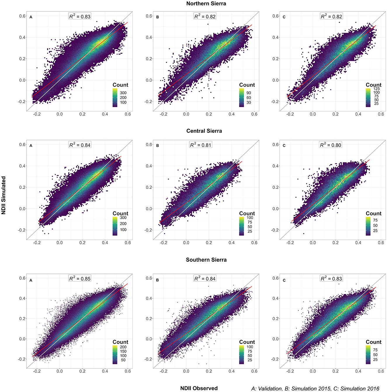
Figure 7. Model performance in the Sierra Nevada regions: NDII measured versus NDII simulated for (A) the validation pixels (25% of the pixels excluded from the training between 2001 and 2014); (B) 2015 simulation; (C) 2016 simulation.

3.3. Model sensitivity analysis

A 100-mm increase in the average 2-year cumulative WD was not translated in a conspicuous estimated vegetation moisture variation (±0.05) (Figure 8). A 500-mm perturbation caused a decrease in vegetation moisture response with spatial patterns mostly located in the SS middle-elevation forests. An 800-mm perturbation was translated into a severe decrease in vegetation moisture response across the mid-elevation forests in all the regions. Some low- and high-elevation areas were still insensitive to 2-year cumulative WD perturbations. The model sensitivity was analyzed by region and ecological system (Supplementary Figure S10). By increasing the perturbation, differences in each ecological system are evident. An 800-mm perturbation caused the most severe decrease in vegetation moisture response in the NS dry-mesic mixed conifer forests and the CC and SS mesic mixed conifer forests.

FIGURE 8

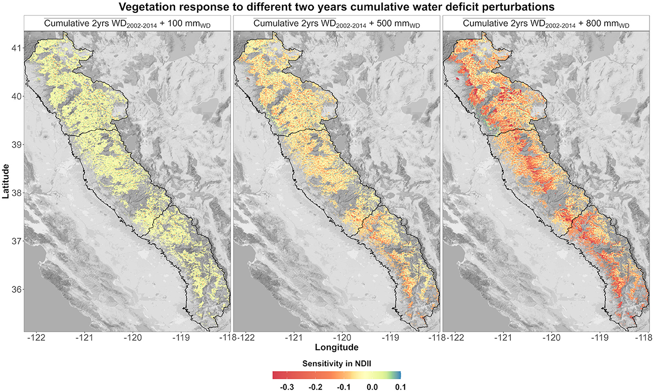
Figure 8. Modeled NDII sensitivity based on three different perturbations (100, 500, and 800 mm) applied to the average (2002–2014) 2-year cumulative WD.

3.4. Forecast maps and spatial patterns of forest water stress

The prediction of vegetation moisture (NDII) combining 2-year cumulative water deficits for each ecological system, slope, northness, and geographical coordinates allowed us to inspect the spatial pattern of forest water stress in relation to the Forest Service Aerial Detection Survey polygons. The water stress has been determined as NDII_anomalies defined as the difference between the simulated NDII for 2015 and 2016, estimated using cumulative WD and generalized additive models, and the average late summer season NDII for the period 2009–2011 (non-drought conditions). The resulting map (Figure 9) showed, for the SS region, an agreement between the spatial patterns of water stress and the 2015 Aerial Detection Survey. The difference between low tree mortality (< 10 dead trees/ha) and severe tree mortality (>100 dead trees/ha) was statistically significant (Wilcoxon rank-sum test, p-value = 0.049). Maps related to the NS and CS and 2016 SS are reported in the Supplementary Figures S11–S15.

FIGURE 9

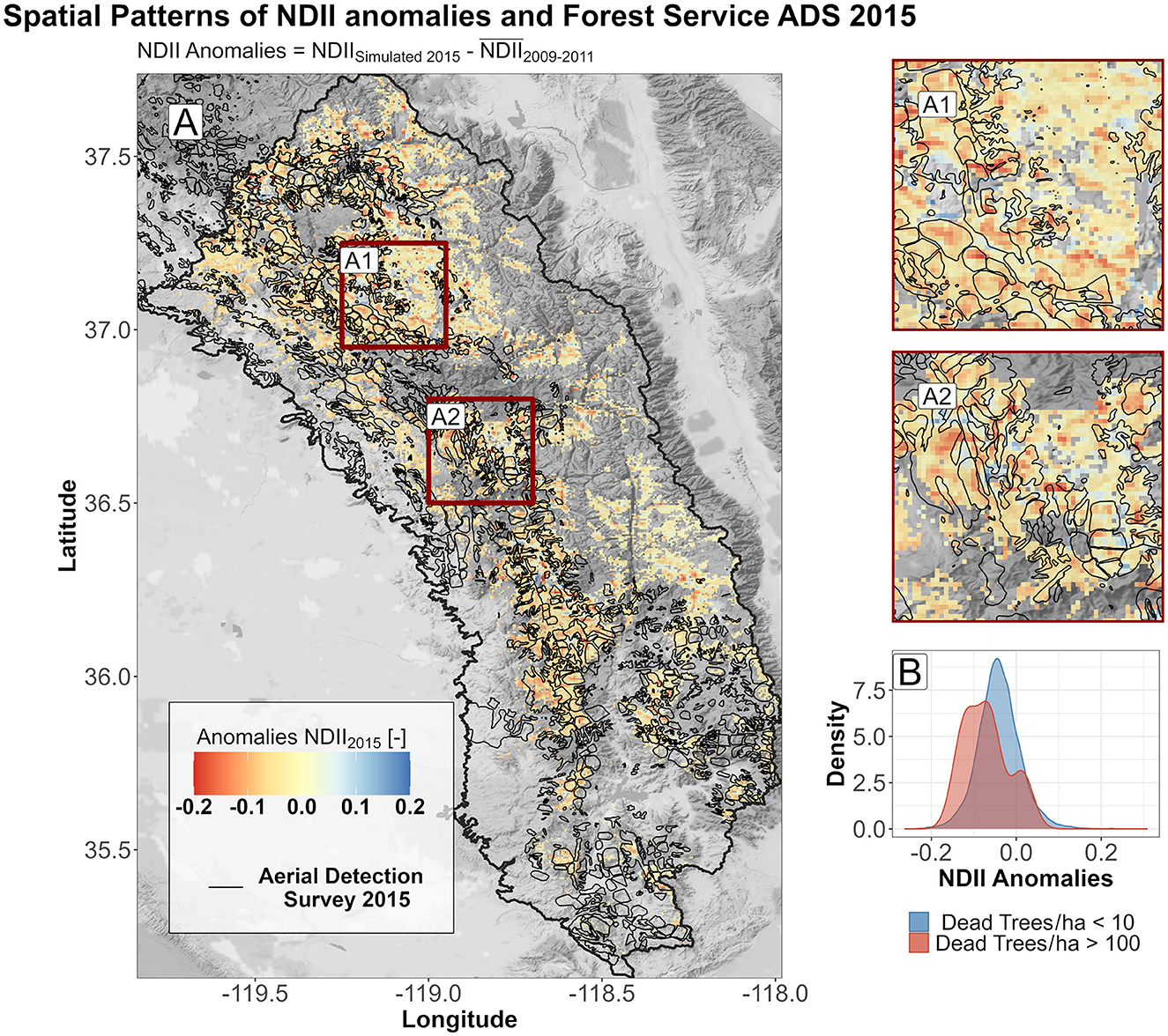
Figure 9. (A) Spatial patterns of dead trees from the Aerial Detection Survey (ADS) and anomalies in NDII for the year 2015 in the southern Sierra. A zoom into boxes A1 and A2 highlights the overlay between the ADS and the more severe simulated anomalies in NDII. (B) Comparison between density plots of anomalies in NDII for the year 2015 in the southern Sierra: In blue, pixels are characterized by low/undetected tree mortality (<10 dead trees/ha); in red, pixels are characterized by severe tree mortality (>100 dead trees/ha).

4. Discussion

Our findings suggest that snowpack loss, associated with an increase in temperatures, exacerbates vegetation water stress and consequent tree mortality episodes. The water availability necessary to maintain xylem functionality and photosynthesis is constrained by the terrestrial water storage (snowpack and subsurface water storage) and by the ability of vegetation to access it (Bales et al., 2018; Klos et al., 2018). The snowpack recharges the root zone water storage more efficiently than rain (Earman et al., 2006; Meixner et al., 2016) and provides the water necessary for the vegetation in spring and early summer when precipitation is low or absent. We used WD as a seasonal index to account for the differences in time and magnitude between water inputs and water demand. WD indicates the negative difference between monthly water inputs and monthly potential evapotranspiration (PET). The water delivered by the snowpack alleviates the WD and aids the subsurface storage in sustaining the vegetation during the growing season. Furthermore, variations in the snowpack, snowmelt timing, and temperatures directly modulate the water deficit, as confirmed by the high correlation between snowmelt and PET. As the drought propagates, an increase in WD occurred in the whole Sierra Nevada. Mid- and low-elevation forests exhibit higher cumulative water deficit across time. The increase in cumulative water deficit was particularly high in the southern Sierra region (Figure 5), which was the most affected by the 2012–2016 tree mortality episodes (U.S. Forest Service, 2016). However, in the northern and central Sierra, the increase in the cumulative deficit was not translated into vegetation water stress and tree mortality as severely as in the southern Sierra. This can be explained by the higher subsurface water available in the northern and central Sierra, as shown in previous studies (Fellows and Goulden, 2016).

Additionally, water and energy gradients across the elevation profile play a key role in the spatial distributions of forest water stress. At mid-elevation, previous studies indicate that ET is about equal to PET (Fellows and Goulden, 2016). The average yearly water deficit (pre-drought 2000–2011) in the southern Sierra for the conifer forests at mid-elevation (1,500–2,000 m_asl) was 528 mm (q_0.25 = 438 mm, q_0.75 = 607 mm). These average conditions (pre-drought) indicate that the WD was satisfied by the subsurface water storage, and it is consistent with the conifers' water withdrawal from the belowground estimated by Fellows and Goulden (2016) (30 years mean soil water drawdown of the conifers at 1,500 m_asl of ~400 mm ± ~100 mm). The 2-year cumulative WD (during dry years) at the mid-elevation region is consistent with the estimated subsurface water storage of 140 cm at the 1,100 m_asl Southern Sierra Critical Zone Observatory (SSCZO) site by Klos et al. (2018) and with the cumulative P-ET drought equilibrium of ~1,500 mm at mid-elevation obtained by Goulden and Bales (2019). At mid-elevation, NDII is higher, which indicates higher moisture content in leaves. Our study indicates that NDII and basal area are related through a linear-log function (Supplementary Figure S6). Furthermore, NDII is positively correlated with both NDVI and LAI (Goulden and Bales, 2019). Hence, the higher sensitivity (Figure 8 and Supplementary Figure S8) of the Southern Sierra NDII to the 2-year cumulative water deficit at mid-elevation indicates the higher vulnerability of the denser mid-elevation forests, consistent with Young et al. (2016) and Fettig et al. (2019).

The regional generalized additive models were trained to capture how forest moisture (NDII) varies in the landscape (using a combination of latitude, longitude, slope, and northness) based on a 2-year cumulative WD by different ecological systems, which is the unique independent variable considered that varies through time. The model results show robustness in simulating forest moisture (NDII) between regions (northern, central, and southern Sierra) and between simulated years (2015 and 2016). Our findings suggest that the difference between evaporative demand and water inputs (i.e., WD) can be used to estimate forest water stress, as NDII. The simulated anomalies in forest moisture (NDII) were reflected in the Forest Service Aerial Detection Survey (ADS) in 2015 and 2016 (Figure 9, Supplementary Figures S11–S15).

Tree species can respond differently to variations in the water balance (Hinckley et al., 1978). Some species can tolerate a larger spectrum of water availability (Lutz et al., 2010) and have different regulation strategies during dry conditions (McDowell et al., 2008). A previous study showed that across the elevation gradient, tree mortality was species-specific (Paz-Kagan et al., 2017). The inclusion of the different smooth functions in the model training helps to identify in space how pixels characterized by different vegetation composition, forest structure, and average water available respond to different levels of water deficit. Our results suggest that in the CS and SS, the mesic mixed conifer forest and the dry-mesic mixed conifer forest are the most vulnerable to cumulative water deficit variations (Supplementary Figure S10). The tree species characterizing these ecological systems are consistent with the trees least tolerant to drought reported by Kocher and Harris, 2007.

4.1. Limitations and uncertainties

Possible limitations and sources of uncertainties in this study can be identified in the following. First, the difference in the original resolution between the spatial datasets (PRISM ~800 m, MODIS ~500 m, NLCD 2011 30 m, GAP/LANDFIRE 30 m, DEM 30 m, and SWE ~90 m) may lead to inaccuracies in water deficit calculations. However, PET used in the water deficit calculation can be useful to overcome the non-availability of independent ET measurements. Second, there are temporal differences between the Aerial Detection Surveys and late summer season NDII (ADS performed during July–August 2015 and May 2016, while the late summer season NDII was derived as an average of MODIS scenes from August, September, and October). Third, in this study, we did not consider non-drought-related tree mortality (i.e., bark beetle). However, tree defenses weakened by the drought, and the consequent increase in insects and pathogens, may induce a lag in tree mortality (Das et al., 2013; Young et al., 2016). Fourth, due to the typology of the chosen statistical model, we did not account for streamflow, lateral water redistribution, and subsurface flow. This may lead to forest moisture underestimation in valleys and overestimation in runoff generation areas.

4.2. Future implications

Increases in tree mortality episodes, wildfire extent, and wildfire severity have been linked to temperature increases and lower precipitation (Crockett and Westerling, 2017). Future model projections indicate a decline and even disappearance in some parts of the snowpack in the Sierra Nevada by the end of the century (Siirila-Woodburn et al., 2021). Consequently, an increase in the summer water deficit will likely involve an increase in forest vulnerability, water stress, tree mortality, and severe wildfire risks. Higher elevation regions may be affected as well. Some locations, due to the low water storage, heavily rely on lateral flows and snowpack accumulation to support ET. The vegetation response to variations in water and energy availability will affect streamflow generation as well (Safeeq and Hunsaker, 2016). Forest management can contribute to partially mitigating such risks. A reduction in forest density can enhance forest health, increase streamflow (Tague et al., 2019), restore forest-fire resilient conditions (McKelvey and Johnston, 1992), and eventually maximize the trade-off between snow accumulation and snow ablation (Broxton et al., 2020).

5. Conclusion

We evaluated and simulated using linear regressions and regional Generalized Additive Models (GAMs) how temperature and seasonal snowpack variations can affect NDII as a proxy of forest water stress. We used water deficit as a seasonality index to inspect the critical role of mountain snowpack in reducing the mismatch between the timing of water input to the root zone and the peak forest water use under the Mediterranean climate of the Sierra Nevada. Our findings suggest that a loss of snowpack will increase the water deficit, which will lead to higher forest water stress. However, the availability of subsurface storage or lower evaporative demand can modulate the vegetation response to changes in snowpack. Consistent with previous studies, the response of the denser mid-elevation forests in the proximity of the rain–snow transition zone is more sensitive to water deficit variations. This suggests a snowpack dependence in satisfying ET requirements. We simulated forest water stress for 2015 and 2016 for the different regions (i.e., northern, central, and southern Sierra) with a range of R² between 0.80 and 0.84. The predicted spatial patterns in forest water stress were comparable with the tree die-off detected by the USDA Forest Service Aerial Detection Survey. These results can provide insight into the importance of the Sierra Nevada snowpack in a warming climate and make predictions on vulnerable areas.

Data availability statement

Publicly available datasets were analyzed in this study. This data can be found here: PRISM: https://prism.oregonstate.edu/, Sierra Nevada Snow Reanalysis: https://margulis-group.github.io/data/. Questions regarding the datasets should be directed to SC, scasirati@ucmerced.edu.

Author contributions

SC: conceptualization, methodology, investigation, analysis, visualization, writing—original draft, writing—review, and editing. MC and MS: supervision, conceptualization, resources, investigation, review, and editing. All authors contributed to the article and approved the submitted version.

Funding

This study was funded by the University of California award LFR-18-548316 and supported by INFEWS grant no. 2018-67004-24705 from the USDA National Institute of Food and Agriculture.

Conflict of interest

The authors declare that the research was conducted in the absence of any commercial or financial relationships that could be construed as a potential conflict of interest.

Publisher's note

All claims expressed in this article are solely those of the authors and do not necessarily represent those of their affiliated organizations, or those of the publisher, the editors and the reviewers. Any product that may be evaluated in this article, or claim that may be made by its manufacturer, is not guaranteed or endorsed by the publisher.

Supplementary material

The Supplementary Material for this article can be found online at: https://www.frontiersin.org/articles/10.3389/ffgc.2023.1181819/full#supplementary-material

References

Aalto, J., Pirinen, P., Heikkinen, J., and Venäläinen, A. (2012). Spatial interpolation of monthly climate data for Finland: comparing the performance of kriging and generalized additive models. Theor. Appl. Climatol. 112, 99–111. doi: 10.1007/s00704-012-0716-9

CrossRef Full Text | Google Scholar

Allen, C. D., Breshears, D. D., and McDowell, N. G. (2015). On underestimation of global vulnerability to tree mortality and forest die-off from hotter drought in the Anthropocene. Ecosphere 6, art129. doi: 10.1890/ES15-00203.1

CrossRef Full Text | Google Scholar

Bales, R. C., Goulden, M. L., Hunsaker, C. T., Conklin, M. H., Hartsough, P. C., O'Geen, A. T., et al. (2018). Mechanisms controlling the impact of multi-year drought on mountain hydrology. Scient. Rep. 8, 1. doi: 10.1038/s41598-017-19007-0

PubMed Abstract | CrossRef Full Text | Google Scholar

Bales, R. C., Molotch, N. P., Painter, T. H., Dettinger, M. D., Rice, R., and Dozier, J. (2006). Mountain hydrology of the western United States. Water Resour. Res. 42, 8. doi: 10.1029/2005WR004387

CrossRef Full Text | Google Scholar

Barnett, T. P., Adam, J. C., and Lettenmaier, D. P. (2005). Potential impacts of a warming climate on water availability in snow-dominated regions. Nature 438, 303–309. doi: 10.1038/nature04141

PubMed Abstract | CrossRef Full Text | Google Scholar

Bedsworth, L., Cayan, D., Franco, G., Fisher, L., and Ziaja, S. (2018). Statewide Summary Report. California's Fourth Climate Change Assessment. Publication number: SUMCCCA4-2018-013

Google Scholar

Broxton, P. D., Leeuwen, W. J. D., and Biederman, J. A. (2020). Forest cover and topography regulate the thin, ephemeral snowpacks of the semiarid Southwest United States. Ecohydrology 13, 4. doi: 10.1002/eco.2202

CrossRef Full Text | Google Scholar

Busetto, L., and Ranghetti, L. (2016). MODIStsp: An R package for automatic preprocessing of MODIS Land Products time series. Comput. Geosci. 97, 40–48. doi: 10.1016/j.cageo.2016.08.020

CrossRef Full Text | Google Scholar

Ceccato, P., Gobron, N., Flasse, S., Pinty, B., and Tarantola, S. (2002). Designing a spectral index to estimate vegetation water content from remote sensing data: Part 1. Remote Sens. Environ. 82, 188–197. doi: 10.1016/S0034-4257(02)00037-8

CrossRef Full Text | Google Scholar

Cheng, Y.-B. (2007). Relationships between Moderate Resolution Imaging Spectroradiometer water indexes and tower flux data in an old growth conifer forest. J. Appl. Rem. Sens. 1, 013513. doi: 10.1117/1.2747223

CrossRef Full Text | Google Scholar

Comer, P., Faber-Langendoen, D., Evans, R., Gawler, S., Josse, C., Kittel, G., et al. (2003). Ecological systems of the United States: a working classification of US terrestrial systems. Arlington, VA: NatureServe.

Google Scholar

Corripio, J. G. (2021). insol: Solar Radiation. R package version 1.2.2. Available online at: https://CRAN.R-project.org/package=insol (accessed July 31, 2022).

Google Scholar

Crockett, J. L., and Westerling, A. L. (2017). Greater temperature and precipitation extremes intensify western U.S. droughts, wildfire severity, and sierra nevada tree mortality. J. Clim. 31, 341–354. doi: 10.1175/JCLI-D-17-0254.1

CrossRef Full Text | Google Scholar

Daly, C., Neilson, R. P., and Phillips, D. L. (1994). A statistical-topographic model for mapping climatological precipitation over mountainous terrain. J. Appl. Meteorol. 33, 140–158. doi: 10.1175/1520-0450(1994)033<0140:ASTMFM>2.0.CO;2

CrossRef Full Text | Google Scholar

Das, A. J., Stephenson, N. L., Flint, A., Das, T., and van Mantgem, P. J. (2013). Climatic correlates of tree mortality in water- and energy-limited forests. PLoS ONE 8, e69917. doi: 10.1371/journal.pone.0069917

PubMed Abstract | CrossRef Full Text | Google Scholar

Davidson, A., Wang, S., and Wilmshurst, J. (2006). Remote sensing of grassland–shrubland vegetation water content in the shortwave domain. Int. J. Appl. Earth Observ. Geoinform. 8, 225–236. doi: 10.1016/j.jag.2005.10.002

CrossRef Full Text | Google Scholar

Dettinger, M. D., and Anderson, M. L. (2015). Storage in California's reservois and snowpack in this time of drought. San Francisco Estuary Watershed Sci. 13, 2. doi: 10.15447/sfews.2015v13iss2art1

CrossRef Full Text | Google Scholar

Dewitz, J. (2014). National Land Cover Database (NLCD) 2011 Land Cover Conterminous United States [Data set]. U.S. Geological Survey.

Google Scholar

Dingman, S. L. (2002). Physical Hydrology. 2nd Edn. Upper Saddle River, NJ: Prentice Hall.

Google Scholar

Earman, S., Campbell, A. R., Phillips, F. M., and Newman, B. D. (2006). Isotopic exchange between snow and atmospheric water vapor: Estimation of the snowmelt component of groundwater recharge in the southwestern United States. J. Geophys. Res. 111, D9. doi: 10.1029/2005JD006470

CrossRef Full Text | Google Scholar

Eidenshink, J., Schwind, B., Brewer, K., Zhu, Z.-L., Quayle, B., and Howard, S. (2007). A project for monitoring trends in burn severity. Fire Ecol. 3, 3–21. doi: 10.4996/fireecology.0301003

CrossRef Full Text | Google Scholar

Fellows, A. W., and Goulden, M. L. (2016). Mapping and understanding dry season soil water drawdown by California montane vegetation. Ecohydrology 10, e1772. doi: 10.1002/eco.1772

CrossRef Full Text | Google Scholar

Fettig, C. J., Mortenson, L. A., Bulaon, B. M., and Foulk, P. B. (2019). Tree mortality following drought in the central and southern Sierra Nevada, California, U.S. Forest Ecol. Manage. 432, 164–178. doi: 10.1016/j.foreco.2018.09.006

PubMed Abstract | CrossRef Full Text | Google Scholar

Garcia, E. S., and Tague, C. L. (2015). Subsurface storage capacity influences climate–evapotranspiration interactions in three western United States catchments. Hydrol. Earth Syst. Sci. 19, 4845–4858. doi: 10.5194/hess-19-4845-2015

CrossRef Full Text | Google Scholar

Goulden, M. L., and Bales, R. C. (2019). California forest die-off linked to multi-year deep soil drying in 2012–2015 drought. Nat. Geosci. 12, 632–637. doi: 10.1038/s41561-019-0388-5

CrossRef Full Text | Google Scholar

Groemping, U. (2006). Relative Importance for Linear Regression in R: The Package relaimpo. J. Stat. Softw. 17, 1–27. doi: 10.18637/jss.v017.i01

CrossRef Full Text | Google Scholar

Hamon, W. (1963). Computation of direct runoff amounts from storm rainfall. Int. Assoc. Sci. Hydrol. Publ. 63, 52–62.

Google Scholar

Hardisky, M. A., Klemas, V., and Smart, R. M. (1983). The influence of soilsalinity, growth form, and leaf moisture on the spectral radiance of Spartina alterniflora canopies. Photogram. Eng. Rem. Sens. 49, 77–83.

Google Scholar

Hastie, T., and Tibshirani, R. (1986). Generalized additive models. Stat. Sci. 1, 3. doi: 10.1214/ss/1177013604

CrossRef Full Text | Google Scholar

Hinckley, T. M., Lassoie, J. P., and Running, S. W. (1978). Temporal and spatial variations in water status of forest trees. Forest Sci. 24, 1–72.

Google Scholar

Hong, Y., Nix, H. A., Hutchinson, M. F., and Booth, T. H. (2005). Spatial interpolation of monthly mean climate data for China. Int. J. Climatol. 25, 1369–1379. doi: 10.1002/joc.1187

CrossRef Full Text | Google Scholar

Irwin, W. P. (1990). “Geology and plate-tectonic development,” in R. E. Wallace, ed., The San Andreas Fault System: U.S. Geological Survey Professional 61–80. Available online at: https://pubs.usgs.gov/pp/1990/1515/

Google Scholar

Kimes, D. S., Markham, B. L., Tucker, C. J., and McMurtrey, J. E. III. (1981). Temporal relationships between spectral response and agronomic variables of a corn canopy. Remote Sens. Environ. 11, 401–411. doi: 10.1016/0034-4257(81)90037-7

CrossRef Full Text | Google Scholar

Klos, P. Z., Goulden, M. L., Riebe, C. S., Tague, C. L., O'Geen, A. T., Flinchum, B. A., et al. (2018). Subsurface plant-accessible water in mountain ecosystems with a Mediterranean climate. WIREs Water 5, 3. doi: 10.1002/wat2.1277

CrossRef Full Text | Google Scholar

Knowles, N., Dettinger, M. D., and Cayan, D. R. (2006). Trends in Snowfall versus Rainfall in the Western United States. J. Climate 19, 4545–4559. doi: 10.1175/JCLI3850.1

CrossRef Full Text | Google Scholar

Kocher, S. D., and Harris, R. (2007). Forest Stewardship Series 5: Tree Growth and Competition. University of California, Agriculture and Natural Resources. doi: 10.3733/ucanr.8235

CrossRef Full Text | Google Scholar

Leibowitz, S. G., Wigington, J.r. P. J, Comeleo, R. L., and Ebersole, J. L. (2011). A temperature-precipitation-based model of thirty-year mean snowpack accumulation and melt in Oregon, USA. Hydrol. Proces. 26, 741–759. doi: 10.1002/hyp.8176

CrossRef Full Text | Google Scholar

LEMMA group (2015). GNN structure (species-size) maps. Available online at: http://lemma.forestry.oregonstate.edu/data/structure-maps (accessed May 17, 2017).

Google Scholar

Li, Z., and Wood, S. N. (2019). Faster model matrix crossproducts for large generalized linear models with discretized covariates. Stat. Comput. 30, 19–25. doi: 10.1007/s11222-019-09864-2

CrossRef Full Text | Google Scholar

Lindeman, R. H., Merenda, P. F., and Gold, R. Z. (1980). Introduction to Bivariate and Multivariate Analysis. Glenview, IL: Scott, Foresman.

Google Scholar

Lute, A. C., and Abatzoglou, J. T. (2020). Best practices for estimating near-surface air temperature lapse rates. Int. J. Climatol. 41, S1. doi: 10.1002/joc.6668

CrossRef Full Text | Google Scholar

Lutz, J. A., van Wagtendonk, J. W., and Franklin, J. F. (2010). Climatic water deficit, tree species ranges, and climate change in Yosemite National Park. J. Biogeogr. 37, 936–950. doi: 10.1111/j.1365-2699.2009.02268.x

CrossRef Full Text | Google Scholar

Mann, M. E., and Gleick, P. H. (2015). “Climate change and California drought in the 21st century,” in Proceedings of the National Academy of Sciences 112, 3858–3859. doi: 10.1073/pnas.1503667112

PubMed Abstract | CrossRef Full Text | Google Scholar

Margulis, S. A., Cortés, G., Girotto, M., and Durand, M. (2016). A landsat-era sierra nevada snow reanalysis (1985–2015). J. Hydrometeorol. 17, 1203–1221. doi: 10.1175/JHM-D-15-0177.1

CrossRef Full Text | Google Scholar

Margulis, S. A., Girotto, M., Cortés, G., and Durand, M. (2015). A particle batch smoother approach to snow water equivalent estimation. J. Hydrometeorol. 16, 1752–1772. doi: 10.1175/JHM-D-14-0177.1

CrossRef Full Text | Google Scholar

McDowell, N., Pockman, W. T., Allen, C. D., Breshears, D. D., Cobb, N., Kolb, T., et al. (2008). Mechanisms of plant survival and mortality during drought: why do some plants survive while others succumb to drought? New Phytol. 178, 719–739. doi: 10.1111/j.1469-8137.2008.02436.x

PubMed Abstract | CrossRef Full Text | Google Scholar

McKelvey, K. S., and Johnston, J. D. (1992). “Historical perspectives on forests of the Sierra Nevada and the transverse ranges of southern California; forest conditions at the turn of the century,” in The California spotted owl: a technical assessment of its current status (Albany, CA: Pacific Southwest Research Station, Forest Service, U.S. Department of Agriculture) 225–246.

Google Scholar

Meixner, T., Manning, A. H., Stonestrom, D. A., Allen, D. M., Ajami, H., Blasch, K. W., et al. (2016). Implications of projected climate change for groundwater recharge in the western United States. J. Hydrol. 534, 124–138. doi: 10.1016/j.jhydrol.2015.12.027

CrossRef Full Text | Google Scholar

Mote, P. W., Hamlet, A. F., Clark, M. P., and Lettenmaier, D. P. (2005). Declining mountain snowpack in western North America. Bull. Am. Meteorol. Soc. 86, 39–50. doi: 10.1175/BAMS-86-1-39

CrossRef Full Text | Google Scholar

Paz-Kagan, T., Brodrick, P. G., Vaughn, N. R., Das, A. J., Stephenson, N. L., Nydick, K. R., et al. (2017). What mediates tree mortality during drought in the southern Sierra Nevada? Ecol. Applic. 27, 2443–2457. doi: 10.1002/eap.1620

PubMed Abstract | CrossRef Full Text | Google Scholar

R Core Team (2021). R: A Language and Environment for Statistical Computing. Vienna, Austria. Available online at: https://www.R-project.org (accessed July 31, 2022).

Google Scholar

Restaino, C., Young, D. J. N., Estes, B., Gross, S., Wuenschel, A., Meyer, M., et al. (2019). Forest structure and climate mediate drought-induced tree mortality in forests of the Sierra Nevada, USA. Ecol. Appl. 29, e01902. doi: 10.1002/eap.1902

PubMed Abstract | CrossRef Full Text | Google Scholar

Roche, J. W., Ma, Q., Rungee, J., and Bales, R. C. (2020). Evapotranspiration Mapping for Forest Management in California's Sierra Nevada. Front. Forests Global Change 3, 69. doi: 10.3389/ffgc.2020.00069

CrossRef Full Text | Google Scholar

Safeeq, M., and Hunsaker, C. T. (2016). Characterizing runoff and water yield for headwater catchments in the southern sierra nevada. JAWRA J. Am. Water Resour. Assoc. 52, 1327–1346. doi: 10.1111/1752-1688.12457

CrossRef Full Text | Google Scholar

Safeeq, M., Shukla, S., Arismendi, I., Grant, G. E., Lewis, S. L., and Nolin, A. (2015). Influence of winter season climate variability on snow-precipitation ratio in the western United States. Int. J. Climatol. 36, 3175–3190. doi: 10.1002/joc.4545

CrossRef Full Text | Google Scholar

Siirila-Woodburn, E. R., Rhoades, A. M., Hatchett, B. J., Huning, L. S., Szinai, J., Tague, C., et al. (2021). A low-to-no snow future and its impacts on water resources in the western United States. Nat. Rev. Earth Environ. 2, 800–819. doi: 10.1038/s43017-021-00219-y

CrossRef Full Text | Google Scholar

Swain, D. L., Langenbrunner, B., Neelin, J. D., and Hall, A. (2018). Increasing precipitation volatility in twenty-first-century California. Nat. Clim. Change 8, 427–433. doi: 10.1038/s41558-018-0140-y

CrossRef Full Text | Google Scholar

Tague, C. L., Moritz, M., and Hanan, E. (2019). The changing water cycle: The eco-hydrologic impacts of forest density reduction in Mediterranean (seasonally dry) regions. WIREs Water 6, 4. doi: 10.1002/wat2.1350

CrossRef Full Text | Google Scholar

Tarboton, D. G. (2005). Terrain analysis using digital elevation models (TauDEM). Utah State Univ. Logan 3012, 2018.

PubMed Abstract | Google Scholar

Thorne, J. H., Boynton, R. M., Flint, L. E., and Flint, A. L. (2015). The magnitude and spatial patterns of historical and future hydrologic change in California's watersheds. Ecosphere 6, art24. doi: 10.1890/ES14-00300.1

CrossRef Full Text | Google Scholar

Trujillo, E., Molotch, N. P., Goulden, M. L., Kelly, A. E., and Bales, R. C. (2012). Elevation-dependent influence of snow accumulation on forest greening. Nat. Geosci. 5, 705–709. doi: 10.1038/ngeo1571

CrossRef Full Text | Google Scholar

U.S. Forest Service (2016). U.S. Forest Service Pacific Southwest Region Forest Health Protection Aerial Detection Survey. Available online at: https://www.fs.usda.gov/detail/r5/forest-grasslandhealth/?cid=fsbdev3_046696 (accessed December 8, 2021).

Google Scholar

U.S. Geological Survey (2016). GAP/LANDFIRE National Terrestrial Ecosystems 2011: U.S. Geological Survey data release.

Google Scholar

U.S. Geological Survey (2017) 1 Arc-second Digital Elevation Models (DEMs) - USGS National Map 3DEP Downloadable Data Collection. U.S. Geological Survey.

Google Scholar

U.S. Geological Survey (2020). USGS watershed boundary dataset (WBD) for 2-digit Hydrologic unit - 18 (published 20201204). U.S. Geological Survey (USGS).

Google Scholar

Vermote, E. (2015). MOD09A1 MODIS/Terra Surface Reflectance 8-Day L3 Global 500m SIN Grid V006 [Data set]. NASA EOSDIS Land Processes DAAC.

Google Scholar

Wigington, P. J., Leibowitz, S. G., Comeleo, R. L., and Ebersole, J. L. (2012). Oregon Hydrologic Landscapes: A Classification Framework1. JAWRA J. Am. Water Resour. Assoc. 49, 1, 163–182. doi: 10.1111/jawr.12009

CrossRef Full Text | Google Scholar

Williams, A. P., Seager, R., Abatzoglou, J. T., Cook, B. I., Smerdon, J. E., and Cook, E. R. (2015). Contribution of anthropogenic warming to California drought during 2012–2014. Geophys. Res. Lett. 42, 6819–6828. doi: 10.1002/2015GL064924

CrossRef Full Text | Google Scholar

Wilson, E. H., and Sader, S. A. (2002). Detection of forest harvest type using multiple dates of Landsat TM imagery. Remote Sens. Environ. 80, 385–396. doi: 10.1016/S0034-4257(01)00318-2

CrossRef Full Text | Google Scholar

Wood, S. N. (2017). Generalized Additive Models. Chapman and Hall/CRC. doi: 10.1201/9781315370279

CrossRef Full Text | Google Scholar

Wood, S. N., Goude, Y., and Shaw, S. (2014). Generalized additive models for large data sets. J. R. Stat. Soc. 64, 139–155. doi: 10.1111/rssc.12068

CrossRef Full Text | Google Scholar

Wood, S. N., Pya, N., and Säfken, B. (2016). Smoothing Parameter and Model Selection for General Smooth Models. J. Am. Stat. Assoc. 111, 1548–1563. doi: 10.1080/01621459.2016.1180986

CrossRef Full Text | Google Scholar

Yilmaz, M. T., Hunt, E. R. Jr., and Jackson, T. J. (2008). Remote sensing of vegetation water content from equivalent water thickness using satellite imagery. Remote Sens. Environ. 112, 2514–2522. doi: 10.1016/j.rse.2007.11.014

CrossRef Full Text | Google Scholar

Young, D. J. N., Stevens, J. T., Earles, J. M., Moore, J., Ellis, A., Jirka, A. L., et al. (2016). Long-term climate and competition explain forest mortality patterns under extreme drought. Ecol. Lett. 20, 78–86. doi: 10.1111/ele.12711

PubMed Abstract | CrossRef Full Text | Google Scholar

Zimmermann, N. E., and Roberts, D. W. (2001). Final report of the MLP climate and biophysical mapping project. Swiss Federal Research Institute WSL/Utah State University Birmensdorf, Switzerland/Logan, USA 18.

Google Scholar