Precise and unbiased biomass estimation from GEDI data and the US Forest Inventory

Atmospheric CO₂ concentrations are dependent on land-atmosphere carbon fluxes resultant from forest dynamics and land-use changes. These fluxes are not well-constrained, in part because reliable baseline estimates of forest carbon stocks and the associated uncertainties are lacking. NASA's Global Ecosystem Dynamics Investigation (GEDI) produces estimates of aboveground biomass density (AGBD) that are unique because GEDI's hybrid estimation framework enables formal uncertainty calculations that accompany the biomass estimates. However, GEDI's estimates are not without issue; a recent validation using design-based AGBD estimates from the US Forest Inventory and Analysis (FIA) program revealed systematic differences between GEDI and FIA estimates within a hexagon tessellation of the continental United States. Here, we explored these differences and identified two issues impacting GEDI's estimation process: incomplete filtering of low quality GEDI observations and regional biases in GEDI's footprint-level biomass models. We developed a solution to each, in the form of improved data filtering and GEDI-FIA fusion AGBD models, developed in a scale-invariant small area estimation framework, that were compatible with hybrid estimation. We calibrated 10 regional Fay-Herriot models at the hexagon scale for application at the unit scale of GEDI footprints, for which we provide a mathematical justification and empirical testing of the models' scale-invariance. These models predicted realistic distributions of unit level AGBD, with equal or improved performance relative to GEDI's L4A models for all regions. We then produced GEDI-FIA fusion estimates that were more precise than the FIA estimates and resulted in a bias reduction of 86.7% relative to the original GEDI estimates: 19.3% due to improved data filtering and 67.5% due to the new AGBD models. Our findings indicate that (1) small area estimation models trained in a scale-invariant framework can produce realistic predictions of AGBD, and (2) there is substantial spatial variability in the relationship between GEDI forest structure metrics and AGBD. This work is a step toward achieving reliable baseline forest carbon stocks, provides a viable methodology for training remote sensing biomass models, and may serve as a reference for other investigations of GEDI AGBD estimates.

1. Introduction

NASA's Global Ecosystem Dynamics Investigation (GEDI) is the first spaceborne mission designed specifically to estimate aboveground biomass (Dubayah R. et al., 2020). GEDI is a multi-beam waveform lidar mounted on the International Space Station that directly measures forest structure within footprints 25 m wide along eight reference ground tracks. GEDI's sole observable is a reflected waveform, from which forest structure metrics are calculated. These waveforms enable above ground biomass density (AGBD) mapping within a regular spatial grid or jurisdictional boundaries, as follows. First, GEDI's level 2A (L2A) signal processing algorithms are applied to each waveform to calculate metrics representative of forest structure attributes (Hofton et al., 2020). Second, GEDI's level 4A (L4A) footprint level AGBD models use the metrics to predict AGBD within the waveform footprint (Kellner et al., 2022). Third, hybrid inference estimators are applied to the footprint level AGBD predictions produce estimates of mean AGBD and uncertainty in the form of a standard error of the mean estimate (Healey et al., 2022). Throughout this paper we refer to these steps collectively as the GEDI's “estimation process”, to individual GEDI waveforms as “observations”, and to the derived mean estimates of AGBD in step three as “estimates”.

Hybrid inference (hereafter “hybrid”) is an established method to estimate AGBD and its uncertainty from lidar remote sensing (Healey et al., 2012; Margolis et al., 2015; Nelson et al., 2017). Hybrid is valuable because it provides a formal estimate of the mean estimate's uncertainty, which improves the utility of the resultant map. GEDI's AGBD maps are unique relative to most other global biomass maps (e.g., Saatchi et al., 2011; Avitabile et al., 2016; Santoro and Cartus, 2021) because the hybrid variance estimators account for both sampling and model uncertainty in a transparent manner, compared to ad hoc methods of uncertainty characterization that do not rely on a statistical framework. GEDI's AGBD estimation process was designed to satisfy the assumptions necessary for hybrid inference; (1) the GEDI sample approximates a simple random cluster sample within each spatial estimation unit, in which each laser ground track is a cluster sample, and there are at least two cluster samples in each spatial unit; (2) the L4A models are properly specified and unbiased throughout the entire area in which they are applied; and (3) over large-enough areas the residual error from the L4A models sums to zero (Patterson et al., 2019).

While the first and third assumptions were addressed by Patterson et al. (2019) during GEDI's pre-launch phase, the extent to which the L4A models are unbiased everywhere is not well-established (Dubayah et al., 2022b; Duncanson L. et al., 2022). This possibility is acknowledged by Duncanson L. et al. (2022), and represents a substantial challenge in developing globally representative prediction models due to geographic gaps in training data used to calibrate the L4A models that must be transferable to entire continents. Such an assessment requires validation of GEDI's AGBD estimates with independent reference data, however standardized reference data does not exist to validate a global biomass map at 1 km resolution (Duncanson L. et al., 2021). Instead, McRoberts et al. (2019) outline a strategy for local validation of global biomass maps using design-based estimates of biomass from a national forest inventory at the same spatial scale of the global map. Since the true AGBD for an estimation unit is unknown, the authors suggest validation by comparing population estimates, characterizing the difference between the reference estimate and the remote sensing estimate in a probabilistic manner.

Such a validation of GEDI's AGBD estimates was recently performed. The United States Forest Inventory and Analysis (FIA) program maintains a random sample of national forest inventory plots, from which Menlove and Healey (2020) produced post-stratified design-based reference estimates of AGBD within an equal area hexagon tessellation (~640 km², n = 12,550) covering the continental United States. Generated specifically for validating remote sensing biomass maps, the FIA hexagon reference estimates were used by Dubayah et al. (2022b) to validate an analogous set of GEDI hexagon AGBD estimates. The analysis exhibited strong spatial patterns of both positive and negative systematic differences between the GEDI and FIA reference estimates that were unlikely due to chance. Here, we assume the FIA reference estimates are unbiased, and that systematic differences between the GEDI and FIA estimates are caused by issues biasing GEDI's estimation process. If maps of biomass from remote sensing are to be used more widely, it is important that differences relative to well-designed national forest inventory networks be reconciled.

The goal of this paper is to mitigate the primary issues that adversely affect GEDI's overall biomass estimation process. We hypothesize these issues to be (1) incomplete filtering of low-quality observations not suited for AGBD estimation, and (2) regional misspecification of the L4A footprint level AGBD prediction models. Specifically, our objectives are:

1. To identify and remove GEDI observations not suited for biomass estimation, that are not caught by GEDI's standard quality filtering.

2. Develop unbiased footprint level AGBD models that may be used within GEDI's hybrid inference framework.

3. Quantify the overall improvement in GEDI AGBD estimation, relative to the FIA estimates, brought by these advancements to GEDI's estimation process.

While our approach is aimed at improving GEDI's overall AGBD estimation process, the changes we make in the form of improved quality filtering and new footprint level AGBD models only affect the inputs to the population estimation method of hybrid inference, and not the actual hybrid mean and variance estimators put forth by Patterson et al. (2019).

2. Materials and methods

First, we repeated Dubayah et al.'s (2022b) validation of GEDI hexagon estimates to highlight regions of systematic difference relative to the FIA estimates, which informed our hypotheses about the two factors adversely impacting GEDI's original AGBD hexagon estimates; incomplete quality filtering and footprint AGBD model misspecification (Figure 1). We designed and applied additional quality filters to produce a set of GEDI hexagon AGBD estimates using hybrid inference that excluded the observations flagged by our additional filters, which we call “filtered” GEDI estimates. Next, we developed new footprint AGBD models using GEDI-FIA fusion in a scale-invariant small area (SISA) estimation framework, which we refer to as the SISA models. We calibrated Fay-Herriot small area estimation models at an aggregated scale, regressing the FIA hexagon estimates of AGBD against hexagon aggregations of GEDI metrics in such a way that the resultant equations were largely unbiased and applicable at the footprint level. We also developed a theoretical justification and validation of these models given the available data. We then applied the SISA models to the GEDI observations resulting in new footprint level AGBD predictions, from which we generated a new set of GEDI hexagon AGBD estimates again using hybrid inference, which we refer to as “fusion” estimates. We also generated “fusion” estimates at the 1 km scale, based on the flexible nature of GEDI's hybrid estimation framework. Lastly, we compared the “filtered” and “fusion” GEDI-based estimates with the estimates from Dubayah et al. (2022b) (hereafter the “original” estimates) to quantify the improvements that our filtering and modeling methods had on GEDI's AGBD estimates, relative to the design-based FIA reference estimates. In the following sections we first outline the GEDI and FIA data sources used in our work, and our method of comparing the GEDI and FIA estimates to identify non-random systematic differences. We then catalog the steps taken to develop, implement, and assess our solutions to both the data filtering and model misspecification issues.

FIGURE 1

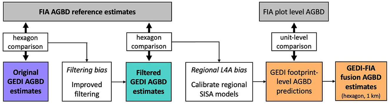
Figure 1. Methodological overview. We began by comparing the original GEDI and FIA hexagon estimates, and hypothesized that inclusion of GEDI observations not suited for biomass estimation were causing systematic differences relative to the FIA estimates. We developed methods to identify those observations, removed them from GEDI's biomass estimation process, and generated an updated set of “filtered” GEDI estimates. A comparison of the filtered GEDI and FIA hexagon estimates revealed a second source of difference between GEDI and FIA estimates, which we hypothesized were due to regional L4A model biases. In response, we developed a scale-invariant, small area (SISA) estimation framework to calibrate new GEDI footprint level AGBD models using GEDI-FIA fusion. When applied to the GEDI observations, the SISA models resulted in mostly unbiased predictions that were more accurate and realistic than the L4A models. We then used the SISA predictions to generate updated “fusion” GEDI estimates, at both the hexagon and 1 km scale.

2.1. GEDI data and algorithms

The GEDI data used were the L2A footprint level waveform metrics (Dubayah S. et al., 2020) and the L4A footprint level AGBD predictions (Dubayah R. et al., 2021), collected between April 18th 2019 and May 11 2022. We applied the quality filtering criteria put forth in Dubayah et al. (2022b) to ensure we used only the highest quality observations for biomass estimation (see Supplementary material), and generated the set of “original” GEDI hexagons estimates using the exact same hybrid inference methods as in Dubayah et al. (2022b). After developing and implementing both our additional filtering criteria and the SISA footprint level AGBD models, we again used hybrid inference to generate the “filtered” and “fusion” GEDI hexagon level biomass estimates. This was done using the same code base and hybrid estimators used to produce GEDI's L4B data products (Dubayah et al., 2022a,b), with slight modifications to accommodate our changes to the estimation process. We also used the 1 km GEDI L4B gridded biomass product in comparisons with our 1 km gridded fusion estimates (Dubayah et al., 2022a).

2.2. FIA data

The FIA program conducts systematic sampling of forest attributes across a network of field plots evenly distributed throughout the US (Bechtold and Patterson, 2005). The sampling design has approximately 27 evenly distributed plots per hexagon, and unbiased estimates of population parameters can be produced through design-based statistical techniques in the form of a total (i.e., total biomass) or ratio (i.e., total biomass per unit of forested land), along with the associated uncertainty in the form of a percent sampling error. The FIA program estimates forest attributes for forest land only, and assumes forest attributes to be zero on sampled plots that do not meet its definition of forested land—land that is at least 10 percent covered by trees, at least 1 acre (0.405 ha) in size, and at least 120 feet (0.305 m) wide (Bechtold and Patterson, 2005). Ratio estimates may be adjusted to reflect the entire land area within a spatial estimation unit by changing the denominator to reflect total land area rather than just forested land. In this way, Menlove and Healey (2020) produced estimates of mean AGBD for the total land area within the hexagon grid, and we converted the reported percent sampling errors into standard errors of the mean, according to Bechtold and Patterson (2005). These mean and standard error estimates were the independent reference data we used to validate the GEDI estimates, as well as the response variable that we used in calibrating the SISA models.

2.3. Comparison of GEDI and FIA estimates

The comparison of GEDI and FIA hexagon AGBD estimates underpinned our analysis, aiding our diagnosis of the issues potentially biasing GEDI's estimation process, as well as our evaluation of the impact that our solutions had on the updated GEDI estimates. Consider the following difference between two population estimates

$\begin{array}{ll}d{B}_{j_i}={\widehat{\mu }}_{j_{FIA}}-{\widehat{\mu }}_{j_{GED{I}_i}}& (1)\end{array}$

in which j represents a specific hexagon, ${\widehat{\mu }}_{FIA}$ is the FIA mean AGBD hexagon estimate derived from the FIA's design-based statistical estimators (Bechtold and Patterson, 2005; Pugh et al., 2018; Menlove and Healey, 2020), ${\widehat{\mu }}_{GED{I}_i}$ is the GEDI mean AGBD estimate (Equation 4 from Patterson et al., 2019), and i denotes the version of GEDI estimate being evaluated (original, filtered, or fusion). To characterize the difference between the FIA and GEDI mean estimates we calculated the following test statistic from McRoberts et al. (2019),

$\begin{array}{ll}\begin{array}{l}{t}_{j_i}=\frac{d{B}_{j_i}}{\sqrt{\stackrel{\wedge }{MSE}({\widehat{\mu }}_{j_{FIA}})+\stackrel{\wedge }{MSE}({\widehat{\mu }}_{j_{GEDI}})}}\hfill \end{array}& (2)\end{array}$

in which $\stackrel{\wedge }{MSE}({\widehat{\mu }}_{j_{FIA}})$ and$\stackrel{\wedge }{MSE}({\widehat{\mu }}_{j_{GEDI}})$ are the respective mean squared errors associated with ${\widehat{\mu }}_{j_{FIA}}$ and ${\widehat{\mu }}_{j_{GED{I}_i}}$. Instead of formal hypothesis testing to determine significance based on an arbitrary confidence level, we take t_ji as a heuristic to assess the difference between the GEDI and FIA mean estimates relative to the respective estimate uncertainties (Dubayah et al., 2022b). Our goal was to focus on regions with non-random systematic differences in the estimates, relative to the magnitude and precision of those estimates, as a way to identify potential issues somewhere in GEDI's estimation process.

The GEDI-FIA comparison analysis was performed sequentially on the three sets of GEDI-derived mean AGBD estimates (j= original, filtered, fusion) outlined in Section 2.1.

2.4. Addressing deficiencies in GEDI observation filtering

GEDI observations in which part of the laser pulse is reflected from something other than flat bare ground or vegetation may result in biased predictions of footprint level AGBD, as these conditions are not represented in the data used to train GEDI's L4A footprint AGBD models. Examples include waveforms that intersect buildings, low clouds, and steep slopes, rough terrain or other topographic features, both with and without vegetation. The presence of a steep slope (vegetated or not) or non-vegetated object within the waveform footprint alters the values of the relative height metrics and may also cause ground finding errors. If many such observations are used in hybrid estimation, the resultant estimates may differ substantially from unbiased independent reference data. While there are quality flags built into both the L2A and L4A algorithms that trigger when it is obvious that a waveform does not represent the ground surface conditions (such as a cloud high above the land surface), the GEDI algorithms cannot differentiate between waveforms from forest canopies and those that contain a building, low cloud, or non-vegetated topographic feature such as a rock outcropping, canyon wall, or steep slopes.

Ancillary information is necessary to identify such observations and remove them from the set used in hybrid AGBD estimation. For the case of buildings, GEDI's level 4B (L4B) algorithm uses a custom urban mask to identify observations that are likely to have intersected a human-built structure (Healey et al., 2022). The L4B algorithm also identifies likely cloud affected observations—those with a maximum height larger than 150 m, and also segments of GEDI orbits where the deviations between GEDI canopy top and TanDEM-X DEM elevations are systematically larger than those from other nearby GEDI orbits—although there are instances in which localized improvements to the cloud filtering process can be made, such as isolated cloud affected observations. However, instances of topography affected waveforms are not identified, in part because removal of all such GEDI observations may violate the hybrid assumption that the GEDI sample approximates a random cluster sample within each spatial estimation unit. These waveforms are not suited for biomass estimation because a steep slope or other three dimensional topographic features can result in a waveform with large relative height metrics that look like trees, even when there is no vegetation within the footprint. GEDI has not yet implemented a global method to identify and remove these observations, and instead assumes that the L4A predictions for these observations are suitable for inclusion in hybrid estimation in current data products.

To identify GEDI observations impacted by low clouds and fog, we determined the maximum observed tree height within each hexagon from the FIA tree-level attribute tables. Since the FIA samples a small fraction of the forested area within each hexagon, we assumed the true maximum to be substantially larger than the observed maximum. We then multiplied the observed height by an expansion factor to decrease the likelihood of removing GEDI observations from trees taller than the observed maximum height. We applied different height expansion factors and visually compared the GEDI observations with larger maximum heights to their neighboring observations, as well as satellite imagery depicting the land cover. We arrived at a final expansion factor of 1.75 to remove as many cloud affected observations as possible while maintaining a low probability of removing valid forested observations.

Our second filtering procedure identifies a small set of GEDI observations that are highly impacted by steep slopes and rough terrain, the details of which are provided in the Supplementary material. We focus on only the most impacted observations because removing every observation in which the waveform relative height metrics are impacted by topography would violate the assumptions of hybrid inference. Slope and topography can impact waveforms in a variety of ways (Yang et al., 2011; Chen et al., 2014; Park et al., 2014), and here we are focused on removing those with the most inflated relative height metrics, as they are the easiest to identify and have the largest impact on AGBD estimates. To do so, we compute the 99th percentile of canopy heights from GEDI waveforms returned from flat ground within five predefined ranges of canopy cover (Supplementary Table 1). If a GEDI observation from slopped terrain had a canopy height larger than the 99th percentile of heights from the flat ground observations in its same range of canopy cover, we deemed it as too impacted by topography for the L4A model to be applicable and disqualified it for use within hybrid estimation.

2.5. Addressing L4A model bias

In this section, we present our methods for developing unbiased footprint level AGBD models. First, we discuss why GEDI's L4A models may be biased in some regions of the US. Second, we explain how we addressed this issue using a scale-invariant small area estimation framework to train new footprint level AGBD models, and the assumptions required to do so. Third, we demonstrate how the models were scale-invariant and produced relatively unbiased predictions at the footprint level.

2.5.1. Potential L4A model misspecification

The L4A models were calibrated using one of the most extensive databases of forest inventory plots (“calibration plots”) coincident with airborne laser scanning (ALS) retrievals yet compiled (Duncanson L. et al., 2022). A GEDI waveform was simulated from ALS data for each plot, and the inventory-based AGBD values were then related to the simulated waveform metrics to calibrate the footprint-level AGBD prediction models. Operationally, at least 50 plots were required to train a model, and there were not enough plots for localized partitioning below the continental scale (Kellner et al., 2022). Instead, a combination of continental region and MODIS plant functional type (PFT) (Friedl et al., 2019) was used to delineate large regions that approximate biomes, and a unique L4A model was calibrated for each region (henceforth called GEDI “prediction strata”) using the calibration plots located within. In North America there are three L4A models and associated prediction strata; deciduous broadleaf (DBT, n = 873 calibration plots), needleleaf (NT, n = 1,391 calibration plots), and grasslands, shrublands, and woodlands (GSW, n = 89 calibration plots). Evidence suggests that relationships between lidar-derived forest structure metrics (from both airborne lidar and GEDI) and AGBD vary spatially within PFT, as models that use these metrics to predict AGBD over large areas explain more overall variation in AGBD when a spatial component is included, compared to similar aspatial models (Babcock et al., 2015; May et al., 2023). However, the L4A models are not sensitive to within-strata variations in the structure-biomass relationship, which may result in locally varying L4A model bias.

2.5.2. SISA model development

To ensure a footprint level AGBD model that is unbiased for its entire prediction stratum requires (1) calibration data that represent local conditions equally throughout the stratum, and (2) an ability to reflect the continuous spatial processes that result in spatial variations in the structure-biomass relationship. An ideal model would be calibrated on representative data evenly distributed throughout the prediction stratum, and would incorporate a spatially varying component (Babcock et al., 2015, 2016, 2018; Taylor-Rodriguez et al., 2019). However, such methods require near-continuous, spatially representative calibration data to adequately capture the spatial processes impacting the relationship between physically-based predictors and the biophysical response, which is not available in this case.

Accordingly, we developed a modeling framework that satisfied the first of these requirements completely, but the second requirement only partially. Instead of a spatially varying model, we developed various regional models for different areas in an attempt to isolate local relationships between the predictor and response variables and capture spatial impacts on the relationship between forest structure and biomass. While methodologically different than spatially varying models, this regional stratification was a pragmatic solution that also allowed our models to integrate with GEDI's hybrid estimation framework. To ensure spatially balanced and representative calibration data, we used the FIA-based hexagon AGBD estimates of Menlove and Healey (2020) as our response variable, and hexagon level averages of various GEDI waveform-derived canopy height metrics as the predictor variables (see Supplementary material). The hexagons are of equal area and cover the entire continental US, so every part of the prediction region was equally represented in the calibration data.

There were two motivations for training models at the hexagon scale using averaged predictor variables, instead of at the native resolution of the GEDI footprint. First, exact overlays of a GEDI observation and an FIA plot were not possible because the size and spatial configuration of FIA plots does not align with the GEDI footprint diameter, and training models on misaligned data (1) introduces additional, unwanted uncertainty and (2) decreases the signal captured in the training data, and is discouraged (Duncanson L. et al., 2021). Furthermore, the combined geolocation uncertainties of GEDI observations (approximately 10 horizontal meters) and FIA plots (approximately 10 horizontal meters) (Hoppus and Lister, 2007) would substantially increase the variability in actual overlap between GEDI shots and FIA plots.

The second motivation for training on aggregated data is the inherent scalability of linear relationships. A theoretical linear relationship at the level of a single GEDI waveform takes the form

$\begin{array}{ll}{y}_{ij}=\mu +x_{ij}\beta +{ϵ}_{ij}& (3)\end{array}$

in which y_ij represents the true AGBD within the waveform footprint; x_ij represents a GEDI waveform derived height metric or a linear transformation thereof; index i = 1...n and represents a continuous partitioning of the hexagon into discrete GEDI footprints; j = 1...N and represents all the hexagons within a given region of the US for which we assume there is a single, constant linear relationship between y and x. Parameters μ and β are true regression parameters and ϵ_ij is a randomly distributed error term for which we assume an expected value of zero and a constant variance. Averaging y_ij across all footprints within hexagon j yields

$\begin{array}{ll}\frac{1}{n}{\displaystyle \sum _{i=1}^n}{y}_{ij}=\mu +\left(\frac{1}{n}{\displaystyle \sum _{i=1}^n}{x}_{ij}\right)\beta +\frac{1}{n}{\displaystyle \sum _{i=1}^n}{ϵ}_{ij},& (4)\end{array}$

which can be simplified to

$\begin{array}{ll}{\overline{y}}_j=\mu +{\overline{x}}_j\beta +{\overline{ϵ}}_j.& (5)\end{array}$

Therefore, assuming a linear regression at the footprint level directly implies a linear regression at the hexagon (or any area aggregate) level with the same regression parameters. Importantly, x_ij in Equation (3) could be a non-linear transformation of a GEDI metric, accounting for a non-linear relationship, but enabling a model that is linear with respect to parameters β and ϵ_ij. In this the case, ${\overline{x}}_j$ in Equation (5) would represent the same non-linear transformation, applied at the unit level before averaging to calculate ${\overline{x}}_j$. If the true values of ${\overline{y}}_j$ and ${\overline{x}}_j$ were known, we could fit a linear model accordingly. However, we do not know the true values, and in turn must rely on estimates. Menlove and Healey (2020) provide estimates of both AGBD and the associated sampling error, from which we can estimate ${\overline{y}}_j$:

$\begin{array}{ll}{ŷ}_j={\overline{y}}_j+{\delta }_j& (6)\end{array}$

in which ŷ_j is the estimate of AGBD within the hexagon, and δ_j is the associated sampling error. Similarly, we can use the GEDI sample within a hexagon to estimate ${\overline{x}}_j$, as follows:

$\begin{array}{ll}{\widehat{x}}_j={\overline{x}}_j+{\zeta }_j& (7)\end{array}$

in which ${\widehat{x}}_j$ is the average value of x_ij across all GEDI shots within the hexagon and ζ_j is the GEDI sampling error. If the variance of ζ_j is non-trivial in magnitude, it could be accounted for with a measurement error model (Fuller, 2009). However, we assume the GEDI sample is large enough within each hexagon (tens of thousands of observations per intact hexagon) for ζ_j to be negligible and thus Equation (7) becomes

$\begin{array}{ll}{\widehat{x}}_j\approx {\overline{x}}_j& (8)\end{array}$

Rearranging Equation (6), we can rewrite our aggregate model from Equation (5) as

$\begin{array}{ll}{ŷ}_j=\mu +{\widehat{x}}_j\beta +\left({\overline{ϵ}}_j+{\delta }_j\right)& (9)\end{array}$

This is known as the Fay-Herriot (FH) model, which yields reliable inference on β by accounting for the sampling error δ_j associated with ŷ_j (Fay and Herriot, 1979). The FH model belongs to the family of small area estimation models used to increase estimation precision, relative to design-based estimates, especially for small sample sizes (Rao and Molina, 2015).

For implementation within GEDI hybrid estimation framework, the required unknown quantities are estimates of the regression parameters μ, β, and the associated variance of these estimates. Let b = [μ β]^T be a vector of the regression parameters. Let $\bar{X}$ be a N × p matrix of the N hexagon aggregates of the p different GEDI predictors, let $Z=\left[1\bar{X}\right]$, appending a column of ones to $\bar{X}$, and let $\widehat{y}$ be the vector of N direct estimates. Let Σ = Σ_ϵ + D, where Σ_ϵ is a N × N covariance matrix such that ${\left[{\Sigma }_{ϵ}\right]}_{jk}=\mathrm{\text{Cov}}\left[{\overline{ϵ}}_j,{\overline{ϵ}}_k\right]$, and D is a diagonal matrix of the sampling variances, [D]_jj = Var[δ_j]. The FH estimate of b is

$\begin{array}{ll}\widehat{b}={\left(Z^T{\Sigma }^{-1}Z\right)}^{-1}{Z}^T{\Sigma }^{-1}\widehat{y}.& (10)\end{array}$

The FH estimate, $\widehat{b}$, is the best linear unbiased estimate (BLUE) for b by the Gauss-Markov theorem, meaning out of all linear unbiased estimates, $\widehat{b}$ has minimum variance:

$\begin{array}{ll}\text{Var}\left[\widehat{b}\right]={\left(Z^T{\Sigma }^{-1}Z\right)}^{-1}.& (11)\end{array}$

However, in practice, matrix Σ_ϵ is unknown and must be estimated from the data, call this ${\widehat{\Sigma }}_{ϵ}$. Substituting this estimate for Σ_ϵ yields the empirical best linear unbiased estimate (EBLUE) for b. A common assumption is ${\Sigma }_{ϵ}={\sigma }_{ϵ}^{2}I$, where I is the identity matrix, implying identical and independently distributed errors ${\overline{ϵ}}_j$. This ignores potential spatial correlation in ${\overline{ϵ}}_j$, which may lead to over-confident estimates of b, i.e., estimates of $\mathrm{\text{Var}}\left[\widehat{b}\right]$ that are too small. We instead use a simultaneous autoregressive (SAR) model for ${\overline{ϵ}}_j$ () to account for dependence between nearby hexagons, so that

$\begin{array}{ll}{\Sigma }_{ϵ}={\sigma }_{ϵ}^2{\left[(I-\rho W)(I-\rho W^T)\right]}^{-1},& (12)\end{array}$

where W is a proximity matrix such that [W]_jk = 1 if hexagons j and k are neighbors and [W]_jk = 0 otherwise, ρ∈(−1, 1) is a correlation parameter, and ${\sigma }_{ϵ}^2$ is the variance parameter. The unknown parameters are ${\sigma }_{ϵ}^2,\rho$, so that

$\begin{array}{ll}{\widehat{\Sigma }}_{ϵ}={\widehat{\sigma }}_{ϵ}^2{\left[(I-\widehat{\rho }W)(I-\widehat{\rho }{W}^T)\right]}^{-1}.& (13)\end{array}$

We use “R” package “sae” (Molina and Marhuenda, 2015), which uses restricted maximum likelihood to estimate ${\sigma }_{ϵ}^2,\rho$ in order to compute EBLUE $\widehat{b}$ and its variance.

Given the assumptions that the relationship between x_ij and y_ij is consistent and linear throughout all N hexagons, the above is justification that β is the same at both the unit scale of GEDI footprints (Equation 3) and aggregate scale of hexagons (Equation 9). If these assumptions are satisfied the resultant model form in Equation (9) is applicable at the unit level (GEDI footprint). This is what we refer to as the scale-invariant small area AGBD model. In this context, “scale-invariant” refers to the difference in scale between SISA model calibration (aggregation at the hexagon scale) and prediction (unit level of GEDI footprint). This is different from other scale-invariant remote sensing analyses in which larger scale variables are not aggregations of unit level variables.

2.5.3. SISA model calibration

In this section, we summarize the SISA model calibration methodology, a complete description of which can be found in the Supplementary material. First we delineated 10 SISA calibration and prediction strata at the hexagon level, based on the predominant forest type and climate (Figure 2). Next, we used the GEDI calibration plots to determine which GEDI waveform variables (combinations of waveform relative height metrics with and without various transformations) had a linear relationship with AGBD. We then calculated hexagon level averages of the variables that were linear with respect to AGBD. We fit candidate SISA models (66 for the DBT strata and 91 for the MIX and NT strata) within each of the 10 prediction strata using the hexagon averaged GEDI variables as predictors and the post-stratified FIA hexagon AGBD estimates from Menlove and Healey (2020) as the response. From the candidate models tested for each strata, we selected six models with the lowest training RSE for assessment and validation at the unit level. We applied the final six candidate models for each strata to all GEDI observations within the strata, and selected each stratum's final model (Supplementary Table 2 in Supplementary material) based on how well the distribution of its footprint-level predicted AGBD values matched the distribution of AGBD from the FIA plots. Each region's final SISA model was the one that produced the most similar unit level distribution of biomass when compared to that regions' distribution of FIA plot-level biomass, based on quantile-quantile plots, side by side comparisons, and a Kolmogorov-Smirnov test. The predictions and parameter estimate covariance matrices from the final SISA models were then used to generate hexagon level AGBD estimates using GEDI's hybrid estimation framework. We refer to these estimates as the fusion estimates.

FIGURE 2

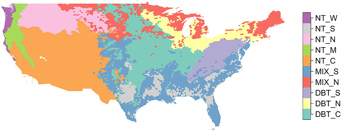
Figure 2. Map of the 10 forest strata regions used in this analysis. For each hexagon we calculated the most abundant forest PFT according to the NLCD 2019 classification map (DBT, NT, MIX), and then we further segmented these PFTs into regional strata based primarily on the level two EPA ecoregion classification map.

2.5.4. SISA model validation

Here, we explain our approach to validate the SISA models, in which validation primarily hinges on whether or not the models produced realistic footprint level distributions of AGBD. Implicit in the usage of the models at the unit level for AGBD prediction is the assumption that the models are spatially invariant—the models are unbiased at the unit level and realistically predict AGBD despite being trained at an aggregate scale. Our validation approach assesses the extent to which this assumption of scale invariance is met based on the data available. We first examined the applicability of the β parameter estimates at the unit level by comparing distributions of SISA predicted AGBD with the distributions of FIA plot level AGBD. Second, we assessed the internal consistency of the β parameter estimates and their uncertainty between the hexagon (aggregate) and footprint (unit) levels. If (1) the unit level distribution of SISA AGBD predictions matched the unit level distribution of FIA plot AGBD, and (2) $\widehat{\beta }$ appeared consistent across different spatial scales of aggregation, we determined there was not sufficient evidence to invalidate the assumption of spatial invariance, thus rendering unit level AGBD prediction via the SISA models reliable for hybrid estimation of AGBD.

The final SISA model for each forest stratum was selected to maximize the similarity in unit level AGBD distributions between the FIA plots and SISA predictions. We assumed the ability of a given SISA model to reproduce its stratum's unit level distribution of FIA plot level biomass was a reliable indicator of model performance at the unit level. Therefore, if a stratum's distribution of SISA predictions was similar to the distribution of FIA plot level AGBD, we determined the corresponding SISA model was unbiased and the predictions were realistic. We also included the L4A predictions in these distribution comparisons, allowing us to characterize each SISA model's performance, relative to that of L4A, within its stratum. For example, if the SISA distribution had obvious differences relative to the FIA distribution, but less so than the L4A distribution, we deemed the SISA model as preferable to the L4A model. We also applied the appropriate SISA model to each GEDI calibration plot based on its location, to compare model performance (L4A and SISA) directly, relative to the field estimate of AGBD (Supplementary Figures 7, 8).

To assess the internal consistency of the β parameter estimates, and by extension whether the SISA predictions were reliable at the unit level, we asked the following question: If we re-calibrated the SISA models at a different spatial scale of aggregation, would the various $\widehat{\beta }$ confidence intervals overlap? In other words, does the spatial scale of calibration impact the statistical consistency of $\widehat{\beta }$? To answer this question, we recalibrated each stratum's final SISA model (Supplementary Table 2) at three different hexagon grid resolutions, with approximate areas of 12,400, 1,770, and 250 km² (Uber, 2018). This required generating versions of our SISA prediction strata and the response and predictor variables within each new hexagon grid resolution, as follows. We mapped the prediction strata into each new hexagon grid based on which strata was most abundant within each hexagon in the new grids. For the predictor variables we aggregated the GEDI metrics within each new hexagon grid as we did for the original FIA hexagon grid. For the response variable, we recalculated the FIA-based estimates within each new grid using the Horvitz-Thompson estimator, which produced similar estimates to the post-stratified estimates of Menlove and Healey (2020), and were easier to implement and reproduce (May et al., 2023). We then refit the final SISA models for each new resolution, the result of which was a new β parameter estimate associated with the model fit for each stratum and resolution combination. The statistical consistency of each stratum's SISA model form was assessed by comparing the resultant β parameter estimates and the associated 95% confidence intervals across the different spatial scales of model calibration.

3. Results

In the following section, we present the collective SISA model performance, quantify the impact of our filtering and SISA modeling procedures on GEDI's estimation process, and compare each set of GEDI AGBD hexagon estimates (original, filtered, and fusion) to the FIA AGBD hexagon estimates. Additional figures can be found in the Supplementary material.

3.1. SISA model validation

The SISA models produced distributions of footprint level AGBD that were similar to the FIA plot level distributions for all 10 forest strata, but to varying degrees (Figure 3). Relative to the L4A unit level distributions, the SISA unit level distributions were equally or more similar to the FIA unit level distributions in all regions, based on a side-by-side visual comparison and quantile-quantile plots. When applied to GEDI calibration plots, the L4A models explained a larger fraction of the overall variance in the field-based estimate of AGBD and had a lower root mean squared error (RMSE) than the SISA models (Supplementary Figure 7). This is expected, as the L4A models were fit on these data using a least squares approach which mathematically guarantees a lower squared error compared to the SISA models that were not calibrated on these data. However, the SISA models appeared less biased than the L4A models for low (<60 Mg ha−1) and high (>500 Mg ha−1) field-based AGBD. The SISA models were biased high in the 150–250 Mg ha−1 range of field-based AGBD.

FIGURE 3

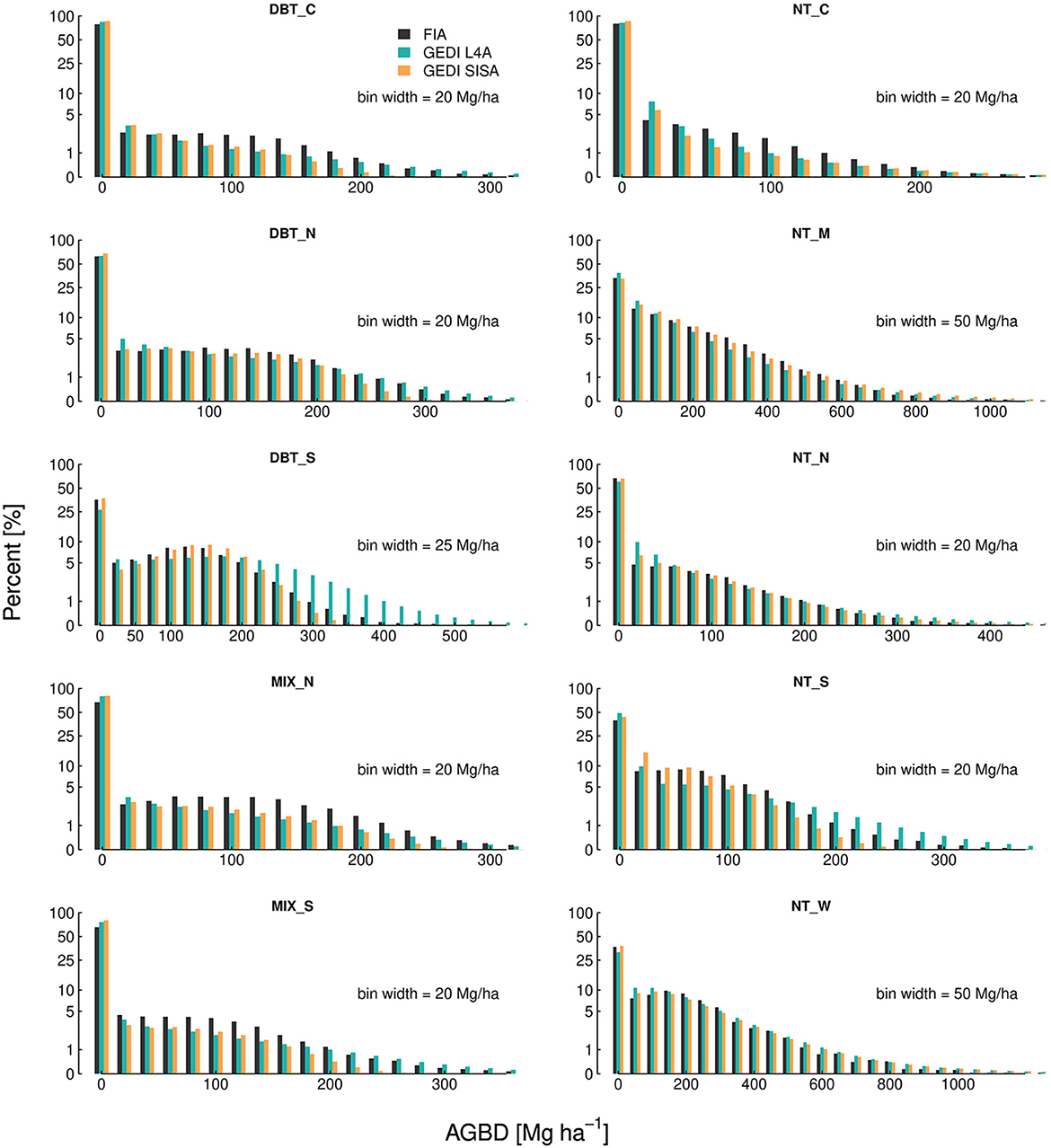
Figure 3. Unit level AGBD histograms demonstrate the SISA models generally produce realistic distributions that align with the FIA distributions, more so than the L4A distributions.

As a whole, there was moderate overlap in the SISA β parameter estimate confidence intervals across spatial scales, with some strata displaying a higher degree of consistency than others (Figure 4). The DBT_S, DBT_N, NT_N, NT_W strata exhibited relative consistency across spatial scales; these strata were more homogeneous and spatially compact relative to the other strata, individually had above average proportions of forest (Table 1), and collectively were 44.4% forested. Conversely, the parameter estimates for the DBT_C, MIX_N, NT_C strata varied across spatial scales (Figure 4), and in some instances (e.g., NT_C) the variation was large relative to the point estimates. Relative to the four strata with more stable parameter estimates, these three strata were more disjointed and ecotonal, and collectively were only 25.5% forested. The MIX_S, NT_S, NT_W strata exhibited mixed consistency in β parameter estimates across scales; these strata had characteristics in between those with consistent and inconsistent β parameter estimates and collectively were 42.8% forested.

FIGURE 4

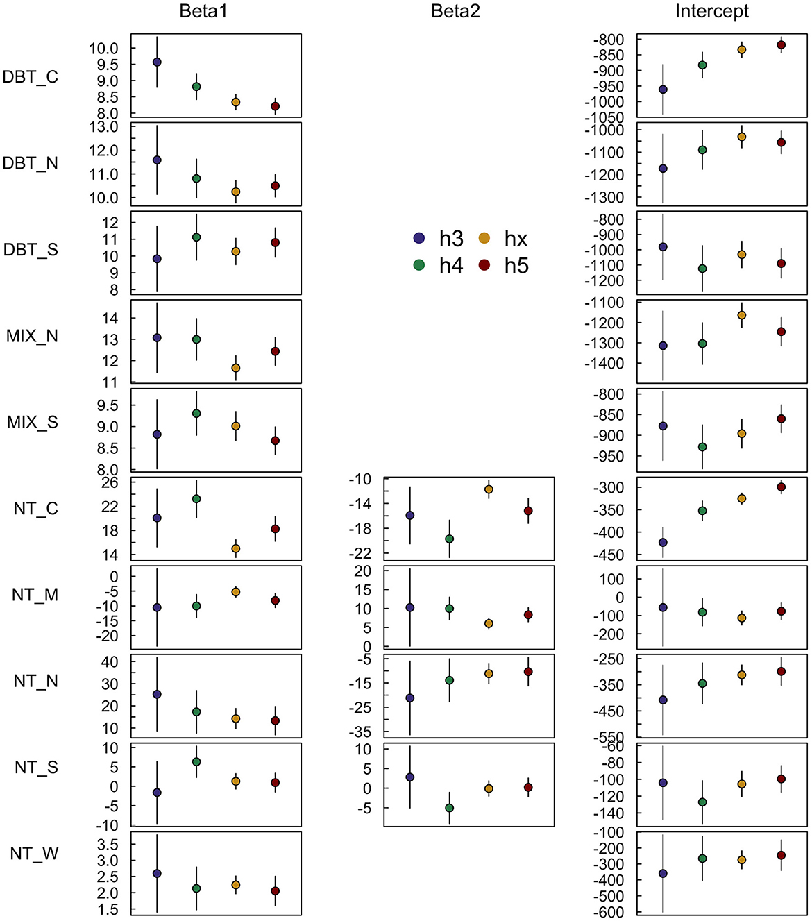
Figure 4. SISA model β parameter estimates consistent to varying degrees when calibrated at four different spatial resolutions. The h3 (~12,393 km²), h4 (~1,770 km²), and h5 (~253 km²) resolutions are different hexagon tessellations from the H3 hierarchical spatial indexing system, and the hx resolution (~640 km) is the FIA's hexagon grid used throughout this analysis. Broadly, the more homogeneous strata with high proportions of forest cover exhibited a greater degree of stability in the parameter estimates across spatial scales than strata with lower forested proportions and more forest type heterogeneity.

TABLE 1

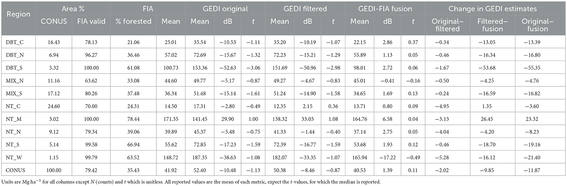
Table 1. FIA and GEDI estimates and GEDI change statistics by forest stratum and for all the continental US (COUNS).

3.2. Changes to the GEDI hexagon biomass estimates

The additional filtering criteria that we implemented had substantial impacts on GEDI's biomass estimates in certain areas, and no impact in others (Supplementary Figure 10A). The spatial pattern of differences between the original and filtered GEDI estimates shows that filtering was most helpful in the western third of the country, which is almost entirely due to the removal of topography impacted observations. The impact of cloud filtering was not nearly as concentrated nor as large, and was mostly randomly distributed throughout eastern deciduous forests. Cloud filtering resulted in the removal of 618,615 GEDI observations, or 0.11% of all observations that made it through GEDI's original quality filters.

The original GEDI estimates contained an average of 43,516 observations per intact hexagon (excludes coastal and partial hexagons with a land area less than 600 km², N = 11,631). Our filtering procedures removed an average of 59 observations per hexagon, resulting in an average decrease of 1.91 Mg ha−1 between the original and filtered GEDI estimates. However, of the 12,550 total hexagons, our filtering techniques did not remove any observations in 3,752 hexagons. Further, 14.1% of hexagons had more than 100 observations removed (resulting in a mean decrease of 8.8 Mg ha−1 between the original and filtered estimates for these 1,768 hexagons), and 0.58% of hexagons had more than 1,000 shots removed (resulting in a mean decrease of 21.94 Mg ha−1 between the original and filtered estimates for these 73 hexagons).

The SISA models resulted in an average decrease of 9.85 Mg ha−1 between the filtered and fusion estimates (Table 1), although the magnitude and direction of change varied considerably by region (Supplementary Figure 10B). The largest absolute mean change at the region level occurred in the Appalachian Mountains (DBT_S), where the SISA models resulted in an average decrease in the mean estimate of 53.68 Mg ha−1 per hexagon. The other region with a notably large change included the Cascade and Sierra Mountain ranges (NT_M), with an average increase of 26.45 Mg ha−1 per hexagon.

3.3. GEDI and FIA hexagon estimate comparisons

There were widespread and systematic differences between the original GEDI and FIA estimates (Figure 5). The GEDI map overestimated relative to FIA throughout much of the eastern deciduous forests, and underestimated in the PFT-mixed or predominantly conifer forests in Maine, much of the southwest, and Sierra and Cascade mountain ranges. The mean difference (FIA minus GEDI) across all hexagons was −10.48 Mg ha−1 (Table 1), and the RMSD was 27.99 Mg ha−1 . The median of test statistic t_original from Equation (2) was −1.13, with first and third quartiles of −2.81 and 0.24.

FIGURE 5

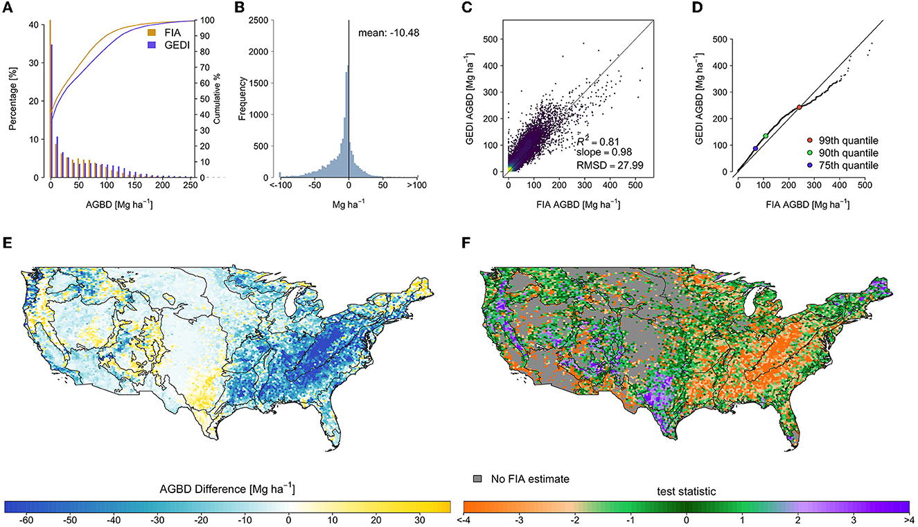
Figure 5. Hexagon-level comparison of the original GEDI estimates and FIA design-based estimates, which revealed systematic and widespread differences that are unlikely due to chance. (A) Side-by-side histogram comparison, truncated to 300 Mg ha−1 to show detail, (B) estimate difference histogram (FIA-GEDI), (C) scatter plot of FIA vs. GEDI estimates, (D) quantile-quantile plot of hexagon estimates, and maps of (E) estimate differences (FIA-GEDI), and (F) t_original, with EPA level II ecoregions overlaid.

The spatial pattern of differences between the filtered GEDI and FIA estimates was mostly similar to that of the differences between the original GEDI and FIA estimates (Figure 6), with clustered areas of improvement in the west. The mean difference improved by 2.02 to −8.46 Mg ha−1 (Table 1), and the RMSD improved slightly to 27.04 Mg ha−1 . The median of test statistic t_filtered from Equation (2) was −0.87, with first and third quartiles of −2.47 and 0.48.

FIGURE 6

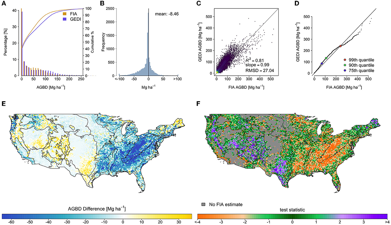
Figure 6. Hexagon-level comparison of the filtered GEDI estimates and FIA design-based estimates, in which the systematic and widespread differences between the estimates were only somewhat reduced, mainly in the west. (A) Side-by-side histogram comparison, truncated to 300 Mg ha−1 to show detail, (B) estimate difference histogram (FIA-GEDI), (C) scatter plot of FIA vs. GEDI estimates, (D) quantile-quantile plot of hexagon estimates, and maps of (E) estimate differences (FIA-GEDI), and (F) t_filtered, with EPA level II ecoregions overlaid.

The SISA models resulted in considerable improvement in the fusion estimates relative to the FIA estimates (Table 1). The spatial pattern of the differences relative to the FIA's estimates changed substantially, and while some localized patterns of systematic difference remained, the general pattern of overestimation in eastern deciduous forests and underestimation of western conifer forests was eliminated (Figure 7). The mean difference across all hexagons was 1.39 Mg ha−1 , and the RMSD was 18.10 Mg ha−1 . The median of test statistic t_fusion from Equation (2) was 0.11, with first and third quartiles of −0.88 and 0.98.

FIGURE 7

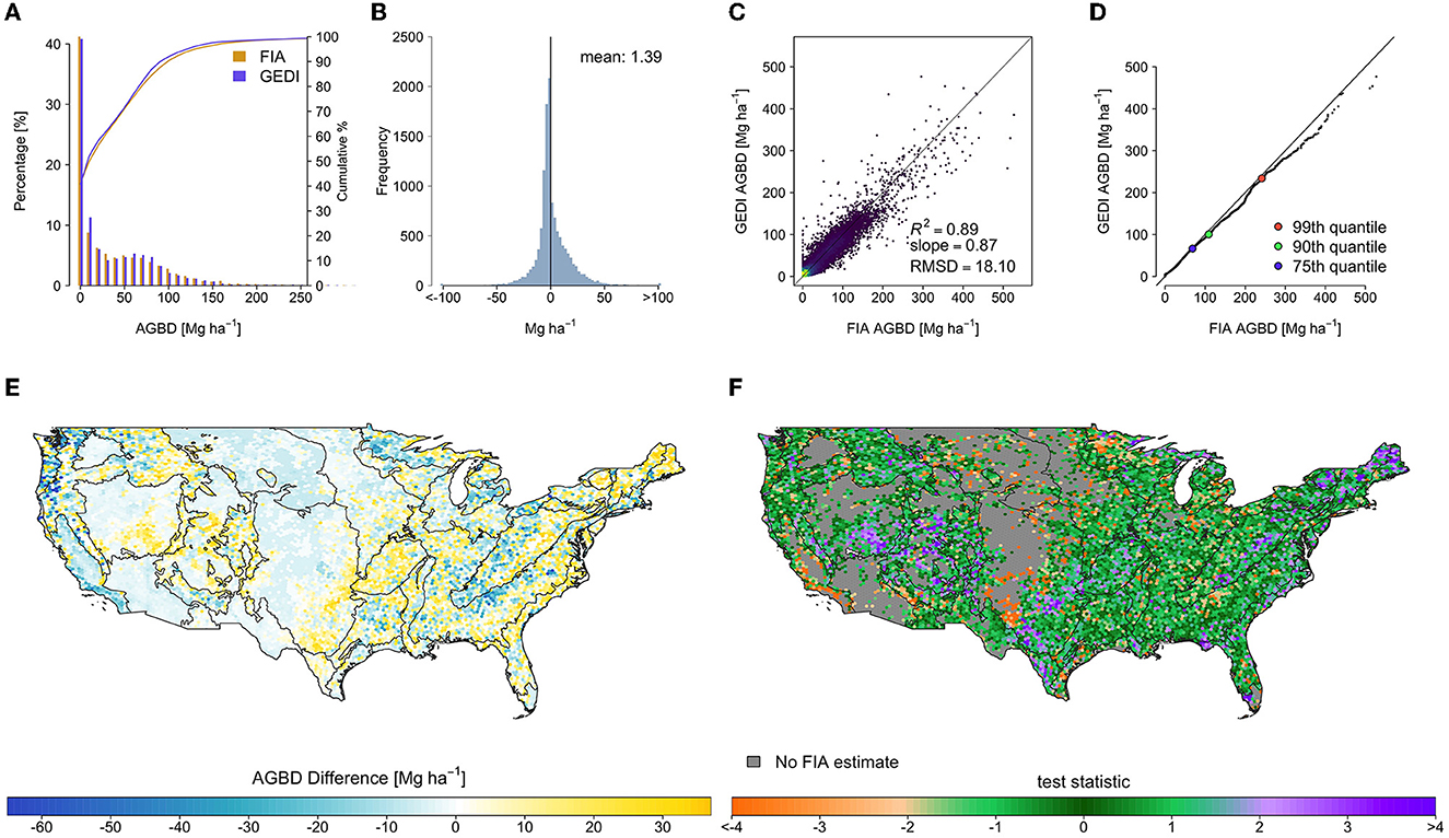
Figure 7. Hexagon-level comparison of the fusion GEDI estimates and FIA design-based estimates, in which the spatial pattern of differences between the filtered GEDI and FIA estimates were all but eliminated, indicating substantial agreement between the GEDI fusion and FIA AGBD estimates. (A) Side-by-side histogram comparison, truncated to 300 Mg ha−1 to show detail, (B) estimate difference histogram (FIA-GEDI), (C) scatter plot of FIA vs. GEDI estimates, (D) quantile-quantile plot of hexagon estimates, and maps of (E) estimate differences (FIA-GEDI), and (F) t_fusion, with EPA level II ecoregions overlaid.

In total, our improvements to GEDI's AGBD estimation process resulted in a bias reduction of 86.7%; 19.3% due to improved filtering, and the remaining 67.5% due to the SISA models. Here, we define estimate bias as the percent change between mean absolute differences in the FIA and GEDI estimates. In every strata the distribution of t_fusion was more centered on 0 than for t_filtered or t_original (Figure 8). In all strata the interquartile range t_fusion was smaller than for t_filtered or t_original with the exception of NT_W, where it was comparable. This is not a surprising result, because the SISA models were calibrated using the FIA hexagon estimates (see Section 4).

FIGURE 8

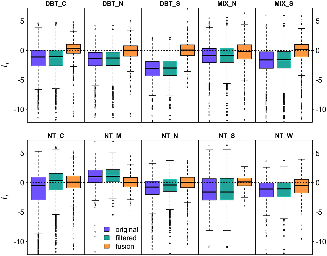
Figure 8. Boxplots of t_i from the original, filtered, and fusion estimates show that for all regions, the fusion estimates are in better agreement with the FIA estimates than the original or filtered estimates, with smaller interquartile ranges that are more centered on 0.

The standard error associated with the original and filtered estimates were similar (Figure 9), with respective mean values of 1.94 and 1.85 Mg ha−1 , compared to a mean standard error of 2.57 Mg ha−1 for the fusion estimates, and 10.88 Mg ha−1 for the FIA estimates. The respective mean standard errors as a percentage of the mean estimate were 6.0, 7.1, 12.9, and 38.1%. These reported values represent hexagons with two or more forested FIA plots (N = 9,851), because it is not possible to produce a valid standard error estimate for hexagons with fewer than 2 plots.

FIGURE 9

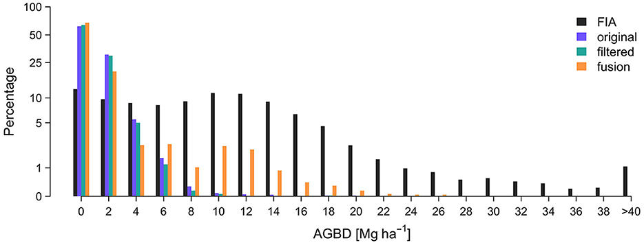
Figure 9. FIA's design-based hexagon standard error estimates are substantially larger than GEDI's hybrid standard error estimates from GEDI's original, filtered, and fusion mean estimates. The fusion hexagon standard error estimates are more likely than the filtered or original estimates to be <2 Mg ha−1 , while also displaying a multimodal response similar to that of the FIA standard errors, but to a lesser degree.

3.4. Gridded 1 km resolution fusion estimates

At the 1 km scale, mean AGBD was 45.6 Mg ha−1 from the original GEDI estimates, and 37.2 Mg ha−1 from the fusion estimates (Figure 10). For 1 km cells with mean estimates less than 100 Mg ha−1 , the respective mean standard errors were 4.5 and 4.8 Mg ha−1 , and for 1 km cells with mean estimates larger than 100 Mg ha−1 , the average standard error as a percentage of the mean estimate were 11.4 and 10.9%. Here, the difference in uncertainty reporting (Mg ha−1 vs. percentage of the mean) is to coincide with GEDI's specific precision requirements; estimate precision for grid cells with a mean estimate below 100 Mg ha−1 should be reported in units of Mg ha−1 , while estimate precision for grid cells with a mean estimate greater than or equal to 100 Mg ha−1 should be reported as a percentage of the mean estimate.

FIGURE 10

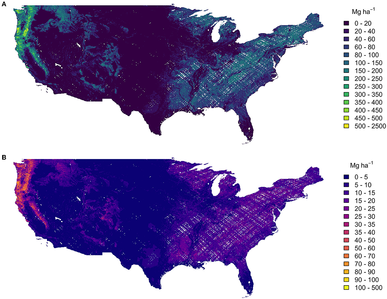
Figure 10. Mean 1 km estimates of AGBD (A) and its uncertainty (B). The white areas in both maps are gaps in the GEDI sample at 1 km scale.

4. Discussion

The GEDI mission represents an advance in global biomass mapping, because the ability to characterize estimate uncertainty and flag deviations from reference estimates that are unlikely due to chance allows for iterative improvements to GEDI's overall estimation process (Dubayah et al., 2022b). We leveraged this ability to identify and mitigate the filtering and L4A model misspecification issues that adversely impacted GEDI's estimation process. In the discussion that follows we first summarize why stricter data filtering is important and should be implemented with care. We present a possible cause of L4A model bias in certain regions within the US, and explain how the SISA framework accommodates this phenomena. We then acknowledge the shortcomings in our SISA modeling approach, specifically how modeling assumptions may be violated to varying degrees in certain areas, and the implications for the resultant predictions and estimates. We conclude with comments on the circularity of comparing the fusion GEDI and FIA references estimates in a probabilistic manner.

GEDI's data filtering procedure applies a set of rules to identify waveforms not suited for biomass estimation (Healey et al., 2022). Our findings suggest that additional filtering of a small number of observations impacted by topography or low clouds can improve GEDI's biomass estimates at the hexagon scale, and by extension, other spatial scales. However, caution must be exercised when identifying such observations so as not to violate the hybrid assumption of a random cluster sample. We did not implement any additions to the AGBD estimation process to deal with an increased number of non-response samples relative to GEDI's original estimates, for two reasons. First, we needed to implement the exact estimation method used to produce the original GEDI estimates to ensure a like-comparison of results. Second, the number of observations designated as non-response by our added filtering practices was very small relative to the number of GEDI observations already removed from the sample by GEDI's current filtering procedures. Our topographic filtering approach removes a small number of GEDI observations heavily impacted by topography, deceasing AGBD estimation bias without substantially impacting the GEDI sample. Reducing the impact of clouds and fog within 150 m of the land surface globally is more challenging, especially when clouds and fog can occur below the height of the tallest tree in an area. Our cloud filtering approach is straightforward and only removes affected observations with heights larger than the tallest trees. In future studies we recommend development of algorithms to improve detection of low clouds and fog impacting GEDI waveforms.

Availability of calibration data is a limiting factor to unbiased, continental scale biomass mapping with GEDI. The spatial pattern of differences between the filtered GEDI and FIA estimates (Figures 6E, F) implies a systematic issue somewhere else in the AGBD estimation process that is not related to data filtering. Despite the considerable effort spent to ensure a representative L4A training sample and unbiased models (Duncanson L. et al., 2022), the attenuation of this spatial pattern in the differences between the fusion GEDI and FIA estimates (Figures 7E, F) suggests that L4A model bias is the primary cause.

The results for MIX_N and NT_N are especially informative, given these strata respectively contained 85.3 and 67.9% of the calibration plots used to train the L4A DBT and NT models (Supplementary Table 3). In both strata the L4A models appear unbiased, as the unit level distributions are similar to those from the FIA (Figure 3), and there are not widespread systematic differences between the filtered GEDI and FIA hexagon level AGBD estimates (Figures 7E, F, 8). Conversely in other strata, there is substantial disagreement in between the L4A and FIA unit level distributions and the filtered and FIA hexagon estimates. Two such strata are DBT_S and NT_M, which respectively contain 0.4 and 4.5% of the GEDI calibration plots for the L4A DBT and NT models (Supplementary Table 3). As geographic transferability was prioritized during the L4A model calibration process, these specific L4A models had the best performance when applied to validation data outside of the geographic extent of training data, relative to all the candidate models tested during L4A calibration (Duncanson L. et al., 2022). In other words, the L4A models are as unbiased as possible given the available training data. Yet, substantial discrepancies in observed L4A performance exist across space; the observation that the L4A models appear better specified in MIX_N and NT_N than in DBT_S and NT_M allows for the possibility that the relationship between forest structure and AGBD varies spatially. Variation in the relationship between forest structure and AGBD between the DBT_S and MIX_N strata, and between the NT_M and NT_N strata, could explain the difference in L4A model performance, because the training data are more representative of the MIX_N and NT_N strata than of the DBT_S and NT_M strata. That the L4A and FIA unit level distributions and the filtered GEDI and FIA estimates match at all in some regions despite spatially varying relationships and limited training data is a testament to the L4A calibration and validation process.

The SISA modeling framework accounts for spatial variation in the relationship between GEDI derived forest structure metrics and AGBD in two ways. First, model development at the aggregate (hexagon) scale ensured training data with uniform spatial coverage throughout each of the 10 prediction strata, appropriately capturing within-strata variability in the structure to biomass relationship. Second, the large number of hexagons within the US allowed for more localized and homogeneous prediction strata relative to L4A's two continental scale prediction strata. The SISA prediction strata contain presumably less variation in the local structure to biomass relationships than the continental scale DBT and NT L4A strata, thus decreasing the likelihood of localized model bias within a SISA stratum. Our comparisons of the SISA, L4A, and FIA unit level distributions of AGBD demonstrate the importance of accounting for spatial variability in forest structure and biomass. For all strata, the SISA distributions were equally or more realistic than the L4A distributions, which leads us to conclude that as a whole the SISA models produced more accurate and realistic predictions than the L4A models. This was most apparent in the DBT_S and NT_M strata, where the application of the SISA models resulted in marked improvement over the L4A models, for both the unit level distributions (Figure 3) and the hexagon estimate comparisons (Figure 7). The SISA models for DBT_N, DBT_S, NT_N, NT_M, NT_W appeared definitively unbiased. In DBT_C and NT_C the SISA and FIA distributions were marginally different above approximately 50 Mg ha−1 , with SISA biased low relative to FIA, implying a low to moderate level of bias in these strata. In contrast, larger differences between the SISA and FIA unit level distributions in MIX_N, MIX_S, and NT_S suggested the SISA models are likely biased to a greater extent in these strata.

Instances of SISA model bias presupposes that the assumption of SISA model spatial invariance has not been met in these areas. The SISA model derivation in Section 2.5.2 provides a theoretical justification for the assumption of scale invariance necessary for prediction at the unit level, which we then evaluated using the available in situ data following our validation scheme in Section 2.5.4. The unit level distributions, used here as a method of evaluating the extent to which the SISA models may be biased or not, suggest that the SISA models are mostly unbiased, but that some areas of moderate to substantial model bias are probable. This interpretation is supported by the analysis of SISA model parameter estimates across spatial scales. While an overlap of confidence intervals does not guarantee equality in the parameter estimates by itself, it is another manner by which we evaluate the assumption of spatial invariance, in combination with unit level distribution comparisons. The overlap of confidence intervals in the DBT_N, DBT_S, NT_M, NT_N, NT_W strata, along with the matching FIA and SISA unit level distributions, suggests a lack evidence sufficient for invalidation of the assumption of scale invariance in these strata. However, parameter estimates for which the confidence intervals do not overlap across spatial scales within a strata is sufficient evidence of invalidation of this assumption, especially when sample sizes are large. Thus the observed scale-dependent variability in the parameter estimates for DBT_C, NT_C, MIX_N, MIX_S supports the results from the unit level distributions, that the assumption of scale invariance in these strata is not met to the same degree as in other strata.

Degradation of scale invariance leading to SISA model bias in certain regions leads us to believe that, despite our best efforts, one or both of the assumptions underpinning our SISA model derivation were violated to some degree in certain areas. There are several mechanisms by which these assumptions—a consistent relationship between predictor and response variables that is linear at both the aggregate and unit level—could be impacted. The first is that within strata variations to the relationship between FIA AGBD estimates and forest structure quantified by GEDI would violate the assumption of a consistent relationship. This is likely true to some extent within several strata, as seen in the remaining differences between the FIA and fusion estimates within the MIX_N region (Figure 7). Relative to the FIA estimates, the fusion estimates are systematically larger in the northern mid-west, and systematically smaller throughout much of the northeast. The relationship between FIA biomass and GEDI forest structure variables to may vary longitudinally within this stratum, and as a result positive model bias in the northern midwest leads to overestimation of AGBD, while negative model bias in the northeast leads to underestimation. The decision of 10 strata was somewhat arbitrary, and future work could employ a more data driven stratification, such as Scarth et al. (2019), aimed at maximizing within-strata structural and biomass characteristics.

Similarly, a non-linear relationship between predictor and response variables at the unit level would also violate the SISA model assumption. We used all available plot level data to ensure only linear, unit level relationships were tested during SISA model calibration (Section 2.5.3, Supplementary Section 3, and Supplementary Figures 2–4). However, as the GEDI calibration plots are spatially clustered and represent some SISA strata far better than others, we may have chosen SISA relationships for which the linearity constraint breaks down in certain areas that are not well-represented by the plot level data.

A third mechanism by which the SISA model assumptions could be violated relates to a small but important difference in the population of interest between the FIA and GEDI. While GEDI does not make a distinction between forested and non-forested areas in biomass estimation, the FIA only estimates biomass within forested lands and explicitly ignores vegetation located on lands that do not meet its definition of forest. A mismatch between GEDI predictor variables used in SISA calibration that reflect non-forested vegetation and the FIA AGBD response variable that ignores such vegetation would at best add noise to a calibration data set that would not otherwise be present, and at worse could violate both the linearity and consistency assumptions within a strata or part of a strata. The strata where the SISA models appear partially biased (DBT_C, NT_C, MIX_N, MIX_S) contain some of the lowest proportions of FIA estimated forest cover of all strata (Table 1) and thus have more opportunity for non-forested vegetation to be captured by GEDI.

The comparison of the fusion GEDI hexagon estimates and the FIA hexagon estimates is circular in that the FIA reference estimates were used to calibrate the SISA models, which underpin the fusion estimates. Thus it is not surprising that the fusion estimates were in far better agreement with the FIA estimates than either the original or filtered GEDI estimates. The more interesting result was that the SISA models produced mostly realistic distributions of unit level AGBD, matching the FIA unit level distributions of AGBD. Since the SISA models were mostly unbiased and yielded realistic predictions, it follows that the fusion and reference estimates are in relative agreement. The hexagon level comparison of the fusion and reference estimates was only necessary to demonstrate that the SISA models result in mostly unbiased estimates when applied within hybrid inference. The ability to calibrate unit level models at an aggregated scale is important because it helps overcome challenges in obtaining representative training data for remote sensing based models of AGBD. Further, the fusion hexagon estimates are more precise than the FIA reference estimates (Figure 9), which reduces overall uncertainty in the US forest carbon stock and may help constrain future fluxes. This work represents not only a refinement of GEDI's biomass estimation process, but also an advance in remote sensing based methods of biophysical inference.

Data availability statement

The raw data supporting the conclusions of this article will be made available by the authors, without undue reservation.

Author contributions

JB, PM, and RD contributed to the conception and design of the study. JB, PM, and JA developed the methodology and software. JB managed the data, performed the data processing and statistical analysis, wrote the original draft of the manuscript, and lead the manuscript revisions. RD provided supervision and funding acquisition. All authors contributed to revision and editing of the original submitted version and revisions.

Funding

This work was supported by funding from the Global Ecosystem Dynamics Investigation (NASA contract NNL15AA03C) and NASA FINESST Grant (80NSSC21K1626).

Acknowledgments

The authors thank Zhiqiang Yang for assistance with the FIA database.

Conflict of interest

The authors declare that the research was conducted in the absence of any commercial or financial relationships that could be construed as a potential conflict of interest.

Publisher's note

All claims expressed in this article are solely those of the authors and do not necessarily represent those of their affiliated organizations, or those of the publisher, the editors and the reviewers. Any product that may be evaluated in this article, or claim that may be made by its manufacturer, is not guaranteed or endorsed by the publisher.

Supplementary material

The Supplementary Material for this article can be found online at: https://www.frontiersin.org/articles/10.3389/ffgc.2023.1149153/full#supplementary-material

References

Avitabile, V., Herold, M., Heuvelink, G. B., Lewis, S. L., Phillips, O. L., Asner, G. P., et al. (2016). An integrated pan-tropical biomass map using multiple reference datasets. Glob. Change Biol. 22, 1406–1420. doi: 10.1111/gcb.13139

PubMed Abstract | CrossRef Full Text | Google Scholar

Babcock, C., Finley, A. O., Andersen, H.-E., Pattison, R., Cook, B. D., Morton, D. C., et al. (2018). Geostatistical estimation of forest biomass in interior alaska combining landsat-derived tree cover, sampled airborne lidar and field observations. Remote Sens. Environ. 212, 212–230. doi: 10.1016/j.rse.2018.04.044

CrossRef Full Text | Google Scholar

Babcock, C., Finley, A. O., Bradford, J. B., Kolka, R., Birdsey, R., and Ryan, M. G. (2015). Lidar based prediction of forest biomass using hierarchical models with spatially varying coefficients. Remote Sens. Environ. 169, 113–127. doi: 10.1016/j.rse.2015.07.028

CrossRef Full Text | Google Scholar

Babcock, C., Finley, A. O., Cook, B. D., Weiskittel, A., and Woodall, C. W. (2016). Modeling forest biomass and growth: coupling long-term inventory and lidar data. Remote Sens. Environ. 182, 1–12. doi: 10.1016/j.rse.2016.04.014

CrossRef Full Text | Google Scholar

Bechtold, W. A., and Patterson, P. L. (2005). The Enhanced Forest Inventory and Analysis Program–National Sampling Design and Estimation Procedures. Asheville, NC: USDA Forest Service, Southern Research Station. p. 80.

Google Scholar

Chen, X., Disney, M., Lewis, P., Armston, J., Han, J., and Li, J. (2014). Sensitivity of direct canopy gap fraction retrieval from airborne waveform lidar to topography and survey characteristics. Remote Sens. Environ. 143, 15–25. doi: 10.1016/j.rse.2013.12.010

CrossRef Full Text | Google Scholar

Dubayah, R., Armston, J., Healey, S. P., Bruening, J. M., Patterson, P. L., Kellner, J. R., et al. (2022b). GEDI launches a new era of biomass inference from space. Environ. Res. Lett. 17, 095001. doi: 10.1088/1748-9326/ac8694

CrossRef Full Text | Google Scholar

Dubayah, R., Armston, J., Healey, S., Yang, Z., Patterson, P., Saarela, S., et al. (2022a). GEDI l4b Gridded Aboveground Biomass Density, version 2.

Google Scholar

Dubayah, R., Armston, J., Kellner, J., Duncanson, L., Healey, S., Patterson, P., et al. (2021). GEDI l4a Footprint Level Aboveground Biomass Density, version 2. ORNL DAAC, Oak Ridge, TN.

Google Scholar

Dubayah, R., Blair, J. B., Goetz, S., Fatoyinbo, L., Hansen, M., Healey, S., et al. (2020). The global ecosystem dynamics investigation: high-resolution laser ranging of the Earth's forests and topography. Sci. Remote Sens. 1, 100002. doi: 10.1016/j.srs.2020.100002

CrossRef Full Text | Google Scholar

Dubayah, S., Hofton, M., Blair, J., Armston, J., Tang, H., and Luthcke, S. (2020). GEDI l2a Elevation and Height Metrics Data Global Footprint Level V001. NASA EOSDIS Land Processes DAAC.

Google Scholar

Duncanson, L., Armston, J., Disney, M., Avitabile, V., Barbier, N., Calders, K., et al. (2021). Aboveground Woody Biomass Product Validation Good Practices Protocol. doi: 10.5067/doc/ceoswgcv/lpv/agb.001

CrossRef Full Text | Google Scholar

Duncanson, L., Kellner, J. R., Armston, J., Dubayah, R., Minor, D. M., Hancock, S., et al. (2022). Aboveground biomass density models for NASA's global ecosystem dynamics investigation (GEDI) lidar mission. Remote Sens. Environ. 270, 112845. doi: 10.1016/j.rse.2021.112845

CrossRef Full Text | Google Scholar

Fay, R. E., and Herriot, R. A. (1979). Estimates of income for small places: an application of James-Stein procedures to census data. J. Am. Stat. Assoc. 74, 269–277.

Google Scholar

Friedl, M., Gray, J., and Sulla-Menashe, D. (2019). MCD12Q2 Modis/Terra+ Aqua Land Cover Dynamics Yearly l3 Global 500m Sin Grid v006. NASA EOSDIS Land Processes DAAC.

Google Scholar

Fuller, W. A. (2009). Measurement Error Models. New York, NY: John Wiley & Sons.

Google Scholar

Healey, S. P., Patterson, P. L., Saatchi, S., Lefsky, M. A., Lister, A. J., and Freeman, E. A. (2012). A sample design for globally consistent biomass estimation using lidar data from the geoscience laser altimeter system (GLAS). Carbon Balance Manage. 7, 1–9. doi: 10.1186/1750-0680-7-10

PubMed Abstract | CrossRef Full Text | Google Scholar

Healey, S. P., Patterson, P. L., and Armston, J. (2022). Algorithm Theoretical Basis Document (atbd) for Gedi Level-4b (l4b) Gridded Aboveground Biomass Density. College Park, MD: University of Maryland.

Google Scholar

Hofton, M., Blair, J. B., Story, S., and Yi, D. (2020). Algorithm Theoretical Basis Document (atbd) for Gedi Transmit and Receive Waveform Processing for l1 and l2 Products. College Park, MD: University of Maryland.

Google Scholar

Hoppus, M., and Lister, A. (2007). “The status of accurately locating forest inventory and analysis plots using the global positioning system,” in Proceedings of the Seventh Annual Forest Inventory and Analysis Symposium (Washington, DC: US Department of Agriculture, Forest Service), 179–184.

Google Scholar

Kellner, J., Armston, J., and Duncanson, L. (2022). Algorithm theoretical basis document for GEDI footprint aboveground biomass density. Earth Space Sci. 10, e2022EA002516. doi: 10.1029/2022EA002516

CrossRef Full Text | Google Scholar

Margolis, H. A., Nelson, R. F., Montesano, P. M., Beaudoin, A., Sun, G., Andersen, H.-E., et al. (2015). Combining satellite lidar, airborne lidar, and ground plots to estimate the amount and distribution of aboveground biomass in the boreal forest of North America. Can. J. Forest Res. 45, 838–855. doi: 10.1139/cjfr-2015-0006

CrossRef Full Text | Google Scholar

May, P., McConville, K. S., Moisen, G. G., Bruening, J., and Dubayah, R. (2023). A spatially varying model for small area estimates of biomass density across the contiguous united states. Remote Sens. Environ. 286, 113420. doi: 10.1016/j.rse.2022.113420

CrossRef Full Text | Google Scholar

McRoberts, R. E., Næsset, E., Saatchi, S., Liknes, G. C., Walters, B. F., and Chen, Q. (2019). Local validation of global biomass maps. Int. J. Appl. Earth Observ. Geoinform. 83, 101931. doi: 10.1016/j.jag.2019.101931

CrossRef Full Text | Google Scholar

Menlove, J., and Healey, S. P. (2020). A comprehensive forest biomass dataset for the USA allows customized validation of remotely sensed biomass estimates. Remote Sens. 12, 4141. doi: 10.3390/rs12244141

CrossRef Full Text | Google Scholar

Molina, I., and Marhuenda, Y. (2015). sae: an R package for small area estimation. R J. 7, 81. doi: 10.32614/RJ-2015-007

CrossRef Full Text | Google Scholar

Nelson, R., Margolis, H., Montesano, P., Sun, G., Cook, B., Corp, L., et al. (2017). Lidar-based estimates of aboveground biomass in the continental US and Mexico using ground, airborne, and satellite observations. Remote Sens. Environ. 188, 127–140. doi: 10.1016/j.rse.2016.10.038

CrossRef Full Text | Google Scholar

Park, T., Kennedy, R. E., Choi, S., Wu, J., Lefsky, M. A., Bi, J., et al. (2014). Application of physically-based slope correction for maximum forest canopy height estimation using waveform lidar across different footprint sizes and locations: tests on LVIS and GLAS. Remote Sens. 6, 6566–6586. doi: 10.3390/rs6076566

CrossRef Full Text | Google Scholar

Patterson, P. L., Healey, S. P., Ståhl, G., Saarela, S., Holm, S., Andersen, H.-E., et al. (2019). Statistical properties of hybrid estimators proposed for GEDI—NASA's global ecosystem dynamics investigation. Environ. Res. Lett. 14, 065007. doi: 10.1088/1748-9326/ab18df

CrossRef Full Text | Google Scholar

Pratesi, M., and Salvati, N. (2008). Small area estimation: The eblup estimator based on spatially correlated random area effects. Statist. Meth. Appl. 17, 113–141. doi: 10.1007/s10260-007-0061-9

CrossRef Full Text | Google Scholar

Pugh, S. A., Turner, J. A., Burrill, E. A., and David, W. (2018). The Forest Inventory and Analysis Database: Population Estimation User Guide. USDA Forest Service, Washington, DC.

Google Scholar

Rao, J. N., and Molina, I. (2015). Small Area Estimation. New York, NY: John Wiley & Sons.

Google Scholar

Saatchi, S. S., Harris, N. L., Brown, S., Lefsky, M., Mitchard, E. T., Salas, W., et al. (2011). Benchmark map of forest carbon stocks in tropical regions across three continents. Proc. Natl. Acad. Sci. U.S.A. 108, 9899–9904. doi: 10.1073/pnas.1019576108

PubMed Abstract | CrossRef Full Text | Google Scholar

Santoro, M., and Cartus, O. (2021). Global Datasets of Forest Above-Ground Biomass for the Years 2010, 2017 and 2018, v2. Centre for Environmental Data Analysis 10.

Google Scholar

Scarth, P., Armston, J., Lucas, R., and Bunting, P. (2019). A structural classification of Australian vegetation using ICESAT/GLAS, ALOS PALSAR, and LANDSAT sensor data. Remote Sens. 11, 147. doi: 10.3390/rs11020147

CrossRef Full Text | Google Scholar

Taylor-Rodriguez, D., Finley, A. O., Datta, A., Babcock, C., Andersen, H.-E., Cook, B. D., et al. (2019). Spatial factor models for high-dimensional and large spatial data: an application in forest variable mapping. Stat. Sin. 29, 1155. doi: 10.5705/ss.202018.0005

PubMed Abstract | CrossRef Full Text | Google Scholar

Uber, H. (2018). Hexagonal hierarchical geospatial indexing system.

Google Scholar

Yang, W., Ni-Meister, W., and Lee, S. (2011). Assessment of the impacts of surface topography, off-nadir pointing and vegetation structure on vegetation lidar waveforms using an extended geometric optical and radiative transfer model. Remote Sens. Environ. 115, 2810–2822. doi: 10.1016/j.rse.2010.02.021

CrossRef Full Text | Google Scholar