Monitoring and mapping vegetation greenery in residential communities using street view images and a Normalized Vegetation Greenery Index: a case study in Beijing, China

Vegetation greenery is essential for the sensory and psychological wellbeing of residents in residential communities. To enhance the quality of regulations and policies to improve people’s living environments, it is crucial to effectively identify and monitor vegetation greenery from the perspective of the residents using effective images and methods. In this study, Baidu street view (BSV) images and a Normalized Vegetation Greenery Index (NVGI) based method were examined to distinguish vegetation greenery in residential communities of Beijing, China. The magnitude of the vegetation was quantified and graded, and spatial analysis techniques were employed to investigate the spatial characteristics of vegetation greenery. The results demonstrated that (1) the identified vegetation greenery using the proposed NVGI-based method was closely correlated with those of the reference classification (r = 0.993, p = 0.000), surpassing the comparison results from the SVM method, a conventional remote sensing classification means; (2) the vegetation greenery was distributed unevenly in residential communities and can be categorized into four grades, 63.79% of the sampling sites were found with relatively low (Grade II) and moderate (Grade III) vegetation greenery distribution, most of the districts in the study area contained zero-value green view index sites; and (3) there was significant spatial heterogeneity observed in the study area, with low-value clustering (cold spots) predominantly located in the central region and high-value clustering (hot spots) primarily concentrated in the peripheral zone. The findings of this study can be applied in other cities and countries that have street view images available to investigate greenery patterns within residential areas, which can help improve the planning and managing efforts in urban communities.

1. Introduction

The vegetation greenery in residential communities, such as arbor trees, shrubs, bamboos, and lawns, has favorable effects on residents’ sensory and psychological wellbeing (Wolch et al., 2014; Engemann et al., 2019; Wu et al., 2021; Ma et al., 2022). However, greenery in residential areas is more likely to be removed or destroyed as a result of private appropriation. The green vegetation in residential communities should be classified and monitored using an appropriate profile dataset and classification methodology, enabling planners to utilize the information as a guide for developing more specialized planning and management strategies. However, few studies have focused on identifying the spatial heterogeneity of vegetation greenery in residential communities.

Satellite-based multi-spectral remote sensing images can cover large-scale regions and be used to fulfill canopy extraction and greenery estimations (Cai et al., 2019; Wei et al., 2020). While most of these images are acquired from the aerial perspective, the greenery computed using the satellite remote sensing images reflects the characteristics and situation of the canopy from the top to the bottom, which may different from residents’ common view of greenery observed at ground. Additionally, commonly used multi-spectral remote sensing images are acquired through passive detecting technology, which is subjective to the influences of clouds, precipitation, haze, and green vegetation thickness (Woodhouse, 2017).

Profile imaging systems, such as Google street view, Tencent street view, and Baidu street view (BSV), have similar view angles to residents, and they can present the greenery environment at a very high-resolution level (Gu et al., 2019; Liu et al., 2020; Li et al., 2021). As a result, the street view images can be used to map and quantify the amount of street-side greenery. For instance, Yang et al. (2009) developed a green view index based on Google street view images to evaluate the visibility of urban forests in Berkley, California, USA. Griew et al. (2013) developed and tested a street audit tool using Google street view in Wigan, England to measure environmental supportiveness for physical activity, and found that Google street view images are reliable to be used to measure the urban street greenery. Li et al. (2015) used Google street view images to assess urban greenery in New York City, and proposed a green view index to measure the street-side greenery that people can see when standing or walking on the street; Ye et al. (2019) measured the daily accessed street greenery in Singapore using the Google street view images and deep learning method to achieve an accurate measurement on visible greenery. In China, as an alternative to Google street view, the BSV dataset is free to download using the Baidu API. It has a broader coverage and contains more up-to-date images than other profile datasets. BSV imagery is so far available in 424 China’s cities with a total distance of more than 3 million kilometers (Baidu, 2020), which has been used to effectively quantify and monitor the street-side greenery supportiveness in the metropolis, such as Shanghai (Xiao et al., 2020), Shenzhen (Zhong et al., 2021), Chongqing (Deng et al., 2021), Sanya (Chen et al., 2019), Tai’an (Yu et al., 2019), Harbin, and Changchun (Xiao et al., 2021). Therefore, the BSV image system is predicted to be a valuable source of information for precisely detecting and evaluating vegetation greenery from people’s perspectives. However, the use of the BSV imaging system to study the vegetation characteristics in enclosed spaces, especially residential communities, has not been involved.

Compared to satellite remote sensing images, street view images only provide spectral information in the red (R), green (G), and blue (B) bands (Toaha et al., 2020). Due to the absence of near-infrared (NIR) data, conventional algorithms used for remote sensing image classification are prone to misclassifying vegetation as other urban landscape elements such as buildings, vehicles, and shade (Li et al., 2019; Kumar et al., 2020), which can negatively impact the accuracy of green vegetation extraction and evaluation (Yu and Qi, 2021; Yu et al., 2022). An effective method for identifying vegetation greenery is requisite to address this issue. Additionally, the monitoring of vegetation greenery involves processing a large amount of data due to the impact of road alignment on residents’ visual ranges, requiring thousands of images to be processed. The same characteristics in images may exhibit different values for image elements due to variation in weather condition during image capture, such as cloudy and sunny days. Therefore, it is imperative to investigate methods for minimizing the difference between green vegetation and other features in BSV images, enabling effective extraction during image batch processing. Additionally, maximizing the contrast of image element values between greenery and other features should also be explored.

This study aimed to investigate the potential of BSV images and a Normalized Vegetation Greenery Index (NVGI)-based method as the source of information for identifying and evaluating vegetation greenery in residential communities, as well as exploring its spatial characteristics. Sampling sites were randomly created in the residential communities, BSV images were acquired from the sampling sites, and the proposed method was used to identify green vegetation in these images and examine its feasibility in the BSV image classification. The vegetation greenery index was computed to measure the magnitude of vegetation greenery in the residential communities and compare their spatial characteristics. The findings of this study are expected to be a reference for residential community greenery estimation and planning.

2. Study area

Beijing (115.7–117.4° E and 39.4–41.6° N) is the capital of China, it contains sixteen districts, i.e., Changping District (CP hereinafter), Chaoyang District (CY), Dongcheng District (DC), Daxing District (DX), Fangshan District (FS), Fengtai District (FT), Haidian District (HD), Huairou District (HR), Mentougou District (MTG), Miyun District (MY), Pinggu District (PG), Shijingshan District (SJS), Shunyi District (SY), Tongzhou District (TZ), Xicheng District (XC), and Yanqing District (YQ), with a total area of 16,396.54 km² (Figure 1). According to the seventh census of China, the study area had ∼22 million residents through the end of 2021, which ranked seventh around the world. Such a large population size makes it an ideal area for green vegetation identification in residential communities.

FIGURE 1

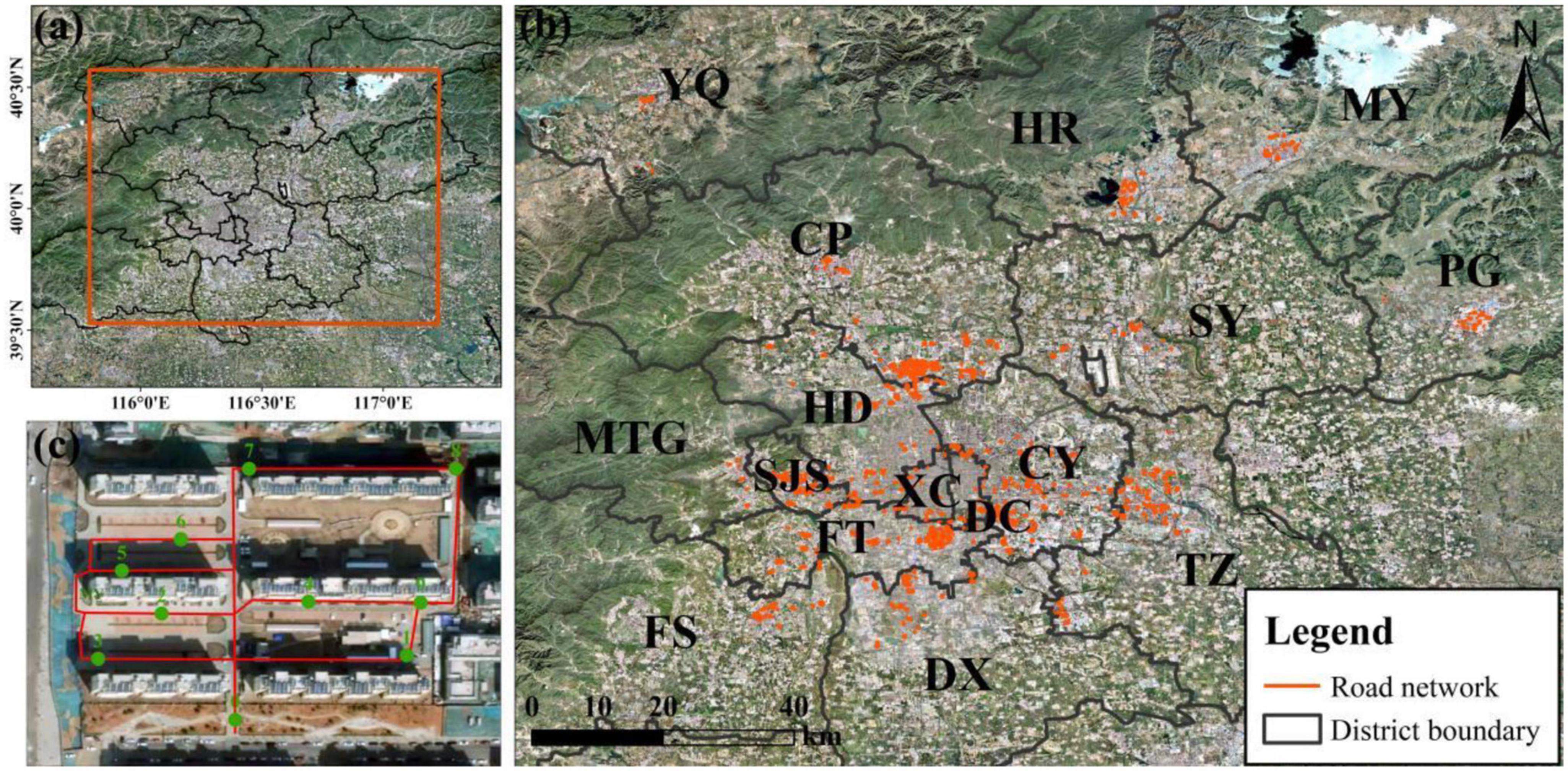
Figure 1. Study area in Beijing. (a) Location of the study area; (b) 16 districts in the study area, the red lines are the road networks in each district; (c) an example of a residential community, the red lines represent the roads in the community, and the leaf green dots represent the locations of sampling sites to obtain BSV images.

3. Materials and methods

3.1. BSV image acquisition

Due to the varying names of residential communities and the absence of applicable programming rules for extracting residential community areas, all the residential communities covered with BSV images in the study area were identified manually, and so were their inner road networks. A total length of 79.40 km road network was delineated in the study communities using the professional geographical information system software ArcGIS Desktop^® 10.1 (Environmental Systems Research Institute, Inc., Redlands, CA, USA). Considering the visible distance in the residential community, a minimum distance of 100 m was established between two adjacent sampling sites. A total of 7,940 sampling sites were thus randomly selected throughout the road networks. Subsequently, these sites were thoroughly examined and 245 candidates that were situated too close to other sites at the intersections were eliminated. Finally, a total of 7,695 sampling sites were selected and assigned sequential BSV-ID (0-7694) for investigation and analysis (Table 1). It should be noted that “greenery” is constantly used in this study to characterize the amount of green vegetation and to differentiate it from the “greenness” of the tasseled cap transition in remote sensing processing method.

TABLE 1

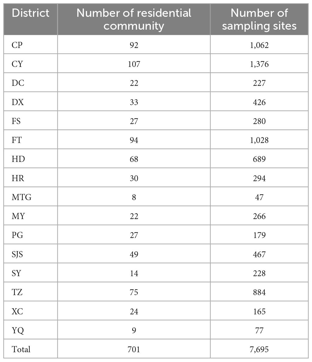
Table 1. Distribution of sampling sites in the study area.

To reduce the impact of fluctuations in road width on the assessment, this study used BSV images that were taken along the road direction. For instance, all the sampling sites distributed along the north-south (N-S) oriented roads would have BSV images heading northwards; BSV images facing east were chosen and acquired for the roads with an east-west orientation (E-W). Each available BSV image can be requested in an HTTP URL form using BSV Image API.¹ In this study, the obtained BSV images have a 160° horizontal coverage and 0° vertical coverage, which is similar to people’s optic angle and view.

3.2. Image classification and comparison with a conventional method

Similar to other profile image systems, BSV imagery includes no NIR information but captures only R, G, and B band information. The spectral ranges of landscape features in the residential community, including sky, shade, pole, vehicle, building, and pavement, largely overlap with each other’s, which makes the images less useful as the source of information for vegetation classification. Thus, image classification methods that employ NIR band information or NIR-based vegetation indices may not be able to effectively identify vegetation in BSV images and distinguish vegetation from other artificial features.

This study compared the various combinations of the three band information (Table 2). The information of R, G, and B, and the sum, subtract, and divide of these three bands were computed respectively. The R, G, and B band values were normalized using Equation 1 to minimize the pixel value difference of the same commonly seen features. The value ranges of vegetation greenery and other features using the equations in Table 2 were compared to examine the separation possibility in the BSV images. Finally, a NVGI (Equation 2) in the line of ID 9 in Table 2 was proposed to detect and monitor the vegetation greenery in the BSV images.

$\text{R}=\frac{R_{pixel}-R_{min}}{R_{max}-R_{min}}{\mathrm{G}}^{\prime }=\frac{G_{pixel}-G_{min}}{G_{max}-G_{min}}{\mathrm{B}}^{\prime }=\frac{B_{pixel}-B_{min}}{B_{max}-B_{min}}(1)$

$\hspace{0.17em}\text{NVGI}=\frac{{\mathrm{G}}^{\prime }}{\sqrt{{\mathrm{R}}^{\prime }\times {\mathrm{B}}^{\prime }}}(2)$

TABLE 2

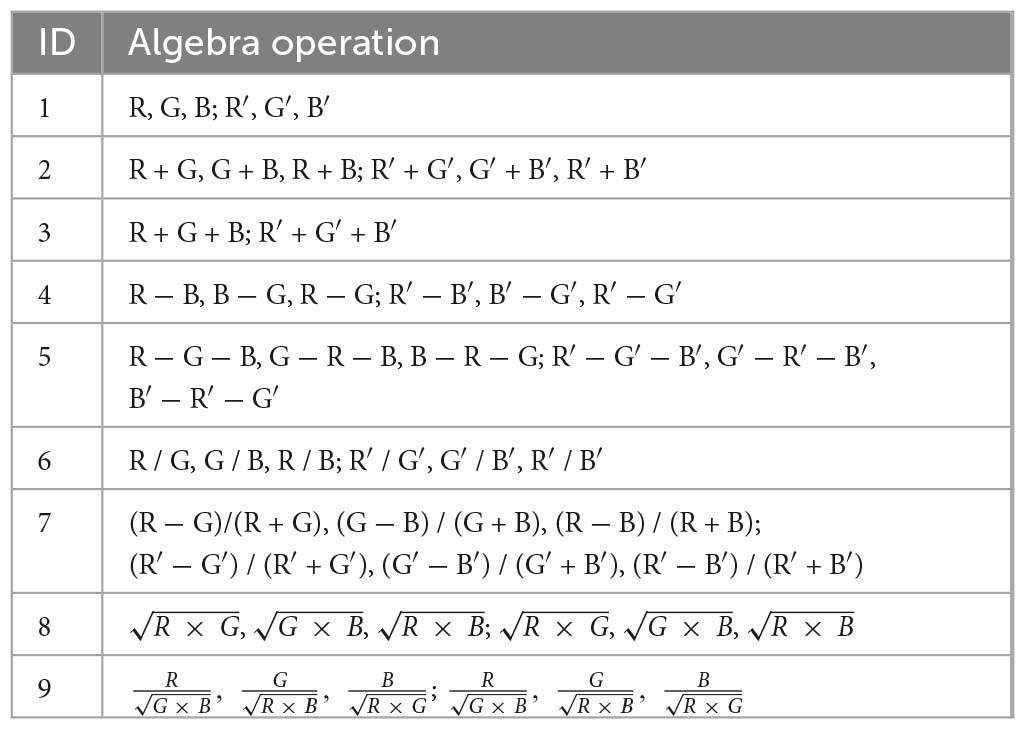
Table 2. Equation combinations of the original and normalized green, red, and blue band information in the BSV images.

where G, R, and B represent the normalized G, R, and B band values of the BSV images; G_pixel, R_pixel, and B_pixel are the corresponding band values; G_min, R_min, and B_min denote the minimum band values, and G_max, R_max, and B_max are the maximum band values.

Subsequent to the NVGI calculation, the grayscale images were obtained and the NVGI value ranges of green vegetation and other features can be identified. The green vegetation area in each image was then distinguished based on the segmentation method (AlSaeed et al., 2016), in which the pixels of each image are represented in L gray levels [1,2,…L], the number of pixels at level i is represented by n_i, and the total number of pixels using N = n₁+n₂+….n_L. The probability distribution is:

$p_i=\frac{n_i}{N},p_i\ge 0,\sum _{i=1}^L{p}_i=1(3)$

If the image is classified into two classes C₀ and C₁ by a threshold at level t, C₀ is the pixels with gray levels [1,2…,t] and C₁ is [t+1,….L]. The probability of class occurrence and class means are:

${\mathrm{\omega }}_0=p_r\left(C_0\right)=\sum _{i=1}^t{p}_i=\mathrm{\omega }(t){\mathrm{\mu }}_0=\sum _{i=1}^{t}i{p}_i(i\backslash C_0)(4)$

$=\sum _{i=1}^{t}i\frac{p_i}{{\mathrm{\omega }}_0}=\frac{\mathrm{\mu }(\mathrm{t})}{\mathrm{\omega }(t)}\hspace{0.17em}$

$\hspace{0.17em}{\mathrm{\omega }}_1=p_r\left(C_1\right)=\sum _{i=t+1}^L{p}_i=-\mathrm{\omega }(t){\mathrm{\mu }}_1=(5)$

$\sum _{i=t+1}^{L}i{p}_r(i\backslash C_1)=\sum _{i=t+1}^{tL}\frac{p_r}{{\mathrm{\omega }}_1}=\frac{{\mathrm{\mu }}_T-\text{ì}(\mathrm{t})}{1-\mathrm{\omega }(t)}\hspace{0.17em}$

where ω₀ and μ₀, ω₁ and μ₁ are the zeroth and first-order cumulative moments of the histogram up to the t-th level and are defined as follows:

$\mathrm{\omega }(t)=\sum _{i=1}^t{p}_i\mathrm{\mu }(t)=\sum _{i=1}^{t}i{p}_i(6)$

μ_T is the total mean level of the original image which is computed as:

$\hspace{0.17em}{\mathrm{\mu }}_T=\text{ì}\left(\text{L}\right)=\sum _{i=1}^{t}i{p}_i(7)$

${\mathrm{\mu }}_0{\mathrm{\omega }}_0+{\mathrm{\mu }}_1{\mathrm{\omega }}_1={\mathrm{\mu }}_T,{\mathrm{\omega }}_0+{\mathrm{\omega }}_1=1(8)$

The class variances and total variance are computed using the equations below:

$\mathrm{\sigma }_0{}^2=\sum _{i=1}^t{(i-{\mathrm{\mu }}_0)}^2{p}_r(i\backslash C_0)=\sum _{i=1}^t{(i-{\mathrm{\mu }}_0)}^2\frac{p_i}{{\mathrm{\omega }}_0}(9)$

$\mathrm{\sigma }_1{}^2=\sum _{i=t+1}^L{(i-{\mathrm{\mu }}_1)}^2{p}_r(i\backslash C_1)=\sum _{i=1}^t{(i-{\mathrm{\mu }}_1)}^2\frac{p_i}{{\mathrm{\omega }}_1}(10)$

To evaluate the threshold (at level t), the within-class variance ($\mathrm{\sigma }_w{}^2$) and between-class variance ($\mathrm{\sigma }_B{}^2$) is used as measures of class, separability, and their equations are as follows.

$\hspace{0.17em}\mathrm{\sigma }_w{}^2={\mathrm{\omega }}_0\mathrm{\sigma }_0{}^2+{\mathrm{\omega }}_1\mathrm{\sigma }_1{}^2(11)$

$\mathrm{\sigma }_B{}^2={\mathrm{\omega }}_0{({\mathrm{\mu }}_0-{\mathrm{\mu }}_T)}^2+{\mathrm{\omega }}_1{({\mathrm{\mu }}_1-{\mathrm{\mu }}_T)}^2={\mathrm{\omega }}_0{\mathrm{\omega }}_1{({\mathrm{\mu }}_1-{\mathrm{\mu }}_0)}^2(12)$

in which

$\hspace{0.17em}\mathrm{\eta }=\frac{\mathrm{\sigma }_B{}^2}{\mathrm{\sigma }_T{}^2}(13)$

$\mathrm{\sigma }_T{}^2=\mathrm{\sigma }_w{}^2+\mathrm{\sigma }_B{}^2(14)$

As $\mathrm{\sigma }_B{}^2$is dependent on first order statistics, while $\mathrm{\sigma }_w{}^2$ depends on the second order statistics. Therefore, $\mathrm{\sigma }_B{}^2$is the simplest measure for t. Thus, η(t) is adopted as the criterion measure to select the best threshold value (t) which is determined by a sequential search using the following functions.

$\hspace{0.17em}\mathrm{\eta }(\mathrm{t})=\frac{\mathrm{\sigma }_B{}^2(t)}{\mathrm{\sigma }_T{}^2}(15)$

$\mathrm{\sigma }_B{}^2\left(t\right)=\frac{{\left[{\mathrm{\mu }}_T\mathrm{\omega }\left(t\right)-\mathrm{\mu }\left(t\right)\right]}^2}{\mathrm{\omega }\left(t\right)\left[1-\mathrm{\omega }\left(t\right)\right]}(16)$

Considering $\mathrm{\sigma }_T{}^2$ is not a function of threshold (t), the optimal threshold should be the value that maximizes the between-class variance [$\mathrm{\sigma }_B{}^2(t)$]. Thus the optimal threshold value (t*) can be computed with the equation below.

$\mathrm{\sigma }_B{}^2\left(t^{*}\right)=max\left[\mathrm{\sigma }_B{}^2(t)\right],t\ge 1\mathrm{and}<\text{L}(17)$

The support vector machine (SVM) classification method was used as a comparison to distinguish the green vegetation pixels based on the spectral information of the BSV images, which is a typical conventional classification approach for multi-spectral images (Ding et al., 2016). To maximize the distance between the hyperplane and the nearest pixel in each of the two groups, it divides pixels into two groups using hyper planes (Vapnik, 1999). Up until a pair of pixels has the closest distance in various classes, the SVM classification operations are repeated. The key issue that makes SVM difficult to automate is that it is a type of supervised classification approach that requires the user to designate classes of interest and train the classifier before the classification (Woodard, 1992; Samiappan and Moorhead, 2015). In this study, the kernelType was RBF, the gamma was set to 0.5, and the cost was 10. Another 200 randomly chosen BSV images were visually interpreted in this study to create a set of reference data for training the SVM classifier (Lillesand et al., 2015).

Two hundred new BSV images were used to create the verification dataset, which served as a means of validating the identification findings obtained using the NVGI-based and SVM methods. These BSV images’ green vegetation was manually portrayed and utilized as a reference. The confusion matrix (user’s, producer’s, and overall accuracy) and the Kappa coefficient were used to evaluate the correctness of the results generated by the NVGI and SVM methods. When compared to the total number of pixels, the user’s accuracy indicates how many pixels accurately reflect a given class; the producer’s accuracy indicates how many portions of a given class were correctly represented in the categorized image (Tung and LeDrew, 1988). The proportion of correctly categorized pixels to all pixels is known as the overall accuracy. Along with the overall consistency between the reference and classified images, the Kappa coefficient also considers incorrectly classified pixels from the error matrix (Rosenfield and Fitzpatrick-Lins, 1986).

$\widehat{k}=\frac{N{\sum }_{i=1}^r{X}_{ii}-{\sum }_{i=1}^r{X}_{i+}{X}_{+i}}{N^2-{\sum }_{i=1}^r{X}_{i+}{X}_{+i}}(18)$

where r represents the number of rows and columns in the confusion matrix, N is the total number of elements, X_ii is the elements in row i and column i, X_i+ is the marginal total of row i, and X_+i is the marginal total of column i.

3.3. Greenery quantification and gradation

The green view index (Deng et al., 2021) was used here to quantitatively describe and compare the green vegetation distribution pattern of each sampling site. The green view index is defined as the proportion of green vegetation pixels in the BSV image, its computation equation is shown below.

$\text{G}\mathrm{reen}\mathrm{view}\mathrm{index}=\frac{N_{veg}}{N_{total}}\times 100(19)$

where N_veg represents the pixel amount of green vegetation in each BSV image, it can be identified using the NVGI method and counted automatically; N_total means the total pixels of each BSV image, which is a constant value in this study (1,521,216 pixels). After the procedure of green view index computation, the sampling sites were further classified into four different levels based on the green view index computation results and the gradation system of extant studies (Aoki, 1987; Yu et al., 2019) with an interval of 10% (Table 3).

TABLE 3

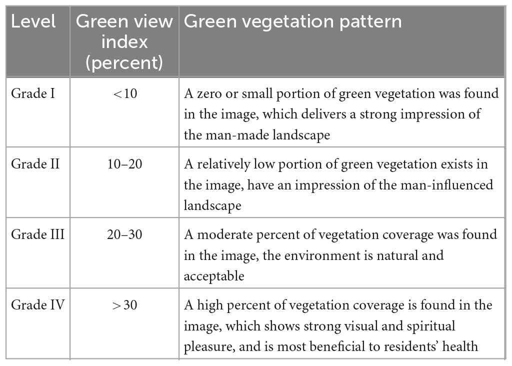
Table 3. Criteria green view index derived system of vegetation greenery in the study site.

3.4. Spatial analysis methods

Moran’s I and Getis-Ord GI* analysis were employed to analyze the spatial distribution patterns of the green view index. The global Moran’s I is a measure of the overall clustering of the spatial data (Moran, 1950). Compared with the global spatial autocorrelation, the local Moran index calculates the spatial correlation degree between each spatial object in the analysis region and its neighboring objects, analyzes the local characteristic differences in the distribution of spatial objects, and reflects the spatial heterogeneity and instability in the local region (Anselin, 1995). They are defined as:

$\text{I}=\frac{N}{W}\frac{{\sum }_{i=1}^N{\sum }_{j=1}^N{w}_{ij}(x_i-\overline{x})(x_j-\overline{x})}{{\sum }_{j=1}^N{(x_i-\overline{x})}^2}\text{I}=\sum _{i=1}^N\frac{I_i}{N}(20)$

where I is the Global Moran’s I measuring global autocorrelation, and I_i is local; N is the number of spatial units indexed by i and j; x is the variable of interest; $\overline{x}$is the mean of x; w_ij is a matrix of spatial weights with zeroes on the diagonal; and W is the sum of all w_ij.

The hot spot analysis tool calculates the Getis-Ord Gi* statistic for each feature in a dataset. It is an effective means to explore the characteristics of local spatial clustering distribution, which can distinguish the degree of clustering of variable spatial distribution by cold and hot spots (Getis and Ord, 2010). The Gi* statistic returned for each feature in the dataset is a z-score. For statistically significant positive z-scores, the larger the z-score is, the more intense the clustering of high values (hot spots); the lower the z-score is less than 0, the more intense the clustering of low values (cold spots).

The Getis-Ord local statistic is given as:

${\text{G}}_i^{*}=\frac{{\sum }_{j=1}^n{w}_{i,j}{x}_j-\overline{X}{\sum }_{j=1}^n{w}_{i,j}}{S\sqrt{\frac{\left[n{\sum }_{j=1}^n{w}_{i,j}^2-{({\sum }_{j=1}^n{w}_{i,j})}^2\right]}{n-1}}}\overline{X}=\frac{{\sum }_{j=1}^n{w}_{i,j}}{n}(21)$

$\text{S}=\sqrt{\frac{{\sum }_{j=1}^n{x}_j^2}{n}-{(\overline{X})}^2}\hspace{0.17em}$

where x_j is the attribute value for feature j, w_i,j is the spatial weight between feature i and j, n is the total number of features.

4. Results

4.1. NVGI calculation

The original value ranges of the 200 BSV images were shown in Figure 2A. Spectral ranges of vegetation greenery and other common features, including shade, poles, vehicles, buildings, and pavement, are largely overlapped, which reduces the value of the images as a source of data for identifying vegetation. After the normalization process, the features can be separated into two groups, as shown in Figure 2B, the pixel values of vegetation greenery and green shade were different from those of other features. The NVGI computation results were obtained using Equation 2 and shown in Figure 2C. The NVGI value range of green vegetation in the study area is 1.06–1.32, which is different from that of the sky, shade, pole, vehicles, building facade, and pavement. Based on the NVGI differences, the green vegetation pixels in the BSV images can be identified.

FIGURE 2

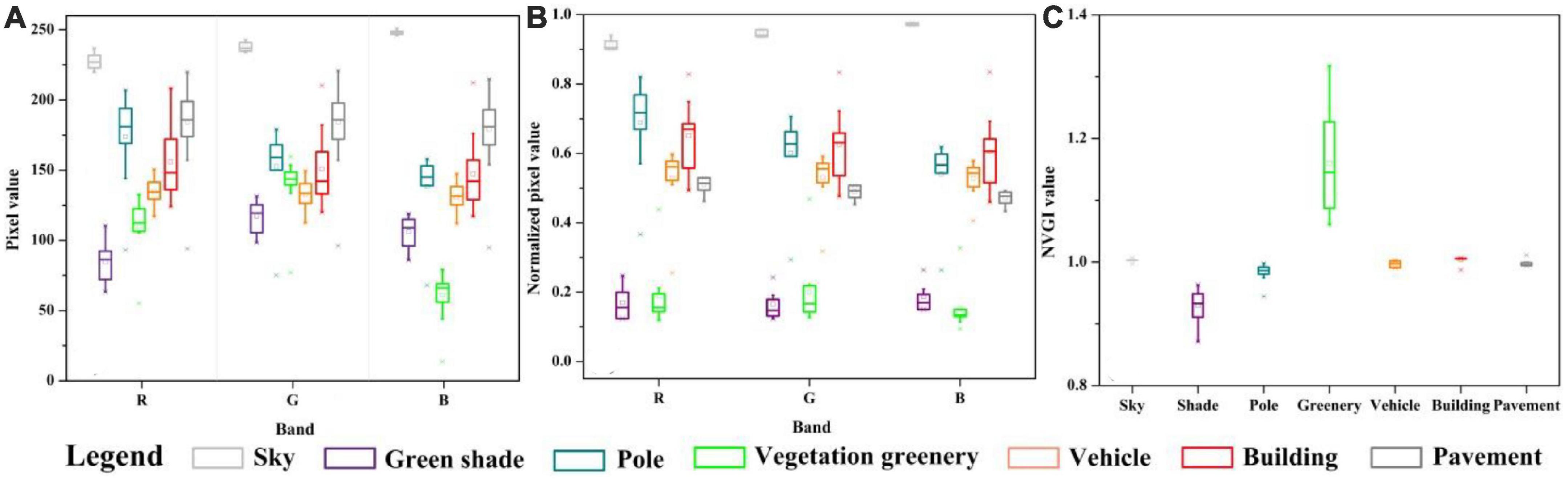
Figure 2. Normalized Vegetation Greenery Index value ranges of common features existing in the BSV image. (A) Original pixel values of the common features in the BSV images, (B) normalized pixel values of the common features, and (C) NVGI values of the common features.

4.2. Verification of vegetation greenery identification

The NVGI method was applied to the 7,695 BSV images, and the findings were saved in the GIS database for subsequent study. In two randomly chosen BSV images, shown in Figure 3, the vegetation greenery was extracted using the NVGI, SVM, and manual identification methods to display the extraction findings. White was used to symbolize the green vegetation, while black was used to represent the other features. Green vegetation in the BSV images may be distinguished in the NVGI-based method with high accuracy when compared to the SVM and the reference (the manual method). When employing the NVGI approach, for example, it is possible to identify artificial green features as non-vegetation, such as the vehicles (Figure 3b). However, the SVM-derived results incorrectly classify the green vegetation with other features (Figures 3c, g).

FIGURE 3

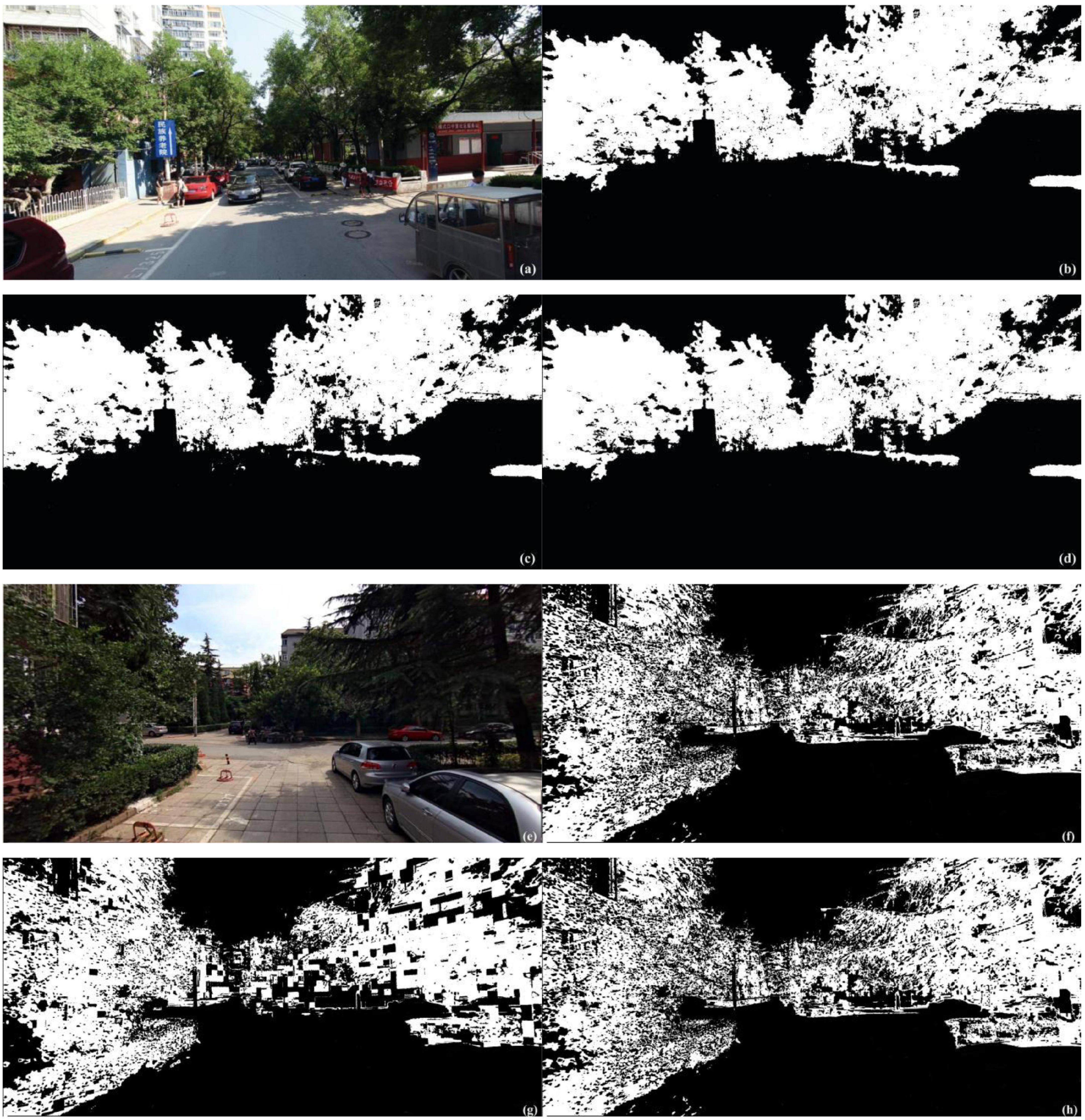
Figure 3. Comparison of green vegetation identification results of the BSV images. (a,e) The original BSV images, (b,f) extraction results using NVGI-based method, (c,g) SVM method, and (d,h) manual results.

To further verify the accuracies of the NVGI-based and the SVM method, another 200 BSV images were randomly selected from the BSV image dataset. All the images were manually classified by using the polygon partitioning function in the ArcGIS Desktop^® 10.1 (Environmental Systems Research Institute, Inc., Redlands, CA, USA). The classification accuracies of these images were computed, and the green vegetation identification results (dependent variable) with the manual depiction ones (independent variable) were compared. As shown in Table 4, the NVGI method improved the accuracy of vegetation greenery identification by 18% (Kappa of 0.85 vs. 0.72) and 20% (Overall Accuracy of 0.91 vs. 0.76), compared to the SVM methods (Table 4), which is more suited for vegetation greenery identification in the street view images. The results using NVGI-based and SVM methods were then compared with the manually depicted maps. In the fitting results (Figure 4), the red dashed lines are the fitting ones between the independent and dependent variables. The regression line of the NVGI-based method and manual results is close to the diagonal line, and Pearson’s r = 0.993, with p = 0.000, shows that the green vegetation classification made using the NVGI method was closely correlated with those of the reference classification (Figure 4A); the SVM extracted green view indexes were overestimated compared to the manual ones (Figure 4B). The vegetation greenery index values computed using the NVGI-based method were consistent with the artificial refinement, which can be used in further spatial analysis.

TABLE 4

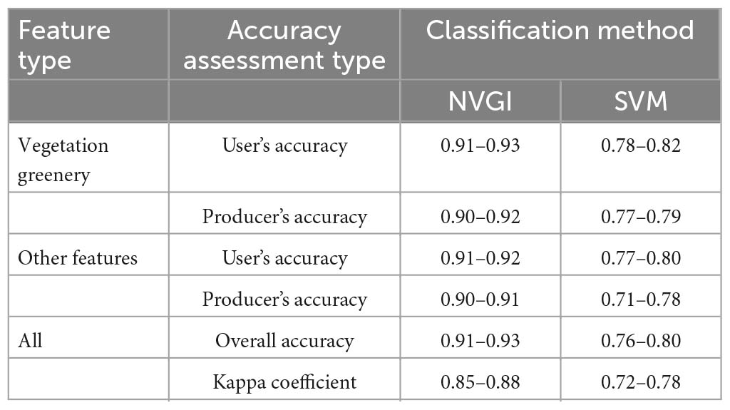
Table 4. Accuracy of vegetation greenery classification using the NVGI and SVM methods.

FIGURE 4

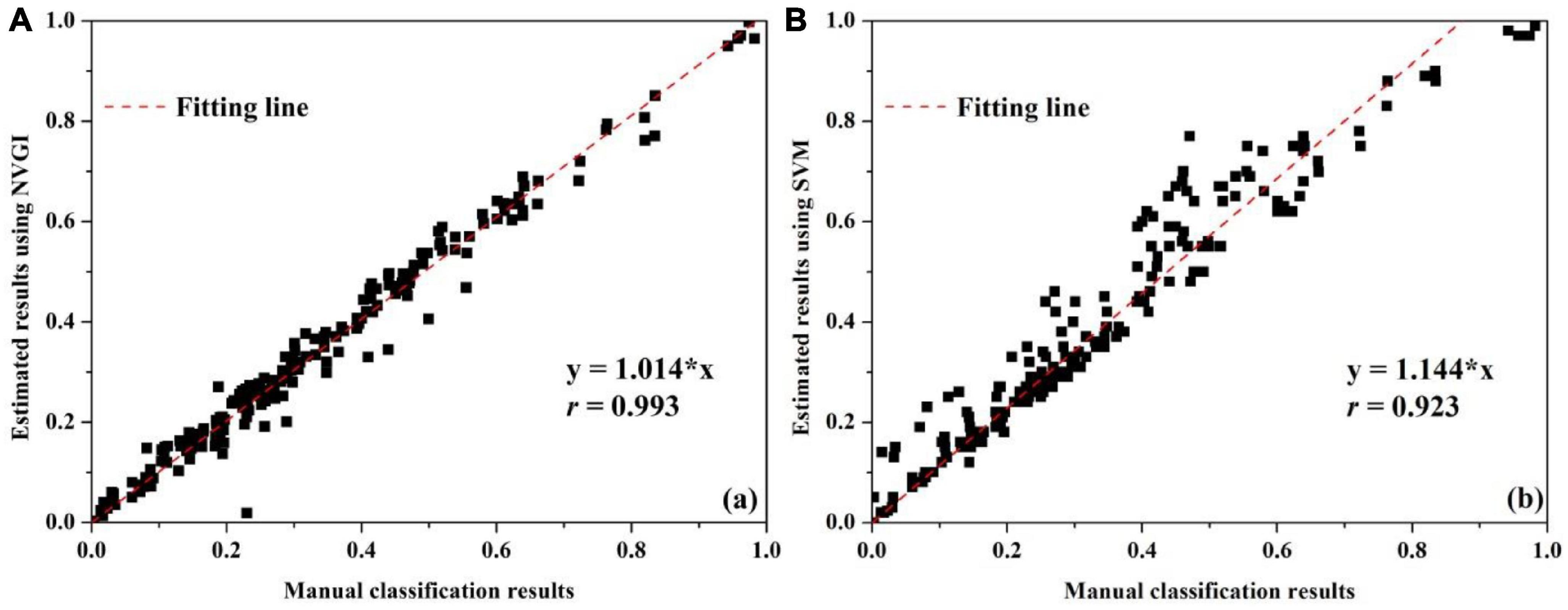
Figure 4. Agreement between the vegetation greenery index values obtained from the vegetation greenery classification made using the NVGI-based and manual methods (A), SVM, and manual methods (B).

4.3. Spatial distribution of vegetation greenery

The green view index of each sampling site was computed and shown in Figure 5. The dot color represented the percentage of green vegetation in each sampling site, in which red and orange colors indicated low and relatively low green vegetation in the study area, respectively, and green and blue color dots represented the moderate and high green vegetation distribution. It can be found that the sample sites were not evenly distributed within green index grades (Table 5). Sampling sites classified as Grade II and III accounted for more than 60% of the total sites, which indicated that the communities in the study area were not green enough for residents’ sensory and psychological health. Among them, 2,440 sampling sites (31.70%) were classified as Grade II, which had relatively low proportions (10–20%) of vegetation greenery in these BSV images, the residents in the communities may have an impression of relatively low greenery and high man-influenced landscape; 2,469 sites (32.09%) were classified as Grade III, i.e., moderate greenery with 20–30% portions in the BSV images, in which the artificial environment is natural due to the relatedly high proportion of greenery (Table 5). In addition, 584 sites (75.90%) were found to have small proportions of green vegetation (0–10%) in the images, in which 211 sampling sites were found with no green vegetation planted (0%), residents standing or walking past these sites will have a strong perspective of the man-made landscape. A total of 28.62% (2,202) sites had a high percentage of vegetation coverage, showing strong visual and spiritual pleasure.

FIGURE 5

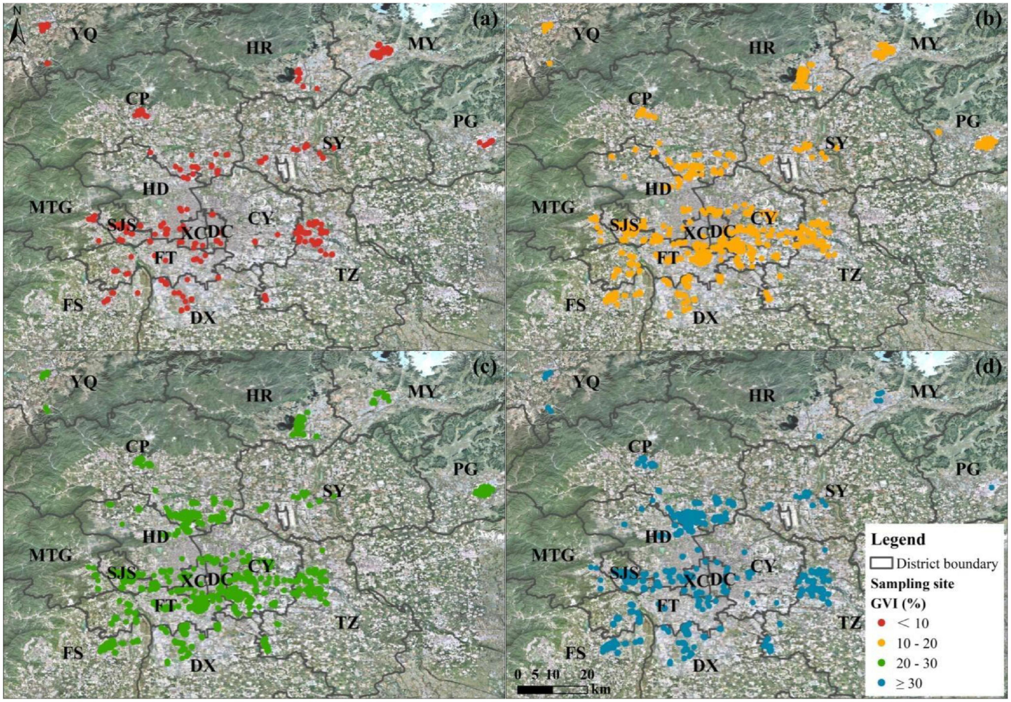
Figure 5. Spatial distribution of green view index Grade I (a), II (b), III (c), and IV (d).

TABLE 5

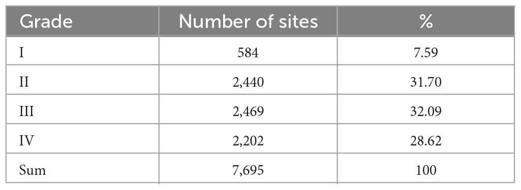
Table 5. Gradation of green view index in the study area.

The vegetation greenery among the sixteen districts varied and showed different spatial distribution patterns, which can be classified into three categories (Table 6): (1) In CP, SJS, FS, HD, DX, and TZ, the prevalent green view index grades were Grade IV (green view index ≥30%), and Grade III (green view index ∈[20%, 30%), Table 6), residents living in these districts may encounter more visible green vegetation when they stand or walk along the inner roads of the communities. (2) In CY, DC, FT, HR, MTG, PG, SY, and XC, the main grades of the green view index were Grade III [green view index ∈(20%, 30%)] and Grade I [green view index ∈(10%, 20%)], the residential communities in these eight districts appeared less green than those in the aforementioned six districts (Figure 5). (3) As for the left two districts (MY and YQ), the dominant grades were Grade I (green view index less than 10%), which meant the residential communities in these two districts lacked green vegetation.

TABLE 6

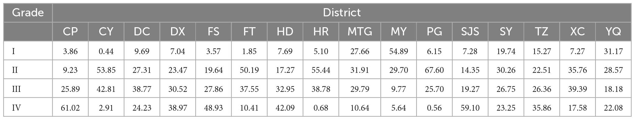
Table 6. The proportion of green view index gradation in each district (%).

4.4. Spatial analysis of vegetation greenery

The Moran’s I value of all green view index values based on the NVGI method in the study area (0.476, p = 0.000) demonstrated that the green view index values have positive spatial autocorrelation. Local Moran’s I analysis showed that High-High and Low-Low cluster types prevailed in the study area (Figure 6 and Table 7). Among the 467 sample sites in SJS, 260 exhibited a high-high cluster, accounting for 55.7%, which is the highest percentage in the high-high cluster type. A high-high cluster was present in 557 sample sites in CP, accounting for 52.4%; which was also present in FS and DX, accounting for 32.8 and 32.1%, respectively. In terms of the low-low cluster type, 213 of 266 sample sites in Miyun showed a low-low cluster, accounting for 80.1%. HR and CY followed, with 68 and 59.6%. Five hundred eighty-five of 1028 sample sites in FT showed a low-low cluster, accounting for 56.9%. In addition, the percentage of PG low-low clustering sites was 56.4% (Table 7).

FIGURE 6

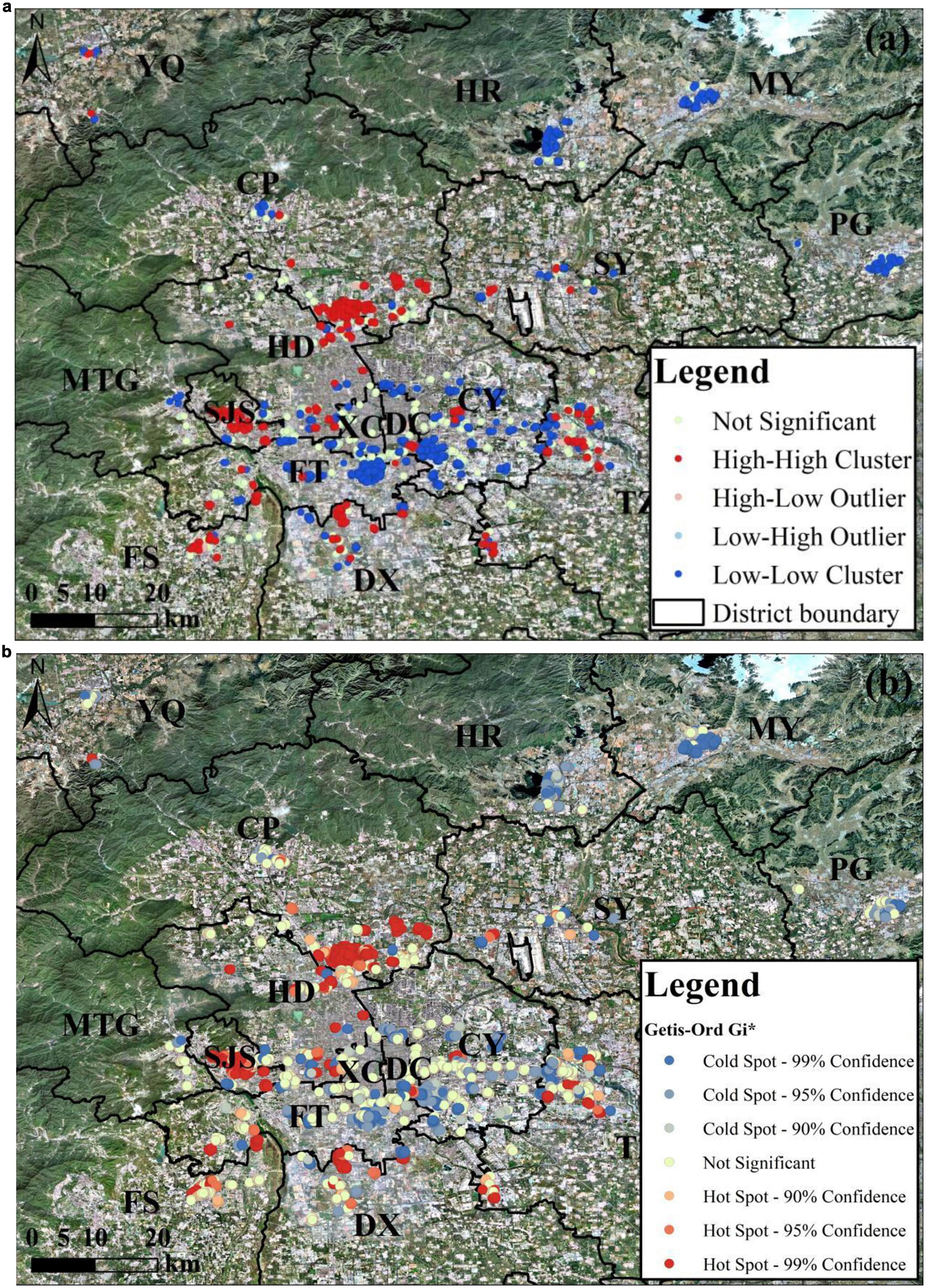
Figure 6. Local Moran’s I (a) and Getis-Ord GI* (b) of green view index in the study area.

TABLE 7

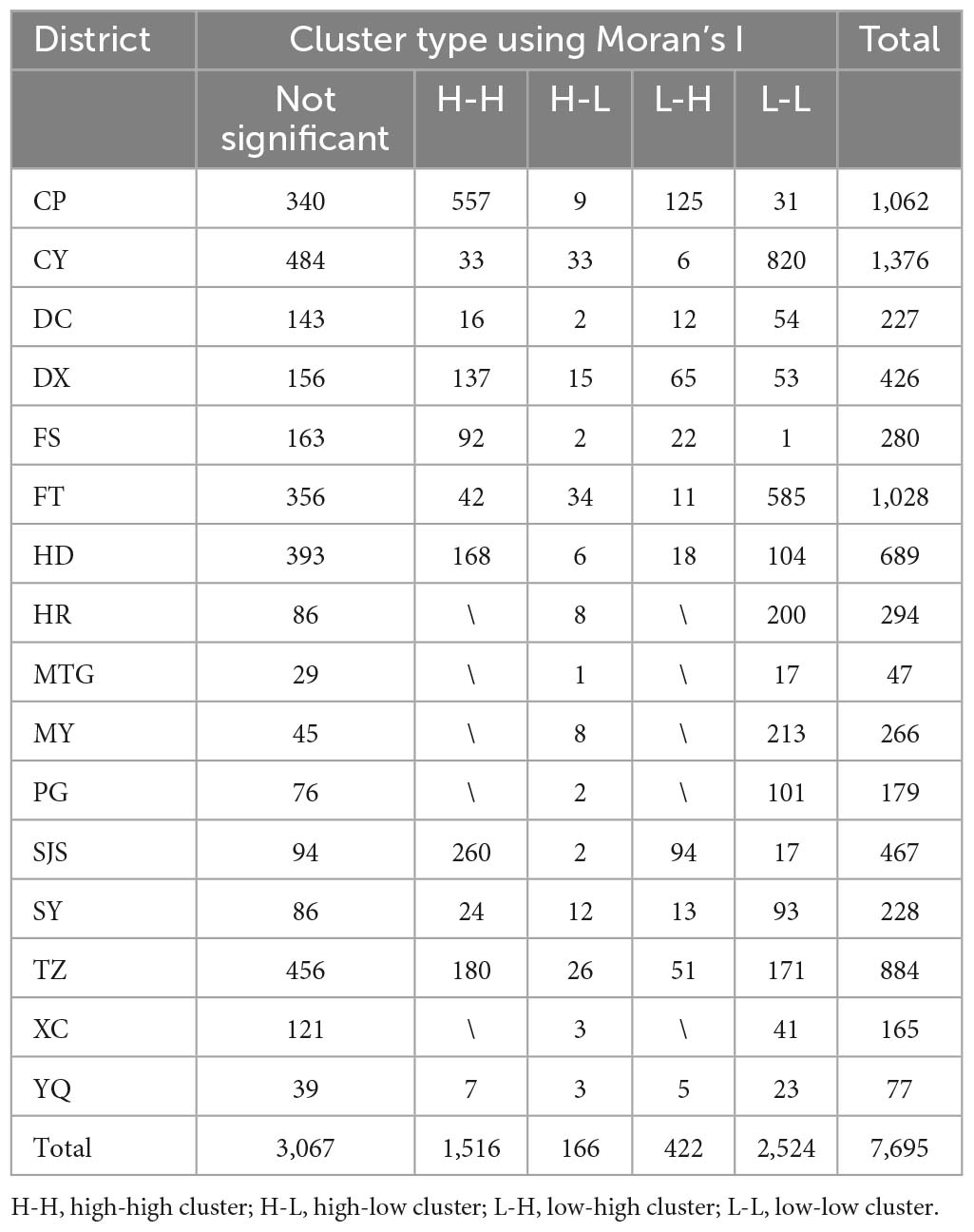
Table 7. Cluster types using local Moran’s I in the study area.

The Getis-Ord GI* analysis was used to detect cold and hot spots of green view index values in the study area. Figure 6b showed whether the spatial clustering of the sampling sites was significant and, if so, at what level (0.01, 0.05, and 0.1 levels). The spatial weight matrix was calculated based on the Euclidean distance between sampling sites, the distance threshold was 485.447 m. The spatial heterogeneity analysis found that the core region of the study area (DC and XC), the core area of the suburban district, such as HR, MY, PG, and MTG, presented low-value clustering (cold spots, 3,205 sampling sites). Conversely, the peripheral zone (e.g., CP and SJS) surrounding the core area mainly presents high-value clustering (hot spots, 2,304 sites).

5. Discussion

This is the first study that concentrated in monitoring greenery characteristics in residential communities. The identification and spatial analysis of vegetation greenery were conducted using an NVGI-based method and street view images. The study area consisted of all residential communities that have the street view images. The results demonstrated that the proposed method can extract additional spectral information from the street view RGB images (i.e., BSV images) to improve the classification and evaluation accuracy of vegetation greenery without NIR information. The green vegetation exhibited distinct spatial heterogeneity in the study area. The main contributions of this study are (1) to propose a new path to monitor the spatial variations of vegetation greenery in residential communities and (2) to improve the accuracy of greenery classification and evaluation, which is overlooked by existing studies.

5.1. Image acquisition

Baidu street view imagery uses people’s profile optic angle and view, which is different from those of conventional satellite RS images, to capture and record images. Consequently, BSV images are unable to capture green spaces such as green roofs that cannot be observed or detected from a road angle (Yu et al., 2022). However, BSV images enable it to be used to measure vegetation greenery from the viewpoint of people who are standing or walking on the roads, it can be more useful in residential community planning and management. During the image acquisition process, BSV images captured in alignment with the direction of a road’s heading were selected for analyzing vegetation’s greenery. This approach to image selection can enhance the effectiveness and accuracy of vegetation greenery analysis when dealing with varying road widths (Han et al., 2013; Chen et al., 2020). Previous studies employed multiple images (e.g., 18 images: 6 horizontal directions and 3 aspects in each direction; or 12 images: 4 horizontal directions and 3 aspects in each direction) to mitigate the impact of road width on vegetation greenery at a specific location of interest (Li et al., 2015; Chen et al., 2019; Yu et al., 2019). The extensive requirements for image or data can result in time-consuming and labor-intensive analysis of vegetation greenery. In contrast, the proposed method only requires BSV images facing the direction of the road while minimizing potential errors due to variations in road width.

5.2. Comparison with existing methods

Using the grid-overlay method, the initial urban street green vegetation studies manually identified and measured vegetation greenery from profile images (e.g., Shafer et al., 1969; Nordh et al., 2009). Multi-spectral classification techniques were also developed in conjunction with the creation of RS images to increase the effectiveness and precision of identifying green vegetation from datasets of profile images (Li et al., 2017; Lu, 2019). However, the direct application of the conventional supervised approaches (such as SVM in this study) results in misclassification of vegetation greenery with other common features in the BSV images due to the absence of the NIR band and the spectral overlap of R, G, and B bands. In contrast, the NVGI methodology efficiently extracts more valuable spectral information from the BSV images in comparison to the traditional SVM method, improving the recognition accuracy of green vegetation.

Unlike previous studies that monitored urban street-side greenery using satellite RS images, such as Landsat and Sentinel series data, to compare the extracted green view index results with the typical NDVI (Normalized Difference Vegetation Index), this study did not utilize such methods due to the narrower roads within the residential communities under study, which have a width of less than 4 m. This is in contrast to trunk roads which can be as wide as 30 m, secondary trunk roads at 12 m and side roads at 8 m. Unfortunately, commonly used Landsat-8/9 and Sentinel-2A/B satellite imagery that is available for free download have a pixel size ranging from 10 to 60 m, rendering them unsuitable for conducting comparisons due to their low resolution.

5.3. Cause of low green view indexes

Population growth in cities combined with urban planning policies of densification may drive the conversion of vegetation-planted areas into residential land (Kabisch and Haase, 2014; Weber et al., 2017). The findings of this study indicated that more than 60% of the study sites had low green view indexes. According to the data from the Bureau of Statistics, these residential communities were constructed between 1995 and 2010. Due to their construction period and design philosophy, the issue of massive car ownership was not fully taken into consideration (Frank et al., 2010; Xiao et al., 2021). In many regions of the study area, property management skills and levels were also insufficient. Consequently, private buildings have replaced the community’s open green space (Li and Zhao, 2017; Mandeli, 2019). These factors contribute to the comparatively low levels of greenery in the study area. To achieve better community management and promote residential greenery equality, it is essential to conduct timely and accurate community greenery monitoring.

5.4. Application of the proposed framework

The NVGI method was proposed to conduct vegetation extraction, whereby the R, G, and B band values were initially normalized to minimize the pixel value discrepancies of identical features in the BSV images. Subsequently, the NVGI was employed to amplify differences between distinct features and identify greenery within the BSV images, as depicted in Figure 2. It allows planners to identify the name and location of residential communities that contain few green areas (especially the zero-value areas). By analyzing the results, these areas can be identified and improved through various measures such as clearing privately occupied areas and implementing structural systems that facilitate the growth of plants like trees, shrubs, and lawns on vertical surfaces (Ghazalli et al., 2019; Chan et al., 2021). Currently, the BSV images have covered 424 cities in China. The proposed framework in this study can be directly applicable to multi-year BSV images, facilitating landscape planners’ evaluation of urban vegetation greenery and its variations. Furthermore, the proposed framework can be utilized in other cities and countries that have street view images (e.g., Google street view image, Tencent street view image, etc.) to explore the greenery characteristics of residential areas.

5.5. Limitations

Although the proposed method enables monitoring of spatial variations in vegetation greenery within residential communities and improve the accuracy of greenery classification and evaluation, this study is not without limitations. Firstly, due to the prolonged impact of the COVID-19 pandemic in China, data on in situ community characteristics such as the facade of the building structure and resident opinions regarding green view index grading were temporarily unavailable for collection. This issue will be addressed in a future study through the implementation of additional interviews and research. Furthermore, the utilization of random sampling to establish study sites may have an impact on the accuracy of Getis-Ord Gi* spatial analysis due to variations in resident age grades and building construction dates among communities. More comprehensive investigations should be conducted to compare the outcomes obtained from different spatial sampling modes. Additionally, in this study, trees and grasses were not distinguished separately in BSV images due to their similar impacts on human pleasure and shared spectral change patterns within the study area. Future research will focus on examining their variations during other seasons and discussing their identification and correlation with NVGI individually.

6. Conclusion

This study examined the usability of an NVGI-based method in the identification and monitoring of vegetation greenery in residential communities. The results found that the combination of BSV image and NVGI-based method can extract green vegetation efficiently. Vegetation greenery exhibited spatial heterogeneity in the study area. The finding of this study can help understand vegetation greenery supportiveness and be used as a reference for greenery management and planning in residential communities. Further study will be done on the seasonal and annual variation of vegetation greenery in more residential communities to provide temporal reference information for residential community planning.

Data availability statement

The original contributions presented in this study are included in the article/supplementary material, further inquiries can be directed to the corresponding authors.

Author contributions

XY and XZ: conceptualization and writing—review and editing. JS: methodology and validation. XY: manual classification. JS and XY: writing—original draft. All authors read and agreed to the published version of the manuscript.

Funding

This study was supported by the greenery rating based on the visual perspective of residents (2020skx053). The supporters had no role in the study design, data collection, analysis, decision to publish, or preparation of the manuscript.

Acknowledgments

We thank the reviewers for their constructive comments on the manuscript.

Conflict of interest

The authors declare that the research was conducted in the absence of any commercial or financial relationships that could be construed as a potential conflict of interest.

Publisher’s note

All claims expressed in this article are solely those of the authors and do not necessarily represent those of their affiliated organizations, or those of the publisher, the editors and the reviewers. Any product that may be evaluated in this article, or claim that may be made by its manufacturer, is not guaranteed or endorsed by the publisher.

Footnotes

1. ^ http://lbsyun.baidu.com

References

AlSaeed, D. H., Bouridane, A., and El-Zaart, A. (2016). A novel fast otsu digital image segmentation method. Int. Arab J. Inf. Technol. 13, 427–434.

Google Scholar

Anselin, L. (1995). Local indicators of spatial association—LISA. Geogr. Anal. 27, 93–115. doi: 10.1111/j.1538-4632.1995.tb00338.x

CrossRef Full Text | Google Scholar

Aoki, Y. (1987). Relationship between visual field and greenness. Garden. Magaz. 51, 1–10. doi: 10.5632/jila1934.51.1

PubMed Abstract | CrossRef Full Text | Google Scholar

Baidu (2020). Baidu map panorama, the world is at your fingertips. Available online at: https://quanjing.baidu.com/#/

Google Scholar

Cai, Y., Chen, Y., and Tong, C. (2019). Spatiotemporal evolution of urban green space and its impact on the urban thermal environment based on remote sensing data: A case study of Fuzhou City, China. Urban For. Urban Green. 41, 333–343. doi: 10.1016/j.ufug.2019.04.012

CrossRef Full Text | Google Scholar

Chan, S. H. M., Lin, Q., Esposito, G., and Mai, K. P. (2021). Vertical greenery buffers against stress: evidence from psychophysiological responses in virtual reality. Landsc. Urban Plann. 213:104127. doi: 10.1016/j.landurbplan.2021.104127

CrossRef Full Text | Google Scholar

Chen, L., Lu, Y., Sheng, Q., Ye, Y., Wang, R., and Liu, Y. (2020). Estimating pedestrian volume using Street View images: A large-scale validation test. Comput. Environ. Urban Syst. 81:101481. doi: 10.1016/j.compenvurbsys.2020.101481

CrossRef Full Text | Google Scholar

Chen, X., Meng, Q., Hu, D., Zhang, L., and Yang, J. (2019). Evaluating greenery around streets using baidu panoramic street view images and the panoramic green view index. Forests 10:1109. doi: 10.3390/f10121109

CrossRef Full Text | Google Scholar

Deng, M., Yang, W., Chen, C., Wu, Z., Liu, Y., and Xiang, C. (2021). Street-level solar radiation mapping and patterns profiling using Baidu Street View images. Sustain. Cities and Soc. 75:103289. doi: 10.1016/j.scs.2021.103289

CrossRef Full Text | Google Scholar

Ding, S., Zhang, X., and Yu, J. (2016). Twin support vector machines based on fruit fly optimization algorithm. Int. J. Mach. Learn. Cybern. 7, 193–203. doi: 10.1007/s13042-015-0424-8

CrossRef Full Text | Google Scholar

Engemann, K., Pedersen, C. B., Arge, L., and Svenning, J. (2019). Residential green space in childhood is associated with lower risk of psychiatric disorders from adolescence into adulthood. Proc. Natl. Acad. Sci. U. S. A. 11, 5188–5193. doi: 10.1073/pnas.1807504116

PubMed Abstract | CrossRef Full Text | Google Scholar

Frank, L., Kerr, J., Rosenberg, D., and King, A. (2010). Healthy aging and where you live: community design relationships with physical activity and body weight in older Americans. J. Phys. Act. Health 7, S82–S90. doi: 10.1123/jpah.7.s1.s82

PubMed Abstract | CrossRef Full Text | Google Scholar

Getis, A., and Ord, J. K. (2010). “The analysis of spatial association by use of distance statistics,” in Perspectives on spatial data analysis, eds L. Anselin and S. Rey (Berlin: Springer), 127–145. doi: 10.1007/978-3-642-01976-0_10

CrossRef Full Text | Google Scholar

Ghazalli, A. J., Brack, C., Bai, X., Said, I., and Hanley, R. E. (2019). Physical and non-physical benefits of vertical greenery systems: a review. J. Urban Technol. 26, 1–26. doi: 10.1080/10630732.2019.1637694

CrossRef Full Text | Google Scholar

Griew, P., Hillsdon, M., Foster, C., Coombes, E., Jones, A., and Wilkinson, P. (2013). Developing and testing a street audit tool using Google Street View to measure environmental supportiveness for physical activity. Int. J. Behav. Nutr. Phys. Act. 10, 1–7. doi: 10.1186/1479-5868-10-103

PubMed Abstract | CrossRef Full Text | Google Scholar

Gu, W., Chen, Y., and Dai, M. (2019). Measuring community greening merging multi-source geo-data. Sustainability 11:1104. doi: 10.3390/su11041104

CrossRef Full Text | Google Scholar

Han, B. H., Kwak, J. I., and Kim, H. S. (2013). Influence factors of street environment for provision and management of street green. Kor. J. Environ. Ecol. 27, 253–265.

Google Scholar

Kabisch, N., and Haase, D. (2014). Green justice or just green? Provision of urban green spaces in Berlin, Germany. Landsc. Urban Plann. 122, 129–139. doi: 10.1016/j.landurbplan.2013.11.016

CrossRef Full Text | Google Scholar

Kumar, J., Biswas, B., and Walker, S. (2020). Multi-temporal lulc classification using hybrid approach and monitoring built-up growth with shannon’s entropy for a semi-arid region of rajasthan, India. J. Geol. Soc. India 95, 626–635. doi: 10.1007/s12594-020-1489-x

CrossRef Full Text | Google Scholar

Li, B., Wang, W., Bai, L., Chen, N., and Wang, W. (2019). Estimation of aboveground vegetation biomass based on landsat-8 oli satellite images in the guanzhong basin, China. Int. J. Remote Sens. 40, 3927–3947. doi: 10.1080/01431161.2018.1553323

CrossRef Full Text | Google Scholar

Li, M., Han, S., and Shi, J. (2017). An enhanced ISODATA algorithm for recognizing multiple electric appliances from the aggregated power consumption dataset. Energy Build. 140, 305–316. doi: 10.1016/j.enbuild.2017.02.006

CrossRef Full Text | Google Scholar

Li, S., and Zhao, P. (2017). Exploring car ownership and car use in neighborhoods near metro stations in Beijing: Does the neighborhood built environment matter? Transp. Res. D Transp. Environ. 56, 1–17. doi: 10.1016/j.trd.2017.07.016

CrossRef Full Text | Google Scholar

Li, T., Zheng, X., Wu, J., Zhang, Y., Fu, X., and Deng, H. (2021). Spatial relationship between green view index and normalized differential vegetation index within the Sixth Ring Road of Beijing. Urban For. Urban Green. 62:127153. doi: 10.1016/j.ufug.2021.127153

CrossRef Full Text | Google Scholar

Li, X., Zhang, C., Li, W., Ricard, R., Meng, Q., and Zhang, W. (2015). Assessing street-level urban greenery using Google Street View and a modified green view index. Urban For. Urban Green. 14, 675–685. doi: 10.1016/j.ufug.2015.06.006

CrossRef Full Text | Google Scholar

Lillesand, T., Kiefer, R. W., and Chipman, J. (2015). Remote sensing and image interpretation. Hoboken, NJ: John Wiley & Sons.

Google Scholar

Liu, Y., Wang, R., Lu, Y., Li, Z., Chen, H., Cao, M., et al. (2020). Natural outdoor environment, neighbourhood social cohesion and mental health: Using multilevel structural equation modelling, streetscape and remote-sensing metrics. Urban For. Urban Green. 48:126576. doi: 10.1016/j.ufug.2019.126576

CrossRef Full Text | Google Scholar

Lu, Y. (2019). Using Google Street View to investigate the association between street greenery and physical activity. Landsc. Urban Plann. 191:103435. doi: 10.1016/j.landurbplan.2018.08.029

CrossRef Full Text | Google Scholar

Ma, L., Huang, Y., and Liu, T. (2022). Unequal impact of the COVID-19 pandemic on mental health: Role of the neighborhood environment. Sustain. Cities Soc. 87:104162. doi: 10.1016/j.scs.2022.104162

PubMed Abstract | CrossRef Full Text | Google Scholar

Mandeli, K. (2019). Public space and the challenge of urban transformation in cities of emerging economies: Jeddah case study. Cities 95:102409. doi: 10.1016/j.cities.2019.102409

CrossRef Full Text | Google Scholar

Moran, P. A. (1950). Notes on continuous stochastic phenomena. Biometrika 37, 17–23. doi: 10.1093/biomet/37.1-2.17

CrossRef Full Text | Google Scholar

Nordh, H., Hartig, T., Hagerhall, C. M., and Fry, G. (2009). Components of small urban parks that predict the possibility for restoration. Urban For. Urban Green. 8, 225–235. doi: 10.1016/j.ufug.2009.06.003

CrossRef Full Text | Google Scholar

Rosenfield, G. H., and Fitzpatrick-Lins, K. (1986). A coefficient of agreement as a measure of thematic classification accuracy. Photogrammetr. Eng. Remote Sens. 52, 223–227.

Google Scholar

Samiappan, S., and Moorhead, R. J. (2015). “Semi-supervised co-training and active learning framework for hyperspectral image classification,” in Proceedings of the 2015 IEEE international geoscience and remote sensing symposium (IGARSS), Piscataway, NJ. doi: 10.1109/IGARSS.2015.7325785

CrossRef Full Text | Google Scholar

Shafer, E. L. Jr., Hamilton, J. F. Jr., and Schmidt, E. A. (1969). Natural landscape preferences: a predictive model. J. Leisure Res. 1, 1–19. doi: 10.1080/00222216.1969.11969706

CrossRef Full Text | Google Scholar

Toaha, M., Islam, S., Rahman, C. R., Asad, S. B., Ahmed, T., Proma, M. A., et al. (2020). Automatic Signboard Detection from Natural Scene Image in Context of Bangladesh Google Street View. arXiv [Preprint].

Google Scholar

Tung, F., and LeDrew, E. (1988). The determination of optimal threshold levels for change detection using various accuracy indexes. Photogrammetr. Eng. Remote Sens. 54, 1449–1454.

Google Scholar

Vapnik, V. (1999). The nature of statistical learning theory. Berlin: Springer science & business media. doi: 10.1007/978-1-4757-3264-1

CrossRef Full Text | Google Scholar

Weber, S., Boley, B. B., Palardy, N., and Gaither, C. J. (2017). The impact of urban greenways on residential concerns: Findings from the Atlanta BeltLine Trail. Landsc. Urban Plann. 167, 147–156. doi: 10.1016/j.landurbplan.2017.06.009

CrossRef Full Text | Google Scholar

Wei, Y., Zhang, K., and Ji, S. (2020). Simultaneous road surface and centerline extraction from large-scale remote sensing images using CNN-based segmentation and tracing. IEEE Trans. Geosci. Remote Sens. 99, 1–13. doi: 10.1109/TGRS.2020.2991733

CrossRef Full Text | Google Scholar

Wolch, J. R., Byrne, J., and Newell, J. P. (2014). Urban green space, public health, and environmental justice: The challenge of making cities ‘just green enough’. Landsc. Urban Plann. 125, 234–244. doi: 10.1016/j.landurbplan.2014.01.017

CrossRef Full Text | Google Scholar

Woodard, J. P. (1992). Modeling and classification of natural sounds by product code hidden markov models. IEEE Trans. Sign. Process. 40, 1833–1835. doi: 10.1109/78.143457

PubMed Abstract | CrossRef Full Text | Google Scholar

Woodhouse, I. H. (2017). Introduction to microwave remote sensing. Boca Raton, FL: CRC press. doi: 10.1201/9781315272573

CrossRef Full Text | Google Scholar

Wu, J., Xu, H., Zhang, S., Li, X., Chen, J., Zheng, J., et al. (2021). Joint segmentation and detection of COVID-19 via a sequential region generation network. Pattern Recogn. 118:108006. doi: 10.1016/j.patcog.2021.108006

PubMed Abstract | CrossRef Full Text | Google Scholar

Xiao, L., Wang, W., Ren, Z., Fu, Y., and He, X. (2021). Two-city street-view greenery variations and association with forest attributes and landscape metrics in ne china. Landsc. Ecol. 36, 1261–1280. doi: 10.1007/s10980-021-01210-0

CrossRef Full Text | Google Scholar

Xiao, Y., Zhang, Y., Sun, Y., Tao, P., and Kuang, X. (2020). Does green space really matter for residents’ obesity? A new perspective from Baidu Street View. Front. Public Health 8:332. doi: 10.3389/fpubh.2020.00332

PubMed Abstract | CrossRef Full Text | Google Scholar

Yang, J., Zhao, L., Mcbride, J., and Peng, G. (2009). Can you see green? assessing the visibility of urban forests in cities. Landsc. Urban Plann. 91, 97–104. doi: 10.1016/j.landurbplan.2008.12.004

CrossRef Full Text | Google Scholar

Ye, Y., Richards, D., Lu, Y., Song, X., Zhuang, Y., Zeng, W., et al. (2019). Measuring daily accessed street greenery: A human-scale approach for informing better urban planning practices. Landsc. Urban Plann. 191:103434. doi: 10.1016/j.landurbplan.2018.08.028

CrossRef Full Text | Google Scholar

Yu, X., Her, Y., Huo, W., Chen, G., and Qi, W. (2022). Spatio-temporal monitoring of urban street-side vegetation greenery using Baidu Street View images. Urban For. Urban Green. 2022:127617. doi: 10.1016/j.ufug.2022.127617

CrossRef Full Text | Google Scholar

Yu, X., and Qi, W. (2021). Measuring vegetation greenery in park using iPhone panoramic image and a new green vegetation extraction index. Urban For. Urban Green. 65:127310. doi: 10.1016/j.ufug.2021.127310

CrossRef Full Text | Google Scholar

Yu, X., Zhao, G., Chang, C., Yuan, X., and Heng, F. (2019). BGVI: A new index to estimate street-side greenery using baidu street view image. Forests 10:3. doi: 10.3390/f10010003

CrossRef Full Text | Google Scholar

Zhong, T., Ye, C., Wang, Z., Tang, G., and Ye, Y. (2021). City-scale mapping of urban facade color using street-view imagery. Remote Sens. 13:1591. doi: 10.3390/rs13081591

CrossRef Full Text | Google Scholar