Forests at the fringe: Comparing observed change to projected climate change impacts for five tree species in the Pacific Northwest, United States

Kralicek, Karin; Barrett, Tara M.; Ver Hoef, Jay M.; Temesgen, Hailemariam

doi:10.3389/ffgc.2022.966953

ORIGINAL RESEARCH article

Front. For. Glob. Change, 15 September 2022

Sec. Forest Management

Volume 5 - 2022 | https://doi.org/10.3389/ffgc.2022.966953

This article is part of the Research Topic Monitoring and responding to global change to promote resilient and productive forests through innovative forest inventory View all 9 articles

Forests at the fringe: Comparing observed change to projected climate change impacts for five tree species in the Pacific Northwest, United States

$\r\nKarin Kralicek,*$ Karin Kralicek^1,2*

Tara M. Barrett³

Jay M. Ver Hoef⁴

Hailemariam Temesgen²

¹Forest Inventory and Analysis Program, Rocky Mountain Research Station, Forest Service, United States Department of Agriculture (USDA), Fort Collins, CO, United States
²Forest Measurements and Biometrics Laboratory, Department of Forest Engineering, Resources, and Management, Oregon State University, Corvallis, OR, United States
³Pacific Northwest Research Station, Forest Service, United States Department of Agriculture (USDA), Wenatchee, WA, United States
⁴Marine Mammal Laboratory, Alaska Fisheries Science Center, National Marine Fisheries Service, National Oceanic and Atmospheric Administration (NOAA), Seattle, WA, United States

Rapid climate change over the coming century will impact suitable habitat for many tree species. In response to these changes in climate, areas that become unsuitable will see higher mortality and lower growth and recruitment. Therefore, early detection of demographic trends is critical for effective forest management. Recent 10-year remeasurement data from the United States (US) Department of Agriculture (USDA) Forest Service’s Forest Inventory and Analysis (FIA) Program’s national annual inventory of forest land provides an ideal data set for analyzing such trends over large areas. However, failure to distinguish between areas of future habitat contraction and expansion or persistence when estimating demographic trends may mask species’ shifts. We used remeasurement data to compare observed tree demographic rates with projected impacts of climate change for five important tree species in the Pacific Northwest. Projected impacts were based on spatial-Bayesian hierarchical models of species distributions, which were used to project areas where habitat would persist (remain climatically suitable), expand (become suitable), or contract (become unsuitable) under four future climate scenarios for the 2080s. We compared estimates of mortality and net-growth between these areas of shifting suitability and a naïve division of habitat based on elevation and latitude. Within these regions, we assessed the sustainability of mortality and determined that observational data suggest that climate change impacts were already being felt in some areas by some species. While there is an extensive literature on bioclimatic species distribution models, this work demonstrates they can be adapted to the practical problem of detecting early climate-related trends using national forest inventory data. Of the species examined, California black oak (Quercus kelloggii) had the most notable instances of observed data suggesting population declines in the core of its current range.

Introduction

The geographic distributions of many tree species will shift in response to the rapid climate change occurring within this century (McKenney et al., 2007; Soja et al., 2007; Lenoir et al., 2008; Mathys et al., 2017). As species track more favorable climate conditions, shifts in a species’ range will manifest through areas of migration, persistence, or extirpation. In the nearer-term, areas that become climatically unsuitable for the species may experience decreased growth and increased mortality rates, while areas that become suitable may see increases in growth and regeneration (Rehfeldt et al., 2014a). Such impacts of climate change on species’ ranges have already been observed in some parts of the globe (Mclaughlin et al., 2014; Monleon and Lintz, 2015; Schaphoff et al., 2015; Stanke et al., 2021). For North American tree species, many researchers generally expect impacts of a warming climate to involve range contraction at the low-elevation, southern-limits of a species’ distribution and range expansion at the high-elevation, northern-limits (Bell et al., 2014; Rehfeldt et al., 2014a; Monleon and Lintz, 2015).

Therefore, early detection of demographic trends is critical for effective forest management. The recent availability of 10-year remeasurement field-data from the United States (US) Department of Agriculture (USDA) Forest Service’s Forest Inventory and Analysis (FIA) Program’s national annual inventory of forest land provides a unique opportunity to analyze such trends over large areas. However, shifts in a species’ range may be masked when demographic trends are estimated without distinguishing between areas where habitat is projected to shift in climatic suitability, such as combining areas where habitat is expanding and becoming suitable with areas where it is contracting and becoming unsuitable. In this study, we compare estimates of observed mortality and net-growth to projected shifts in suitable habitat for five tree species in the Pacific Northwest under four future climate scenarios for the 2080s.

Whether or not a species will decline in an area over time is determined by the interplay of tree demographic rates through the balance of mortality with recruitment and growth (Lintz et al., 2016; McDowell et al., 2020; Stanke et al., 2021). While mortality has been used as a forest-change indicator (e.g., van Mantgem et al., 2009), stand development (i.e., the successional development of forest stands) should be considered alongside such demographic rates (Luo and Chen, 2013). At the stand-level, density-dependent mortality or “self-thinning” occurs in early- and mid-successional forests as they age (Franklin et al., 2002). This can result in mortality exceeding growth when measured by the number of trees per ha (TPH). Through this stand-development process, resources that deceased trees would have utilized are made available for the growth of surviving individuals, often measured in terms of the basal area per ha [cross-sectional area (cm²) at 1.37 m per ha; BAH].

Such mortality is therefore sustainable (i.e., populations are stable or increasing) if decreases in TPH are offset by increasing or stable BAH of the surviving trees (Lintz et al., 2016; Goeking and Windmuller-Campione, 2021). However, if mortality exceeds growth and basal area is in decline, then factors other than self-thinning, such as climate change, may be impacting demographic rates. While the direct causal agent for some mortality might be attributable to disturbances such as fire or insects, many such disturbance regimes are projected to be impacted by climate change (Agne et al., 2018; Halofsky et al., 2020). Therefore, population stability can be viewed as a balance between natural death and tree growth, the deviations from which might indicate widespread stress from exogeneous drivers, such as climate change (Lintz et al., 2016; Stanke et al., 2021).

The concept of net-growth (growth in excess of natural mortality) can be used to determine if areas projected to shift in suitability are already experiencing changes in mortality and net-growth, or if projected climate effects have not yet been realized. For example, where climate change impacts are particularly advanced and habitat is projected to become unsuitable (i.e., contract), decreasing populations with unsustainable mortality would be indicated by negative net-growth BAH and TPH. Where climate change impacts are beginning to be realized, areas of projected contraction may have higher mortality and lower net-growth than areas where habitat is projected to expand (become suitable) or persist (remain suitable). However, where the effects of climate change have yet to be realized, areas of projected contraction will still be suitable with non-decreasing populations and similar net-growth and mortality to areas of projected persistence.

A commonly used tool for projecting climate change impacts on species are bioclimatic species distribution models (SDMs) (Elith and Leathwick, 2009; Franklin, 2009; Araújo and Peterson, 2012). These correlative models are based on the relationship between a species and climate variables. After estimating the species’ relationship with current climate, SDMs can then be applied to project the climatic suitability of habitat under a future climate scenario (e.g., Bell et al., 2014; Rehfeldt et al., 2014a). Additionally, when SDMs are spatial-Bayesian hierarchal models fit with Markov chain Monte Carlo (MCMC) methods (e.g., Ver Hoef et al., 2021; Kralicek, 2022a), uncertainty can be quantified not only for covariates and predictions, but also for subsequent quantities computed from model predictions. For example, such an approach has allowed for the uncertainty of species’ geographical range estimates to be quantified, including the uncertainty in estimates of range expansion or contraction under future climate scenarios (Kralicek, 2022a).

While uncertainty in the projection of species’ distributions can arise from multiple sources, the two most commonly acknowledged sources are the choice of SDM and future climate data. Even when the choice of SDM and future time-period is static, different future climate scenarios can result in different projections of habitat suitability. These future climate data are often obtained from a global climate model [e.g., an AOGCM or atmosphere-ocean general circulation model, such as CCSM4; NCAR Community Climate System Model, version 4.0; Gent et al. (2011)], which interprets a chosen emissions pathway [e.g., representative concentration pathway, RCP; van Vuuren et al. (2011)] for a chosen time-period (e.g., the 2080s). This combination of an AOGCM, RCP, and time-period (e.g., RCP 8.5 interpreted through the CCSM4 AOGCM for the 2080s) is collectively referred to as a climate change scenario or future climate scenario. It is common for climate change studies to examine multiple future climate scenarios to account for this uncertainty.

Our overall objective was to compare observed tree demographic rates from remeasurement data to projected impacts of climate change for five important tree species in the Pacific Northwest. In tandem with this objective, we also defined “naïve” divisions of habitat based on elevation and latitude to assess the sustainability of mortality within these areas that did not directly incorporate climate change projections in their definition. Our specific objectives were then to (a) use the spatial-Bayesian hierarchical models of species distributions developed by Kralicek (2022a) to identify areas where habitat was projected to persist (remain climatically suitable), expand (become suitable), or contract (become unsuitable) under four future climate scenarios for the 2080s, (b) assess the sustainability of mortality within these areas, (c) compare net-growth and mortality between areas projected to contract, persist, and expand, and (d) contrast these results with sustainability of mortality within the naïve-divisions of habitat to determine if observational data suggest that climate change impacts were already being felt in some areas by some species. Through this approach we were able to examine observed change in a way that incorporated both variation in species’ geographic range estimates and variation in field measurements.

Materials and methods

The study area is the Pacific Northwest (PNW) region of the United States, which we define as the states of California, Oregon, and Washington. The PNW is a physiographically complex region characterized by a variety of precipitation and temperature regimes, vegetation communities, and land-use. Within this region we focused on five common tree species: noble fir (Abies procera), coastal Douglas-fir (Pseudotsuga menziesii var. menziesii), blue oak (Quercus douglasii), Oregon white oak (Quercus garryana; hereafter, white oak), and California black oak (Quercus kelloggii; hereafter, black oak). In addition to having commercial, ecological, or cultural importance to the PNW, all five species are expected to be impacted by projected changes in climate (Devine et al., 2012; Case and Lawler, 2016; Brown et al., 2018; Long et al., 2018; Kralicek, 2022a).

Projected impacts of climate change

Species-specific species distribution models

We use five species-specific SDMs to predict the climatic suitability of habitat (Kralicek, 2022a). In brief, the SDMs were spatial-Bayesian hierarchical models based on species data (presence-absence), spatial relationships, current climate data, and membership to Ecological Sections (ES’s) (Cleland et al., 2007; see Supplementary appendix A) to predict the probability of presence, which we interpret as the climatic suitability of habitat. The species and spatial-relationship data used to develop the models came from permanent plots sampled by the FIA Program between 2001 and 2011. The FIA Program is a national monitoring program for forest land and conducts an annual inventory such that all plots in the western United States are remeasured every 10 years (Burrill et al., 2021). FIA-plots are designed to cover a 0.4 ha (1 acre) footprint and are randomly located within a hexagonal tessellation such that there is approximately one plot every 2,400 ha; additional details on the sampling frame and plot design can be found in Bechtold and Patterson (2005). Current climate data were obtained from PRISM climate normals (30-year averages) for the period 1981–2010 at 800 m resolution [data set Norm81m; PRISM Climate Group (2012)]. Although not a surrogate for population, the unique ecological characteristics of ES designations were used to relate large areas with similar biological and physical features that were expected to respond similarly to disturbance (McNab et al., 2007).

The SDMs were fit in R (R Core Team, 2020) with MCMC methods using a Metropolis-Hastings sampler (Metropolis et al., 1953; Hastings, 1970) and time-saving strategies from Ver Hoef et al. (2021). Models consisted of a spatial random-effect, random-effect for ES-membership, and fixed-effects for climate covariates with the form and significance described in Table 1. To further reduce computational processing-time in this study, we use 100 MCMC samples from the joint posterior distribution of each species’ SDM, keeping every 20th of the 2,000 MCMC samples drawn during the model fitting process. All models had a univariate-ESS [effective sample size; Kass et al. (1998) and Robert and Casella (2004)] of at least 31 for the slowest converging parameters and strong predictive performance with a minimum AUC [Area Under the receiver operating characteristic Curve; Hanley and McNeil (1982)] of at least 0.95 across the 2,000 MCMC samples. For further details on these data sources, model forms, and model fitting, see Kralicek (2022a).

TABLE 1

Table 1. Description of climate covariates and fixed-effect model forms by species.

Future climate data

Future climate data were locally downscaled and generated with ClimateNA v5.21 software,¹ which is based on methodology described by Wang et al. (2016). We evaluated climate change impacts for four future climate scenarios for the 2080s (2071–2100 normal period), including two emissions pathways and two climate models. The selected RCPs represent an intermediate emissions pathway in which radiative forcing stabilizes around the year 2100 (RCP 4.5) and a high emissions pathway in which emissions continue to rise after 2100 for some time (RCP 8.5). To interpret each RCP, we selected two AOGCMs that represent a median (CCSM4) and worst-case (HadGEM2-ES) climate projection. This selection was made with respect to the state-level (i.e., California, Oregon, and Washington) change in mean annual temperature between the 1970s (1961–1990 normal period) and 2050s (2041–2070 normal period) under the intermediate emissions pathway (RCP4.5) with comparisons made against all AOGCMs available through CliamteNA (data accessed from ClimateNA website). From these data, we then calculated the bioclimatic variables (Table 1; Nix, 1986; Hijmans, 2004; O’Donnell and Ignizio, 2012). The geographic extent of the ClimateNA data set did not cover some FIA-plots in coastal areas and Puget Sound, which we excluded from this analysis and prediction data sets.

Evaluating impacts to species’ range

With the 100 MCMC samples, we generated predictions for each of the five climate data sets (current and four future climate scenarios). For each future scenario, predictions were generated by applying the current regression coefficients, spatial effects, and ES effects. The regression coefficients that were fit to the current climate covariates were applied to the same covariates as calculated with the corresponding future climate data set.

For each species, this prediction process resulted in 100 prediction-maps for each climate data set. These predictions represent the probability of presence with respect to climatically suitable habitat (hereafter, probability of climatically suitable habitat). For each species and climate data set, we calculate the mean-predicted probability at each FIA-plot across the MCMC samples. Under the MCMC framework, the uncertainty in the regression coefficients and predictions is contained within the MCMC samples, which allows for the characterization of prediction and estimate uncertainty across those 100 MCMC samples.

To evaluate the impact of future climate scenarios on climatically suitable habitat, we examined the change in species’ range (geographic distribution) and range-size (area). For each climate data set and MCMC sample, we estimated the range of climatically suitable habitat for the species with a bivariate kernel density estimator using the R package ks (Duong, 2020). The bivariate kernel density estimator was applied to a posterior predictive simulation of species occurrence and the species’ range was estimated as the contour corresponding to the upper 95% of the probability of the bivariate kernel density estimate within the study area. For more details on this method of range-estimation with posterior predictive simulations, see Kralicek (2022a).

For each MCMC sample and future climate data set, we examined the change and relative-change in range-size (change relative to the current range-size estimate). Change in range-size was calculated as the difference between the future and current range-size estimates. This resulted in posterior distributions of the change and relative-change in range-size. We considered a projected increase or decrease in range-size to be significant if the equal-tailed 90% credible interval for the posterior mean excluded zero.

We also examined the area of overlap and change between the current and future range estimates for each MCMC sample. We identified these regions and calculated the area projected to remain climatically suitable (range persistence), become climatically suitable (range expansion), become climatically unsuitable (range contraction), or remain climatically unsuitable (range absence, area to remain-unsuitable) by the 2080s. Similar to the change in range-size estimates, we calculated means and equal-tailed 90% credible intervals for these area estimates and their relative estimates (e.g., the area of range contraction by 2080s relative to the species’ current range-size). We collectively refer to these area divisions of persistence, expansion, contraction, and range absence as “PECA-divisions.”

Naïve-divisions of habitat

In addition to divisions of habitat based on projected climate-change impacts (i.e., PECA-divisions), we also examined divisions of habitat based on elevation and latitude that did not incorporate projected climate change (hereafter, naïve-divisions). To account for the interaction of elevation with latitude, we created nine naïve-divisions for each species corresponding to the cross-combination of three partitions of the species’ elevational-range (low, mid, high) and three partitions of the species’ latitudinal-range (low, mid, high). For example, the three elevation partitions corresponded to equal-width, one-third divisions of the elevational-range of FIA-plots on which the species was present (live with a diameter ≥ 12.7 cm at 1.37 m) at the first plot measurement, which occurred between 2001 and 2011. The same process was then followed for the three latitudinal partitions to create the nine naïve-divisions for each species in Table 2. For simplicity we hereafter refer to these naïve-divisions by their partition abbreviations, e.g., LM for the low-elevation, mid-latitude naïve-division.

TABLE 2

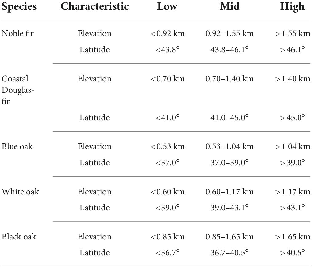
Table 2. Description of the nine naïve-divisions of habitat for each species based on the cross-combination of three partitions (Low, Mid, High) of the elevational and latitudinal range of each species (Characteristic).

Observed mortality and net-growth

We estimated the observed net-growth and mortality that occurred over a recent 10-year period within the species’ estimated range, naïve-divisions, and (for each MCMC sample) PECA-divisions. These observed data come from FIA-plots first measured (t1) between 2001–2011 and remeasured (t2) ^~10 years later between 2011 and 2019. Data were downloaded and queried from the FIA databases for OR, WA, and CA on May 12, 2022 [for documentation and access information, see Burrill et al. (2021)].

Definitions of growth and mortality

We report net-growth and mortality in units of annualized trees per ha (TPH/year) and basal-area per ha [cross-sectional area (cm²) at 1.37 m per ha per year; BAH/year] on forest land where the species was present (at t1 for mortality and at either t1 or t2 for net-growth). The FIA program only recorded species data in areas (called “conditions” by the FIA Program) qualifying as forest land within FIA-plots, which is currently defined as conditions with greater than 10% tree canopy cover. Therefore, estimates of net-growth and mortality will reflect this forest land definition. However, to focus on climate impacts and avoid estimates that account for reversion or diversion (i.e., the movement of land into or out of the forest-land base), we only estimated mortality and net-growth on conditions classified as forest land at both t1 and t2. Because not all plots are measured exactly 10 years after the t1 measurement, we annualized estimates to account for slight variability in plots’ remeasurement-periods. We consider tally-trees (diameter ≥ 12.7 cm at 1.37 m) in our definition, because they are more reliably tracked by the FIA program than smaller diameter trees, which only began to be tagged in the PNW in 2010 (USDA Forest Service, 2010). However, the SDMs we used for prediction were fit with presence-absence data for trees with diameters ≥ 2.54 cm (Kralicek, 2022a). Therefore, the trees used to fit the SDMs may or may not have met the diameter-threshold for a tally-tree by their plot’s remeasurement date. With respect to observed change estimates, we hereafter refer to tally-trees as trees.

We define net-growth and mortality as in Scott et al. (2005). Because our aim was to examine potential climate change impacts, we focus on trees that died of natural causes (mortality) and distinguish this from trees killed due to human activity (removals), such as harvests or silvicultural operations which may or may not lead to the tree’s physical removal from the plot. Therefore, mortality is the units (i.e., BAH/year or TPH/year) of trees that have died of natural causes between t1 and t2. Net-growth is the change in units of trees that occurred between t1 and t2 and is defined as the difference between gross growth and mortality. As in Scott et al. (2005), we assume that death for both mortality and removal trees occurred at the midpoint of the remeasurement period and use a modeled midpoint-diameter in basal-area calculations (Burrill et al., 2021). Similarly, we consider as ingrowth any tree that grew past the 12.7 cm diameter-threshold prior to the midpoint of the remeasurement period. In other words, net-growth accounts for growth gains and mortality, while not deducting losses from removals or land-use change.

Where climate change impacts are particularly advanced, we expect declines in basal area (i.e., negative net-growth BAH/year) accompanied by ingrowth that does not exceed trees lost due to mortality (i.e., negative net-growth TPH/year). Therefore, to assess the sustainability of mortality, we defined unsustainable mortality as mortality that exceeded growth (i.e., negative net-growth) both in terms of TPH/year and BAH/year. We also examined the relative amounts of growth and mortality by estimating net-growth as a percentage of gross growth (growth prior to deductions from mortality losses), which we hereafter refer to as relative-growth. While relative-growth relays similar information to net-growth, it allows a more direct comparison between mortality and growth. For example, if TPH/year-based relative-growth is -100%, then the number of mortality trees was twice that of ingrowth. Similarly, BAH/year-based relative-growth of 50 or 100% indicates that net-growth was half of or equal to gross growth, respectively. However, it should be noted that this statistic can only be calculated for non-zero values of gross growth and large percentages will be estimated when the magnitude of net-growth is much larger than that of gross growth. Nevertheless, such statistics have been used to assess the stability of populations (Goeking and Windmuller-Campione, 2021).

Estimation

The FIA Program implements a quasi-systematic sampling design and uses post-stratification to increase precision and reduce bias from non-response and varying sampling intensity across ownerships (e.g., to account for higher plot density on non-wilderness than wilderness National Forest System lands in OR and WA). We calculated means and variances based on the post-strata defined by the FIA Program and using the (design-based) post-stratified estimators in Scott et al. (2005; Equations 4.16 and 4.17 for stratified estimation with known strata weights). We then calculated equal-tailed, 90% confidence intervals for all estimates (e.g., net-growth BAH/year).

When considering estimators for the sample variance of the post-stratified mean, it is important to note that, while the computational burden of design-based estimators is less than that of model-based estimators, a design-based estimator will be conservative for a quasi-systematic sample like the FIA Program’s annual inventory (Frank and Monleon, 2021). The conservative nature of these variance estimates will result in a positive-bias and wider confidence intervals than the stated rate (i.e., a “90-percent” CI will have coverage probabilities > 0.9). When post-stratified estimation is used for (quasi-)systematic sampling designs, design-based variance estimators are either very unstable [quasi-systematic; Stevens and Olsen (2003)] or intractable [if strictly systematic; Särndal et al. (2003)]. Therefore, design-based estimators like those in Scott et al. (2005) assume simple random sampling within strata and proportional allocation of plots between strata. Recent research has demonstrated that model-based variance estimators can reduce the positive-bias incurred by the simple random sampling assumption of design-based estimators (Frank and Monleon, 2021). However, in this study, we apply the design-based variance estimators of Scott et al. (2005) and note that the resulting variance estimates will be conservative.

Although uncommon across species, we encountered machine precision issues when calculating the estimate or standard error of the mean for one or more statistics due to the denominator of the estimator (e.g., total area within the domain-of-interest, such as ha of forest land where the species was present at t1) being close to zero. Across all species, this happened for mortality and net-growth statistics in 1–10% of the MCMC samples’ PECA-divisions (across all species), depending on the future climate scenario. Machine precision issues were more common when calculating relative-growth statistics (14–24%) and were the most common when calculating relative-growth TPH/year for blue oak (48–71%).

Comparisons between PECA-divisions

To determine if observational data indicated that species were already experiencing projected impacts of climate change, we assessed the sustainability of mortality within PECA-divisions and compared estimates of net-growth and mortality between PECA-divisions. While the 90% confidence intervals for estimates represent the variance in field measurements of, e.g., net-growth, the MCMC sampling represents the uncertainty in the species’ geographical range estimates. Therefore, we accounted for both sources of uncertainty by examining trends in net-growth, mortality, and relative-growth within the PECA-divisions across all 100 MCMC samples.

First, we assessed the sustainability of mortality within PECA-divisions and quantified how often MCMC samples agreed on the direction of observed change. For each MCMC sample and PECA-division, we classified the type of net-growth and mortality for both TPH/year- and BAH/year-based statistics. Classifications were based on 90% confidence intervals for estimates and were classified as “zero” if zero was within the interval, “positive” if the interval’s lower-bound was greater than zero, or “negative” if the interval’s upper-bound was less than zero. To quantify the uncertainty in these classifications across estimates of species’ geographic ranges, we report for each PECA-division the percent of MCMC samples classified as each of these three classes and how often mortality was unsustainable (i.e., negative net-growth BAH/year and TPH/year within the same MCMC sample).

For species already experiencing climate change impacts, we expect that areas of contraction (i.e., where habitat is projected to become unsuitable) will have higher mortality and lower net-growth than areas of expansion (become suitable). Where impacts are particularly advanced, we expect that areas of contraction will also have higher mortality and lower net-growth than areas of persistence (remain suitable), with the same being true for areas of persistence when compared with areas of expansion. To tests these hypotheses, we performed one-sided z-tests (0.1-level; Casella and Berger, 2002) to compare estimates between these PECA-divisions. Specifically, for each MCMC sample and type of statistic (i.e., BAH/year or TPH/year), we tested that mortality was significantly higher (test 1) and that net-growth was significantly lower (test 2) in areas of (1) contraction than persistence, (2) contraction than expansion, and (3) persistence than expansion. The corresponding null hypotheses for, e.g., test 1 was that mortality in contraction areas was not significantly higher than mortality in persistence areas. Tests could only be performed for MCMC samples for which, e.g., mortality could be estimated in both contraction and persistence PECA-divisions. From the set of MCMC samples for which both z-tests could be performed, we quantified the uncertainty due to species’ geographical range estimates by reporting the percent of MCMC samples for which: (1) mortality was not (significantly) higher and net-growth was not lower; (2) mortality was higher, but net-growth was not lower; (3) net-growth was lower, but mortality was not higher, or (4) mortality was higher and net-growth was lower. It is important to note that, through the variance estimates used in these z-tests, uncertainty information from the FIA sampling design is incorporated into these percent-agreement summaries. Therefore, due to our use of a design-based variance estimator, these tests will also be conservative.

Results

In this section, we begin by reporting a high-level overview of the projected climate-change impacts for each species under the four future climate scenarios. We then report observed change (e.g., net-growth) for each species across all forest land on which the species was present and for naïve, one-third divisions of habitat based on elevation and latitude. We then present and compare estimates of observed change within divisions of habitat based on where habitat is projected to expand, persist, or contract by the 2080s under the four future climate scenarios (i.e., PECA-divisions).

Projected impacts of climate change

For all species, projected climate-change impacts closely mirror results from the study for which the species-specific SDMs were originally developed (Kralicek, 2022a), which provides an in-depth discussion of these impacts. Here, we review those projected impacts in brief as they relate to our analysis of mortality and net-growth.

For coastal Douglas-fir, the maps in Figure 1 show the most commonly assigned PECA-divisions for each FIA-plot in the species’ study area (i.e., the mode across the 100 MCMC samples) as well as the assignment of the elevation- and latitude-based naïve-divisions of habitat. Similar Figures are provided in Supplementary appendix B for noble fir (Supplementary Figure B.1), blue oak (Supplementary Figure B.2), white oak (Supplementary Figure B.3) and black oak (Supplementary Figure B.4). The location of climatically suitable habitat for species generally shifted upwards in elevation or northward in latitude from the current mean-predictions as lower elevation or more southernly latitudes became less suitable (e.g., Figure 1). Climate change impacts generally became more pronounced with increasing severity of the future climate scenario; that is, from the mildest scenario under an intermediate emissions pathway and median climate projection (RCP 4.5 CCSM4) to the most severe scenario under a high emissions pathway and worst-case climate projection (RCP 8.5 HadGEM2-ES). While mean-predictions for noble fir generally decreased regardless of elevation or latitude (Supplementary Figure B.1), elevation had a stronger impact on changes to climatically suitable habitat for black oak than latitude (Supplementary Figure B.4). Both elevation and latitudinal shifts in habitat were evident in the mean-predictions for coastal Douglas-fir (Figure 1), blue oak (Supplementary Figure B.2), and white oak (Supplementary Figure B.3).

FIGURE 1

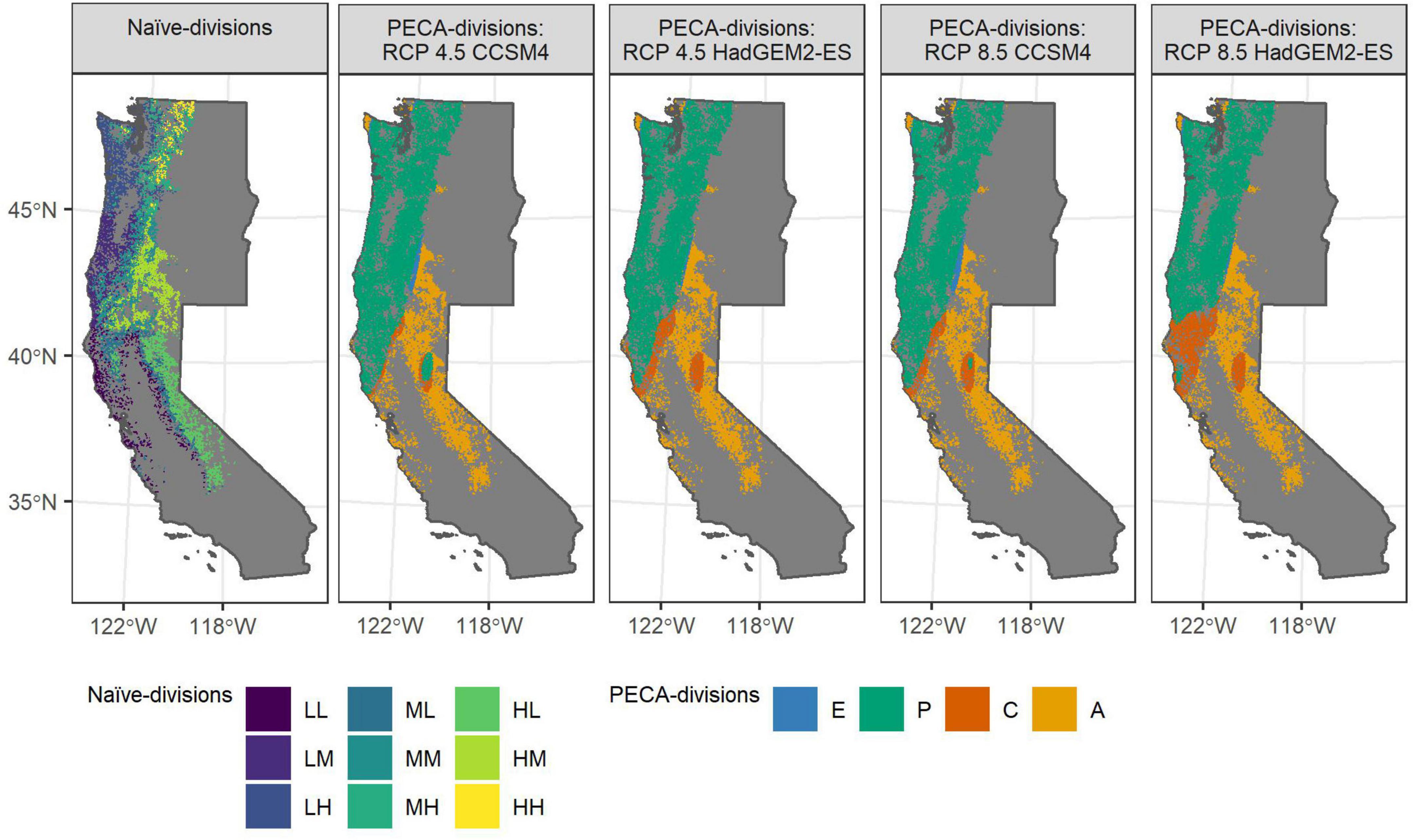
Figure 1. For coastal Douglas-fir, maps of FIA plots within the species’ study area where plots are colored by the naïve-division and by the most commonly assigned PECA-division (across the 100 MCMC samples) under each of the four future climate scenarios. Future climate scenarios are organized from left to right by increasing severity, from the mildest scenario (RCP 4.5 CCSM4) to the most severe (RCP 8.5 HadGEM2-ES). The first and second letters of the naive-divisions code (Table 2) corresponds to the elevation-partition and the latitude-partition, respectively; e.g., ML is the mid-elevation, low-latitude naïve-division. PECA-divisions correspond to areas of projected range expansion (E), persistence (P), contraction (C), or where habitat for the species was projected to remain unsuitable (A).

Relative to the current estimate of range-size, the species with the greatest change in range-size were noble fir and forest-land white oak. By the 2080s, total habitat was projected to shrink by between 79–100% for noble fir and between 9–49% for white oak under the four future climate scenarios (Table 3). For noble fir, there was no significant area of persistence or expansion for all but the mildest scenario (RCP 4.5 CCSM4) under which 21% of noble fir’s current range was projected to remain climatically suitable (Table 3); less than 12 km² of range persistence or expansion (posterior mean) was projected under all other scenarios. For white oak, 21–59% of its current range was projected to become unsuitable and only 10–14% was projected to be replaced by expansion area (Table 3).

TABLE 3

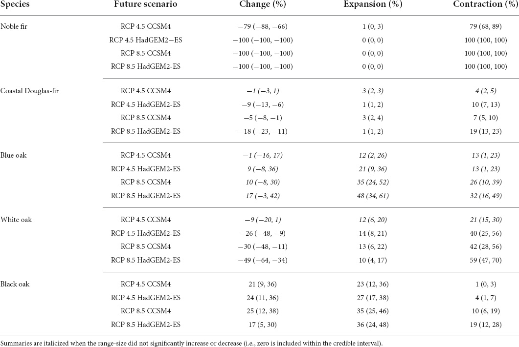
Table 3. Posterior means and equal-tailed 90% credible intervals for the relative-change (Change; %) in range-size estimates and the relative area of expansion and contraction (%; area relative to the current range-size estimate) by species under the four future climate scenarios.

Net-losses in habitat were also projected for coastal Douglas-fir under most future climate scenarios, although 81–96% of its current range was projected to remain suitable (Table 3). While no significant change in range-size was projected for blue oak, 21–59% of the current range was projected to become unsuitable (Table 3). Black oak was the only species for which overall net-gains in habitat were projected (Table 3). Nevertheless, 10–19% of black oak’s currently suitable habitat was projected to become unsuitable by the 2080s under the RCP 8.5 scenarios (Table 3).

Observed change within overall range and naïve-divisions of habitat

For each species, the observed net-growth, mortality, and relative-growth over a recent 10-year period is presented in Table 4 in terms of BAH/year and TPH/year on forest land where the species was present. When estimated across the species’ current distribution, all species except black oak were increasing or stable at this meta-population level (Table 4). Net-growth TPH/year and BAH/year were positive for noble fir, coastal Douglas-fir, and white oak. Blue oak also had positive net-growth BAH/year, although ingrowth was balanced by mortality trees (i.e., net-growth TPH/year not significantly different from zero). Black oak was the only species with significantly negative net-growth, both in terms of TPH/year and BAH/year, with the number of mortality trees more than twice that of ingrowth (relative-growth TPH/year, Table 4). Among the species, relative-growth was highest for coastal Douglas-fir, for which net-growth was more than half the value of growth before losses due to mortality were deducted (59 and 75%, when calculated based on TPH/year- and BAH/year-based statistics, respectively).

TABLE 4

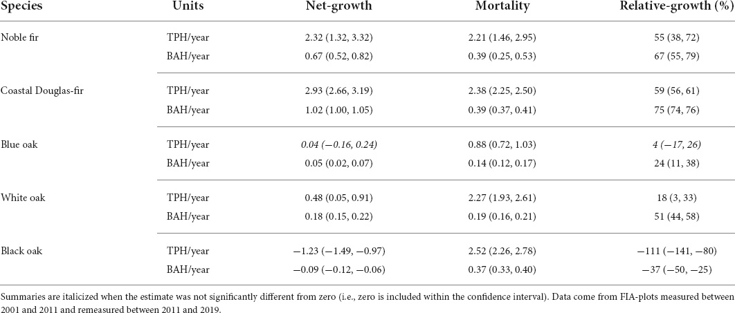
Table 4. Estimate and equal-tailed 90% confidence intervals for net-growth, mortality, and relative-growth (i.e., net-growth expressed as a percentage of gross growth, which is net-growth plus mortality) for the five species in terms of the BAH/year and TPH/year (units) on forest land where the species was present.

The prevalence of each species at t1 (first plot measurement) within its species-specific naïve-divisions of habitat is presented in Figure 2. Prevalence was less than one percent in at least one naïve-division for noble fir (LL, HM, HH), blue oak (MH, HM, HH), white oak (HL, HH), and black oak (LL, HH). We were unable to estimate, e.g., net-growth for species that did not occur within a given naïve-division (colored red in Figure 2). The observed net-growth of each species within naïve-divisions is presented in Figure 3; similar figures for mortality and relative-growth are provided in Supplementary Figures C.1, C.2, respectively.

FIGURE 2

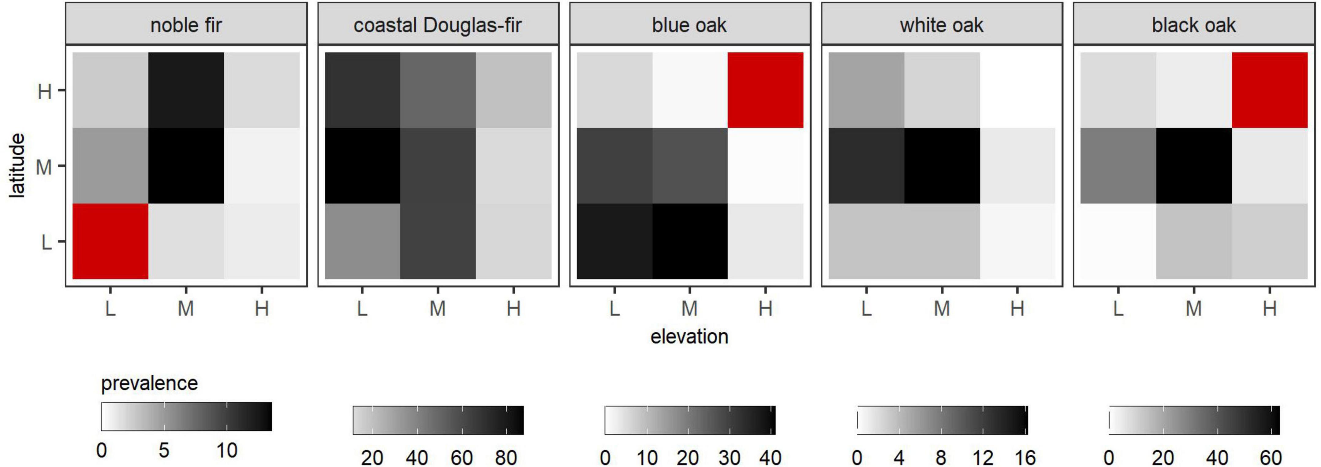
Figure 2. The percent of plots on which species were present at the first plot measurement (prevalence) within naïve-divisions of habitat based on elevation and latitude. Darker shading corresponds to higher species prevalence and cells colored red correspond to naïve-divisions within which the species was not present on forest land. Naïve-divisions are shown according to their elevation- and latitude-partitions, e.g., low (L), mid (M), or high (H) elevation or latitude. The first and second letters of the naive-divisions code (Table 2) correspond to these elevation- and latitude-partitions (e.g., LM for low-elevation and mid-latitude); see Table 2 for individual naïve-division definitions.

FIGURE 3

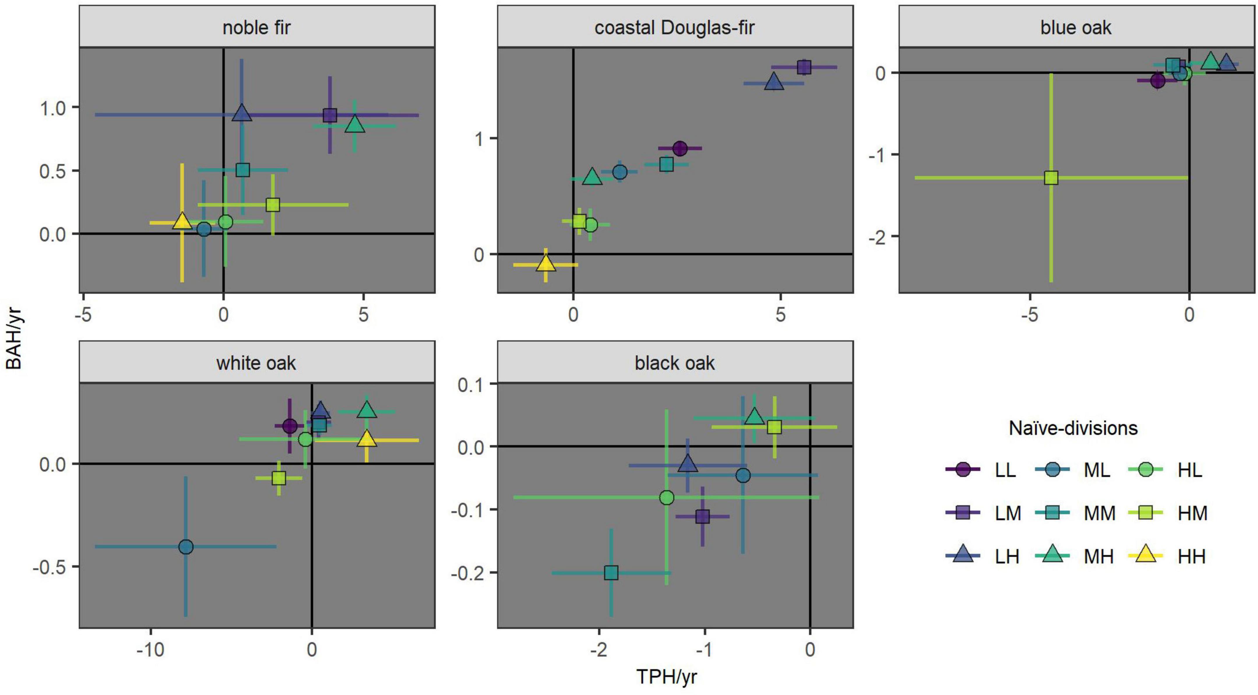
Figure 3. Estimates and equal-tailed 90% confidence intervals for net-growth within naïve-divisions of habitat (based on elevation and latitude; naïve-divisions) in terms of the BAH/year and TPH/year on forest land where the species was present. The first and second letters of the naive-divisions code (Table 2) correspond to the elevation- and latitude-partitions, respectively (e.g., LM for low-elevation and mid-latitude); see Table 2 for individual naïve-division definitions. A value of zero net-growth BAH/year or TPH/year is indicated by the black lines for reference.

Across species, mortality was sustainable with increasing or stable meta-populations for most naïve-divisions of habitat (i.e., net-growth BAH/year not significantly negative; Figure 3). However, only noble-fir and coastal Douglas-fir had sustainable mortality for all naïve-divisions for which estimates were possible (Figures 2, 3). Noble fir was increasing (i.e., net-growth BAH/year and TPH/year both significantly positive) at the low elevation and mid latitude (LM) and at the mid elevation and high latitude (MH) naïve-divisions. At high elevation and high latitude (HH) naïve-division where noble fir prevalence was low, ingrowth did not offset mortality in terms of TPH/year although net-growth BAH/year of noble fir was stable (Figure 3). Coastal Douglas-fir was increasing at the low-elevation naïve-divisions (i.e., LL, LM, LH) and at the mid elevation and low-to-mid latitudes naïve-divisions (ML, MM; Figure 2).

All oak species had decreasing meta-populations within at least one naïve division (i.e., net-growth BAH/year and TPH/year both significantly negative; Figure 3). Forest-land blue oak was decreasing within the high elevation and mid latitude (HM) naïve-division (Figure 3), a naïve-division in which prevalence of this species on forest land was less than one percent (Figure 2). Otherwise, blue oak was increasing within the low elevation and high latitude (LH) naïve-division and stable elsewhere. Apart from HM naïve-division, ingrowth from forest-land blue oak only failed to offset the number of mortality trees within the low elevation and low latitude (LL) naïve-division.

Forest-land white oak was decreasing within the mid elevation and low latitude (ML) naïve-division, increasing within the mid-to-high elevation and high latitude (MH, HH) naïve-divisions, and otherwise stable (Figure 3). The number of mortality trees of forest-land white oak exceeded ingrowth within the low-to-mid elevation and low latitude (LL, ML) and high elevation and mid latitude (HM) naïve divisions.

Black oak was decreasing within the low-to-mid elevation and mid latitude (LM, MM) naïve divisions, but otherwise stable (Figure 3). Ingrowth did not offset black oak mortality TPH/year within the mid elevation and mid latitude (MM) naïve-division and all the low elevation naïve-divisions except for LL where black oak prevalence was less than one percent (i.e., LM and LH; Figure 3).

Comparing projected impacts to observed change

For each species, estimates and 90% confidence intervals for net-growth BAH/year and TPH/year in areas projected to become climatically suitable (expand), remain climatically suitable (persist), become climatically unsuitable (contract), or remain climatically unsuitable (remain absent) under the four future climate scenarios were estimated for each of the 100 MCMC samples (Supplementary Figure C.3). For some species and MCMC samples, it was impossible to estimate mortality or net-growth for PECA-divisions, because a PECA-division was either too small in area or had too few field-plots on which the species was present to make estimates for specific statistics. This was a common case for noble fir because most scenarios resulted in high contraction with little expansion; only six of the 100 MCMC samples were able to produce mortality or net-growth estimates within an estimated area of expansion under the mildest scenario (RCP 4.5 CCSM4), and only one MCMC sample under any of the three more severe future scenarios was able to produce an estimate within an estimated area of persistence (RCP 8.5 CCSM4).

For each species and PECA-division under the mildest future scenario (RCP 4.5 CCSM4), Figure 4 shows the percent of MCMC samples for which net-growth and mortality were classified as being significantly positive, negative, or not different from zero (based on equal-tailed, 90% confidence intervals for these estimates) in terms of BAH/year and TPH/year. Similar figures to Figure 4 are provided in Supplementary appendix C for RCP 4.5 HadGEM2-ES (Supplementary Figure C.4), RCP 8.5 CCSM4 (Supplementary Figure C.5), and RCP 8.5 HadGEM2-ES (Supplementary Figure C.6). In general, summaries for net-growth TPH/year statistics tended to be positive less often than BAH/year statistics across species. Because substantial range contraction was projected for noble fir (Table 3), the summaries for contraction predominantly represent estimates for the entirety of this species’ current range, especially for the three more severe future climate scenarios where 100% range contraction was projected by the majority of MCMC samples. Therefore, results in Figure 4 and Supplementary Figures C.4–C.6 mimic those in Table 4 for noble fir with growth that exceeded mortality in terms of BAH/year and TPH/year (i.e., positive net-growth).

FIGURE 4

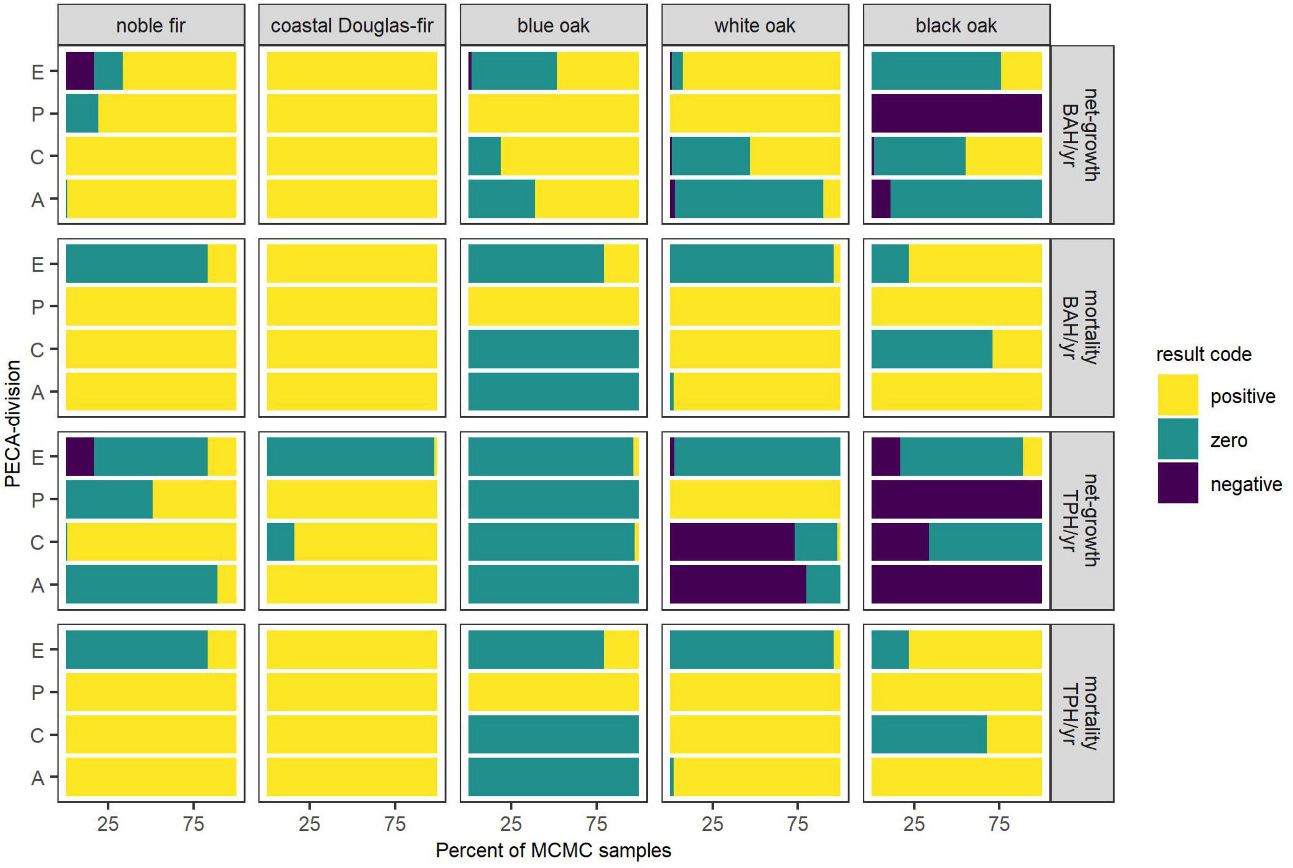
Figure 4. For each species and PECA-division under the RCP 4.5 CCSM4 (mildest) scenario, the percent of MCMC samples for which equal-tailed 90% confidence intervals for estimates of net-growth and mortality, in terms of BAH/year or TPH/year, were classified as positive (lower bound of interval greater than zero), zero (zero within interval), or negative (upper bound of interval less than zero). Per-ha estimates are for forest land where the species was present within the PECA-divisions, that is, areas of projected expansion (E), persistence (P), contraction (C), and where habitat was projected to remain climatically unsuitable (A). Percentages are based on MCMC samples for which an estimate was possible.

Nearly 100% of MCMC samples for coastal Douglas-fir and white oak on forest land (i.e., land where canopy cover of trees exceeded 10%) had growth BAH/year exceeding mortality across PECA-divisions and future climate scenarios, suggesting mortality was sustainable, including in areas of projected contraction (Figure 4 and Supplementary Figures C.4–C.6). In terms of TPH/year, only areas of expansion for coastal Douglas-fir commonly had growth equivalent to mortality, while all other areas had positive net-growth for this species. For white oak, the number of mortality trees was equivalent to ingrowth in areas of expansion, less than ingrowth in areas of persistence, and equivalent to or greater than ingrowth in areas of contraction; these patterns for coastal Douglas-fir and white oak generally held across future climate scenarios.

Across most future climate scenarios for blue oak on forest land, growth exceeded or was equivalent to mortality across PECA-divisions, both in terms of TPH/year and BAH/year, suggesting sustainable mortality when estimates were made at the level of these PECA-divisions. While most MCMC samples resulted in growth estimates equivalent to mortality, in areas of persistence and contraction net-growth BAH/year was more often significantly positive. The only exception was in areas of contraction under the most severe climate scenario (RCP 8.5 HadGEM2-ES) where mortality was still sustainable, but the majority of MCMC samples resulted in the number of mortality trees exceeding ingrowth and growth BAH/year more often equivalent to mortality BAH/year (Supplementary Figure C.6).

Although greater than 80% of black oak’s current range was projected to remain climatically suitable under the four future climate scenarios, mortality exceeded growth in areas projected to persist under all scenarios (Figure 4 and Supplementary Figures C.4–C.6), as well as in areas projected to contract under the RCP 8.5 scenarios (Supplementary Figures C.5, C.6). Net-growth in these areas was negative both in terms of TPH/year as well as BAH/year, suggesting unsustainable mortality when estimates were made at the level of these PECA-divisions. Conversely, areas of projected expansion often had positive net-growth in terms of TPH/year and BAH/year under the RCP 8.5 scenarios, suggesting mortality was sustainable within these areas.

Estimates of mortality and net-growth are directly compared in Figure 5 between areas of contraction and persistence (Figure 5A), contraction and expansion (Figure 5B), and persistence and expansion (Figure 5C) by species and future climate scenario. Illustrated in Figure 5 is the percent of MCMC samples for which estimates of mortality were higher and/or estimates of net-growth were lower between these PECA-divisions. For noble fir, comparisons involving areas of persistence or expansion were not possible under some of the scenarios. For example, under the three more severe climate scenarios, estimates within persistence areas were only possible for one MCMC sample under one scenario (RCP 8.5 CCSM4; Figure 5A); for this one MCMC sample, the areas projected to contract had significantly higher mortality and lower net-growth than in areas where habitat was projected to remain climatically suitable (Figure 5A). Under the mildest scenario (RCP 4.5 CCSM4), far more MCMC samples allowed for comparisons between persistence and contraction for noble fir (100 MCMC samples). Areas of contraction did not tend to have significantly higher mortality or lower net-growth than areas of persistence (both in terms of BAH/year and TPH/year; Figure 5A). However, contraction and persistence areas had higher mortality than expansion areas in five out of the six MCMC samples for which expansion estimates were possible under the RCP 4.5 CCSM4 scenario (Figures 5B,C).

FIGURE 5

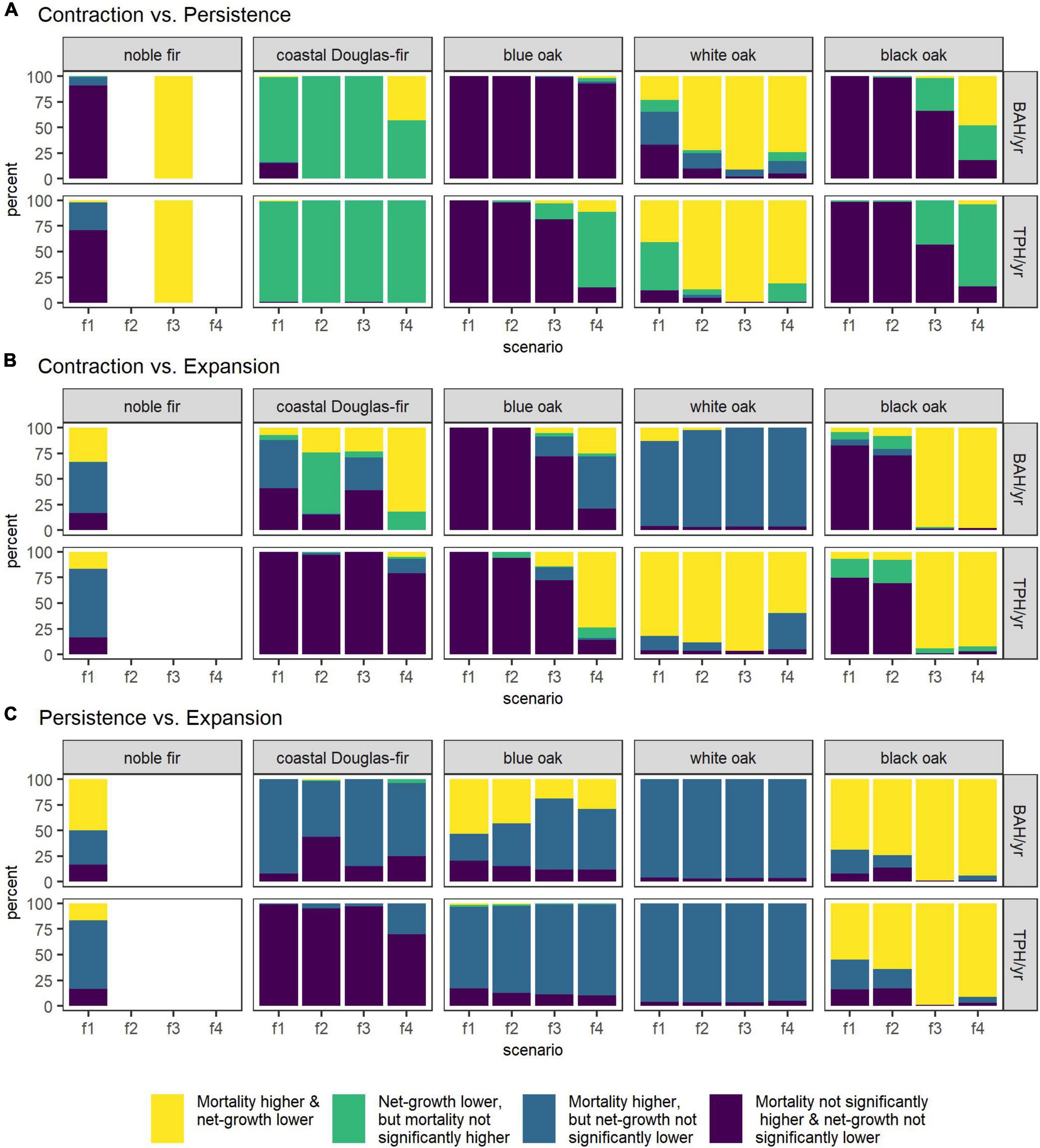
Figure 5. The percent-agreement between PECA-divisions’ estimates across MCMC samples by species (column) and future climate scenario (x-axis) based on two one-tailed z-tests (0.1-level): one for higher mortality and one for lower net-growth in areas of contraction than persistence (A), contraction than expansion (B), and persistence than expansion (C). Results are shown for BAH/year and TPH/year estimates of mortality and net-growth on forest land where the species was present. Future climate scenarios are coded by increasing severity as: RCP 4.5 CCSM4 (f1; mildest scenario), RCP 4.5 HadGEM2-ES (f2), RCP 8.5 CCSM4 (f3), and RCP 8.5 HadGEM2-ES (f4).

For coastal Douglas-fir, areas of contraction consistently had lower net-growth than areas of persistence both in terms of BAH/year and TPH/year, although mortality was only significantly higher in areas of contraction under the most severe scenario (RCP 8.5 HadGEM2-ES, in 43% of MCMC samples; Figure 5A). Across future scenarios, areas of persistence tended to have higher mortality BAH/year than areas of expansion (Figure 5C). However, in terms of TPH/year, areas of persistence or contraction did not have significantly higher mortality nor significantly lower net-growth than expansion areas (Figures 5B,C). When comparing areas of contraction and expansion (Figure 5B), CCSM4 future scenarios (i.e., a median-projection climate model) resulted in contraction areas with higher mortality BAH/year, but not significantly lower net-growth than expansion areas. The HadGEM2-ES future scenarios (i.e., a worst-case-projection climate model) resulted in contraction areas with significantly lower net-growth BAH/year, but only the most severe climate scenario also resulted in significantly higher mortality BAH/year (RCP 8.5 HadGEM2-ES; Figure 5B).

Mortality of forest-land blue oak was higher in areas projected to persist than in expansion areas, both in BAH/year and TPH/year for most MCMC samples under all future scenarios (Figure 5C). Areas of persistence also often had lower net-growth BAH/year than expansion areas under the RCP 4.5 scenarios (Figure 5C). For most scenarios, areas of contraction did not have significantly higher mortality nor significantly lower net-growth than areas of persistence or expansion across most MCMC samples. The exception to this was under most severe future scenario (RCP 8.5 HadGEM2-ES), for which areas of contraction had lower net-growth TPH/year than areas of persistence and expansion, and higher mortality, both in terms of BAH/year and TPH/year, than areas of expansion (Figures 5A,B).

Contraction areas had higher mortality and lower net-growth of forest-land white oak than areas of persistence (BAH/year and TPH/year) and expansion (TPH/year) for the majority of MCMC samples under most future scenarios (Figures 5A,B). Compared with areas of expansion, mortality was higher in areas of contraction (BAH/year; Figure 5B) and persistence (BAH/year and TPH/year; Figure 5C).

Under all scenarios for black oak, areas of persistence had higher mortality and lower net-growth than areas of expansion, both in terms of BAH/year and TPH/year, for the majority of MCMC samples (Figure 5C). Under the RCP 4.5 scenarios, areas of contraction did not tend to have significantly higher mortality nor lower net-growth than areas of persistence or expansion (Figures 5A,B). While both areas of contraction and persistence under the RCP 8.5 scenarios had negative net-growth for the majority of MCMC samples (Supplementary Figures C.4, C.5), under the most severe scenarios (RCP 8.5 HadGEM2-ES) areas of contraction had lower net-growth (BAH/year and TPH/year) and higher mortality (BAH/year) than areas of persistence (Figure 5A). When compared with areas of expansion, both RCP 8.5 scenarios had higher mortality and lower net-growth in areas of contraction than expansion (BAH/year and TPH/year; Figure 5B).

Discussion

We found that observed changes in net-growth and mortality varied by species and in some cases clearly correspond with projected changes in climatically suitable habitat for the 2080s. The manifestation of projected shifts in habitat suitability will likely vary by species, as will individual species’ responses to shifts in climatic suitability. Observed demographic rates of growth and mortality suggested that mortality was sustainable at the range-wide level for all species except black oak, where the sustainability of mortality varied by areas of projected expansion, persistence, and contraction as well as naïve-divisions of habitat based on elevation and latitude. The congruity between projections and observed change was not universal and helped highlight potential limitations in projections. In some areas, where habitat was projected to shift in suitability, indications of unsustainable mortality suggest potential species declines that merit further investigation. The MCMC methods associated with our spatial-Bayesian hierarchical models allowed us to not only quantify the variability of observed change estimates within areas where the climatic suitability of habitat was projected to shift, but to also quantify the uncertainty associated with the species’ geographical ranges estimates on which those projections were based.

Of the five species we examined, noble fir was projected to experience the most damaging impacts of climate change, with total contraction of the species’ range by the 2080s projected under three of the four future climate scenarios we examined. This finding is supported by other studies that have identified noble fir as highly vulnerable to climate change (McKenney et al., 2007; Crookston et al., 2010; Devine et al., 2012; Case and Lawler, 2016). When estimated across all forest land that noble fir currently occupies and within naïve-divisions of habitat, mortality appears sustainable with growth that exceeds or is equivalent to mortality (BAH/year and TPH/year; Table 4 and Figure 3). Nevertheless, under the mildest climate scenario (RCP 4.5 CCSM4) areas of contraction and persistence had higher mortality than areas of expansion, with some MCMC samples also having lower net-growth (BAH/year and TPH/year; Figures 5B,C). However, the case of noble fir highlights a limitation in evaluating observed change based on projected impacts: because projected impacts were so severe for noble fir, comparisons of mortality and net-growth between PECA-divisions were limited as there was very littler area of projected persistence or expansion under any of the future climate scenarios. Therefore, examining observed change at finer spatial resolutions for noble fir will likely aid in identifying areas of species decline.

Within our study area, mortality of coastal Douglas-fir appeared currently sustainable when examined across forest land, naïve-divisions of habitat, and within areas where habitat was projected to persist, expand, or contract. Across the species current range within the United States, net-growth was lower in areas projected to become unsuitable than where habitat was projected to persist under all future climate scenarios (BAH/year and TPH/year; Figure 5A). When compared with areas projected to become suitable, areas of persistence had higher BAH/year mortality but not significantly higher TPH/year mortality (Figure 5C); this may be expected as areas where habitat is already suitable will have more established populations containing trees with greater basal area on average. While the northern extent of coastal Douglas-fir’s range is not represented in our data set, others have similarly projected habitat loss at lower elevations and gains at higher elevations and northward into British Columbia (Gray and Hamann, 2013; Rehfeldt et al., 2014a; Mathys et al., 2017). Nevertheless, these projected shifts in the climatic suitability of habitat do not account for the maladaptation of genetic stock to shifts in climate (Rehfeldt et al., 2014b).

Based on species data collected on forest land between 2001–2010, we projected that range-size of forest-land blue oak would remain stable, but that 21–59% of the current range would become climatically unsuitable between now and the 2080s (Table 3). Areas where suitability was projected to decrease were primarily in the south of blue oak’s current range surrounding the Great Central Valley, however much of this area tended to remain within the persistence PECA-division. We found that observations of blue oak on forest land between 2001 and 2019 showed basal area growth that exceeded mortality, although the number of mortality trees offset gains from ingrowth during this period (Table 4). Similar patterns held where blue oak habitat was projected to persist, expand, or contract, although areas of expansion and contraction had basal area growth offset by mortality for many MCMC samples (Figure 4 and Supplementary Figures C.4–C.6). When estimates were made within the elevation- and latitude-based naïve-divisions, forest-land blue oak increased at low-elevation, high-latitude sites but decreased at high-elevation, mid-latitude sites (Figure 3). Blue oak is commonly found in oak savannahs where it grows at lower densities than is captured by the data used in our analysis (i.e., non-forest land, less than 10% tree canopy cover). Therefore, our findings pertain to forest-land blue oak, but cannot speak to climate change impacts or observe change in these lower density assemblages, where harsher growing conditions and less competition from other tree species may be found (McDonald, 1990). Indeed, areas where we projected habitat to lower in suitability agree with estimates by Brown et al. (2018) of 2015-dieback from the 2012 to 2015 California drought; a dieback event which occurred later than the data we used in the development of suitability projections.

Like blue oak, white oak is also found growing at lower densities in oak savannahs (Stein, 1990). Disentangling the impact of factors associated with contemporary decline of white oak [e.g., changes in land-use, fire, grazing, and conifer invasion; Hahm et al. (2018)], from the impact of climate change is complex (Pellatt et al., 2012). At the meta-population level, white oak appeared to be increasing when examined across forest land where the species was present (Table 4). However, when examined within naïve-divisions of habitat, forest-land white oak appeared to be increasing at higher latitudes and mid-to-high elevations but decreasing with unsustainable mortality at lower latitudes and high elevations (Figure 3). Mortality was sustainable in areas projected to expand, persist, and contract, although areas of contraction had more mortality trees than new additions from ingrowth under most climate scenarios (Figure 4 and Supplementary Figures C.4–C.6). Under the three more severe climate scenarios, areas of contraction had higher mortality and lower net-growth than the rest of the species’ current range where habitat was projected to remain suitable (Figure 5).

Despite projected gains in climatically suitable habitat for black oak by the 2080s, observed data suggested that mortality was currently unsustainable on forest land where black oak was present (Table 4). Though stable elsewhere, examining naïve-divisions of habitat showed that black oak was decreasing at mid-latitude and low-to-mid elevation sites (Figure 3). These two naïve-divisions that largely overlap with areas where black oak habitat was projected to persist when the species’ range was estimated with a bivariate kernel density estimator (Supplementary Figure B.4); this method of range estimation produces shapes with lower area-to-perimeter ratios than other methods [e.g., Voronoi polygons; Kralicek (2022a)], which in turn restricts the type of shapes that can be estimated for a species’ geographical range. However, areas projected to become suitable appeared to have sustainable mortality (Figure 4) and when comparing between PECA-divisions, projected persistence areas had higher mortality and lower net-growth than expansion areas (Figure 5C). The same was true for areas of contraction versus expansion under the RCP 8.5 scenarios, for which 10–19% of the current range was projected to become unsuitable (Table 3 and Figure 5B). While Lenihan et al. (2008) projected an expansion of hardwoods, including black oak, in California’s mixed evergreen forests by the 2080s, others have found recent declines specifically in large-diameter black oak from fire [ Long et al. (2018), in longer-term analysis of FIA data]. Around the 1700s AD in the Sierra Nevada, which overlaps much of black oak’s current range, there was a period of dry, cool temperatures that was predated and followed by a wetter and warmer period (Stine, 1996; Van Pelt, 2001; Lutz et al., 2010). Many of the tree species that established during this time, including mature black oak and coastal Douglas-fir, may be at higher risk of mortality if they are located toward the fringe of the species current range (Lutz et al., 2010). Large, mature black oak trees have elevated cultural and ecological importance in the Pacific Northwest (Long et al., 2016). However, in addition to impacts from climate change, other factors such as competition and pathogens like Phytophthora ramorum (responsible for sudden oak death) will likely continue to temper what sites black oak can occupy in the future (Devine et al., 2012; Long et al., 2016).

Conclusion

Recent 10-year remeasurement data from the FIA Program, allows for demographic trends in tree species, captured through metrics like net-growth and mortality, to be analyzed over large areas. When estimating demographic trends, early detection of a tree species’ response to climate change can benefit from distinguishing between areas where habitat will shift in climatic suitability for that species. In addition to examining naïve-divisions of habitat based on elevation and latitude, we identified where habitat was projected to persist, expand, or contract for five species under four future climate scenarios for the 2080s using spatial-Bayesian hierarchical models. The MCMC methods used to fit the models allowed us to quantify uncertainty in climate change impacts and comparisons of demographic trends between areas where habitat was projected to shift. These methods highlighted patterns in demographic trends that were masked when metrics such as net-growth were estimated at the broader, meta-population level.

Data availability statement

The R code used in this analysis is publicly available at https://doi.org/10.5281/zenodo.7055614. Imprecise-location (fuzzed) versions of raw FIA field data are available at https://apps.fs.usda.gov/fia/datamart/datamart.html. However, the raw data supporting the conclusions of this manuscript are based on confidential, precise-location coordinates for FIA field data, and as such cannot be uploaded to a public-facing repository. These data were internally archived within the Forest Inventory and Analysis Program’s file structure by KK, such that someone obtaining permission to access these data could replicate the analysis. For more information on access to precise-location FIA data see Burrill et al. (2021). Requests to access these datasets should be directed to https://www.fia.fs.usda.gov/about/about_us/#questions-requests.

Author contributions

KK and TB conceptualized the study and contributed to data curation. KK performed the formal analysis and wrote the original draft. All authors contributed to developing methodology, reviewed and edited manuscript drafts, and approved the submitted version.

Funding

This work was supported in part by the USDA Forest Service. This work was also prepared in part by employees of the USDA Forest Service as part of their official duties and is therefore in the public domain. However, the findings and conclusions in this publication are those of the authors and should not be construed to represent any official USDA or US Government determination or policy.

Acknowledgments

We would like to thank Andy Gray and Olaf Kuegler for their advice on querying and estimation of FIA data. An earlier version of this research was part of KK’s dissertation (Kralicek, 2022b).

Conflict of interest

The authors declare that the research was conducted in the absence of any commercial or financial relationships that could be construed as a potential conflict of interest.

The handling editor SH declared a shared affiliation with the authors at the time of the review.

Publisher’s note

All claims expressed in this article are solely those of the authors and do not necessarily represent those of their affiliated organizations, or those of the publisher, the editors and the reviewers. Any product that may be evaluated in this article, or claim that may be made by its manufacturer, is not guaranteed or endorsed by the publisher.

Supplementary material

The Supplementary Material for this article can be found online at: https://www.frontiersin.org/articles/10.3389/ffgc.2022.966953/full#supplementary-material

Footnotes

^ Available at https://sites.ualberta.ca/∼ahamann/data/climatena.html

References

Agne, M. C., Beedlow, P. A., Shaw, D. C., Woodruff, D. R., Lee, E. H., Cline, S. P., et al. (2018). Interactions of predominant insects and diseases with climate change in Douglas-fir forests of western Oregon and Washington. U.S.A. For. Ecol. Manage 409, 317–332. doi: 10.1016/j.foreco.2017.11.004

PubMed Abstract | CrossRef Full Text | Google Scholar

Araújo, M. B., and Peterson, A. T. (2012). Uses and misuses of bioclimatic envelope modeling. Ecology 93, 1527–1539. doi: 10.1890/11-1930.1